Inconsistency of Bayesian Inference for Misspecified Linear Models, and a Proposal for Repairing It

Abstract

We empirically show that Bayesian inference can be inconsistent under misspecification in simple linear regression problems, both in a model averaging/selection and in a Bayesian ridge regression setting. We use the standard linear model, which assumes homoskedasticity, whereas the data are heteroskedastic, and observe that the posterior puts its mass on ever more high-dimensional models as the sample size increases. To remedy the problem, we equip the likelihood in Bayes’ theorem with an exponent called the learning rate, and we propose the Safe Bayesian method to learn the learning rate from the data. SafeBayes tends to select small learning rates as soon the standard posterior is not ‘cumulatively concentrated’, and its results on our data are quite encouraging.

This arxiv publication is the very first, 2014, version of the paper:

P. D. Grünwald, and T. van Ommen. Inconsistency of Bayesian Inference for Misspecified Linear Models, and a Proposal for Repairing It. Bayesian Analysis, 12(4), December 2017.

In 2017, the second version was posted which is exactly the same as the original version except for this first page, and an updated bibliography.
The BA (Bayesian Analysis) 2017 version is quite different though: due to length constraints,

1. the BA version only reports on a small subset of the experiments done here, and refers extensively to the additional experimental experiments done in the present paper.

2. the BA version contains less details about the analytic calculations of the generalized posterior for regression.

3. the BA version contains no discussion of mix loss.

Otherwise, the paper has gone through many modifications and improvements. We refer to the BA version for:

1. A much more concise and better explanation of why small learning rates can vastly improve standard Bayes under misspecification, and why SafeBayes ‘works’.

2. A much more precise treatment of ‘hypercompression’, the phenomenon underlying problems with misspecification.

3. A much updated discussion section.

4. A demonstration that standard theorems for consistency of Bayesian inference under misspecification do not apply to our standard regression model.

Version 3 (2018) corrects the expression for $b_{n,\eta}$ in (14). We thank Tom Viering for spotting this error!

1 Introduction

The Problem

We empirically demonstrate the inconsistency of Bayes factor model selection, model averaging and Bayesian ridge regression under model misspecification on a simple linear regression problem with random design. We sample data $(X_{1},Y_{1}),(X_{2},Y_{2}),\ldots$ i.i.d. from a distribution $P^{*}$, where $X_{i}=(X_{i1},\ldots,X_{ip_{\max}})$ are high-dimensional vectors, and we allow $p_{\max}=\infty$. We use nested models $\mathcal{M}_{0},\mathcal{M}_{1},\ldots$ where $\mathcal{M}_{p}$ is a standard linear model, consisting of conditional distributions $P(\cdot\mid\beta,\sigma^{2})$ expressing that

$$Y_{i}=\beta_{0}+\sum_{j=1}^{p}\beta_{j}X_{ij}+\epsilon_{i}$$ (1)

is a linear function of $p\leq p_{\max}$ covariates with additive independent Gaussian noise $\epsilon_{i}\sim N(0,\sigma^{2})$. We equip each of these models with standard priors on coefficients and the variance, and also put a discrete prior on the models themselves. $\mathcal{M}:=\bigcup_{p=0..p_{\max}}\mathcal{M}_{p}$ does not contain the conditional ‘ground truth’ $P^{*}(Y|X)$ (hence the model is ‘misspecified’), but it does contain a $\tilde{P}$ that is ‘best’ in several respects: it is closest to $P^{*}$ in KL (Kullback-Leibler) divergence, it represents the true regression function (leading to the best squared error loss predictions among all $P\in\mathcal{M}$) and it has the true marginal variance (explained in Section 2.3). Yet, while $\tilde{P}\in\mathcal{M}_{0}$ and $\mathcal{M}_{0}$ receives substantial prior mass, as $n$ increases, the posterior puts most of its mass on complex $\mathcal{M}_{p}$’s with higher and higher $p$’s, and, conditional on these $\mathcal{M}_{p}$’s, at distributions which are very far from $P^{*}$ both in terms of KL divergence and in terms of $L_{2}$ risk, leading to bad predictive behavior in terms of squared error. Figure 1 and 2 illustrate a particular instantiation of our results, obtained when $X_{ij}$ are polynomial basis functions, i.e. $X_{ij}=S_{i}^{j}$ and $S_{i}\in[-1,1]$ uniformly i.i.d. We also show comparably bad predictive behavior for various versions of Bayesian ridge regression, involving just a single, high-but-finite dimensional model. In that case Bayes eventually recovers and concentrates on $\tilde{P}$, but only at a sample size that is incomparably larger than what can be expected if the model is correct.

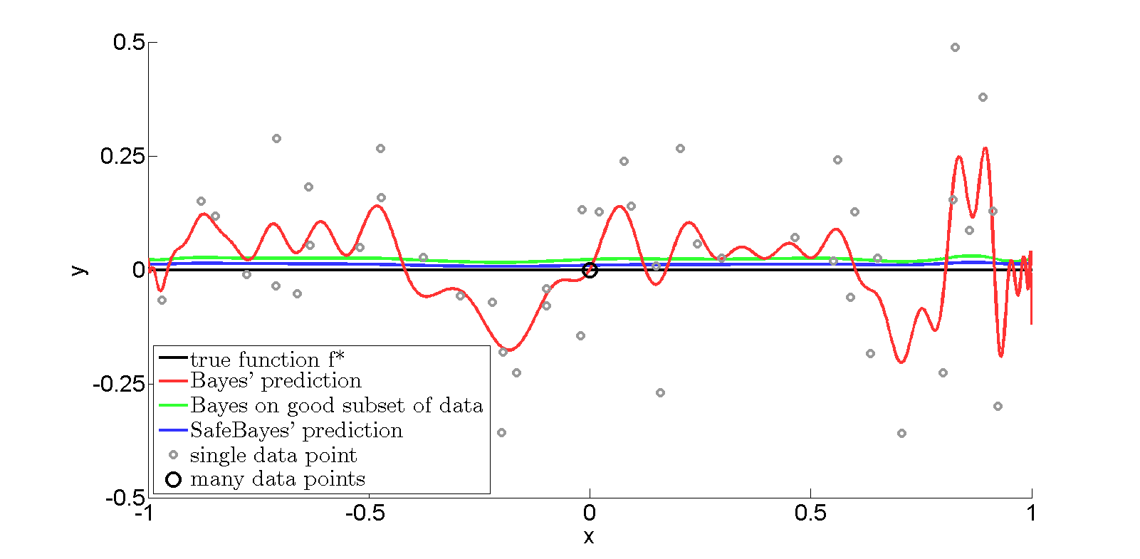
Figure 1: The conditional expectation $\mathbf{E}[Y|X]$ according to the full Bayesian posterior based on a prior on models $\mathcal{M}_{0},\ldots,\mathcal{M}_{50}$ with polynomial basis functions, given 100 data points sampled i.i.d. $\sim P^{*}$ (about 50 of which are at $(0,0)$). Standard Bayes overfits, not as dramatically as maximum likelihood/unpenalized least squares, but still enough to show dismal predictive behavior as in Figure 2. In contrast, Safe Bayes (which chooses learning rate $\eta\approx 0.4$ here) and standard Bayes trained only at the points for which the model is correct (not $(0,0)$) both perform very well.

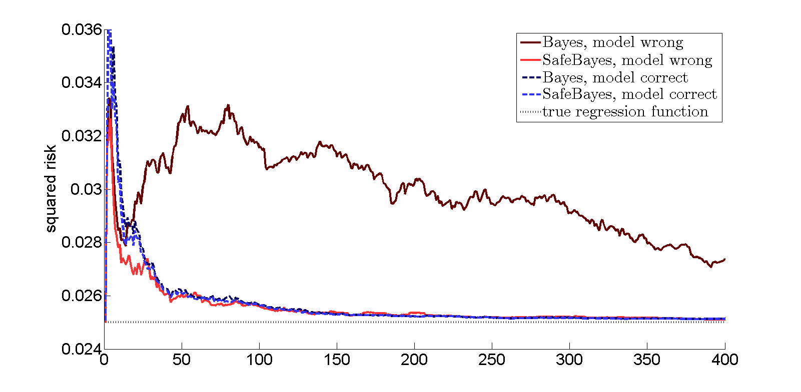
Figure 2: The expected squared error risk obtained when predicting by the full Bayesian posterior (brown curve) and the Safe Bayesian posterior (red curve) and the optimal predictions (gray curve) as a function of sample size, for the setting of Figure 1. SafeBayes is the $R$-log-version of SafeBayes defined in Section 4.2. Precise definitions and further explanation in Section 5.1 and Section 5.2.

These findings contradict the folk wisdom that, if the model is incorrect, then “Bayes tends to concentrate on neighborhoods of the distribution(s) in $\mathcal{M}$ that is/are closest to $P^{*}$ in KL divergence.” Indeed, the strongest actual theorems to this end that we know of, (Kleijn and van der Vaart, 2006, De Blasi and Walker, 2013, Ramamoorthi et al., 2015), hold, as the authors emphasize, under regularity conditions that are substantially stronger than those needed for consistency when the model is correct (as by e.g. Ghosal et al. (2000) or Zhang (2006a)), and our example shows that consistency may fail to hold even in relatively simple problems.

The Solution: Generalized Posterior and Safe Bayes

Bayesian updating can be enhanced with a learning rate $\eta$, an idea put forward independently by several authors (Vovk, 1990, McAllester, 2003, Barron and Cover, 1991, Walker and Hjort, 2002, Zhang, 2006a) and suggested as a tool for dealing with misspecification by Grünwald (2011, 2012). $\eta$ trades off the relative weight of the prior and the likelihood in determining the $\eta$-generalized posterior, where $\eta=1$ corresponds to standard Bayes and $\eta=0$ means that the posterior always remains equal to the prior. When choosing the ‘right’ $\eta$, which in our case is significantly smaller than $1$ but of course not $0$, $\eta$-generalized Bayes becomes competitive again. In general, the optimal $\eta$ depends on the underlying ground truth $P^{*}$, and the problem has always been how to determine the optimal $\eta$ empirically, from the data.

Recently, Grünwald (2012) proposed the Safe Bayesian algorithm for learning $\eta$, and theoretically showed that it achieves good convergence rates in terms of KL divergence on a variety of problems. Here we show empirically that Safe Bayes performs excellently in our regression setting, being competitive with standard Bayes if the model is correct and very significantly outperforming not just standard Bayes, but also cross-validation and approaches such as AIC when the model is incorrect. We do this by providing a wide range of experiments, varying parameters of the problem such as the priors and the true regression function and studying various performance indicators such as the squared error risk, the posterior on the variance etc.

We note that a Bayesian’s (and our) first instinct would be to learn $\eta$ itself in a Bayesian manner instead. Yet this does not solve the problem, as we show in Section 5.4, where we consider a setting in which $1/\eta$ turns out to be exactly equivalent to the $\lambda$ regularization parameter in the Bayesian Lasso and ridge regression approaches. We find that selecting $\eta$ by (empirical) Bayes, as suggested by e.g. Park and Casella (2008), does not nearly regularize enough in our misspecification experiments. In the Bayesian ridge regression setting with fixed variance, the Safe Bayesian algorithm becomes very similar to learning $\lambda$ by cross-validation with squared-error loss, as is standard in frequentist ridge regression (cross-validation with a logarithmic score does not work however). In the varying variance case, there is no such straightforward interpretation of SafeBayes.

The Type of Misspecification

The models are misspecified in that they make the standard assumption of homoskedasticity — $\sigma^{2}$ is independent of $X$ — whereas in reality, under $P^{*}$, there is heteroskedasticity, there being a region of $X$ with low and a region with (relatively) high variance. Specifically, in our simplest experiment the ‘true’ $P^{*}$ is defined as follows: at each $i$, toss a fair coin. If the coin lands heads, then sample $X_{i}$ from a uniform distribution on $[-1,1]$, and set $Y_{i}=0+\epsilon_{i}$, where $\epsilon_{i}\sim N(0,\sigma_{0}^{2})$. If the coin lands tails, then set $(X_{i},Y_{i})=(0,0)$, so that there is no variance at all. The ‘best’ conditional density $\tilde{P}$, closest to $P^{*}(Y\mid X)$ in KL divergence, representing the true regression function $Y=0$ and reliable in the sense of Section 2.3, is then given by (1) with all $\beta$’s set to $0$ and $\tilde{\sigma}^{2}=\sigma_{0}^{2}/2$. In a typical sample of length $n$, we will thus have approximately $n/2$ points with $X_{i}$ uniform and $Y_{i}$ normal with mean 0, and approximately $n/2$ points with $(X_{i},Y_{i})=(0,0)$. These points seem ‘easy’ since they lie exactly on the regression function one would hope to learn; but they really wreak severe havoc.

The In-Liers Cause the Problem

While it is well-known that in the presence of outliers, Gaussian assumptions on the noise lead to problems, both for frequentist and Bayesian procedures, in the present problem we have in-liers rather than outliers. Also, if we slightly modify the setup so that homoskedasticity holds, standard Bayes starts behaving excellently, as again depicted in Figure 1 and 2. Finally, while the figure shows what happens for polynomials, we used independent multivariate $X$’s rather than nonlinear basis functions in the main experiments below, getting essentially the same results. All this indicates that the inconsistency is really caused by misspecification, in particular the presence of in-liers, and not by anything else. The setup is inspired by the work of Grünwald and Langford (2004, 2007), who gave a mathematical proof that Bayesian inference can be inconsistent under misspecification in a related but much more artificial classification setting. Here we show that this can also happen in a much more natural regression setting. The setting being more natural, it is also harder to analyze, and we only demonstrate the inconsistency empirically.

1.1 Overview of this Paper

KL-Associated Inference tasks

Section 2 introduces our setting and the main concepts needed to understand our results. A crucial point here is that, if Bayesian (or other likelihood-based methods) converge at all to a distribution in the model $\mathcal{M}$, this distribution (often called the ‘pseudo-truth’) is the $\tilde{P}\in\mathcal{M}$ that minimizes KL-divergence to the true distribution $P^{*}$. While the minimum KL divergence point is often not of intrinsic interest, for some (not all) models, $\tilde{P}$ can be of interest for other reasons as well (Royall and Tsou, 2003): there may be associated inference tasks for which $\tilde{P}$ is suitable as well. For standard linear models with fixed $\sigma^{2}$, the main associated task is squared error prediction: the KL-optimal $\tilde{P}$ is also optimal, among all $P\in\mathcal{M}$, in terms of squared error prediction risk. If additionally $\sigma^{2}$ becomes a free parameter, then it is also reliable, which roughly means that it is optimal in determining its own squared error prediction quality (Section 2.3; we have a lot more to say about associated inference tasks in Section 7). Thus, whenever one is prepared to work with linear models and one is interested in squared risk or reliability, then Bayesian inference would seem the way to go, even if one suspects misspecification…at least if there is consistency.

The Safe Bayesian Algorithm

Section 3 introduces the $\eta$-generalized posterior and instantiates it to the linear model. Section 4 introduces the ‘Safe Bayesian’ algorithm, which learns $\eta$ from the data. This is done via Dawid’s (1984) prequential view on Bayesian inference. We then provide four instantiations of the SafeBayes method to linear models.

Section 5 discusses our experiments. We first provide the necessary preparation in Section 5.1 and 5.2. Section 5.3 gives the results of our first experiment, a comparison of Bayesian and SafeBayesian model averaging and selection in two settings, one with a correct model and one with a model corrupted by $50\%$ easy points as above, but with independent Gaussian rather than polynomial inputs. Section 5.4 repeats these experiments for a Bayesian ridge regression setting, Section 5.5 provides an ‘executive summary’. In all experiments Safe Bayesian methods behave much better in terms of squared error risk and reliability than standard Bayes if the model is incorrect, and hardly worse (sometimes still better) than standard Bayes if the model is correct.

Good vs. Bad Misspecification: Nonconcentration and Hypercompression

In and of itself, the fact that one obtains inconsistency with homoskedastic models and heteroskedastic data may not be very surprising; and indeed, whether similar phenomena occur in real-world data needs further study. The main strength of our example is rather that it clearly shows what can happen in principle, and indicates how one may go about solving it. We explain this in Section 6, in particular on the basis of Figure 9 on page 9, the essential picture to understand the phenomenon. Inconsistency can only arise under a ‘bad’ form of misspecification, depicted by the figure. Under bad misspecification, the posterior may fail to concentrate, and this causes trouble. As a theoretical contribution of this paper, we show in this section that, under some conditions, a Bayesian strongly believes that her posterior will, in some sense, concentrate fast. Indeed, SafeBayes will only select $\eta\ll 1$ if the standard posterior is nonconcentrated, and may thus be (loosely) viewed as a particular ‘prior predictive check’.

Posterior nonconcentration in turn can lead to ‘hypercompression’, the phenomenon that the Bayes predictive distribution behaves substantially better under a logarithmic scoring rule than the best distribution $\tilde{P}\in\mathcal{M}$; this can happen because the Bayes predictive distribution — a mixture of elements of $\mathcal{M}$ — behaves substantially differently from any of the elements of $\mathcal{M}$. Somewhat paradoxically (Section 6.3), Bayes’ overly good log-loss behavior is exactly what causes it to perform badly for the associated inference tasks (squared error prediction and reliability, in our case). Thus, there can be an inherent tension between behavior under log-loss and behavior under its associated tasks, a discrepancy which one can measure by the mixability gap (Section 6.4), a theoretical concept introduced by van Erven et al. (2011) and Grünwald (2012). If one is interested in log-loss, standard Bayes is just fine; the Safe Bayesian algorithm should be used if one wants to optimize behavior against the associated tasks. Of course, whether such a task-dependent modification of Bayes is desirable needs discussion, which we provide in Section 7.

Additional Experiments

The paper is followed by a long list of appendices where we provide a battery of experiments to check the robustness of our results. Specifically, we investigate what happens if we vary our models and priors (using e.g. a fixed $\sigma^{2}$ and standard priors used in the regression literature), our methods, and if we vary the data generating distribution using e.g. ‘easy’ points that are close to, but not exactly $(0,0)$. Our main conclusion here is that, of the four versions of SafeBayes which we propose, one is uncompetitive and among the other three, there is no clear winner — although they consistently outperform Bayes under misspecification. Furthermore we show that AIC, BIC and cross-validation also have serious problems in our regression setup. We also provide a proof for the theorem about nonconcentration given in Section 6.4.

2 Preliminaries: Setting, Optimal KL Distribution, Regression Function

2.1 Setting, Logarithmic Risk, Optimal Distribution

In this paper we consider data $Z^{n}=Z_{1},Z_{2},\ldots,Z_{n}\sim$ i.i.d. $P^{*}$, where each $Z_{i}=(X_{i},Y_{i})$ is an independently sampled copy of $Z=(X,Y)$, $X$ taking values in some set $\mathcal{X}$, $Y$ taking values in $\mathcal{Y}$ and $\mathcal{Z}=\mathcal{X}\times\mathcal{Y}$. We are given a model $\mathcal{M}=\{P_{\theta}\mid\theta\in\Theta\}$ parameterized by (possibly infinite-dimensional) $\Theta$, and consisting of conditional distributions $P_{\theta}(Y\mid X)$, extended to $n$ outcomes by independence. For simplicity we assume that all $P_{\theta}$ have corresponding conditional densities ${f}_{\theta}$, and similarly, the conditional distribution $P^{*}(Y\mid X)$ has a conditional ${f}^{*}$, all with respect to the same underlying measure. While we do not assume $P^{*}(Y\mid X)$ to be in (or even ‘close’ to) $\mathcal{M}$, we want to learn, from given data $Z^{n}$, a ‘best’ (in a sense to be defined below) element of $\mathcal{M}$, or at least, a distribution on elements of $\mathcal{M}$ that can be used to make predictions about future data. While our experiments focus on linear regression, the discussion in this section holds for general conditional density models. The logarithmic score, henceforth abbreviated to log-loss, is defined in the standard manner: the loss incurred when predicting $Y$ based on density ${f}(\cdot\mid x)$ and $Y$ takes on value $y$, is given by $-\log{f}(y|x)$. A central quantity in our setup is then the expected log-loss or log-risk, defined as

$$\text{\sc risk}^{\text{log}}(\theta):=\mathbf{E}_{(X,Y)\sim P^{*}}[-\log{f}_{\theta}(Y\mid X)],$$

where here as in the remainder of this paper, $\log$ denotes natural logarithm.

We let $P^{*}_{X}$ be the marginal distribution of $X$ under $P^{*}$. The Kullback-Leibler (KL) divergence $D(P^{*}\|P_{\theta})$ between $P^{*}$ and conditional distribution $P_{\theta}$ is defined as the expected KL-divergence, under $X\sim P^{*}_{X}$, of the KL divergence $D(P^{*}(\cdot\mid X)\|P_{\theta}(\cdot\mid X))$ between $P_{\theta}$ and the ‘true’ conditional $P^{*}(Y|X)$: $D(P^{*}\|P_{\theta})=E_{X\sim P^{*}_{X}}[D(P^{*}(\cdot|X)\|P_{\theta}(\cdot|X))]$. A simple calculation shows that for any $\theta$, $\theta^{\prime}$,

$$D(P^{*}\|P_{\theta})-D(P^{*}\|P_{\theta^{\prime}})=\text{\sc risk}^{\text{log}}(\theta)-\text{\sc risk}^{\text{log}}(\theta^{\prime}),$$

so that the closer $P_{\theta}$ is to $P^{*}$ in terms of KL divergence, the smaller its log-risk, and the better it is, on average, when used for predicting under the log-loss.

Now suppose that $\mathcal{M}$ contains a unique distribution that is closest, among all $P\in\mathcal{M}$ to $P^{*}$ in terms of KL-divergence. We denote such a distribution, if it exists, by $\tilde{P}$. Then $\tilde{P}=P_{\theta}$ for at least one $\theta\in\Theta$; we pick any such $\theta$ and denote it by $\tilde{\theta}$, i.e. $\tilde{P}=P_{\tilde{\theta}}$, and note that it also minimizes the log-risk:

$$\text{\sc risk}^{\text{log}}(\tilde{\theta})=\min_{\theta\in\Theta}\text{\sc risk}^{\text{log}}(\theta)=\min_{\theta\in\Theta}\mathbf{E}_{(X,Y)\sim P^{*}}[-\log{f}_{\theta}(Y\mid X)].$$ (2)

We shall call such a $\tilde{\theta}$ optimal.

Since, in regions of about equal prior density, the log Bayesian posterior density is proportional to the log likelihood ratio, we hope that, given enough data, with high $P^{*}$-probability, the posterior puts most mass on distributions that are close to $P_{\tilde{\theta}}$ in KL-divergence, i.e. that have log-risk close to optimal. Indeed, all existing consistency theorems for Bayesian inference under misspecification express concentration of the posterior around $P_{\tilde{\theta}}$.

2.2 A Special Case: The Linear Model

Fix some $p_{\max}\in\{0,1,\ldots\}\cup\{\infty\}$. We observe data $Z_{1},\ldots,Z_{n}$ where $Z_{i}=(X_{i},Y_{i})$, $Y_{i}\in{\mathbb{R}}$ and $X_{i}=(1,X_{i1},\ldots,X_{ip_{\max}})\in{\mathbb{R}}^{p_{\max}+1}$. Note that this is as in (1) but from now on we adopt the standard convention to take $X_{0i}\equiv 1$ as a dummy random variable. We denote by $\mathcal{M}_{p}=\{P_{p,\beta,\sigma^{2}}\mid(p,\beta,\sigma^{2})\in\Theta_{p}\}$ the standard linear model with parameter space $\Theta_{p}:=\{(p,\beta,\sigma^{2})\mid\beta=(\beta_{0},\ldots,\beta_{p})^{T}\in{\mathbb{R}}^{p+1},\sigma^{2}>0\}$, where the entry $p$ in $(p,\beta,\sigma^{2})$ is redundant but included for notational convenience. We let $\Theta=\bigcup_{p=0..p_{\max}}\Theta_{p}$. $\mathcal{M}_{p}$ states that for all $i$, (1) holds, where $\epsilon_{1},\epsilon_{2},\ldots\sim\text{i.i.d.~{}}N(0,\sigma^{2})$. When working with linear models $\mathcal{M}_{p}$, we are usually interested in finding parameters $\beta$ that predict well in terms of the squared error loss function (henceforth abbreviated to square-loss): the square-loss on data $(X_{i},Y_{i})$ is $(Y_{i}-\sum_{j=0}^{p}\beta_{j}X_{ij})^{2}=(Y_{i}-X_{i}\beta)^{2}$. We thus want to find the distribution minimizing the expected square-loss, i.e. squared error risk (henceforth abbreviated to ‘square-risk’) relative to the underlying $P^{*}$:

$$\text{\sc risk}^{\text{sq}}(p,\beta):=\mathbf{E}_{(X,Y)\sim P^{*}}(Y-\mathbf{E}_{p,\beta,\sigma^{2}}[Y\mid X])^{2}=\mathbf{E}_{(X,Y)\sim P^{*}}(Y-\sum_{j=0}^{p}\beta_{j}X_{j})^{2},$$ (3)

where $\mathbf{E}_{p,\beta,\sigma^{2}}[Y\mid X]$ abbreviates $\mathbf{E}_{Y\sim P_{p,\beta,\sigma^{2}}\mid X}[Y]$. Since this quantity is independent of the variance $\sigma^{2}$, $\sigma^{2}$ is not used as an argument of $\text{\sc risk}^{\text{sq}}$.

2.3 KL-Associated Prediction Tasks for the Linear Model: The KL-Optimal $\tilde{\theta}=(\tilde{\beta},\tilde{p},\tilde{\sigma}^{2})$ is square-risk optimal and reliable

Suppose that an optimal $\tilde{P}\in\mathcal{M}$ exists in the regression model. We denote by $\tilde{p}$ the smallest $p$ such that $\tilde{P}\in\mathcal{M}_{p}$, and define $\tilde{\sigma}^{2},\tilde{\beta}$ such that $\tilde{P}=P_{\tilde{p},\tilde{\beta},\tilde{\sigma}^{2}}$. A straightforward computation shows that for all $(p,\beta,\sigma^{2})\in\Theta$:

$$\text{\sc risk}^{\text{log}}((p,\beta,\sigma^{2}))=\frac{1}{2\sigma^{2}}\text{\sc risk}^{\text{sq}}((p,\beta))+\frac{1}{2}\log(2\pi\sigma^{2}),$$ (4)

so that the $(p,\beta)$ achieving minimum log-risk for each fixed $\sigma^{2}$ is equal to the $(p,\beta)$ with the minimum square-risk. In particular, $(\tilde{p},\tilde{\beta},\tilde{\sigma}^{2})$ must minimize not just log-risk, but also square-risk. Moreover, the conditional expectation $\mathbf{E}_{P^{*}}[Y\mid X]$ is known as the true regression function. It minimizes the square-risk among all conditional distributions for $Y\mid X$. Together with (4) this implies that, if there is some $(p,\beta)$ such that $\mathbf{E}[Y\mid X]=\sum_{j=0}^{p}\beta_{j}X_{j}=X\beta$, i.e. $(p,\beta)$ represents the true regression function, then $(\tilde{p},\tilde{\beta})$ also represents the true regression function. In all our examples, this will be the case: the model is misspecified only in that the true noise is heteroskedastic; but the model does invariably contain the true regression function.

Moreover, for each fixed $(p,\beta)$, the $\sigma^{2}$ minimizing $\text{\sc risk}^{\text{log}}$ is, as follows by differentiation, given by $\sigma^{2}=\text{\sc risk}^{\text{sq}}(p,\beta)$. In particular, this implies that

$$\tilde{\sigma}^{2}=\text{\sc risk}^{\text{sq}}(\tilde{p},\tilde{\beta}),$$ (5)

or in words: the KL-optimal model variance $\tilde{\sigma}^{2}$ is equal to the true expected (marginal, not conditioned on $X$) square-risk obtained if one predicts with the optimal $(\tilde{p},\tilde{\beta})$. This means that the optimal $(\tilde{p},\tilde{\beta},\tilde{\sigma}^{2})$ is reliable in the sense of Grünwald (1998, 1999): its self-assessment about its square-loss performance is correct, independently of whether $\tilde{\beta}$ is equal to the true regression function or not: $(\tilde{p},\tilde{\beta},\tilde{\sigma}^{2})$ correctly predicts how well it predicts.

Summarizing, for misspecified models, $(\tilde{p},\tilde{\beta},\tilde{\sigma}^{2})$ is optimal not just in KL/log-risk sense, but also in terms of square-risk and in terms of reliability; in our examples, it also represents the true regression function. We say that, for linear models, square-risk optimality, square-risk reliability and regression-function consistency are KL-associated prediction tasks: if (as we hope Bayes will do, but as we will see sometimes won’t) we can find the KL-optimal $\tilde{\theta}$, we automatically behave well in these associated tasks as well.

3 The Generalized Posterior

General Losses

The original generalized posterior is a notion going back at least to Vovk (1990) and has been developed mainly within the so-called (frequentist) PAC-Bayesian framework McAllester (2003), Seeger (2002), Catoni (2007), Audibert (2004), Zhang (2006b); see also Bissiri et al. (2016) and the discussion in Section 7. It is defined relative to a prior on predictors rather than probability distributions. Depending on the decision problem at hand, predictors can be e.g. classifiers, regression functions or probability densities. Formally, we are given an abstract space of predictors represented by a set $\Theta$, which obtains its meaning in terms of a loss function $\ell:\mathcal{Z}\times\Theta\rightarrow{\mathbb{R}}$, writing $\ell_{\theta}(z)$ as shorthand for $\ell(z,\theta)$. Following e.g. Zhang (2006b), for any prior $\Pi$ on $\Theta$ with density $\pi$ relative to some underlying measure $\rho$, we define the generalized Bayesian posterior with learning rate $\eta$ relative to loss function $\ell$, denoted as $\Pi\mid Z^{n},\eta$, as the distribution on $\Theta$ with density

$$\pi(\theta\mid z^{n},\eta):=\frac{e^{-\eta\sum_{i=1}^{n}\ell_{\theta}(z_{i})}\pi(\theta)}{\int e^{-\eta\sum_{i=1}^{n}\ell_{\theta}(z_{i})}\pi(\theta)\rho(d\theta)}=\frac{e^{-\eta\sum_{i=1}^{n}\ell_{\theta}(z_{i})}\pi(\theta)}{\mathbf{E}_{\theta\sim\Pi}[e^{-\eta\sum_{i=1}^{n}\ell_{\theta}(z_{i})}]}.$$ (6)

Thus, if $\theta_{1}$ fits the data better than $\theta_{2}$ by a difference of $\epsilon$ according to loss function $\ell$, then their posterior ratio is larger than their prior ratio by an amount exponential in $\epsilon$, where the larger $\eta$, the larger the influence of the data as compared to the prior.

If $z_{i}=(x_{i},y_{i})$ with $y_{i}\in{\mathbb{R}}$ and $x_{i}=(1,x_{i1},\ldots,x_{ip})$, and the goal is to predict $y_{i}$ given $x_{i}$, then we may take as our prediction model e.g. the set of linear predictors that predict $y_{i}$ by $\sum\beta_{j}x_{ij}=x_{i}\beta$, and as our loss function the squared error loss, $\ell_{\beta}(x_{i},y_{i})=(y_{i}-x_{i}\beta)^{2}$. We may then study the behavior of such a procedure in its own right, irrespective of a Bayesian misspecification interpretation; the experiments we perform in Appendix A.1 and A.1.2 can be interpreted in this manner.

Log-Loss and Likelihood

Now if the set $\Theta$ represents a model of (conditional) distributions $\mathcal{M}=\{P_{\theta}\mid\theta\in\Theta\}$, we may set, for $z_{i}=(x_{i},y_{i})$, $\ell_{\theta}(z_{i})=-\log{f}_{\theta}(y_{i}\mid x_{i})$ to be the log-loss as defined above. In this special case, the definition of $\eta$-generalized posterior specializes to the definition of ‘generalized posterior’ as known within the Bayesian literature (Walker and Hjort, 2002, Zhang, 2006a):

$$\pi(\theta\mid z^{n},\eta)=\frac{(\/{f}(y^{n}\mid x^{n},\theta)\/)^{\eta}\pi(\theta)}{\int(\/{f}(y^{n}\mid x^{n},\theta)\/)^{\eta}\pi(\theta)\rho(d\theta)}=\frac{(\/{f}(y^{n}\mid x^{n},\theta)\/)^{\eta}\pi(\theta)}{\mathbf{E}_{\theta\sim\Pi}[(\/{f}(y^{n}\mid x^{n},\theta)\/)^{\eta}]}.$$ (7)

Again, the larger $\eta$, the larger the influence of the likelihood. Obviously $\eta=1$ corresponds to standard Bayesian inference, whereas if $\eta=0$ the posterior is equal to the prior and nothing is ever learned. Our algorithm for learning $\eta$ will usually end up with values in between. It has long been known that in model selection and nonparametric settings, there is an issue with consistency proofs for full Bayes, Bayes MAP and MDL if we take the standard $\eta=1$, and indeed, this is part of the reason why the generalized posterior in the form (7) was derived in the first place: for example, Barron and Cover (1991) give general consistency theorems for 2-part MDL (closely related to Bayes MAP) and note that they hold for any $\eta<1$; but for $\eta=1$, additional assumptions must be made. Zhang (2006a) gives an explicit example in which the posterior shows anomalous behavior at $\eta=1$. A connection to misspecification was first made by Grünwald (2011) (see Section 7.1) and Grünwald (2012).

Generalized Predictive Distribution

We also define the predictive distribution based on the $\eta$-generalized posterior (7) as a generalization of the standard definition as follows: for $m\geq 0,m^{\prime}\geq m$, we set

$$\bar{{f}}(y_{i},\ldots,y_{i+m}\mid x_{i},\ldots,x_{i+m^{\prime}},z^{i-1},\eta) :=\mathbf{E}_{\theta\sim\Pi\mid z^{i-1},\eta}[{f}(y_{i},\ldots,y_{i+m}\mid x_{i},\ldots,x_{i+m^{\prime}},\theta)]$$

$$\phantom{:}=\mathbf{E}_{\theta\sim\Pi\mid z^{i-1},\eta}[{f}(y_{i},\ldots,y_{i+m}\mid x_{i},\ldots,x_{i+m},\theta)].$$ (8)

where the first equality is a definition and the second follows by our i.i.d. assumption. We always use the bar-notation $\bar{{f}}$ to indicate marginal and predictive distributions, i.e. distributions on data that are arrived at by integrating out parameters. If $\eta=1$ then $\bar{{f}}$ and $\pi$ become the standard Bayesian predictive density and posterior, and if it is clear from the context that we consider $\eta=1$, we leave out the $\eta$ in the notation.

• The generalized posterior is created by exponentiating the likelihood according to individual elements $\theta\in\Theta=\bigcup_{p}\Theta_{p}$ in the model and renormalizing, which is not the same as exponentiating marginal likelihoods and renormalizing. In particular, $\pi(p\mid z^{n},\eta)$ as given by (10) is in general not proportional to $(\/\bar{{f}}(y^{n}\mid x^{n},p)\/)^{\eta}\pi(p)$. Similarly, for generalized marginal distributions, as soon as $\eta\neq 1$, we have that in general

  $$\bar{{f}}(y_{i},y_{i+1}\mid x_{i},x_{i+1},z^{i-1},\eta)\neq\bar{{f}}(y_{i}\mid x_{i},z^{i-1},\eta)\cdot\bar{{f}}(y_{i+1}\mid x_{i+1},z^{i},\eta),$$

  unlike for the standard Bayesian marginal distribution for which equality holds (in Section 6.5 we encounter a further modification of the generalized posterior whose marginals do satisfy this product rule).

3.1 Instantiation to Linear Model Selection and Averaging

Now consider again a linear model $\mathcal{M}_{p}$ as defined in Section 2.3. We instantiate the generalized posterior and its marginals for this model. With prior $\pi(\beta,\sigma^{2}\mid p)$ taken relative to Lebesgue measure, (7) specializes to:

$$\pi(\beta,\sigma\mid z^{n},p,\eta)=\frac{(2\pi\sigma^{2})^{-n\eta/2}e^{-\frac{\eta}{2\sigma^{2}}\sum_{i=1}^{n}(y_{i}-x_{i}\beta)^{2}}\pi(\beta,\sigma\mid p)}{\int(2\pi\sigma^{2})^{-n\eta/2}e^{-\frac{\eta}{2\sigma^{2}}\sum_{i=1}^{n}(y_{i}-x_{i}\beta)^{2}}\pi(\beta,\sigma\mid p)\,d\beta\,d\sigma}.$$

Note that in the numerator $1/\sigma^{2}$ and $\eta$ are interchangeable in the exponent, but not in the factor in front: their role is subtly different. For Bayesian inference with a sequence of models $\mathcal{M}=\bigcup_{p=0..p_{\max}}\mathcal{M}_{p}$, with $\pi(p)$ a probability mass function on $p\in\{0,\ldots,p_{\max}\}$, we get:

$$\pi(\/\theta\/\mid z^{n},\eta) =\frac{{f}(y^{n}\mid x^{n},\theta)^{\eta}\pi(\theta)}{\int_{\theta\in\Theta}{f}(y^{n}\mid x^{n},\theta)^{\eta}\pi(\theta)\rho(d\theta)}\text{\ \ with \ \ }\theta=(\beta,\sigma^{2},p)$$

$$=\pi(\/\beta,\sigma,p\/\mid z^{n},\eta) =\frac{(2\pi\sigma^{2})^{-n\eta/2}e^{-\frac{\eta}{2\sigma^{2}}\sum_{i=1}^{n}(y_{i}-x_{i}\beta)^{2}}\pi(\beta,\sigma\mid p)\pi(p)}{\sum_{p=0}^{p_{\max}}\int(2\pi\sigma^{2})^{-n\eta/2}e^{-\frac{\eta}{2\sigma^{2}}\sum_{i=1}^{n}(y_{i}-x_{i}\beta)^{2}}\pi(\beta,\sigma\mid p)\pi(p)\,d\beta\,d\sigma}$$ (9)

The total generalized posterior probability of model $\mathcal{M}_{p}$ then becomes:

$$\pi(p\mid z^{n},\eta)=\int\pi(\beta,\sigma,p\mid z^{n},\eta)\,d\beta\,d\sigma.$$ (10)

Analogously to (3), for given $p$, we define (writing $a_{i}^{j}$ as shorthand for $a_{i},\ldots,a_{j}$), the $\eta$-generalized Bayesian predictive distribution as:

$$\bar{{f}}(y_{i}^{i+m}\mid x_{i}^{i+m^{\prime}},z^{i-1},p,\eta) :=\mathbf{E}_{\beta,\sigma^{2}\sim\Pi\mid z^{i-1},p,\eta}[{f}(y_{i}^{i+m}\mid x_{i}^{i+m^{\prime}},\beta,\sigma^{2},p)]$$

$$\phantom{:}=\mathbf{E}_{\beta,\sigma^{2}\sim\Pi\mid z^{i-1},p,\eta}[{f}(y_{i}^{i+m}\mid x_{i}^{i+m},\beta,\sigma^{2},p)].$$ (11)

The previous displays held for general priors. The experiments in this paper adopt widely used priors (see e.g. Raftery et al. (1997)): normal priors on the $\beta$’s and inverse gamma priors on the variance. These conjugate priors allow explicit analytical formulas for all relevant quantities for arbitrary $\eta$, provided below. We only consider the simple case of a fixed $\mathcal{M}_{p}$ here; the more complicated formulas with an additional prior on $p$ are given in Appendix D.

Fixed $p$ and $\sigma^{2}$

Let ${\bf X}_{n}=(x_{1}^{T},\ldots,x_{n}^{T})^{T}$ be the design matrix. For a linear model $\mathcal{M}_{p}$ with fixed variance $\sigma^{2}$ and initial Gaussian prior on $\beta$ given by $N(\bar{\beta}_{0},\sigma^{2}\Sigma_{0})$, the generalized posterior on $\beta$ is again Gaussian with mean

$$\bar{\beta}_{n,\eta}:=\mathbf{E}_{\beta\sim\Pi\mid z^{n},p,\eta}\beta=\Sigma_{n,\eta}(\Sigma_{0}^{-1}\bar{\beta}_{0}+\eta{\bf X}_{n}^{T}y^{n})$$ (12)

and covariance matrix $\sigma^{2}\Sigma_{n,\eta}$, where $\Sigma_{n,\eta}=(\Sigma_{0}^{-1}+\eta{\bf X}_{n}^{T}{\bf X}_{n})^{-1}$.

Fixed $p$, varying $\sigma^{2}$

Now consider linear models with a Gaussian prior on $\beta$ conditional on $\sigma^{2}$ as above, and a conjugate (inverse gamma) prior on $\sigma^{2}$, i.e. $\pi(\sigma^{2})=\operatorname{Inv-gamma}(\sigma^{2}\mid a_{0},b_{0})$ for some $a_{0}$ and $b_{0}$. Here we use the following parameterization of the inverse gamma distribution:

$$\operatorname{Inv-gamma}(\sigma^{2}\mid a,b)=\sigma^{-2(a+1)}e^{-b/\sigma^{2}}b^{a}/\Gamma(a).$$ (13)

The posterior $\pi(\sigma^{2},z^{n},p)$ is then given by $\operatorname{Inv-gamma}(\sigma^{2}\mid a_{n,\eta},b_{n,\eta})$ where

$$a_{n,\eta}=a_{0}+\eta n/2\ \ ;\ \ b_{n,\eta}=b_{0}+\frac{1}{2}\bar{\beta}_{0}^{T}\Sigma_{0}^{-1}\bar{\beta}_{0}+\frac{\eta}{2}(y^{n})^{T}y^{n}-\frac{1}{2}\bar{\beta}_{n,\eta}^{T}\Sigma_{n,\eta}^{-1}\bar{\beta}_{n,\eta}.$$ (14)

The posterior expectation of $\sigma^{2}$ can be calculated as

$$\bar{\sigma}^{2}_{n,\eta}:=\frac{b_{n,\eta}}{a_{n,\eta}-1}.$$ (15)

Note that the posterior mean of $\beta$ given $\sigma^{2}$ does not depend on $\sigma^{2}$.

4 The Safe Bayesian Algorithm

4.1 Introducing Safe Bayes via the Prequential View

We introduce SafeBayes via Dawid’s prequential interpretation of Bayes factor model selection. As was first noticed by Dawid (1984) and Rissanen (1984), we can think of Bayes factor model selection as picking the model with index $p$ that, when used for sequential prediction with a logarithmic scoring rule, minimizes the cumulative loss. To see this, note that for any distribution whatsoever, we have that, by definition of conditional probability,

$$-\log{f}(y^{n})=-\log\prod_{i=1}^{n}{f}(y_{i}\mid y^{i-1})=\sum_{i=1}^{n}-\log{f}(y_{i}\mid y^{i-1}).$$

In particular, for the standard Bayesian marginal distribution $\bar{{f}}(\cdot\mid p)=\bar{{f}}(\cdot\mid p,\eta=1)$ as defined above, for each fixed $p$, we have

$$-\log\bar{{f}}(y^{n}\mid x^{n},p)=\sum_{i=1}^{n}-\log\bar{{f}}(y_{i}\mid x^{n},y^{i-1},p)=\sum_{i=1}^{n}-\log\bar{{f}}(y_{i}\mid x_{i},z^{i-1},p),$$ (16)

where the second equality holds by (11). If we assume a uniform prior on model index $p$, then Bayes factor model selection picks the model maximizing $\pi(p\mid z^{n})$, which by Bayes’ theorem coincides with the model minimizing (16), i.e. minimizing cumulative log-loss. Similarly, in ‘empirical Bayes’ approaches, one picks the value of some nuisance parameter $\rho$ that maximizes the marginal Bayesian probability $\bar{{f}}(y^{n}\mid x^{n},\rho)$ of the data. By (16), which still holds with $p$ replaced by $\rho$, this is again equivalent to the $\rho$ minimizing the cumulative log-loss. This is the prequential interpretation of Bayes factor model selection and empirical Bayes approaches, showing that Bayesian inference can be interpreted as a sort of forward (rather than cross-) validation (Dawid, 1984, Rissanen, 1984, Hjorth, 1982).

We will now see whether we can use this approach with $\rho$ in the role of the $\eta$ for the $\eta$-generalized posterior that we want to learn from the data. We continue to rewrite (16) as follows (with $\rho$ instead of $p$ that can either stand for a continuous-valued parameter or for a model index but not yet for $\eta$), using the fact that the Bayes predictive distribution given $\rho$ and $z^{i-1}$ can be rewritten as a posterior-weighted average of ${f}_{\theta}$:

$$\breve{\rho} :=\arg\max_{\rho}\bar{{f}}(y^{n}\mid x^{n},\rho)=\arg\min_{\rho}\sum_{i=1}^{n}\left(\/-\log\bar{{f}}(y_{i}\mid x_{i},z^{i-1},\rho)\/\right)$$

$$\phantom{:}=\arg\min_{\rho}\sum_{i=1}^{n}\left(\/-\log\mathbf{E}_{\theta\sim\Pi\mid z^{i-1},{\rho}}[{f}(y_{i}\mid x_{i},\theta)]\/\right).$$ (17)

This choice for $\breve{\rho}$ being entirely consistent with the Bayesian approach, our first idea is to choose $\hat{\eta}$ in the same way: we simply pick the $\eta$ achieving (4.1), with $\rho$ substituted by $\eta$. However as Figure 13 will show (the blue line there depicts (4.1) for one of our experiments), this will tend to pick $\eta$ close to $1$ and does not improve predictions under misspecification. Indeed, we introduced $\eta$ to deal with the case in which the Bayesian model assumptions are violated, so we cannot expect that learning it in a Bayes-like way such as (4.1) will resolve the issue. But it turns out that a slight modification of (4.1) does the trick: we simply interchange the order of logarithm and expectation in (4.1) and pick the $\eta$ minimizing

$$\sum_{i=1}^{n}\mathbf{E}_{\theta\sim\Pi\mid z^{i-1},\eta}\left[-\log{f}(y_{i}\mid x_{i},\theta)\right].$$ (18)

In words, we pick the $\eta$ minimizing the Posterior-Expected Posterior-Randomized log-loss, i.e. the log-loss we expect to obtain, according to the $\eta$-generalized posterior, if we actually sample from this posterior. This modified loss function has also been called Gibbs error (Cuong et al., 2013), and while the abbreviation PEPR-log-loss would be more correct, we simply call it the $\eta$-$R$-log-loss from now on.

A detailed explanation of why this works will have to wait until Section 6.3 and 6.4; for now we just notice that by Jensen’s inequality, for any fixed $\eta$, for every sequence of data we must have

$$\mathbf{E}_{\theta\sim\Pi\mid z^{i-1},\eta}\left[-\log{f}(y_{i}\mid x_{i},\theta)\right]\geq-\log\mathbf{E}_{\theta\sim\Pi\mid z^{i-1},\eta}\left[{f}(y_{i}\mid x_{i},\theta)\right],$$ (19)

yet, the difference between both sides is small if the posterior is concentrated for $(x_{i},y_{i})$, i.e. for small $\epsilon$ and small positive $\delta$, it puts $1-\delta$ of its mass on distributions which assign the same density to $y_{i}$ given $x_{i}$ up to a factor $1+\epsilon$ — clearly, if $\delta=\epsilon=0$ then both sides are the same. Thus, at values for $\eta$ at which the generalized posterior is ‘cumulatively concentrated’, i.e. concentrated at most sample points, the objective function will be similar to the standard Bayesian one. This is the clue to further analysis of the algorithm to follow later.

In practice, it is computationally infeasible to try all values of $\eta$ and we simply have to try out a number of values. For convenience we give a detailed description of the resulting algorithm below, copied from Grünwald (2012). In this paper, we will invariably apply it with $z_{i}=(x_{i},y_{i})$ as before, and $\ell_{\theta}(z_{i})$ set to the (conditional) log-loss as defined before, although it sometimes also has a second interpretation with $\ell_{\theta}$ as square-loss.

Input: data $z_{1},\ldots,z_{n}$, model ${\cal M}=\{{f}(\cdot\mid\theta)\mid\theta\in\Theta\}$, prior $\Pi$ on $\Theta$, step-size $\kappa_{\text{\sc step}}$, max. exponent $\kappa_{\max}$, loss function $\ell_{\theta}(z)$

Output: Learning rate $\hat{\eta}$

${\cal S}_{n}:=\{1,2^{-\kappa_{\text{\sc step}}},2^{-2\kappa_{\text{\sc step}}},2^{-3\kappa_{\text{\sc step}}},\ldots,2^{-\kappa_{\max}}\}$;

for all $\eta\in{\cal S}_{n}$ do

       $s_{\eta}:=0$;

       for $i=1\ldots n$ do

             Determine generalized posterior $\Pi(\cdot\mid z^{i-1},\eta)$ of Bayes with learning rate $\eta$.

             Calculate “posterior-expected posterior-randomized loss” of predicting actual next outcome:

$$r:=\ell_{\Pi\mid z^{i-1},\eta}(z_{i})=E_{\theta\sim\Pi\mid z^{i-1},\eta}\left[\ell_{\theta}(z_{i})\right]$$ (20)

$s_{\eta}:=s_{\eta}+r$;

            

       end for

      

end for

Choose $\hat{\eta}:=\arg\min_{\eta\in{\cal S}_{n}}\{s_{\eta}\}$ (if $\min$ achieved for several $\eta\in\mathcal{S}_{n}$, pick largest);

Algorithm 1 The ($R$-) Safe Bayesian Algorithm.

Variation

As we will see in Section 6.4, the crucial property to make inference about $\eta$ work is that the expression inside the sum in (4.1) is replaced by

$$\mathbf{E}_{\theta\sim\Pi^{\prime}}[-\log f_{\theta}(Y_{i}\mid X_{i})]$$ (21)

where $\Pi^{\prime}$ should be chosen such that the resulting log-loss is as small as possible. In (18) we set $\Pi^{\prime}=\Pi$, but $\Pi^{\prime}$ is allowed to be any distribution on $\theta$ under which the expected log-loss is small. The heuristic analysis of Section 6.4 suggests that the smaller the loss that can be formed this way (see also under ‘Open Problems’ in Section 7), the better the resulting method is expected to work.

Now by Jensen’s inequality, the $\eta$-in-model-log-loss or just $\eta$-$I$-log-loss, defined as,

$$\sum_{i=1}^{n}\left[-\log{f}(y_{i}\mid x_{i},\mathbf{E}_{\theta\sim\Pi\mid z^{i-1},\eta}[\theta])\right],$$ (22)

is always smaller than (18) for the linear models that we consider. This means that, instead of finding the $\eta$ minimizing (18), we may want to find the $\eta$ minimizing (22), which is of the form (21) with $\Pi^{\prime}$ equal to a point mass on $\bar{\theta}_{i,\eta}:=\mathbf{E}_{\theta\sim\Pi\mid z^{i-1},\eta}{f}_{\theta}$. We call the version of SafeBayes which minimizes the alternative objective function (22) in-model SafeBayes, abbreviated to $I$-SafeBayes, and from now on use $R$-SafeBayes for the original version based on the $R$-log-loss. We did not realize the potential benefits of using in-model SafeBayes at the time of writing Grünwald (2012), and while the theoretical results of Grünwald (2012) can be adjusted to deal with such modifications, we cannot get any better theoretical convergence bounds as yet, but this may be an artifact of our proof techniques. A secondary goal of the experiments in this paper is thus to see whether one can really improve SafeBayes by using the ‘in-model’ version.

4.2 Instantiating SafeBayes to the Linear Model

Our experiments concern four instantiations of SafeBayes: $R$-SafeBayes and $I$-SafeBayes for models with fixed variance, denoted $R$-square-SafeBayes and $I$-square-SafeBayes for reasons that will become clear below, are the topic of experiments in Appendix A.1 and A.1.2. The main text instead investigates, in Section 5, $R$-SafeBayes and $I$-SafeBayes for models with varying variance, denoted $R$-log-SafeBayes and $I$-log-SafeBayes. Below we give explicit formulas for each when conditioned on a fixed model $\mathcal{M}_{p}$; the case with a posterior on $p$ itself can easily be derived from these.

Fixed $\sigma^{2}$: $R$-square- and $I$-square-SafeBayes

When conditioned on a fixed $p$ and $\sigma^{2}$ (a situation with which we experiment in Section A.1.2), SafeBayes tries to minimize the $R$-log-loss, which, as an easy calculation shows, is just the sum, from $i=0$ to $n-1$, of

$$\mathbf{E}_{\beta\sim\Pi\mid z^{i},p,\eta}\left[-\log{f}(y_{i+1}\mid x_{i+1},\beta,\sigma^{2})\right]\\ =\frac{1}{2}\log(2\pi\sigma^{2})+\frac{1}{2\sigma^{2}}(y_{i+1}-x_{i+1}\bar{\beta}_{i,\eta})^{2}+\frac{1}{2}x_{i+1}\Sigma_{i,\eta}x_{i+1}^{T},$$ (23)

where $\bar{\beta}_{i,\eta}$ and $\Sigma_{i,\eta}$ are given as in and below (12). Note that $\bar{\beta}_{i,\eta}$ depends on $\eta$ but not on $\sigma$, and note also that, since ${\bf X}_{n}^{T}{\bf X}_{n}$ (as in (12)) tends to increase linearly in $n$ and $p$, the final term is of order $p/(n\eta)$.

In the corresponding in-model version of SafeBayes, we use the in-model-loss as given by $-\log{f}(y_{i+1}\mid x_{i+1},\bar{\beta}_{i,\eta},\sigma^{2})$, which is equal to (23) without the final term. Since the first term of (23) does not depend on the data, this version of SafeBayes thus amounts to picking the $\hat{\eta}$ minimizing just the sum of square-loss prediction errors, which does not depend on the chosen $\sigma^{2}$. It thus becomes a standard version of ‘prequential model selection’ as based on the square-loss, which in turn is similar to (though having different asymptotics than) leave-one-out cross validation based on the square-loss.

Indeed, the fixed $\sigma^{2}$ versions of SafeBayes can be interpreted in two ways: first, as we did until now, in terms of SafeBayes with $\ell_{\theta}$ in (20) set to the log-loss, i.e. as a tool for dealing with misspecification. Second, with $\ell_{\theta}$ in (20) set proportionally to the square-loss, as a generic tool to learn good square-loss predictors (not distributions) in a pseudo-Bayesian way. More precisely, $I$-SafeBayes with the log-loss for fixed $\sigma^{2}$ is equivalent to the version of $I$-SafeBayes we would get if we set $\ell_{\beta,\sigma^{2}}(x,y):=C(y-x\beta)^{2}$, for any constant $C>0$. Similarly, $R$-SafeBayes with the log-loss for fixed $\sigma^{2}$ is equivalent to the version of $R$-SafeBayes we would get if we set $\ell_{\beta,\sigma^{2}}(x,y):=C(y-x\beta)^{2}$, although now equivalence only holds if we set $C=1/2\sigma^{2}$. For this reason we will now refer to them as $I$-square-SafeBayes and $R$-square-SafeBayes, respectively.

Varying $\sigma^{2}$: $R$-log- and $I$-log-SafeBayes

Next consider the situation with fixed $p$ and varying $\sigma^{2}$, with posterior on $\sigma^{2}$ an inverse gamma distribution with parameters $a_{n,\eta}$ and $b_{n,\eta}$ as given by (14). Then the $R$-log-loss is given by

$$\mathbf{E}_{\sigma^{2},\beta\sim\Pi\mid z^{i},p,\eta}\left[-\log{f}(y_{i+1}\mid x_{i+1},\beta,\sigma^{2})\right]\\ =\frac{1}{2}\log 2\pi b_{i,\eta}-\frac{1}{2}\psi(a_{i,\eta})+\frac{1}{2}\frac{(y_{i+1}-x_{i+1}\bar{\beta}_{i,\eta})^{2}}{b_{i,\eta}/a_{i,\eta}}+\frac{1}{2}x_{i+1}\Sigma_{i,\eta}x_{i+1}^{T}\\ =\frac{1}{2}\log 2\pi\bar{\sigma}^{2}_{i,\eta}+\frac{1}{2}\frac{(y_{i+1}-x_{i+1}\bar{\beta}_{i,\eta})^{2}}{\bar{\sigma}^{2}_{i,\eta}}+\frac{1}{2}x_{i+1}\Sigma_{i,\eta}x_{i+1}^{T}+r(i,\eta),$$ (24)

where $\psi$ is the digamma function, $\bar{\sigma}^{2}_{i,\eta}$ is the $\eta$-posterior expectation of $\sigma^{2}$ as given by (15) and $r(i,\eta)$ is a remainder function which is $O(1/i)$ whenever $\sum_{i=1}^{n}(y_{i}-x_{i}\beta_{n,\eta})^{2}$ increases linearly in $i$. This final approximation follows by (15) and because we have $\psi(x)\in[\log(x-1),\log x]$. $R$-SafeBayes for varying $\sigma^{2}$ minimizes (24), and, because there is now only a log-loss and not a direct square-loss interpretation, we will call it $R$-log-SafeBayes from now on.

To calculate the corresponding in-model version of SafeBayes, $I$-log-SafeBayes, note that it minimizes the sum of

$$-\log f(y_{i+1}\mid x_{i+1},\bar{\beta}_{i,\eta},\bar{\sigma}^{2}_{i,\eta})=\frac{1}{2}\log 2\pi\bar{\sigma}^{2}_{i,\eta}+\frac{1}{2}\frac{(y_{i+1}-x_{i+1}\beta_{i,\eta})^{2}}{\bar{\sigma}^{2}_{i,\eta}}.$$ (25)

Comparing the four versions of SafeBayes, we see that the both $R$-SafeBayeses have an additional term which decreases in $\eta$, increases in model dimensionality $p$ (via the size of the matrix $\Sigma_{i,\eta}$) but becomes negligible for $n\gg p$.

4.3 SafeBayes learns to predict as well as the Optimal Distribution

We first define the Cesàro-averaged posterior given data $Z^{n}$ by setting, for any subset $\Theta^{\prime}\subset\Theta$,

$$\Pi_{\text{\sc Ces}}(\Theta^{\prime}\mid Z^{n},\eta):=\frac{1}{n}\sum_{i=1}^{n}\Pi(\Theta^{\prime}\mid Z^{i},\eta)$$ (26)

to be the posterior probability of $\Theta^{\prime}$ averaged over the $n$ posterior distributions obtained so far. Predicting based on Cesàro-averaged posteriors was introduced independently by several authors (Barron, 1987, Helmbold and Warmuth, 1992, Yang, 2000, Catoni, 1997) and has received a lot of attention in the machine learning literature in recent years, also under the name “on-line to batch conversion of Bayes” or progressive mixture rule (Audibert, 2007) or mirror averaging (Juditsky et al., 2008, Dalalyan and Tsybakov, 2012), but is of course unnatural from a Bayesian perspective.

The main result of Grünwald (2012) essentially states the following: suppose that, under $P^{*}$, the density ratios are uniformly bounded, i.e. there is a finite $v$ such that for all $\theta,\theta^{\prime}\in\Theta$, $P^{*}({f}_{\theta}(Y\mid X)/{f}_{\theta^{\prime}}(Y\mid X)\leq v)=1$. Suppose further that the prior $\Pi$ assigns ‘sufficient mass’ in KL-neighborhoods of $P_{\tilde{\theta}}$. Then $\Pi_{\text{\sc Ces}}$ applied with the $\hat{\eta}$ learned by the Safe Bayesian algorithm concentrates on the optimal $P_{\tilde{\theta}}$. That is, let $\Theta_{\delta}$ be the subset of all $\theta\in\Theta$ with $D(P^{*}\|P_{\theta})\geq D(P^{*}\|P_{\tilde{\theta}})+\delta$. Then for all $\delta>0$, with $P^{*}$-probability 1, as $n\rightarrow\infty$, we have that $\Pi_{\text{\sc Ces}}(\Theta_{\delta}\mid Z^{n},\hat{\eta})$ goes to $0$. Grünwald (2012) goes on to show that in several settings, one can design priors such that the rate at which the posterior concentrates is minimax optimal, i.e. no algorithm can do better in general. On the negative side, the requirement of bounded density ratio is strong, and the replacement of the standard posterior by the Cesàro one is awkward. On the positive side, the theorem has no further conditions and can be applied to parametric and nonparametric cases alike. It is very likely that the requirement of bounded density ratios can be dropped, cf. the developments of Grünwald and Mehta (2016); it is not so easy to drop the Cèsaro-replacement, but we suspect that this is an artifact of the proof technique. To see whether there is any practical difference, below we include experimental results both for the Cesàro-averaged $\eta$-generalized posterior $\Pi_{\text{\sc Ces}}(\cdot\mid Z^{n},\hat{\eta})$ and for the standard $\eta$-generalized posterior $\Pi(\cdot\mid Z^{n},\hat{\eta})$.

5 Main Experiment: Varying $\sigma^{2}$

In this section we provide our main experimental results, based on linear models $\mathcal{M}_{p}$ as defined in Section 2.2 with a prior on both the mean and the variance. Figure 3–6 depict, and Section 5.3 discusses the results of model selection/averaging experiments, which choose/average between the models $0,\ldots,p_{\max}$, where we consider first an incorrectly and then a correctly specified model, both with $p_{\max}=50$ and later with $p_{\max}=100$. Section 5.4 contains and interprets additional experiments on Bayesian ridge regression, with a fixed $p$; a multitude of additional experiments is provided in the appendices. Section 5.5 in this section summarizes the relevant findings of these additional experiments.

5.1 Preparing Main Experiments: Model, Priors, Method, ‘Truth’

In this subsection we prepare the experiments: Section 5.1.1 describes our priors $\pi$; Section 5.1.2 concerns the sampling (‘true’) distributions $P^{*}$ with which we experiment; and finally, Section 5.2 describes the data statistics that we will report.

5.1.1 The Priors

Prior on Models

In our model selection/averaging experiments, we use a fat-tailed prior on the models given by

$$\pi(p)\propto\frac{1}{(p+2)(\log(p+2))^{2}}.$$

This prior was chosen because it remains well-defined for an infinite collection of models, even though we only use finitely many in our experiments.

Variation. As a sanity check we did repeat some of our experiments with a uniform prior on $0,\ldots,p_{\max}$ instead; the results were indistinguishable.

Prior on Parameters given Models

Each model $\mathcal{M}_{p}$ has parameters $\beta,\sigma^{2}$, on which we put the standard conjugate priors as described in Section 3.1. We set the mean of the prior on $\beta$ to $\bar{\beta}_{0}=\mathbf{0}$, and its covariance matrix to $\sigma^{2}\Sigma_{0}$. Our main experiments below are based on an informative instantiation of $\Sigma_{0}$, using the identity matrix $\Sigma_{0}={\mathbf{I}}_{p+1}$; this prior equals the posterior we would get by starting with an improper Jeffreys’ prior on $\beta$ and then observing, for each coefficient $\beta_{j}$, one extra point $z=(x,0)$ with $x_{j}=1$ and $x_{i}=0$ for $i\neq j$.

Variations We also ran experiments with a ‘slightly informative’ $\Sigma_{0}$, where we set $\Sigma_{0}=1000\cdot{\mathbf{I}}_{p+1}$, comparable to observing points $z=(x,0)$ with $x_{j}=1/\sqrt{1000}$. Finally, following the standard reference Raftery et al. (1997), we also used a prior with a level of informativeness depending on the submodel, described in more detail in Appendix A.

As to the prior on $\sigma^{2}$: Jeffreys’ prior is obtained for the choice $a_{0}=b_{0}=0$ in (13). We do not use this improper prior, because of the well-known issues with Bayes factors under improper priors (O’Hagan, 1995). Moreover, to calculate the posterior’s reliability (defined in Section 5.2 and shown in Figure 3) and also for the $I$-log-loss, we need to calculate the posterior expectation of the variance $\sigma^{2}$ quantity as given by (15), which is only well-defined and finite for $a_{n}>1$. We want to make $\pi(\sigma^{2})$ as uninformative as possible while ensuring that (for any positive learning rate) this variance exists for the posterior based on at least one sample. This is accomplished by choosing $a_{0}=1$: for standard Bayes, the posterior after one observation has $a_{1}=a_{0}+1/2$; for generalized Bayes, $a_{1}=a_{0}+\eta/2$. To set $b_{0}$, we use that $b_{0}/a_{0}$ represents the sample variance of a virtual initial data sequence (Gelman et al., 2013, Section 14.8). We choose $b_{0}=1/40$ so that $b_{0}/a_{0}=1/40$, the true variance of the noise in our data, as we describe next.

5.1.2 The “Truth” (Sampling Distribution)

Our experiments fall into two categories: correct-model and wrong-model experiments.

Correct-Model Experiments

Here $X_{1},X_{2},\ldots$ are sampled i.i.d., with, for each individual $X_{i}=(X_{i1},\ldots,X_{ip_{\max}})$, $X_{i1}\ldots,X_{ip_{\max}}$ i.i.d. $\sim N(0,1)$. Given each $X_{i}$, $Y_{i}$ is generated as

$$Y_{i}=.1\cdot(X_{i1}+\ldots+X_{i4})+\epsilon_{i},$$ (27)

where the $\epsilon_{i}$ are i.i.d. $\sim N(0,\sigma^{*2})$ with variance $\sigma^{*2}=1/40$.

Wrong-Model Experiments

Now at each time point $i$, a fair coin is tossed independently of everything else. If the coin lands heads, then the point is ‘easy’, and $(X_{i},Y_{i}):=({\bf 0},0)$. If the coin lands tails, then $X_{i}$ is generated as for the correct model, and $Y_{i}$ is generated as (27), but now the noise random variables have variance $\sigma_{0}^{2}=2\sigma^{*2}=1/20$. Thus, $Z_{i}=(X_{i},Y_{i})$ is generated as in the true model case but with a larger variance; this larger variance has been chosen so that the marginal variance of each $Y_{i}$ is the same value $\sigma^{*2}$ in both experiments.

From the results in Section 2.3 we immediately see that, for both experiments, the optimal model is $\mathcal{M}_{\tilde{p}}$ for $\tilde{p}=4$, and the optimal distribution in $\mathcal{M}$ and $\mathcal{M}_{\tilde{p}}$ is parameterized by $\tilde{\theta}=(\tilde{p},\tilde{\beta},\tilde{\sigma}^{2})$ with $\tilde{p}=4$, $\tilde{\beta}=(\tilde{\beta}_{0},\ldots\tilde{\beta}_{4})=(0,.1,.1,.1,.1),\tilde{\sigma}^{2}=1/40$ (in the correct model experiment, $\tilde{\sigma}^{2}=\sigma^{*2}$; in the wrong model experiment, since $\tilde{\sigma}^{2}$ must be reliable, it must be equal to the square-risk obtained with $(\tilde{p},\tilde{\beta})$, which is $(1/2)\cdot(1/20)=1/40$). $f(x):=x\tilde{\beta}$ is then equal to the true regression function $\mathbf{E}_{P^{*}}[Y\mid X]$.

Variations. We have already seen a variation of Experiments 1 and 2 depicted in Figure 1 and 2. In the correct model version of that experiment, $P^{*}$ is defined by setting $X_{j}=S^{j}$, and let $S$ be uniformly distributed on $[-1,1]$ and set $Y=0+\epsilon$, where $\epsilon\sim N(0,\sigma^{*2})$, with $\sigma^{*2}=1/40$; $(X_{1},Y_{1}),\ldots$ are then sampled as i.i.d. copies of $(X,Y)$. Note that the true regression function is $0$ here. In Appendix C we briefly consider this and several other variations of these ground truths.

5.2 The Statistics We Report

Figure 3 reports the results of the wrong-model, $p=50$ experiment; Figure 4 shows correct-model, $p=50$; Figure 5 is about wrong-model, $p=100$ and Figure 6 depicts the correct-model, $p=100$ setting. For all four experiments we measure three aspects of the performance of Bayes and SafeBayes, each summarized in a separate graph. First, we show the behavior of several prediction methods based on Safe Bayes relative to square-risk; second, we measure whether the methods provide a good assessment of their own predictive capabilities in terms of square-loss, i.e. whether they are reliable and not ‘overconfident’. Third, we check a form of model identification consistency. Below we explain these three performance measures in detail. We postpone all experiments with log-loss rather than square-loss to Section 6.4. We also provide a fourth graph in each case indicating what $\hat{\eta}$’s are typically selected by the two versions of SafeBayes.

Square-Risk

For a given distribution $W$ on $(p,\beta,\sigma^{2})$, the regression function based on $W$, a function mapping covariate $X$ to ${\mathbb{R}}$, abbreviated to $\mathbf{E}_{W}[Y\mid X]$, is defined as

$$\mathbf{E}_{W}[Y\mid X]:=\mathbf{E}_{(p,\beta,\sigma)\sim W}\mathbf{E}_{Y\sim P_{p,\beta,\sigma}\mid X}[Y]=\mathbf{E}_{(p,\beta,\sigma)\sim W}\left[\sum_{j=0}^{p}\beta_{j}X_{j}\right].$$ (28)

If we take $W$ to be the $\eta$-generalized posterior, then (28) is also simply called the $\eta$-posterior regression function. The square-risk relative to $P^{*}$ based on predicting by $W$ is then defined as an extension of (3) as

$$\text{\sc risk}^{\text{sq}}(W):=\mathbf{E}_{(X,Y)\sim P^{*}}(Y-\mathbf{E}_{W}[Y\mid X])^{2}.$$ (29)

In the experiments below we measure the square-risk relative to $P^{*}$ at sample size $i-1$ achieved by, respectively, (1), the $\eta$-generalized posterior, (2), the $\eta$-generalized posterior conditioned on the MAP (maximum a posteriori) model, and, (3), the $\eta$-generalized Cesàro-averaged posteriors, i.e.

$$\mathbf{E}_{Z^{i-1}\sim P^{*}}[\text{\sc risk}^{\text{sq}}(W)],\text{\ with\ }\\ W=\Pi\mid Z^{i-1},\eta\ ;\ W=\Pi\mid Z^{i-1},\eta,\breve{p}_{\text{map}(Z^{i-1},\eta)}\ ;\ W=\Pi_{\text{\sc Ces}}\mid Z^{i-1},\eta,$$ (30)

respectively, where the MAP (maximum a posteriori) model $\breve{p}_{\text{map}(Z^{i-1},\eta)}$ is defined as the $p$ achieving $\max_{p\in 0..p_{\max}}\pi(p\mid Z^{i-1},\eta)$, with $\pi(p\mid Z^{i-1},\eta)$ defined as in (10), and $\Pi_{\text{\sc Ces}}$ is the Cesàro-averaged posterior as defined as in (26). We do this for three values of $\eta$: (a) $\eta=1$, corresponding to the standard Bayesian posterior, (b), $\eta:=\hat{\eta}(Z^{i-1})$ set by the $R$-log Safe Bayesian algorithm run on the past data $Z^{i-1}$, and (c) $\eta$ set by the $I$-log Safe Bayesian algorithm. In the figures of Section 5.3, 1(a) is abbreviated to Bayes, 1(b) is R-log-SafeBayes, 1(c) is I-log-SafeBayes, 2(a) is Bayes MAP, 2(b) is R-log-SafeBayes MAP, 2(c) is I-log-SafeBayes MAP, and results with Cesàro-averaging are discussed but not explicitly shown. In Section 5.4, additionally 3(a) is Bayes Cesàro, 3(b) is R-log-SafeBayes Cesàro, and 3(c) is I-log-SafeBayes Cesàro.

Concerning the three square-risks that we record: The first choice is the most natural, corresponding to the prediction (regression function) according to the ‘standard’ $\eta$-generalized posterior; the second corresponds to the situation where one first selects a single submodel $\breve{p}_{\text{map}}$ and then bases all predictions on that model; it has been included because such methods are often adopted in practice. The third choice, the Cesàro-averaged generalized posterior is included because, when $\eta=\hat{\eta}$ is set by Safe Bayes, this is the choice that Grünwald (2012) provides theoretical convergence results for. But we are also interested in the results for the Cesàro-average for $\eta=1$, because this has been proposed earlier — albeit somewhat implicitly and with different models — to stabilize Bayesian predictions in adversarial circumstances (Helmbold and Warmuth, 1992), so we include these as well.

In Figure 3 and subsequent figures below, we depict these quantities by sequentially sampling data $Z_{1},Z_{2},\ldots,Z_{\max}$ i.i.d. from a $P^{*}$ as defined above in Section 5.1.2, where $\max$ is some large number. At each $i$, after the first $i-1$ points $Z^{i-1}$ have been sampled, we compute the three square-risks given above. We repeat the whole procedure a number of times (called ‘runs’); the graphs show the average risks over these runs.

MAP-model identification/Occam’s Razor

When the goal of inference is model identification, ‘consistency’ of a method is often defined as its ability to identify the smallest model $\mathcal{M}_{\tilde{p}}$ containing the ‘pseudo-truth’ $(\tilde{\beta},\tilde{\sigma}^{2})$. To see whether standard Bayes and/or Safe Bayes are consistent in this sense, we check whether the MAP model $\breve{p}_{\text{map}(Z^{i-1},\eta)}$ is equal to $\tilde{p}$.

Reliability vs. Overconfidence

Does Bayes learn how good it is in terms of squared error? To answer this question, we define, for a predictive distribution $W$ as in (29) above, $U_{i}^{[W]}$ (a function of $X_{i},Y_{i}$ and (through $W$) of $Z^{i-1}$), as

$$U_{i}^{[W]}=(Y_{i}-\mathbf{E}_{W}[Y_{i}\mid X_{i}])^{2}.$$

This is the error we make if we predict $Y_{i}$ using the regression function based on prediction method $W$. In the graphs in the next sections we plot the self-confidence ratio $\mathbf{E}_{X_{i},Y_{i}\sim P^{*}}[U_{i}^{[W]}]/\mathbf{E}_{X_{i}\sim P^{*}}\mathbf{E}_{Y_{i}\sim W\mid X_{i}}[U_{i}^{[W]}]$ as a function of $i$ for the three prediction methods/choices of $W$ defined above. We may think of this as the ratio between the actual expected prediction error (measured in square-loss) one gets by using a predictor who based predictions on $W$ and the marginal (averaged over $X$) subjectively expected prediction error by this predictor. We previously, in Section 2.3, showed that the KL-optimal $(\tilde{p},\tilde{\beta},\tilde{\sigma}^{2})$ is reliable: this means that, if we would take $W$ the point mass on $(\tilde{p},\tilde{\beta},\tilde{\sigma}^{2})$ and thus, irrespective of past data $Z^{i-1}$, would predict by $\mathbf{E}_{(\tilde{p},\tilde{\beta},\tilde{\sigma}^{2})}[Y_{i}\mid X_{i}]=\sum_{j=0}^{\tilde{p}}\tilde{\beta}_{j}X_{ij}$, then the ratio would be $1$. For the $W$ learned from data considered above, a value larger than $1$ indicates that $W$ does not implement a ‘reliable’ method in the sense of Section 2.3, but rather overconfident: it predicts its predictions to be better than they actually are, in terms of square-risk.

5.3 Main Model Selection/Averaging Experiment

We run the Safe Bayesian algorithm of Section 4 with $z_{i}=(x_{i},y_{i})$ and $\ell_{\theta}(z_{i})=-\log{f}_{\theta}(y_{i}\mid x_{i})$ is the (conditional) log-loss as described in that section. As to the parameters of the algorithm (page 1), in all experiments we set the step-size $\kappa_{\text{\sc step}}=1/3$ and $\kappa_{\max}:=8$, i.e. we tried the following values of $\eta$: $1,2^{-1/3},2^{-2/3},\ldots,2^{-8}$. The result of the wrong-model and correct-model experiment as described above with $p_{\max}=50$ and $p_{\max}=100$, respectively, are given in Figure 3–6.

Conclusion 1: Bayes performs well if model-correct, and dismally in model-incorrect experiment

The four figures show that standard Bayes behaves excellently in terms of all quality measures (square-risk, MAP model identification and reliability) when the model is correct, and dismally if the model is incorrect.

Conclusion 2: if (and only if) model incorrect, then the higher $p_{\max}$, the worse Bayes gets

We see from Figure 4 and 6 that standard Bayes behaves excellently in terms of all quality measures (square-risk, MAP model identification and reliability) when the model is correct, both if $p_{\max}=50$ and if $p_{\max}=100$, the behavior at $p_{\max}=100$ being essentially indistinguishable from the case with $p_{\max}=50$. These and other (unreported) experiments strongly suggests that, when the data are sampled from a low-dimensional model, then, when the model is correct, standard Bayes is unaffected (does not get confused) by adding additional high-dimensional models to the model space. Indeed, the same is suggested by various existing Bayesian consistency theorems, such as those by Doob (1949), Ghosal et al. (2000), Zhang (2006a).

At the same time, from Figure 3 and 5 we infer that standard Bayes behaves very badly in all three quality measures in our (admittedly very ‘evilly chosen’) model-wrong experiment. Eventually, at very large sample sizes, Bayes recovers, but the main point here to notice is that the $n$ at which a given level of recovery (measured in, say, square-loss) takes place is much higher for the case $p_{\max}=100$ (Figure 5) than for the case $p_{\max}=50$ (Figure 3). This strongly suggests that, when the model is incorrect but the best approximation lies in a low-dimensional submodel, then standard Bayes gets confused by adding additional high-dimensional models to the model space — recovery takes place at a sample size that increases with $p_{\max}$. Indeed, the graphs strongly suggest that in the case that $p_{\max}=\infty$ (with which we cannot experiment), Bayes will be inconsistent in the sense that the risk of the posterior predictive will never ever reach the risk attainable with the best submodel. Grünwald and Langford (2007) showed that this can indeed happen with a simple, but much more unnatural classification model; the present result indicates (but does not prove) that it can happen with our standard model as well.

Conclusion 3: $R$-log-SafeBayes and $I$-log-SafeBayes generally perform well

Comparing the four graphs for SafeBayes and $I$-log-SafeBayes, we see that they behave quite well for both the model-correct and the model-wrong experiments, being slightly worse than, though still competitive to, standard Bayes when the model is correct and incomparably better when the model is wrong. Indeed, in the wrong-model experiments, about half of the data points are identical and therefore do not provide very much information, so one would expect that if a ‘good’ method achieves a given level of square-risk at sample size $n$ in the correct-model experiment, it achieves the same level at about $2n$ in the incorrect-model experiment, and this is indeed what happens. Also, we see from comparing Figure 5 and 6 on the one hand to Figure 3 and 4 on the other that adding additional high-dimensional models to the model space hardly affects the results — like standard Bayes when the model is correct, SafeBayes does not get confused by the additional, larger model space.

Secondary Conclusions

We see that both types of SafeBayes converge quickly to the right (pseudo-true) model order, which is pleasing since they were not specifically designed to achieve this. Whether this is an artifact of our setting or holds more generally would, of course, require further experimentation. We note that at small sample sizes, when both types of SafeBayes still tend to select an overly simple model, $I$-log-SafeBayes has significantly more variability in the model chosen-on-average; it is not clear though whether this is ‘good’ or ‘bad’. We also note that the $\eta$’s chosen by both versions are very similar for all but the smallest sample sizes, and are consistently smaller than $1$. When instead of the full $\eta$-generalized posteriors, the $\eta$-generalized posterior conditioned on the MAP $\breve{p}_{\text{map}}$ is used, the behavior of all method consistently deteriorates a little, but never by much.

For lack of space in the graphs, we did not show the Cesàro-versions of Bayes, $R$-log-SafeBayes and $I$-log-SafeBayes (methods 3(a), 3(b), 3(c) in Section 5.2). Briefly, the curves look as follows: Cesàro-Bayes performs significantly better than standard Bayes in all three quality measures in the wrong-model experiments, but is still far from competitive with the two (full-posterior) SafeBayes versions. When Cesàroified, the SafeBayes methods become a bit smoother but not necessarily better. Very similar behavior of Cesàro (making bad methods significantly better but still not competitive, and good methods smoother, sometimes a bit worse and sometimes a bit better) has been explicitly depicted in the ridge regression with varying $\sigma^{2}$ in Section 5.4 below.

Figure 3: Four graphs showing respectively the square-risk, MAP model order, overconfidence (lack of reliability), and selected $\hat{\eta}$ at each sample size, each averaged over 30 runs, for the wrong-model experiment with $p_{\max}=50$, for the methods indicated in Section 5.2. For the selected-$\hat{\eta}$ graph, the pale lines are one standard deviation apart from the average; all lines in this graph were computed over $\hat{\eta}$ indices (so that the lines depict the geometric mean over the values of $\hat{\eta}$ themselves).

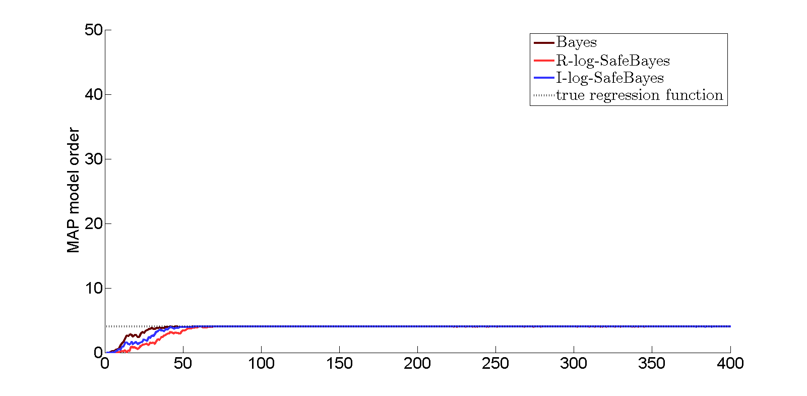
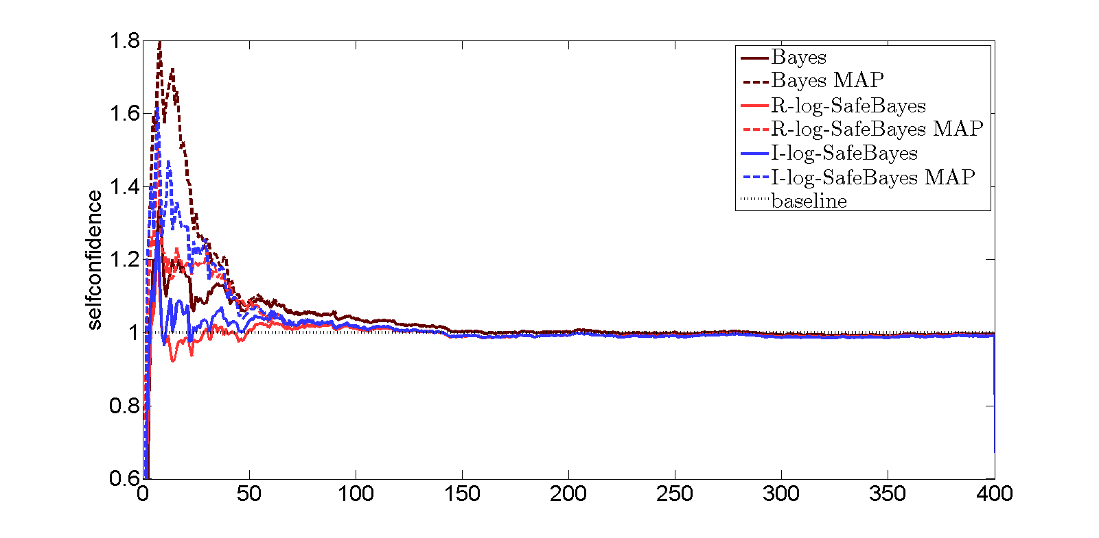
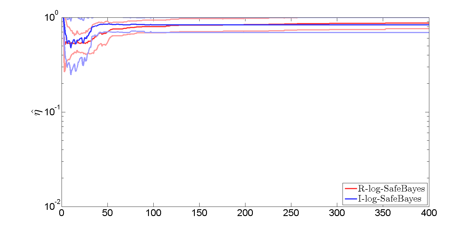
Figure 4: Same graphs as in Figure 3 for the correct-model experiment with $p_{\max}=50$.

Figure 5: Same four graphs as in Figure 3, for the wrong-model experiment with $p_{\max}=100$.

Figure 6: Same graphs as in Figure 3 for the correct-model experiment with $p_{\max}=100$.

5.4 Second Experiment: Ridge Regression, Varying $\sigma^{2}$

We repeat the model-wrong and model-correct experiment of Figure 3 and 4, with just one major difference: all posteriors are conditioned on $p:=p_{\max}=50$. Thus, we effectively consider just a fixed, high-dimensional model, whereas the best approximation $\tilde{\theta}=(50,\tilde{\beta},\tilde{\sigma}^{2})$ viewed as an element of $\mathcal{M}_{p}$ is ‘sparse’ in that it has only $\beta_{1},\ldots,\beta_{4}$ not equal to $0$. We note that the MAP model index graphs of Figure 3 and 4 are meaningless in this context (they would be equal to the constant 50) so they are left out of the new Figure 7 and  8.

Instantiating Safe Bayes

Since we noticed in preliminary experiments that some versions of SafeBayes now have a tendency to select much smaller values of $\eta$ than in the previous experiments, we now set $\kappa_{\max}=16$ (large enough so that in no experiment the optimal $\eta<2^{-\kappa_{\max}}$); for computational reasons we also increased the step size and set $\kappa_{\text{\sc step}}=1$.

Connection to Bayesian (B)ridge Regression

From (12) we see that the posterior mean parameter $\bar{\beta}_{i,\eta}$ is equal to the posterior MAP parameter and depends on $\eta$ but not on $\sigma^{2}$, since $\sigma^{2}$ enters the prior in the same way as the likelihood. Therefore, the square-loss obtained when using the generalized posterior for prediction is always given by $(y_{i}-x_{i}\bar{\beta}_{i,\eta})^{2}$ irrespective of whether we use the posterior mean, or MAP, or the value of $\sigma^{2}$. Interestingly, if we fix some $\lambda$ and perform standard (nongeneralized) Bayes with a modified prior, proportional to the original prior raised to the power $\lambda:=\eta^{-1}$, then the prior becomes normal $N(\bar{\beta}_{0},\sigma^{2}\Sigma^{\prime}_{0})$ where $\Sigma^{\prime}_{0}=\eta\Sigma_{0}$ and the standard posterior given $z^{i}$ is then (by (12)) Gaussian with mean

$$\left(\left(\Sigma^{\prime}_{0}\right)^{-1}+{\bf X}_{n}^{T}{\bf X}\right)^{-1}\cdot\left(\left(\Sigma^{\prime}_{0}\right)^{-1}\bar{\beta}_{0}+{\bf X}_{n}^{T}y^{n}\right)=\bar{\beta}_{i,\eta}.$$ (31)

Thus we see that in this special case, the (square-risk of the) $\eta$-generalized Bayes posterior mean coincides with the (square-risk of) the standard Bayes posterior mean with prior $N(\bar{\beta}_{0},\sigma^{2}\eta\Sigma_{0})$. But this means that the square-loss obtained by $\eta$-generalized Bayes on a data sequence is precisely equal to the square-loss obtained by Bayesian ridge regression with penalty parameter $\lambda=\eta^{-1}$, as defined, by, e.g., Park and Casella (2008) (to be precise, they call this method Bayesian ‘Bridge’ Regression with $q=2$; the choice of $q=1$ in their formula gives their celebrated ‘Bayesian Lasso’). It is thus of interest to see what happens if $\eta$ (equivalently, $\lambda$) is determined by empirical Bayes, which is one of the methods Park and Casella (2008) suggest. In addition to the graphs discussed earlier in Section 5.2, we thus also show the results for $\eta$ set in this alternative way. Whereas this empirical-Bayesian ridge regression is usually a very competitive method (indeed in our model-correct experiment, Figure 8, it performs best in al respects), we will see in Figure 7 (the green line) that, just like other versions of Bayes, it breaks down under our type of misspecification.

We hasten to add that the correspondence between the $\eta$-generalized posterior means and the standard posterior means with prior raised to power $1/\eta$ only holds for the $\bar{\beta}_{i,\eta}$ parameters. It does not hold for the $\bar{\sigma}^{2}_{i,\eta}$ parameters, and thus, for fixed $\eta$, the overconfidence of both methods may be quite different.

Figure 7: Bayesian Ridge Regression: Model-wrong experiment conditioned on $p:=p_{\max}=50$. The graphs (square-risk, overconfidence ratio and chosen $\eta$ as function of sample size) are as in Figure 3–6, except for the third graph there (MAP model order), which has no meaning here. The meaning of the curves is given in Section 5.2 except for empirical Bayes, explained in Section 5.4.

Figure 8: Bayesian Ridge Regression: same graphs as in Figure 7, but for the model-correct experiment conditioned on $p:=p_{\max}=50$.

Conclusions for Model-Wrong Experiment

For most curves, the overall picture of Figure 7 is comparable to the corresponding model averaging experiment, Figure 3: when the model is wrong, standard Bayes shows dismal performance in terms of risk and reliability up to a certain sample size and then very slowly recovers, whereas both versions of SafeBayes perform quite well even for small sample sizes. We do not show variations of the graph for $p=p_{\max}=100$ (i.e. the analogue of Figure 5), since it relates to Figure 7 in exactly the same way as Figure 5 relates to Figure 3: with $p=100$, bad square-risk and reliability behavior of Bayes goes on for much longer (recovery takes place at much larger sample size) and remains equally good as for $p=50$ with the two versions of SafeBayes.

The results for the Cesàro-versions of our methods are exactly as discussed at the end of Section 5.3.

We also see that, as we already indicated in the introduction, choosing the learning rate by empirical Bayes (thus implementing one version of Bayesian Bridge regression) behaves terribly. This complies with our general theme that, to ‘save Bayes’ in general misspecification problems, the parameter $\eta$ cannot be chosen in a standard Bayesian manner.

Conclusions for Model-Correct Experiment

The model-correct experiment for ridge regression (Figure 8) offers a surprise: we had expected Bayes to perform best, and were surprised to find that the SafeBayeses obtained smaller risk. Some followup experiments (not shown here), with different true regression functions and different priors, shed more light on the situation. Consider the setting in which the coefficients of the true function are drawn randomly according to the prior. In this setting standard Bayes performs at least as good in expectation as any other method including SafeBayes (the Bayesian posterior now represents exactly what an experimenter might ideally know). SafeBayes (still in this setting) usually chooses $\eta=1/2$ or $1/4$, and the difference in risks compared to Bayes is small. On the other hand, if the true coefficients are drawn from a distribution with substantially smaller variance than a priori expected by the prior (a factor 1000 in the ‘correct’-model experiment of Figure 8), then SafeBayes performs much better than Bayes. Here Bayes can no longer necessarily be expected to have the best performance (the model is correct, but the prior is “wrong”), and it is possible that a slightly reduced learning rate gives (significantly) better results. It seems that this situation, where the variance of the true function is much smaller than its prior expectation, is not exceptional: for example, Raftery et al. (1997) suggest choosing the variance of the prior in such a way that a large region of parameter values receives substantial prior mass. Following that suggestion in our experiments already gives a variance that is large enough compared to the true coefficients that SafeBayes performs better than Bayes even if the model is correct.

A Joint Observation for Model-Wrong and Model-Correct Experiment

Finally we note that we see an interesting difference between the two SafeBayes versions here: $I$-log-SafeBayes seems better for risk, giving a smooth decreasing curve in both experiments. $R$-log-SafeBayes inherits a trace of standard Bayes’ bad behavior in both experiments, with a nonmonotonicity in the learning curve. On the other hand, in terms of reliability, $R$-log-SafeBayes is consistently better than $I$-log-SafeBayes (but note that the latter is underconfident, which is arguably preferable over being overconfident, as Bayes is). All in al, there is no clear winner between the two methods.

5.5 Executive Summary: Joint Conclusions from Main and Additional Experiments

Standard Bayes

In almost all our experiments, Standard Bayesian inference fails in its KL-associated prediction tasks (squared risk, reliability) when the model is wrong. Adopting a different prior (such as the $g$-prior) does not help, with two exceptions in model averaging: (a) when Raftery’s prior (Section A.3) is used, then Bayes works quite well, but there it fails dramatically again (in contrast to SafeBayes) once the percentage of easy points is increased; (b) when it is run with a fixed variance that is significantly larger than the ‘best’ (pseudo-true) variance $\tilde{\sigma}^{2}$. Moreover, in the ridge regression experiment with fixed $\sigma^{2}$, we find that standard Bayes can even perform much worse than SafeBayes when the model is correct — so all in all we tentatively conclude that SafeBayes is safer to use for linear regression.

Safe Bayes

$R$-square-SafeBayes is not competitive with the other SafeBayes methods and can even get worse than Bayes sometimes; this is due to an unwanted dependence on the specified scale $\sigma^{2}$ as explained in Section A. The other three SafeBayes methods behave reasonably well in all our experiments, and there is no clear winner among them. $I$-square- SafeBayes usually behaves excellently for the square-risk but cannot directly be used to assess its own performance. $I$-log-SafeBayes usually behaves excellently in terms of square-risk as well but is underconfident about its own performance (which is perhaps acceptable, overconfidence being a lot more dangerous). $R$-log-SafeBayes is usually good in terms of square-risk though not as good as $I$-log-SafeBayes, yet it is highly reliable. However, in Appendix B.1, we describe an initial idea for discounting the importance of the first few outcomes and explain why this might improve performance. When combined with this discounting idea, $R$-log-SafeBayes may actually always be competitive with the other two methods in terms of square-risk as well.

Learning $\eta$ in Bayes- or Likelihood Way Fails

Despite its intuitive appeal, fitting $\eta$ to the data by e.g. empirical Bayes fails both in the model-wrong ridge experiment with a prior in $\sigma^{2}$, where it amounts to Bayesian ridge regression (Figure 7) and in the model-wrong fixed-variance ridge experiment (where it amounts to a method for learning the variance, see Section A.1.2).

Robustness of Experiments

It does not matter whether the $X_{i1},X_{i2},\ldots$ are independent Gaussian, uniform or represent polynomial basis functions: all phenomena reported here persist for all choices. If the ‘easy’ points are not precisely $(0,0)$, but have themselves a small variance in both dimensions, then all phenomena reported here persist, but on a smaller scale.

Centering

We repeated several of our experiments with centered data, i.e. preprocessed data so that the empirical average of the $Y_{i}$ is exactly 0 Raftery et al. (1997), Hastie et al. (2001). In none of our experiments did this affect any results. While this is not further mentioned in the appendix, there we also looked at the case where the true regression function has an intercept far from $0$, and data are not centered. This hardly affected the SafeBayes methods.

Other Methods

We also repeated the wrong-model experiment for other methods of model selection: AIC, BIC, and various forms of cross-validation. Briefly, we found that all these have severe problems with our data as well. Whereas in these experiments, cross-validation was used to identify a model index $p$ and $\eta$ played no role, in our final experiment we used leave-one-out cross-validation again to learn $\eta$ itself. With the squared error loss it worked fine, which is not too surprising given its close similarity to $I$-square-SafeBayes. However, when we tried it with log-loss (as a likelihoodist or information-theorist might be tempted to do), it behaved terribly.

6 Bayes’ Behavior Explained

In this section we explain how anomalous behavior of the Bayesian posterior may arise, taking a frequentist perspective. Section 6.1 is merely provided to give some initial intuition and may be skipped.

6.1 Explanation I: Variance Issues

Example 1

[Bernoulli] Consider the following very simple scenario: our ‘model’ consists of two Bernoulli distributions, $\mathcal{M}=\{P_{\theta}\mid\theta\in\{0.2,0.8\}\}$, with $P_{\theta}$ expressing that $Y_{1},Y_{2},\ldots\sim\text{i.i.d.~{}{\sc Ber}}(\theta)$. We perform Bayesian inference based on a uniform prior on $\mathcal{M}$. Suppose first that the data are, in fact, sampled i.i.d. from $P_{\theta^{*}}$, where $\theta^{*}$ is the ‘true’ parameter. The model is misspecified, in particular we will take a $\theta^{*}\not\in\{0.2,0.8\}$. The log-likelihood ratio between the two distributions for data $Y^{n}$ with $n_{1}$ ones and $n_{0}=n-n_{1}$ zeroes, measured for convenience in bits (base 2), is given by

$$L=\log_{2}\frac{{f}_{0.8}(Y^{n})}{{f}_{0.2}(Y^{n})}=\log_{2}\frac{(0.8)^{n_{1}}(0.2)^{n_{0}}}{(0.2)^{n_{1}}(0.8)^{n_{0}}}=2(n_{1}-n_{0}).$$ (32)

With uniform priors, the posterior will prefer $\theta=0.2$ as soon as $L<0$.

First suppose $\theta^{*}=1/2$. Then both distributions in $\mathcal{M}$ are equally far from $\theta^{*}$ in terms of KL divergence (or any other commonly used measure). By the central limit theorem, however, we expect that the probability that $|L|>\sqrt{n}/2$ is larger than a constant for all large $n$; in this particular case we numerically find that, for all $n$, it is larger than $0.32$.

This implies, that, at each $n$, with ‘true’ probability at least $0.32$, $\min_{\theta\in\{0.2,0.8\}}\pi(\theta\mid Y^{n})\approx 2^{-\sqrt{n}/2}$. Thus, there is a nonnegligible ‘true’ probability that the posterior on one of the two distributions is negligibly small, and a naive Bayesian who adopted such a model would be strongly convinced that the other distribution would be better even though both distributions are equally bad. While this already indicates that strange things may happen under misspecification, we are of course more interested in the situation in which $\theta^{*}\neq 1/2$, so that one of the two distributions in $\mathcal{M}$ is truly ‘better’. Now, if the ‘true’ parameter $\theta^{*}$ is within $O(1/\sqrt{n})$ of $1/2$, then, by the central limit theorem, the probability that $L<0$ is nonnegligible. For example, if $\theta^{*}$ is exactly $1/2+1/\sqrt{n}$, then this probability is larger than 0.16 for all $n$. Thus, for values of $\theta^{*}$ this close to $1/2$, there is no way we can even expect Bayes to learn the ‘best’ value. For fixed (independent of $n$), larger values of $\theta^{*}$, like $0.6$, the posterior will concentrate at $0.8$ at an exponential rate, but the sample size at which concentration starts is considerably larger than the sample sized needed when the true parameter is, in fact $0.8$. For example, at $n=50$, $P_{0.6}(L<0)\approx 0.1,P_{0.8}(L<0)\approx 2\cdot 10^{-5}$; both probabilities go to $0$ exponentially fast but their ratio increases exponentially with $n$. So, under a fixed $\theta^{*}$, with increasing $n$, Bayes may take longer to concentrate on the best $\tilde{\theta}$ if $\tilde{\theta}\neq\theta^{*}$ (misspecification) than if $\tilde{\theta}=\theta^{*}$, but it eventually ‘recovers’ (this was seen in the ridge experiments of Section 5.4). Now, for larger models, the consequence of slower concentration of the log-likelihood ratio $L$ is that the probability that some ‘bad’ $P_{\theta}$ happens to ‘win’ is substantially larger than with a correct model. Grünwald and Langford (2007) showed that, in a classification context with an infinite-dimensional model, there are so many of such ‘bad’ $P_{\theta}$ that Bayes does not recover any more, and the posterior keeps putting most of its mass on a bad model for ever (although the particular bad model on which it puts its mass, keeps changing). In this paper we empirically showed the same in a regression problem.

Now one might conjecture that the issues above are caused by the fact that the model $\mathcal{M}$ is ‘disconnected’. In the Bernoulli example above, the problem indeed goes away if instead of the model $\mathcal{M}$, we adopt its ‘closure’ $\mathcal{M}^{\prime}=\{P_{\theta}\mid\theta\in[0.2,0.8]\}$. However, high-dimensional regression problems exhibit the same phenomenon, even if their parameter spaces are connected. It turns out that in general, to get concentration at the same rates as if the model were correct, the model must be convex, i.e. closed under taking any finite mixture of the densities, which is a much stronger requirement than mere connectedness. For standard Gaussian regression problems with $Y\mid X\sim N(0,\sigma^{2})$, this would mean that we would have to adopt a model in which $Y\mid X$ can be any Gaussian mixture with arbitrarily many components — which is clearly not practical (note that ‘convex’ refers to the densities, not the regression functions (Grünwald and Langford, 2007, Section 6.3.5)).

6.2 Explanation II: Good vs. Bad Misspecification

Barron (1998) showed that sequential Bayesian prediction under a logarithmic score function shows excellent behavior in a cumulative risk sense; for a related result see (Barron et al., 1999, Lemma 4). Although Barron (1998) focuses on the well-specified case, this assumption is not required for the proof and the result still holds even if the model $\mathcal{M}$ is completely wrong. For a precise description and proof of this result emphasizing that it holds under misspecification, see (Grünwald, 2007, Section 15.2). At first sight, this leads to a paradox, as we now explain.

A Paradox?

Let $\tilde{\theta}$ index the KL-optimal distribution in $\Theta$ as in Section 2.1. The result of Barron (1998) essentially says that, for arbitrary models $\Theta$, for all $n$,

$$\mathbf{E}_{Z^{n}\sim P^{*}}\left[\sum_{i=1}^{n}\text{\sc risk}^{\text{log}}(\Pi\mid Z^{i-1})-\text{\sc risk}^{\text{log}}(\tilde{\theta})\right]\leq\text{\sc red}_{n},$$ (33)

where $\text{\sc risk}^{\text{log}}(W)$, for a distribution $W$ on $\Theta$, is defined as the log-risk obtained when predicting by the $W$-mixture of ${f}_{\theta}$, i.e.

$$\text{\sc risk}^{\text{log}}(W)=\mathbf{E}_{X,Y\sim P^{*}}[-\log\mathbf{E}_{\theta\sim W}{f}_{\theta}(Y\mid X)].$$ (34)

In (33), this coincides with log-risk of the Bayes predictive density $\bar{{f}}(\cdot\mid Z^{i-1})$, as defined by (3). Here, as in the remainder of this section, we look at the standard Bayes predictive density, i.e. $\eta=1$. $\text{\sc red}_{n}$ is the so-called relative expected stochastic complexity or redundancy (Grünwald, 2007), which depends on the prior and for ‘reasonable’ priors is typically small. The result thus means that, when sequentially predicting using the standard predictive distribution under a log-scoring rule, one does not lose much compared to when predicting with the log-risk optimal $\tilde{\theta}$.

When $\mathcal{M}$ is a union of a finite or countably infinite number of parametric exponential families and $\tilde{p}<\infty$ is well-defined, then, under some further regularity conditions, which hold in our regression example, Grünwald (2007), the redundancy is, up to $O(1)$, equal to the BIC term $(\tilde{k}/2)\log n$, where $\tilde{k}$ is the dimensionality of the smallest model containing $\tilde{\theta}$. In the regression case, $\mathcal{M}_{\tilde{p}}$ has $\tilde{p}+2$ parameters $(\beta_{0},\ldots,\beta_{p},\sigma^{2})$, so in the two experiments of Section 5, $\tilde{k}=6$. Thus, in our regression example, when sequentially predicting with the standard Bayes predictive $\bar{{f}}(\cdot\mid Z^{i-1})$, the cumulative log-risk is at most $n\cdot\text{\sc risk}^{\text{log}}(\tilde{\theta})$ which is linear in $n$, plus a logarithmic term that becomes comparatively negligible as $n$ increases. This is confirmed by Figure 10 below. Now, for each individual $\theta=(p,\beta,\sigma^{2})$ we know from Section 2.3 that, if its log-risk is close to that of $\tilde{\theta}$, then its square-risk must also be close to that of $\tilde{\theta}$; and $\tilde{\theta}$ itself has the smallest square-risk among all $\theta\in\Theta$. Hence, one would expect the reasoning for log-risk to transfer to square-risk: it seems that when sequentially predicting with the standard Bayes predictive $\bar{{f}}(\cdot\mid Z^{i-1})$, the cumulative square-risk should at most be $n$ times the instantaneous square-risk of $\tilde{\theta}$ plus a term that hardly grows with $n$; in other words, the cumulative square-risk from time $1$ to $n$, averaged over time by dividing by $n$, should rapidly converge to the constant instantaneous risk of $\tilde{\theta}$. Yet the experiments of Section 5 clearly show that this is not the case: Figure 3 shows that, until $n=100$, it is about 3 times as large.

This ‘paradox’ is resolved once we realize that the Bayesian predictive density $\bar{{f}}(\cdot\mid^{i-1})$ is a mixture of various ${f}_{\theta}$, and not necessarily similar to ${f}_{\theta}$ for any individual $\theta$ — the link between log-risk and square-risk (4) only holds for individual $\theta=(p,\beta,\sigma^{2})$, not for mixtures of them. Indeed, if at each point in time $i$, $\bar{{f}}(\cdot\mid Z^{i})$ would be very similar (in terms of e.g. Hellinger distance) to some particular ${f}_{\theta_{i}}$ with $\theta_{i}\in\Theta$, then there would really be a contradiction. Thus, the discrepancy between the good log-risk and bad square-risk results in fact implies that at a substantial fraction of sample sizes $i$, $\bar{{f}}(\cdot\mid Z^{i})$ must be substantially different from every $\theta\in\Theta$. In other words, the posterior is not concentrated at such $i$. A cartoon picture of this situation is given in Figure 9: the Bayes predictive achieves small log-risk because it mixes together several distributions into a single predictive distribution which is very different from any particular single ${f}_{\theta}\in\mathcal{M}$. By Barron’s bound, (33), the resulting $\bar{{f}}(\cdot\mid Z^{i})$ must, averaged over $i$, have at most a risk almost as small as the risk of $\tilde{\theta}$. We can thus, at least informally, distinguish between “benign” and “bad” misspecification. Bad misspecification occurs if there is a nonnegligible probability that for a range of sample sizes, the predictive distribution is substantially different from any of the distributions in $\mathcal{M}$. As Figure 9 suggests, ‘bad’ misspecification cannot occur for convex models $\mathcal{M}$ — and indeed, the results by Li (1999) suggest that for such models consistency holds under weak conditions for any $\eta<1$, even under misspecification.

6.3 Hypercompression

The picture suggests that, if, as in our regression model, the model is nonconvex (i.e. the set of densities $\{{f}_{\theta}\mid\theta\in\Theta\}$ is not closed under taking mixtures), then $\bar{{f}}(\cdot\mid Z^{i})$ might in fact be significantly better in terms of log-risk than the best $\tilde{\theta}$, and its individual constituents might even all be substantially worse than $\tilde{\theta}$. If this were indeed the case then, with high $P^{*}$-probability, we would also get the analogous result for an actual sample (and not just in expectation): the cumulative log-risk obtained by the Bayes predictive should be significantly smaller than the cumulative log-risk achieved with the optimal $\tilde{{f}}$. Figure 10 below shows that this indeed happens with our data, until $n\approx 100$.

The No-Hypercompression Inequality

In fact, Figure 10 shows a phenomenon that is virtually impossible if the Bayesian’s model and prior are ‘correct’ in the sense that data $Z^{n}$ would behave like a typical sample from them: it easily follows from Markov’s inequality (for details see (Grünwald, 2007, Chapter 3)) that, letting $\Pi$ denote the Bayesian’s joint distribution on $\Theta\times\mathcal{Z}^{n}$, for each $K\geq 0$,

$$\Pi\left\{(\theta,Z^{n})\ :\ \sum_{i=1}^{n}\left(-\log\bar{{f}}(Y_{i}\mid X_{i},Z^{i-1})\right)\leq\sum_{i=1}^{n}\left(-\log{f}_{\theta}(Y_{i}\mid X_{i},Z^{i-1})\right)-K\right\}\leq e^{-K},$$

i.e. the probability that the Bayes predictive $\bar{{f}}$ cumulatively outperforms ${f}_{\theta}$, with $\theta$ drawn from the prior, by $K$ log-loss units is exponentially small in $K$. Figure 10 below thus shows that at sample size $n\approx 90$, an a-priori formulated event has happened of probability less than $e^{-30}$, clearly indicating that something about our model or prior is quite wrong.

Since the difference in cumulative log-loss between $\bar{{f}}$ and ${f}_{\theta}$ can be interpreted as the amount of bits saved when coding the data with a code that would be optimal under $\bar{{f}}$ rather than ${f}_{\theta}$, this result has been called the no hyper-compression inequality by Grünwald (2007). The figure shows that for our data, we have substantial hypercompression.

Figure 9: Benign vs. Bad Misspecification: $\tilde{P}=\arg\min_{P\in\mathcal{M}}D(P^{*}\|P)$ is the distribution in model $\mathcal{M}$ that minimizes KL divergence to the ‘true’ $P^{*}$, but, since the model is nonconvex, the Bayes predictive distribution $\bar{P}$ may happen to be very different from any $P\in\mathcal{M}$. When this happens, we can have ‘bad misspecification’ and then it may be necessary to decrease the learning rate (in this simplistic drawing $\bar{P}$ is a mixture of just two distributions; in our regression example it mixes infinitely many). Yet if $P^{*}$ were such that $\inf_{P\in\mathcal{M}}D(P^{*}\|P)$ does not decrease if the infimum is taken over the convex hull of $\mathcal{M}$ (e.g. if $Q$ rather than $\tilde{P}$ reached the minimum), then any learning rate $\eta<1$ is fine (‘benign’ misspecification). In the picture, we even have $D(P^{*}\|\bar{P})<D(P^{*}\|\tilde{P})$; in this case we can get hypercompression.

The Safe Bayes Error Measure

As seen from (18), SafeBayes measures the performance of $\eta$-generalized Bayes not by the cumulative log-loss, as standard Bayes does, but instead by the cumulative posterior-expected error when predicting by drawing from the posterior. One way to interpret this alternative error measure is that, at least in expectation, we cannot get hypercompression. Defining (compare to (34)!)

$$\text{\sc risk}^{\text{R-log}}(W)=\mathbf{E}_{X,Y\sim P^{*}}E_{\theta\sim W}[-\log{f}_{\theta}(Y\mid X)],$$ (35)

we get by Fubini’s theorem,

$$\text{\sc risk}^{\text{R-log}}(W)-\text{\sc risk}^{\text{log}}(\tilde{\theta})=E_{\theta\sim W}\mathbf{E}_{X,Y\sim P^{*}}[[-\log{f}_{\theta}(Y\mid X)]-[-\log{f}_{\tilde{\theta}}(Y\mid X)]]\geq 0,$$ (36)

where the inequality follows by definition of $\tilde{\theta}$ being log-risk optimal among $\Theta$. There is thus a crucial difference between $\text{\sc risk}^{\text{R-log}}$ and $\text{\sc risk}^{\text{log}}$ — for the latter we just argued that, under misspecification, $\text{\sc risk}^{\text{log}}(W)-\text{\sc risk}^{\text{log}}(\tilde{\theta})\leq 0$ is very well possible. Thus, in contrast to predicting with the mixture density $\mathbf{E}_{\theta\sim W}f_{\theta}$, prediction by randomization (first sampling $\theta\sim W$ and then predicting with the sampled $f_{\theta}$) cannot ‘exploit’ the fact that mixture densities might have smaller log-risk than their components. Thus, if the difference (36) is small, then $W$ must put most of its mass on distributions $\theta\in\Theta$ that have small log-risk themselves. For individual $\theta$, we know that small log-risk implies small square- risk. This implies that if (36) is small, then the (standard) posterior is concentrated on distributions with small $R$-square-risk.

Experimental Demonstration of Hypercompression for Standard Bayes

Figure 10 and Figure 11 show the predictive capabilities of Standard Bayes in the wrong model example in terms of cumulative and instantaneous log-loss on a simulated sample. The graphs clearly demonstrate hypercompression: the Bayes predictive cumulatively performs better than the best single model/the best distribution in the model space, until at about $n\approx 100$ there is a phase transition. At individual points, we see that it sometimes performs a little worse, and sometimes (namely at the ‘easy’ $(0,0)$ points) much better than the best distribution. We also see that, as anticipated above, randomized and in-model Bayesian prediction do not show hypercompression and in fact perform terribly on the log-loss until the phase transition at $n=100$, when they becomes almost as good as standard Bayes. We see that for $\eta=1$, they perform much worse. An important conclusion is that if we are only interested in log-loss prediction, it is clear that we just want to use Bayes rather than randomized or in-model prediction with different $\eta$.

As an aside, we note that the first few outcomes have a dramatic effect on cumulative $R$-and $I$-log-loss (it disappears from Figure 11); this may be due to the fact that our densities — other than those considered by Grünwald (2012) — have unbounded support so that there is no $v$ such that Theorem 1 below holds. This observation inspired the idea described in Appendix B.1 about ignoring the first few outcomes when determining the optimal $\eta$. Also, we emphasize that the hypercompression phenomenon takes places more generally, not just in our regression setup — for example, the classification inconsistency noted by Grünwald and Langford (2007) can be understood in terms of hypercompression as well.

Figure 10: Cumulative standard, $R$-, and $I$-log-Loss as defined in (18) and (22) respectively of standard Bayesian prediction ($\eta=1$) on a single run for the model-averaging experiment of Figure 3. We clearly see that standard Bayes achieves hypercompression, being better than the best single model. And, as predicted by theory, randomized Bayes is never better than standard Bayes, whose curve has negative slope because the densities of outcomes are $>1$ on average.

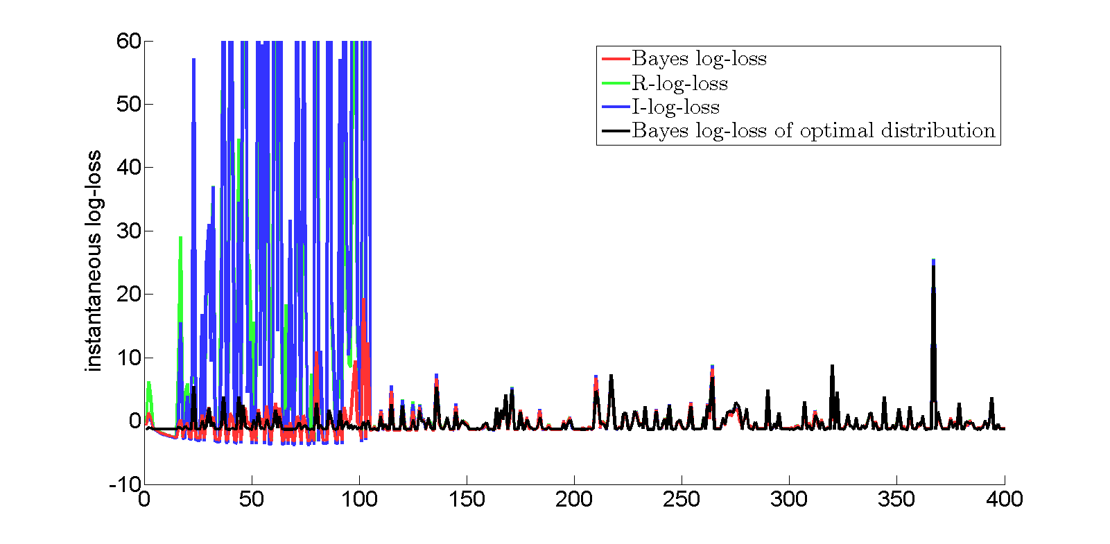
Figure 11: Instantaneous standard, $R$- and $I$-log-Loss of standard Bayesian prediction for the run depicted in Figure 10.

How Hypercompression arises in Regression

Figure 12 gives some clues as to how hypercompression is achieved: it shows the variance of the predictive distribution $\bar{{f}}(\cdot\mid Z^{50})$ as a function of $S\in[-1,1]$ for the polynomial example of Figure 1 in the introduction, at sample size $n=50$, where hypercompression takes place. Figure 1 gave the posterior mean (regression function) at $n=100$; the function at $n=50$ looks similar, correctly having mean $0$ at $S=0$ but, incorrectly, mean far from $0$ at most other $S$. The predictive distribution conditioned on the MAP model ${\cal M}_{\breve{p}_{\text{map}(Z^{50})}}$ is a t-distribution with approximately $\breve{p}_{\text{map}(Z^{50})}\approx 50$ degrees of freedom, which means that it is approximately normal. Figure 12 shows that its variance is much smaller than the variance $\tilde{\sigma}^{2}$ at $S=0$; as a result, its log-risk conditional on $U=0$ is smaller than that of $\tilde{\theta}=(\tilde{p},\tilde{\beta},\tilde{\sigma}^{2})$ by some large amount $A$. Conditioned at $S\neq 0$, its conditional mean is off by some amount, and its variance is, on average, slightly (but not much) smaller than $\tilde{\sigma}^{2}$, making its conditional log-risk given $U\neq 0$ larger than that of $\tilde{\theta}$ by an amount $A^{\prime}$ where, it turns out, $A^{\prime}$ is smaller than $A$. Both events $S=0$ and $S\neq 0$ happen with probability $1/2$, so that the final, unconditional log-risk of $\bar{{f}}(\cdot\mid Z^{50})$ is smaller than that of $\tilde{\theta}$.

Summarizing, hypercompression occurs because the variance of the predictive distribution conditioned on past data and a new $X$ is much smaller than $\tilde{\sigma}^{2}$ at $X=0$. This suggests that, if instead of a prior on $\sigma^{2}$ we use models $\mathcal{M}_{p}$ with a fixed $\sigma^{2}$, we can only get hypercompression (and correspondingly bad square-risk behaviour) if $\sigma^{2}\ll\tilde{\sigma}^{2}$, because the predictive variance based on linear models $\mathcal{M}_{p}$ with fixed variance $\sigma^{2}$ given $X=x$ is, for all $x$, lower bounded by $\sigma^{2}$. Our experiments in Appendix A.1 confirm that this is indeed what happens.

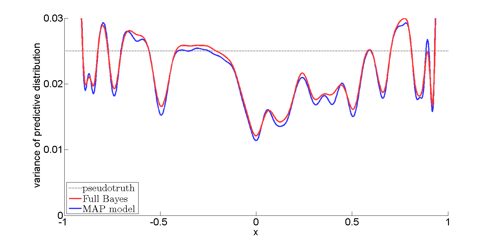
Figure 12: Variance of standard Bayes predictive distribution conditioned on a new input $S$ as a function of $S$ after 50 examples for the model-wrong experiment (Figure 3), shown both for the predictive distribution based on the full, model-averaging posterior and for the posterior conditioned on the MAP model ${\cal M}_{\breve{p}_{\text{map}}}$. For both posteriors, the posterior mean of $Y$ is incorrect for $x\neq 0$, yet $\bar{{f}}(Y\mid Z^{50},X)$ still achieves small risk because of its small variance at $X=0$.

6.4 Explanation III: The Mixability Gap & The Bayesian Belief in Concentration

As we indicated at the end of Section 6.2, bad misspecification can occur only if the standard ($\eta=1$) posterior is nonconcentrated. Intriguingly, by formalizing ‘concentration’ in the appropriate way, we will now show, under some conditions on the prior, that a Bayesian a priori always believes that the posterior will concentrate very fast. Thus, if we observe data $Z^{n}$, and for many $n^{\prime}\leq n$, the posterior based on $Z^{n^{\prime}}$ is not concentrated, then we can view this as an indication of bad misspecification. In the next subsection we will see that SafeBayes selects a $\hat{\eta}\ll 1$ iff we have such nonconcentration at $\eta=1$. Thus, SafeBayes can partially be understood as a prior predictive check, i.e. a test whether the assumptions implied by the prior actually hold on the data (Box, 1980).

The Mixability Gap

We express posterior nonconcentration in terms of the mixability gap (Grünwald, 2012, de Rooij et al., 2014). In this section we only consider the special case of $\eta=1$ (standard Bayes), for which the mixability gap $\delta_{i}$ is defined as the difference between $1$-$R$-log-loss (18) and standard log-loss as obtained by predicting with the posterior predictive, at sample size $i$:

$$\delta_{i} :=\mathbf{E}_{\theta\sim\Pi\mid z^{i-1}}\left[-\log{f}(y_{i}\mid x_{i},\theta)\right]-\left(-\log\mathbf{E}_{\theta\sim\Pi\mid z^{i-1}}[{f}(y_{i}\mid x_{i},\theta)]\right)$$

$$\;=\mathbf{E}_{\theta\sim\Pi\mid z^{i-1}}\left[-\log{f}_{\theta}(y_{i}\mid x_{i})\right]-\left(-\log\bar{{f}}(y_{i}\mid x_{i},z^{i-1})\right),$$ (37)

Straightforward application of Jensen’s inequality as in (19) gives that $\delta_{i}\geq 0$. $\delta_{i}$, which depends on $z_{1},\ldots,z_{i}$, is a measure of the posterior’s concentratedness at sample size $i$ when used to predict $y_{i}$ given $x_{i}$: it is small if ${f}_{\theta}(y_{i}\mid x_{i})$ does not vary much among the $\theta$ that have substantial $\eta$-posterior mass; by strict convexity of $-\log$, it is $0$ iff there exists a set $\Theta_{0}$ with $\Pi(\Theta_{0}\mid Z^{i-1})=1$ such that for all $\theta,\theta^{\prime}\in\Theta_{0}$, $f_{\theta}(y_{i}\mid x_{i})=f_{\theta^{\prime}}(y_{i}\mid x_{i})$.

We set the cumulative mixability gap to be $\Delta_{n}:=\sum_{i=1}^{n}\delta_{i}$.

The Bayesian Belief in Posterior Concentration

As a theoretical contribution of this paper, we now show that, under some conditions on model and prior, if the data are as expected by the model and prior, then the expected mixability gap goes to $0$ as $O((\log n)/n)$, and hence a Bayesian automatically a priori believes that the posterior will concentrate fast. For simplicity we restrict ourselves to a model $\mathcal{M}=\{P_{\theta}:\theta\in\Theta\}$ where $\Theta$ is countable, and we let all $\theta\in\Theta$ represent a conditional distribution for $Y$ given $X$, extended to $n$ outcomes by independence. We let $\pi$ be a probability mass on $\Theta$, and define the joint Bayesian distribution $\Pi$ on $\Theta\times\mathcal{Y}^{n}\mid\mathcal{X}^{n}$ in the usual way, so that for measurable $\mathcal{A}\subset\mathcal{Y}^{n}$, $\Pi((\theta^{*},\mathcal{A})\mid X^{n}=x^{n})=\pi(\theta^{*})\cdot P_{\theta^{*}}(\mathcal{A}\mid X^{n}=x^{n})$. The random variable $\theta^{*}$ refers to the $\theta$ chosen according to density $\pi$. We will look at the Bayesian probability distribution of the $\theta^{*}$-expected mixability gap, $\bar{\delta}_{n}:=\mathbf{E}_{\theta^{*}}[\delta_{n}]$.

Theorem 1

Consider a countable model with prior $\Pi$ as above. Suppose that the density ratios in $\Theta$ are uniformly bounded, i.e. there is a $v>1$ such that for all $x,y\in\mathcal{X}\times\mathcal{Y}$, all $\theta,\theta^{\prime}\in\Theta$, ${f}_{\theta}(y\mid x)/{f}_{\theta^{\prime}}(y\mid x)\leq v$. Suppose that for some $\eta<1$ we have $\sum_{\theta}\pi(\theta)^{\eta}<\infty$. Then for every $a>0$ there are constants $C_{0}$ and $C_{1}$ such that, for all $n$,

$$\Pi\left(\ \bar{\delta}_{n}\geq C_{0}\cdot\frac{\log n}{n}\ \right)\leq C_{1}\cdot\frac{1}{n^{a}}.$$ (38)

Moreover, for any $0<a^{\prime}\leq 1$, there exist $C_{2}$ and $C_{3}$ such that

$$\Pi\left(\ {\Delta}_{n}\geq C_{2}\cdot n^{a^{\prime}}\ \right)\leq C_{3}\cdot\frac{(\log n)^{2}}{n^{a^{\prime}}},$$ (39)

i.e. the Bayesian believes that the mixability gap will be small on average and that the cumulative mixability gap will be small with high probability.

Thus, with high probability, $\Delta_{n}$ grows only polylogarithmically, even though it is the difference of two quantities that are typically linear in $n$. This means that observing a large value of $\Delta_{n}$ strongly indicates misspecification.

• We hasten to add that the regularity conditions for Theorem 1 do not hold in the regression problem we study in this paper; the theorem is merely meant to show that $\Delta_{n}$ is believed to be small in idealized circumstances that have been simplified so as to make mathematical analysis easier. Note however, that the regularity conditions do not constrain $\Theta$ in the most important respect: by allowing countably infinite $\Theta$, we can approximate nonparametric models arbitrarily well by suitable covers (Barron and Cover, 1991). In particular we do allow sets $\Theta$ for which maximum likelihood methods would lead to disastrous overfitting at all sample sizes. Also the condition that $\sum\pi(\theta)^{\eta}<\infty$ is standard in proving Bayesian and MDL convergence theorems (Barron and Cover, 1991, Zhang, 2006a). In fact, since the constants $C_{0}$ and $C_{1}$ scale logarithmically in $v$, we expect that Theorem 1 can be extended to the regression setting we are dealing with here as long as all distributions in the model have exponentially small tails, using methods similar to those in Grünwald and Mehta (2016).

Example 2

[Cumulative Nonconcentration can (and will) go together with Momentary Concentration: Example 1, Bernoulli, Cont.] Consider the first instance of the Bernoulli Example 1 again, where we again look at what happens if both distributions are equally bad: $\mathcal{M}=\{P_{0.2},P_{0.8}\}$, whereas $Y_{1},Y_{2},\ldots$ are i.i.d. $\sim P_{\theta^{*}}$ with $\theta^{*}=1/2$. As we showed in that example, at any given $n$, with $P_{\theta^{*}}$-probability at least $0.32$, $\min_{\theta\in\{0.2,0.8\}}\pi(\theta\mid Y^{n})\approx 2^{-\sqrt{n}/2}$: the posterior puts almost all mass on one $\theta$. Lemma 6 of van Erven et al. (2011) shows that in such cases $\delta_{n}$ is small; in this particular case, $\delta_{n}\leq 2(e-2)\min_{\theta\in\{0.2,0.8\}}\pi(\theta\mid Y^{n})\approx 1.42\cdot 2^{-\sqrt{n}/2}$. Thus, the posterior looks exceedingly concentrated at time $n$, with nonnegligible probability (this unwarranted confidence is a simplified version of what was called the fair balance paradox by Yang (2007), who conjectured it is the underlying reason for the problem of ‘overconfident posteriors’ in Bayesian phylogenetic tree inference). However, Safe Bayes detects misspecification by looking at cumulative concentration, i.e. the sum of the $\delta$’s: $L$ as in (32) can be interpreted as a random walk on ${\mathbb{Z}}$ starting at the origin, with equal probabilities to move to the left and to the right. By the central limit theorem, the random walk crosses the origin at time $n$ with probability about $1/\sqrt{n\pi/2}=\tilde{O}(n^{-1/2})$, so that we may conjecture that, with high probability, it crosses the origin $\tilde{O}(n\cdot n^{-1/2})=\tilde{O}(n^{1/2})$ times. Each time it crosses the origin, the posterior is uniform and hence as nonconcentrated as it can be, and $\Delta_{n}$ is increased by at least a fixed constant. One would therefore expect (under the ‘true’ $\theta^{*}$) that $\Delta_{n}$ is of order $\sqrt{n}$, which by Theorem 1 is much larger than a Bayesian a priori expect it to be — the model fails the ‘prior predictive check’.

6.5 How Safe Bayes Works

In its simplest form, the in-model fixed variance case, SafeBayes finds the $\hat{\eta}$ that minimizes cumulative square-loss on the sample and thus can simply be understood as a pragmatic attempt to find a $\hat{\eta}$ that achieves small risk. However, the other versions of SafeBayes do not have such an easy interpretation. To explain them further, we need to generalize the notion of mixability gap in terms of the $\eta^{\prime}$-flattened $\eta$-generalized Bayesian predictive density. The latter is defined, for $\eta,\eta^{\prime}\leq 1$, as:

$$\bar{{f}}(y_{i}\mid x_{i},z^{i-1},\langle\eta^{\prime}\rangle;\eta):=\left(\mathbf{E}_{\theta\sim\Pi\mid z^{i-1},\eta}\left[{f}_{\theta}^{\eta^{\prime}}(y_{i}\mid x_{i})\right]\right)^{1/\eta^{\prime}}.$$ (40)

By Jensen’s inequality, for any $\eta^{\prime}\leq 1$, any $(x_{i},y_{i})$, we have $\bar{{f}}(y_{i}\mid x_{i},z^{i-1},\langle\eta^{\prime}\rangle;\eta)\leq\bar{{f}}(y_{i}\mid x_{i},z^{i-1},\eta)$. Indeed, intentionally, $\bar{{f}}(\cdot\mid\langle\eta^{\prime}\rangle;\eta)$ is a ‘defective’ density in the sense that $\int_{{\mathbb{R}}}\bar{{f}}(y\mid x_{i},z^{i-1},\langle\eta^{\prime}\rangle;\eta)dy<1$. The log-loss achieved by $\eta$-generalized, $\eta^{\prime}$-flattened Bayesian prediction is called $(\eta,\eta^{\prime})$-mix-loss from now on, following terminology from de Rooij et al. (2014). For $0<\eta\leq\eta^{\prime}\leq 1$, the mixability gap $\delta_{i,\eta,\eta^{\prime}}$ is defined as the difference between the $\eta$-$R$-log-loss and the $\eta^{\prime}$-mix-loss:

$$\delta_{i,\eta,\eta^{\prime}}:=\mathbf{E}_{\theta\sim\Pi\mid Z^{i-1},\eta}\left[-\log{f}_{\theta}(Y_{i}\mid X_{i})\right]-\left(-\log\bar{{f}}(Y_{i}\mid X_{i},Z^{i-1};\langle\eta^{\prime}\rangle;\eta)\right).$$ (41)

We once again define a cumulative version $\Delta_{n,\eta,\eta^{\prime}}=\sum_{i=1}^{n}\delta_{i,\eta,\eta^{\prime}}$, and note that the definitions are compatible with the special cases $\delta_{i}:=\delta_{i,1,1}$ and $\Delta_{n}:=\Delta_{n,1,1}$ defined in the previous subsection. Now we can rewrite the cumulative $R$-log-loss achieved by Bayes with the $\eta$-generalized posterior as

$$\sum_{i=1}^{n}\mathbf{E}_{\theta\sim\Pi\mid z^{i-1},\eta}\left[-\log{f}_{\theta}(y_{i}\mid x_{i})\right]=\Delta_{n,\eta,\eta^{\prime}}+\text{CML}_{n,\eta,\eta^{\prime}},$$ (42)

where

$$\text{CML}_{n,\eta,\eta^{\prime}}=\left(\sum_{i=1}^{n}-\log\bar{{f}}(y_{i}\mid x_{i},z^{i-1},\langle\eta^{\prime}\rangle;\eta)\right)$$

is the cumulative $(\eta,\eta^{\prime})$-mix-loss. (42) holds for all $0<\eta\leq\eta^{\prime}\leq 1$. Consider first $\eta^{\prime}=1$. As was seen, if $\Delta_{n,1,1}$ is large, then this indicates potential bad misspecification. But (42) still holds for smaller $\eta^{\prime}<1$; by Jensen’s inequality, for any fixed $\eta$, decreasing $\eta^{\prime}$ will make $\Delta_{n,\eta,\eta^{\prime}}$ smaller as well. Indeed, for any fixed $P^{*}$, defining

$$\bar{\delta}_{\eta^{\prime}}:=\sup_{W}\;\mathbf{E}_{X,Y\sim P^{*}}\left[\;\mathbf{E}_{\theta\sim W}[-\log{f}_{\theta}(Y\mid X)]-\left(-\frac{1}{\eta^{\prime}}\log\mathbf{E}_{\theta\sim W}[{f}_{\theta}(Y\mid X)^{\eta^{\prime}}]\right)\right],$$

where the supremum is over all distributions on $\Theta$, we have

$$\lim_{\eta^{\prime}\downarrow 0}\bar{\delta}_{\eta^{\prime}}=0,$$

so we have an upper bound on the expectation of $\Delta_{n,\eta,\eta^{\prime}}$ independent of the actual data that, for small enough $\eta^{\prime}$, will become negligibly small. But the left-hand side of (42) does not depend on $\eta^{\prime}$, so if, by decreasing $\eta^{\prime}$, we decrease $\Delta_{n,\eta,\eta^{\prime}}$, $\text{CML}_{n,\eta,\eta^{\prime}}$ must increase by the same amount — so as yet we have gained nothing. Indeed, not surprisingly, Barron’s bound does not hold any more for $\text{CML}_{n,\eta,\eta^{\prime}}$ with $\eta=1$ and $\eta^{\prime}<1$ (and in general, it does not hold for $\eta,\eta^{\prime}$ whenever $\eta^{\prime}<\eta$). But, it turns out, a version of Barron’s bound still holds for $\text{CML}_{n,\eta^{\prime},\eta^{\prime}}$, for all $\eta^{\prime}>0$: the cumulative log-risk of $\eta^{\prime}$-flattened, $\eta^{\prime}$-generalized Bayes is still guaranteed to be within a small $\text{\sc red}_{n}$ of the cumulative log-risk of $\tilde{\theta}$, although $\text{\sc red}_{n}$ does monotonically increase as $\eta^{\prime}$ gets smaller — simply because the prior becomes more important relative to the data (standard results in learning theory show that $\text{CML}_{n,\eta,\eta}$ is monotonically decreasing in $\eta$, and can be upper bounded as $O(1/\eta)$; see e.g. (de Rooij et al., 2014, Lemma 1). Thus, it makes sense to consider the special case $\eta^{\prime}=\eta$, and think of SafeBayes as finding the $\eta$ minimizing

$$\sum_{i=1}^{n}\mathbf{E}_{\theta\sim\Pi\mid z^{i-1},\eta}\left[-\log{f}_{\theta}(y_{i}\mid x_{i})\right]=\Delta_{n,\eta,\eta}+\text{CML}_{n,\eta,\eta},$$ (43)

since we have clear interpretations of both terms: the second indicates, by Barron’s bound, how much worse the $\eta$-generalized posterior predicts in terms of log-loss compared to the optimal $\tilde{\theta}$; the first indicates how much is additionally lost if one is forced to predict by distributions inside the model. The second term decreases in $\eta$, the first has an upper bound which increases in $\eta$. SafeBayes can now be understood as trying to minimize both terms at the same time.

Now broadly speaking, the central convergence result of Grünwald (2012) states that $\Delta_{n,\eta,\eta}$ will be ‘sufficiently small’ for all $\eta<1$, and under some further conditions even for $\eta=1$, if the model is correct or convex; and it will also be ‘sufficiently small’ if the model is incorrect, as long as $\eta$ is smaller than some ‘critical’ value $\eta_{\text{crit}}$ (which may depend on $n$ though). Here ‘sufficiently small’ means that it is not the dominating term in (43). Intuitively, we would like the $\hat{\eta}$ determined by SafeBayes to be the largest $\eta$ that is smaller than $\eta_{\text{crit}}$. Grünwald (2012) shows that Safe Bayes indeed finds such an $\eta$, and that prediction based on the generalized posterior with this $\eta$ achieves good frequentist convergence rates.

Experimental Illustration:

Consider the main wrong-model experiment of Section 5. Figure 13 shows, as a function of $\eta$, in red, the cumulative $\eta$-$R$-log-loss achieved by Safe Bayes, averaged over 30 runs of Experiment 1 (Bayesian model averaging with incorrect model) of Figure 3. In each individual run, Safe Bayes picks the $\hat{\eta}$ minimizing this quantity; we thus get that on most runs, $\hat{\eta}$ is close to $0.4$. In contrast to $\eta$-$R$-log-loss, and as predicted by theory, the $\eta$-mix-loss (in purple) decreases monotonically and coincides with the standard Bayesian log-loss at $\eta=1$ and with the $\eta$-$R$-log-loss as $\eta\downarrow 0$. We also see hypercompression again: near $\eta=1$, both the Bayesian log-loss and the mix-loss are smaller than the log-loss achieved by the best $\tilde{\theta}$ in the model. At $\eta=0.5$, there is a sudden sharp rise in $\Delta_{n,\eta,\eta}$ (the difference between the red and purple curves). We can think of Safe Bayes as trying to identify this ‘critical’ $\eta_{\text{crit}}$.

Figure 13: Cumulative losses up to sample 100 (where the posterior has not converged yet) as a function of $\eta$, averaged over 30 runs, for the experiment of Figure 3. $\eta$-B-log-loss is the cumulative log-loss achieved by standard Bayes with the $\eta$-generalized posterior.

• Theorem 1 shows that, if both model and prior are well-specified, then the Bayesian posterior cumulatively concentrates in a very strong sense. More generally, if the model is correct but also if there is ‘benign’ misspecification, then, under some conditions on the prior, by the results of Grünwald (2012), the Bayesian posterior eventually cumulatively concentrates at $\eta=1$. One might thus be tempted to interpret $\eta_{\text{crit}}$ (the learning rate which SafeBayes tries to learn) as ‘largest learning rate at which the posterior cumulatively concentrates’. However, this interpretation works only if $\eta_{\text{crit}}=1$. If $\eta_{\text{crit}}<1$, we can only show that, for every $\eta<\eta_{\text{crit}}$, $\Delta_{n,\eta,\eta}$ is small; true cumulative concentration would instead mean that $\Delta_{n,\eta,1}$ is small for such $\eta$ (note we must have $\Delta_{n,\eta,\eta}\leq\Delta_{n,\eta,1}$ by Jensen). The figure shows that $\Delta_{n,\eta,1}$ (the difference between the red and blue curve) may indeed be large even at small $\eta$. A better interpretation is that, for every fixed $\eta$, with decreasing $\eta^{\prime}$, the geometry of the $(\eta,\eta^{\prime})$-mix-loss changes, so that the loss difference between the mix loss and the $R$-log-loss obtained by randomization gets smaller. By then further using the generalized posterior for the same $\eta^{\prime}$, we guarantee that a version of Barron’s bound holds for the $(\eta^{\prime},\eta^{\prime})$-mix-loss.

• Replacing $R$- by $I$-loss Although the proofs of Grünwald (2012) are optimized for $R$-SafeBayes, the same story as above can be told for any fixed transformation from the posterior to a possibly randomized prediction, i.e. anything of the form (21); in particular for the most extreme transformation where we replace the posterior predictive by the distribution indexed by the posterior mean parameters so that instead of $R$-SafeBayes we end up with $I$-SafeBayes. In fact, the importance of the distinction between ‘in-model’ and ‘out-model’ prediction under model misspecification has been emphasized before (Grünwald, 2007, Barron and Hengartner, 1998, Kotłowski et al., 2010). In general, although we do not know how to exploit this intuition to strengthen the convergence proofs of Grünwald (2012), it seems more natural to replace the randomized predictions by deterministic, in-model predictions.

7 Discussion, Open Problems and Conclusion

“If a subjective distribution $\Pi$ attaches probability zero to a non-ignorable event, and if this event happens, then $\Pi$ must be treated with suspicion, and modified or replaced” (emphasis added)
— A.P. Dawid (1982).

“Some models are obviously wrong, yet evidently useful”
— (very freely paraphrasing Box (1979)).

We already discussed the theoretical significance of the inconsistency result in the introduction. Extensive further discussion on Bayesian inference under misspecification is given by Walker (2013) and Grünwald and Langford (2007). For us, it remains to discuss the place of both the inconsistency result and our solution in Bayesian methodology.

Following the well-known Bayesian statisticians Box (1980), Good (1983), Dawid (1982, 2004) and Gelman (2004) (see also Gelman and Shalizi (2012)), we take the stance that model checking is a crucial part of successful Bayesian practice. When there is a large discrepancy between a model’s predictions and actual observations, it is not merely sufficient to keep gathering data and update one’s posterior: something more radical is needed. In many such cases, the right thing to do is to go back to the drawing board and try to devise a more realistic model. However, we think this story is incomplete: in machine learning and pattern recognition, one often encounters situations in which the model employed is obviously wrong in some respects, yet there is a model instantiation (parameter vector) that is pretty adequate for the specific prediction task one is interested in. Examples of such obviously-wrong-yet-pretty-adequate models are, like in this paper, assuming homoskedasticity in linear regression when the goal is to approximate the true regression function and the true noise is heteroskedastic, but also the use of $N$-grams in language modeling (is the probability of a word given the previous three words really independent of everything that was said earlier?), logistic regression in e.g. spam filtering, and every single successful data compression method that we know of (see Bayes and Gzip (Grünwald, 2007, Chapter 17, page 537)). The difference with the more standard statistical (be it Bayesian or frequentist) mode of reasoning is eloquently described in Breiman’s (2001) the two cultures. Bayesian inference is among the most successful methods currently used in the obviously-wrong-yet-pretty-adequate-situation (to witness, state-of-the-art data compression methods such as Context-Tree-Weighting Willems et al. (1995) have a Bayesian interpretation). Yet the present paper shows that there is a danger: even if the employed model is pretty adequate (in the sense of containing a pretty good predictor), the Bayesian machinery might not be able to find it. The Safe Bayesian algorithm can thus be viewed as an attempt to provide an alternative for the data-analysis cycle (Gelman and Shalizi, 2012) to this, in some sense, less ambitious setting: just like in the standard cycle, we do a model check, albeit a very specific one: we check whether there is ‘cumulative concentration of the posterior’ (see Section 6.4). If there is not, we know that we may not be learning to predict as well as the best predictor in our model, so we modify our posterior. Not in the strong sense of ‘going back to the drawing board’, but in the much weaker sense of making the learning rate smaller — we cannot hope that our model of reality has improved, because we still employ the same model — but we can now guarantee that we are doing the best we can with our given model, something which may be enough for the task at hand and which, as our experiments show, cannot always be achieved with standard Bayes.

Benign vs. Bad Misspecification

One might argue that the example of this paper is rather extreme, and that in practical situations, choosing a learning rate different from $1$ may never be a useful thing to do. A crucial point here is that one can have ‘benign’ and ‘bad’ misspecification (Section 6.2). Under benign misspecification, standard Bayes with $\eta=1$ will behave nicely under weak assumptions on the prior. While in our particular example, after ‘eyeballing’ the data one would probably have chosen a different, less misspecified model, it may be the case that ‘bad’ misspecification (as in Figure 9) also occurs, at least to some extent, in general, real-world data and is then not so easily spotted. Since we simply do not know whether such situations occur in practice, to be on the safe side, it seems desirable to have a theory about when we can get away with using standard Bayesian inference for a given prediction task even if the model is wrong, and how we can still use it with little modification if there is bad misspecification. Our work (esp. the theoretical counterpart to this paper (Grünwald and Mehta, 2016)) is a first step in this direction.

Towards a Theory of Bayesian Inference under Misspecification

What we have in mind is a theory of Bayesian inference under misspecification, in which the goal of learning plays a crucial role. The standard Bayesian approach is very ambitious: it can be used to solve every conceivable type of prediction or inference task. Every such task can be encoded as a loss or utility function, and, given the data and the prior, one merely has to calculate the posterior, and then makes an optimal decision by taking the act that minimizes expected loss or maximizes expected utility according to the posterior. Crucially, one uses the same posterior, independently of the utility function at hand, implying that one believes that one’s own beliefs are correct in every possible respect. We envision a more modest approach, in which one acknowledges that one’s beliefs are only adequate in some respects, not in others; how one proceeds then depends on how one’s model and loss function interact. For example, if one is interested in data-compression then, this problem being essentially equivalent to cumulative log-loss prediction, by Barron’s (1998) bound one can simply use the standard $(\eta=1)$ Bayesian predictive distribution — even under misspecification, this will guarantee that one predicts (at least!) as well as one could with the best element of one’s model. If, on the other hand, one is interested in any of the KL-associated inference tasks (for linear models, these are square-loss and reliability, Section 2.3), then using $\eta=1$ is not sufficient anymore, and one may have to learn $\eta$ from the data, e.g. in the Safe Bayesian manner. Finally, if we are interested in an inference task that is not KL-associated under our model (i.e., a model instance can be good in the KL sense but bad in the task of interest), then a more radical step is needed: either go back to the drawing board and design a new model after all; or perhaps, the model can be changed in a more pragmatic way so that, for the right $\eta$, $\eta$-generalized Bayes once again will find the best predictor for the task at hand. Let us outline such a procedure for the case that the inference talk is simply prediction under some loss function $\ell:\mathcal{Y}\times\hat{}\mathcal{Y}\rightarrow{\mathbb{R}}$. In this case, if the $\ell$-risk is not KL-associated this simply means that, for some data, the log likelihood is not a monotonic function of the loss $\ell$. To get the desired association, we may associate each conditional distribution $P_{\theta}(Y\mid X)$ in the model with its associated Bayes act $\delta_{\theta}$: $\delta_{\theta}(x)$ is defined as the act $\hat{y}\in\hat{\mathcal{Y}}$ which minimizes $P_{\theta}\mid X=x$-expected loss $E_{Y\sim P_{\theta}\mid X=x}[\ell(y,\hat{y})]$. We can then define a new set of densities

$${f}^{\text{\sc new}}_{\theta,\gamma}(y\mid x)=\frac{1}{Z(\gamma)}e^{-\gamma\ell(y,\delta_{\theta}(x))},$$ (44)

and perform (generalized) Bayesian inference based on these. Note that this effectively replaces, for each $\theta$, the full likelihood by a ‘likelihood’ in which some information has been lost, and is thus reminiscent of what is done in pseudo-likelihood (Besag, 1975) substitution likelihood (Jeffreys, 1961, Dunson and Taylor, 2005), or rank-based likelihood (Gu and Ghosal, 2009) approaches (as a Bayesian, one may not want to loose information, but whether this still applies in nonparametric problems (Robins and Wasserman, 2000) let alone under misspecification (Grünwald and Halpern, 2004) is up to debate).

(44) can be made precise in two ways: either one just sets $\gamma$ and $Z(\gamma)$ to 1, and allows the ${f}^{\text{\sc new}}_{\theta}$ to be pseudo-densities, not necessarily integrating to $1$ for each $x$. This is a standard approach in learning theory Zhang (2006b), Catoni (2007). One could then learn $\eta$ by, e.g., the basic SafeBayes algorithm with $\ell_{\theta}(x,y):=\ell(y,\delta_{\theta}(x))$ instead of log-loss. Or, one could define $Z(\gamma)$ so that the densities normalize (how to achieve this if $\int_{y}e^{-\gamma\ell(y,\delta_{\theta}(x))}dy$ depends on $x$ is explained by Grünwald (2008)) and put a prior on $\gamma$ as well (for linear models, this is akin to putting a prior on the variance). This will make the loss $\ell$ KL-associated and the KL-optimal $\tilde{\theta}$ will also have the reliability property, see again Grünwald (2008) for details. In this case we will get, with $z_{i}=(x_{i},y_{i})$, $\ell_{\theta}(z_{i}):=\ell(y_{i},\delta_{\theta}(x_{i}))$, and using a prior on $\Theta$ and the scaling parameter $\gamma$, that the $\eta$-generalized posterior becomes

$$\pi(\theta,\gamma\mid z^{n},\eta)\propto\frac{1}{Z(\gamma)^{\eta n}}e^{-\eta\gamma\sum_{i=1}^{n}\ell_{\theta}(z_{i})}\cdot\pi(\theta,\gamma).$$ (45)

This idea was, in essence, already suggested by (Grünwald, 1998, Example 5.4) (see also Grünwald (1999)) under the name of entropification (however, Grünwald’s papers wrongly suggest that, by introducing the scale parameter $\gamma$, it would be sufficient to only consider $\eta=1$); see also (Lacoste-Julien et al., 2011, Quadrianto and Ghahramani, 2015).

Now both ‘pure’ subjective Bayesians and ‘pure’ frequentists might dismiss this program as severe ad-hockery: the strict Bayesian would claim that nothing is needed on top of the Bayesian machinery; the strict frequentist would argue that Bayesian inference was never designed to ‘work’ under misspecification, so in misspecified situations it might be better to avoid Bayesian methods altogether rather than trying to ‘repair’ them. We strongly disagree with both types of purism, the reason being the ever-increasing number of successful applications of Bayesian methods in machine learning in situations in which models are obviously wrong. We would like to challenge the pure subjective Bayesian to explain this success, given that the statistician is using a priori distributions that reflect beliefs which she knows to be false, and are thus not really her beliefs. We would like to challenge the pure frequentist to come up with better, non-Bayesian methods instead. In summary, we would urge both purists not to throw away the Bayesian baby with the misspecified bath water!

Moreover, from a prequential (Dawid, 1984), learning theory (citations see below) and Minimum Description Length (MDL (Barron et al., 1998)) perspective, the extension from Bayes to SafeBayes is perfectly natural. From the prequential perspective, SafeBayes seeks to find the largest $\eta$ at which the generalized Bayesian predictions have a predictive interpretation in terms of the loss of interest rather than the log-loss. The learning theory and MDL perspectives are further explained in the next section.

7.1 Related Work I: Learning Theory and MDL

Learning Theory

From the learning theory perspective, generalized Bayesian updating as in (45) with $Z(\gamma)$ set to $1$ can be seen as the result of a simple regularized loss minimization procedure (this was probably first noted by Williams (1980); see in particular Zhang (2006b)), which means that it continues to make sense if $\exp(-\gamma\ell_{\theta})$ as in (44) does not have a direct probabilistic interpretation. Variations of such generalized Bayesian updating are known as “aggregating algorithm”, “Hedge” or “exponential weights”, and often have good worst-case optimality properties in nonstochastic settings (Vovk, 1990, Cesa-Bianchi and Lugosi, 2006) — but to get these the learning rate must often be set as small as $O(1/\sqrt{n})$. Similarly, PAC-Bayesian inference (Audibert, 2004, Zhang, 2006b, Catoni, 2007) (for a variation, see Freund et al. (2004)) is also based on a posterior of form (44) and can achieve minimax optimal rates in e.g. classification problems by choosing an appropriate $\eta$, usually also very small. From this perspective, SafeBayes can be understood as trying to find a larger $\eta$ than the worst-case optimal one, if the data indicate that the situation is not worst-case and faster learning is possible. Finally, Bissiri et al. (2016) give a motivation for (45) (with $Z(\gamma)\equiv 1$) based on coherence arguments that are more Bayesian in flavour.

MDL

Of particular interest is the interpretation of the SafeBayesian method in terms of the MDL principle for model selection, which views learning as data compression. When several models for the same data are available, MDL picks the model that extracts the most ‘regularity’ from the data, as measured by the minimum number of bits needed to code the data with the help of the model. This is an interpretation that remains valid even if a model is completely misspecified (Grünwald, 2007). The resulting procedure (based on so-called normalized maximum likelihood codelengths) is operationally almost identical to Bayes factor model selection. Thus, it provides a potential answer to the question ‘what does a high posterior belief in a model really mean, since one knows all models under consideration to be incorrect any way?’ (asked by, e.g., Gelman and Shalizi (2012)): even if all models are wrong, the information-theoretic MDL interpretation stands. However, our work implies that there is a serious issue with these NML codes: note that any distribution $P$ in a model $\mathcal{M}$ can be mapped to a code (the Shannon-Fano code) that would be optimal in expectation if data were sampled from $P$. Now, our work shows that if the data are sampled from some $P^{*}\not\in\mathcal{M}$, then the codes based on Bayesian predictive distributions can sometimes compress substantially better in expectation than can be done based on any $P\in\mathcal{M}$ — this is the hypercompression phenomenon of Section 6.3. The same thing then holds for the NML codes, which assign almost the same codelengths as the Bayesian ones. Our work thus invalidates the interpretation of NML codelengths as ‘compression with the help of (and only of!) the model’, and suggests that, similarly to in-model SafeBayes one should design and use ‘in-model’ versions of the NML codes instead — codes that are guaranteed not to outperform, at least in expectation, the code based on the best distribution in the model.

7.2 Related Work II: Analysis of Bayesian Behavior under Misspecification

Consistency Theorems

The study of consistency and rate of convergence under misspecification for likelihood-based and specifically Bayesian methods go back at least to Berk (1966). For recent state-of-the-art work on likelihood-based, non-Bayesian methods see e.g. Dümbgen et al. (2011) and the very general Spokoiny (2012). Recent work on Bayesian methods includes Kleijn and van der Vaart (2006), De Blasi and Walker (2013) and Ramamoorthi et al. (2015) who obtained results in quite general, i.i.d. nonparametric settings, non-i.i.d. settings (Shalizi, 2009), and more specific settings (Sriram et al., 2013); see also Grünwald and Mehta (2016). Yet, as explicitly remarked by De Blasi and Walker (2013), the conditions on model and prior needed for consistency under misspecification are generally stronger than those needed when the model is correct. Essentially, if the data are i.i.d. both according to the model and the sampling distribution $P^{*}$, then Theorem 1 (in particular its Corollary 1) of De Blasi and Walker (2013) implies the following: if, for all $\epsilon>0$, the model can be covered by a finite number of $\epsilon$-Hellinger balls, then the Bayesian posterior eventually concentrates: for all $\delta,\gamma>0$, the posterior mass on distributions within Hellinger distance $\delta$ of the $P_{\tilde{\theta}}$ that is closest to $P^{*}$ in KL divergence will become larger than $1-\gamma$ for all $n$ larger than some $n_{\gamma}$. This implies that both in the ridge regression (finite $p$) and in the model averaging experiments (finite $p_{\max}$), Bayes eventually ‘recovers’ — as we indeed see in our experimental results. However, if $p_{\max}=\infty$, then the model has no finite Hellinger cover any more for small enough $\epsilon$ and indeed the conditions for Theorem 1 of De Blasi and Walker (2013) do not apply any more. Our results show that in such a case we can indeed have inconsistency if the model is incorrect. On the other hand, even if $p_{\max}=\infty$, we do have consistency in the setup of our correct-model experiment for the standard Bayesian posterior, as follows from the results by Zhang (2006a).

The Limiting $\eta=1$

Like several earlier results (Barron and Cover, 1991, Walker and Hjort, 2002), Zhang’s consistency results for correct models hold under very weak conditions for generalized Bayes with any $\eta<1$, and only under much stronger conditions for $\eta=1$. Zhang provides an example of inconsistency-like behavior in the well-specified case with $\eta=1$ that automatically disappears as soon as one picks $\eta<1$, leading Zhang (2006a) to claim that in general, generalized Bayesian methods $(\eta<1)$ are more stable than standard Bayesian ones. Zhang’s example, and the example of Bayesian model selection inconsistency in a well-specified model by Csiszár and Shields (2000) are closely related to ours, in that the Bayes predictive distribution for $\eta=1$ becomes significantly different from any distribution in the model (see Figure 9). In their examples, the problem is resolved by taking any $\eta<1$; in our misspecification case, $\eta$ should even be taken much smaller.

Anomalous Behavior and Modifications of Bayesian Posterior under Misspecification

Anomalous behavior of Bayesian inference under misspecification was, of course, observed before, e.g. (less dramatically than here) by Yang (2007), Müller (2013) and (as dramatically, but involving a very artificial model) Grünwald and Langford (2007). Presumably also related is the ‘brittleness’ of Bayesian inference that has been observed by Owhadi and Scovel (2013). Not surprisingly then, we are not the first to suggest modification of likelihood-based estimators (see e.g. White (1982), Royall and Tsou (2003), Kotłowski et al. (2010)) and posteriors (Royall and Tsou, 2003, Hoff and Wakefield, 2012, Doucet and Shephard, 2012, Müller, 2013). The latter three approaches (that extend the first) employ the so-called sandwich posterior, in which the covariance matrix of the posterior is changed based on a ‘sandwich formula’ involving the empirical variance; Müller (2013) provides extensive explanation and experimentation. Compared to the sandwich approach, our proposal, besides being applicable in fully nonparametric contexts, seems substantially more radical. This can be seen from the regression applications in Müller (2013), which involve a noninformative Jeffreys’ prior on the regression coefficient vector $\beta$. With such a prior (as well as any normal prior scaled by variance $\sigma^{2}$), the posterior mean of $\beta$, and thus also the frequentist square-risk (which only depends on the posterior mean) remains unaffected by the sandwich modification, so for square-risk the method would perform like standard Bayes in our model-wrong experiments. Thus (Müller, 2013, Section 2.4) demonstrates its usefulness on other loss functions. Nevertheless, both the sandwich and the safe Bayesian methods can be thought of as methods for measuring the spread of a posterior, and it would be useful to compare the two in detail, both in theory and practice.

7.3 Future Work and Open Problems

The results of this paper raise several issues and prompt the following research agenda:

1. The misspecification in our example would presumably be easily spotted in practice. This raises the question whether ‘bad’ misspecification also arises for data sets that occur in practice and for which it would not be easily spotted. Currently, we know only of one experiment in this direction: Jansen (2013) applied the Bayesian Lasso (Park and Casella, 2008) to several real-world data sets, where the $\lambda$ (i.e. $1/\eta$) is taken that minimizes the cumulative square-loss whereas at the same time $\sigma^{2}$ is a free parameter. Thus it is a hybrid of $I$-square Safe Bayes and $I$-log SafeBayes, but equal to neither; the method was (somewhat) outperformed by standard Bayes on most data sets tried. However, we also tried this hybrid method in the model-wrong experiment of this paper and found that it is not competitive with either of the two ‘true’ in-model SafeBayes methods either; so the experiment does not ‘really’ test SafeBayes; more precise experiments are needed.

2. Our method has one major disadvantage: even if the data do not have a natural ordering, the $\hat{\eta}$ selected by SafeBayes will, in general, be order-dependent. Grünwald (2011) suggested a very different (and in fact, the first) method to learn $\hat{\eta}$, that does not have this problem. However, it is only applicable to countable models, and has no obvious computationally efficient implementation, so we do not know whether it has a future. Another method that is clearly related to $I$-square SafeBayes is to determine $\eta$ using leave-one-out cross-validation based on the squared error. This method is also order-independent and behaves comparably to $I$-square SafeBayes (Appendix A.1), but it is not clear how to extend it to general misspecified models, While we show in the same appendix that cross-validation based on log-loss of the Bayes predictive distribution fails dramatically, it may be that cross-validation based on log-loss of the Bayes posterior mean would generally work fine, and this method can be applied to general misspecified models, not just linear ones. Compared to $I$-log-SafeBayes this in-model log-loss cross-validation would have the advantage that it is order independent, and the disadvantage that it cannot (at least not straightforwardly) be used in an online setting and/or for non-i.i.d. models. Also, we suspect that if the number of models is exponential in the covariates (as in variable selection), cross-validation may be prone to overfitting whereas SafeBayes would not be, but this is just extrapolation from the well-specified case: it would be useful to investigate “in-model cross-validation” further.

3. What exactly are relations between the sandwich posterior (see above) and our approach? It would be good to test SafeBayes on the data sets used by Müller (2013).

4. It would be useful to establish exactly what properties of Bayesian updating remain valid for generalized Bayesian updating, and what properties do not hold any more. For example, telescoping (Cesa-Bianchi and Lugosi, 2006) holds for the standard posterior, for the $\eta$-flattened, $\eta$-generalized posterior, but not for the (nonflattened) $\eta$-generalized posterior.

5. As discussed at the end of Section 6.5, the final term in (23) is lacking in the in-model versions of SafeBayes, and this does suggest that they should work better than the randomization versions — the corresponding $\Delta_{\eta,\eta}$ is always smaller. Yet we have no theoretical results to this end, and our empirical results in this paper confirm this to some extent ($R$-square-SafeBayes is not competitive), but not fully ($R$-log-SafeBayes is competitive), so more research is needed here.

6. As we indicated in Section 6.3, hypercompression implies nonconcentration, but we do not know whether the reverse implication holds as well, so we may perhaps have bad misspecification yet no hypercompression. It would give significant insight if we knew whether this indeed could happen.

7. In light of the discussion underneath (44), one would like to formulate a general theory of substitution likelihoods so that likelihoods can be determined based on the inference task of interest, so that this task becomes KL-associated, for arbitrary prediction tasks. Ideally, (44) and approaches such as pseudo-likelihood and rank-based likelihood would all become a special case. If this can be done, we would have a truly generalized Bayesian method.

Appendix A Experiments on Variations of the Prior and the Model

Apart from the priors on parameters given the models we used in our main experiments, we tried several alternative prior distributions, described in the subsections below. The first subsection describes experiments with fixed (i.e., a degenerate prior on) $\sigma^{2}$.

A.1 Experiments with Fixed $\sigma^{2}$

When models with fixed $\sigma^{2}$ are used, our two SafeBayes methods become $R$-square- and $I$-square-SafeBayes, as defined in Section 4.2. These also have a direct interpretation as trying to find the best $\eta$ for predicting with a square-loss function, as was explained in that section. In this context, the value $\eta=1$ has no special status, so we now also tried values $\eta>1$ (we did experiment with varying $\eta$ in the previous varying $\sigma^{2}$ experiments as well, but there it did not make any substantial difference in the results). Specifically, we set ${\cal S}_{n}$ in the Safe Bayesian algorithm to $\{2^{\kappa_{\max}},2^{\kappa_{\max}-\kappa_{\text{\sc step}}},2^{\kappa_{\max}-2\kappa_{\text{\sc step}}},\ldots,2^{-\kappa_{\max}}\}$, with $\kappa_{\text{\sc step}}=1/2$ and $\kappa_{\max}=6$. All priors on the regression coefficients $\beta$ remain as described in Section 5.1.

A.1.1 Model Averaging Experiment, Fixed $\sigma^{2}$

The model-correct experiment showed no surprises (all methods performed well), so we only show results for the model-wrong experiment, as described in Section 5.1, testing each of Bayes, $R$-square- and $I$-square-SafeBayes twice: once based on a model with variance $\sigma^{2}$ overly large (3 times $\tilde{\sigma}^{2}$), and once with $\sigma^{2}$ overly small ($1/3$ times $\tilde{\sigma}^{2}$) variance. To allow precise comparison with the results in the main text, we also show behavior of $R$-log-SafeBayes with varying variance (defined precisely as in Figure 3) in Figure 14.

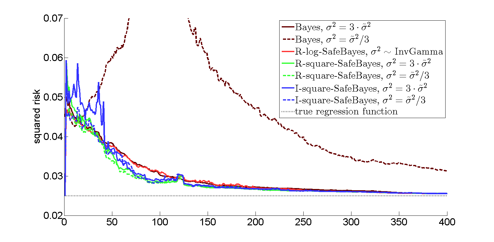
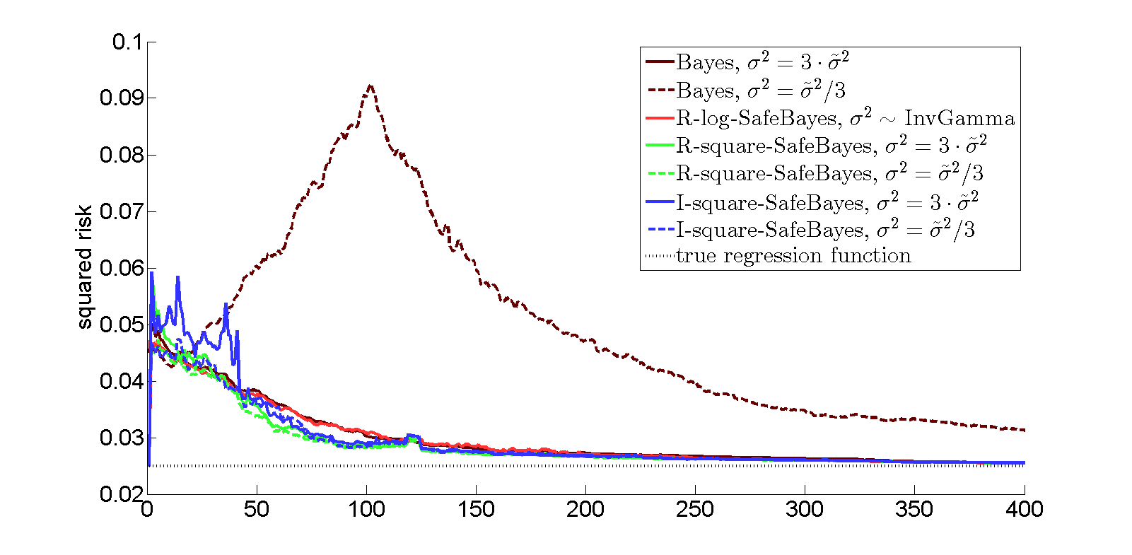
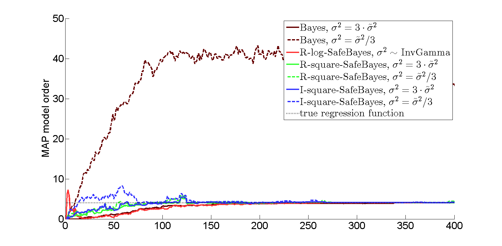
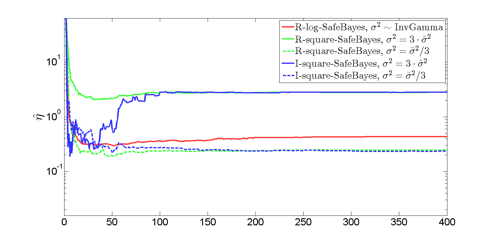
Figure 14: Bayesian Model Selection, fixed $\sigma^{2}$, for the model-wrong experiment of Figure 3 with $p_{\max}=50$. The second graph is a scaled version of the first. Since fixed $\sigma^{2}$ implies fixed overconfidence ratio, the overconfidence graph is not shown. For clarity in the $\eta$-graph we do not show standard deviations of the $\eta$’s.

A.1.2 Ridge Regression Experiments, Fixed $\sigma^{2}$

Again we only show results for the model-wrong experiment.

Note that here standard Bayes — as can be seen from plugging $\eta=1$ into (12) — does not depend on $\sigma^{2}$ and thus coincides in terms of square-risk behavior with standard Bayes in the variable $\sigma^{2}$ case as in Figure 7. Also (see below (12)) $I$-square-SafeBayes for fixed $\sigma^{2}$ does not itself depend on $\sigma^{2}$ and simply minimizes the cumulative sum of squared errors.

Just as for ridge regression with variable $\sigma^{2}$, one may equivalently interpret the $\eta$-generalized-posterior means $\bar{\beta}_{i,\eta}$ as the standard, nongeneralized Bayesian posterior means that one would get with a modified prior on $\beta$, proportional to the original prior raised to the power $\eta^{-1}$ (see above (31), Section 5.4). It may then once again seem reasonable to learn $\eta$ itself in a Bayesian- or likelihood-based way such as empirical Bayes. Indeed, this was suggested implicitly as early as 1999 by one of us (Grünwald, 1999). The procedure described in Section 3.4.3 (‘hierarchical loss’) of Bissiri et al. (2016) also arrives, via a different derivation, at a similar prescription for finding $\eta$ (we immediately add that the authors describe many ways for determining $\eta$, of which this is just one). Unfortunately, just as for the empirical Bayes learning of $\eta$ with varying $\sigma^{2}$, the figures below indicate that it does not perform well at all.

Conclusion

Standard Bayes again performs comparably badly in both experiments (note the difference in scale in the first graphs of Figure 14 and 15). $I$-square-SafeBayes behaves excellently in both experiments. But now in the ridge experiment $R$-square-SafeBayes becomes a highly problematic method for small samples, worse even than standard Bayes. The reason is its dependence on the specified $\sigma^{2}$ as can be clearly seen from (23). If $\sigma^{2}$ was set to be much larger than the actual average prediction error on the sample, then the third term in (23) dominates. This term decreases with $\eta$ and thus automatically pushes $\hat{\eta}$ ‘upward’ by an arbitrary amount. The term also decreases with $n$, so that the problem disappears at a large enough sample size. The problem did not occur in the model averaging experiment; we suspect that this is because in this experiment, there is substantial prior mass on a small model $p=4)$ containing the pseudo-truth, and for this submodel, the final term in (23) (which is approximately linear in $p$) is much smaller than for $p=50$ and does have not such a strong influence.

Figure 15: Bayesian Ridge Regression: same graphs as in Figure 7, for fixed $\sigma$ and the model-wrong experiment conditioned on $p:=p_{\max}=50$. Note the difference in scale for the risk in this figure and Figure 14.

A.2 Slightly Informative Prior

Again we only consider model-wrong experiments. Within each model, we now use the following prior parameters: $\bar{\beta}_{0}=\mathbf{0}$ and $\Sigma_{0}=10^{3}\mathbf{I}$ for the multivariate normal distribution on $\beta$; and $a_{0}=1$ and $b_{0}=\sigma^{*2}a_{0}$ (as before) for the inverse gamma distribution on $\sigma^{2}$ (where $\sigma^{*2}$ is the true variance of noise in our data, as defined in Section 5.1.2). We repeated the model-wrong experiment of Section 5.3 with $p_{\max}=50$ with this slightly informative prior and obtained similar results to those obtained using our original informative prior with $\Sigma_{0}=\mathbf{I}$: Bayes performs badly roughly between samples 90 and 130 and has some risk spikes before that so that its overall performance is comparable to before, while $R$-SafeBayes and $I$-SafeBayes both obtain good risks.

We also repeated the model-wrong experiment for ridge regression (Section 5.4). Here the effect of the new prior on Bayes’ performance is similar: the square-risk peaks at a larger value, but in a smaller range of sample sizes. However, the effect of changing the learning rate is different in this experiment than what we have seen before: here one can take $\eta$ very small and still get good results. So in a sense, the problematic behavior of Bayes has a trivial solution here: just pick a very small but fixed $\eta$. $R$-log-SafeBayes was too conservative in this, $I$-log-SafeBayes did fine. $R$-log-SafeBayes became competitive again however, if we used the discounting version described in Section B.1 below.

We omit the pictures corresponding to model selection/averaging (Section 5.3) as they show no surprises; but in Figure 16 we do repeat the pictures for ridge regression (Section 5.4), because they do give additional insight:

Figure 16: Top two graphs: square-risk for two different ridge experiments. In both experiments the slightly informative prior of Section A.2 is used. In the first experiment $p=50$; in the second $p=100$; otherwise the experiments are just as the ‘wrong model experiment’ of Section 5.4, Figure 7, but we also included performance of $I$-square-SafeBayes. Final graph shows self-confidence for the $p=100$ case for Bayes and SafeBayes, on a logarithmic scale because of the range of values involved.

Note that the phenomenon is now much more ‘temporary’. In the beginning, it seems that there is a sort of cancellation between the influence of the irrelevant variables and standard Bayes behaves fine. However, if we increase the number of irrelevant variables, the problem (while starting at a later sample) takes longer to recover from.

A.3 Prior as advised by Raftery et al.

In Raftery et al. (1997), some guidelines for choosing priors in regression models are given. Letting $\bar{\beta}_{0}$ denote the prior mean, one of their recommendations is that the prior densities for $\beta=\bar{\beta}_{0}$ and $\beta=\bar{\beta}_{0}+\mathbf{1}$ should differ by a factor of at most $\sqrt{10}$. The prior density on $\beta$ marginalized over $\sigma^{2}$ follows a multivariate t-distribution, and the factor in question varies with the dimensionality of $\beta$, so that models of larger order are given less informative priors. In our case, we find that the resulting prior is always less informative than our original prior, and for model $\mathcal{M}_{10}$ and above (i.e. $\beta$ of dimension 11 or larger), it becomes even less informative than the prior introduced in the previous section.

For the prior on $\sigma^{2}$, Raftery et al. advise that the density should vary by no more than a factor 10 in a region of $\sigma^{2}$ from some small value to the sample variance of $y$. For our choice of hyperparameters $a_{0}=1$, $b_{0}=1/40$, the mode of $\pi(\sigma^{2})$ is at $b_{0}/(a_{0}+1)=1/80$, and the density is within a factor 10 of this maximum in the approximate region $(0.0037,0.0941)$. For the correct model experiments, the actual variance of $Y$ is $0.065$; for the wrong model experiments, it is $0.045$ (with a larger variance for ‘good’ points and zero variance for ‘easy’ points). For both experiments, the factor-10 condition holds between $\textrm{Var}(Y)/12$ and $\textrm{Var}(Y)$. We conclude that this prior satisfies the guidelines in Raftery et al. quite well.

We will refer to the prior described above as Raftery’s prior (even though it is really a different prior for each model order). Using this prior, we found the following experimental results.

In the model-wrong experiment with model selection/averaging (Section 5.3) with our original prior replaced by Raftery’s prior, Bayes performs somewhat better than $R$-log-SafeBayes (except on very small sample sizes). However, $I$-log-SafeBayes performs as well as Bayes, and so does the $R$-log-SafeBayes variant that discounts half of the initial sample when choosing the learning rate (see Section B.1).

This might suggest that Raftery’s prior could be used to accomplish the same kind of safety against wrong models as SafeBayes provides, at least in a model selection context. To test this, another experiment was performed where the fraction of ‘easy’ points was increased to 75%. In this experiment, the misbehavior of Bayes seen in Section 5.3 returned worse than before, with risks a factor 20 larger than before, whereas the SafeBayes methods continued to work fine. This suggests that Raftery’s prior can not be relied on if the severeness of misspecification is unknown.

If Raftery’s prior is used for model selection with a correct model, Bayes and the SafeBayes variants perform well, and very similarly to each other.

For ridge regression, the results with Raftery’s prior for both the correct and the incorrect model experiment are very similar to those with the slightly informative prior, except that the peak in the risks is higher for all methods.

A.4 The $g$-prior

Another prior we experimented with was the $g$-prior, a popular choice in model selection contexts (Zellner, 1986, Liang et al., 2008). For all definitions we refer to the latter paper. In contrast to all other priors we considered, the $g$-prior depends on the design matrix ${\bf X}^{T}_{n}{\bf X}_{n}$, and hence can only be used in settings where this matrix, and hence the eventual sample size of interest $n$, is given once and for all. For this reason, we decided to depict in Figure 17, for each value of $n$, the risk obtained when predicting the $n$-th data point with the posterior calculated from the $g$-prior corresponding to the first $n$ covariates $(x_{1},\ldots,x_{n})$ and observed data $y^{n-1}$. This is subtly different from our previous graphs (e.g. Figure 3–6) that show how the risk evolves as $n$ increases in a single run of the experiment, averaged over 30 runs.

The graph is not shown starting at $n=0$, because of another difference between the $g$-prior and the priors we used in other experiments:

Because of the same design dependence, with the $g$-prior, the posterior on $\beta$ remains a degenerate distribution on an initial segment of outcomes. For example, with $\mathcal{M}_{p}$ for $p=50$, the matrix ${\bf X}_{n}^{T}{\bf X}_{n}$ is singular until at least 50 different design vectors have been observed. For our model-wrong experiment, this means that on average, about a 100 observations are required before the posterior becomes nondegenerate; this explains why Figure 17 starts at $n$ a little over a 100.

The experimental results clearly indicate that the $g$-prior does not deal with our data in a satisfactory way, regardless of the value of $g$. Of the values of $g$ we tried (up to $10^{4}$), $g\approx 100$ (shown in the graph) yielded the smallest squared risk around sample size $n=200$; for larger sample sizes, larger values of $g$ were better, but only slightly. Furthermore, (as in fact we expected by analogy to learning $\eta$ with Empirical Bayes), the value of $g$ found by Empirical Bayes is not optimal for dealing with our data and only makes things worse: larger values of $g$ (which put more weight on the data) would yield smaller risks.

Figure 17: Risk as a function of sample size (starting at the first sample size at which the $g$-prior is defined) for model averaging and selection based on the $g$-prior in the model-wrong experiment of Figure 3 both with $g=100$ and with $g$ chosen by Empirical Bayes at each sample size

Appendix B Experiments on Variations on the Method

Below we look at a number of other more or less promising alternative approaches to modifying standard Bayes.

B.1 An Idea to be Explored Further: Discounting Initial Observations

Just like standard Bayes, all our SafeBayesian methods are, at heart, prequential (Dawid, 1984). All prequential methods suffer to a greater or lesser extent from the start-up problem (van Erven et al., 2007, Wong and Clarke, 2004): sequential predictions based on a model $\mathcal{M}_{p}$ may perform very badly for the first few samples. While they quickly recover when the sample size gets large, the behavior on the first few samples may dominate their cumulative prediction error for a while, leading to suboptimal choices for moderate $n$. We can address this issue in several ways. A very simple method to ‘discount’ initial observations, apparently first used (implicitly) to modify standard Bayes factors by (Lempers, 1971, Chapter 6), is to only look at the cumulative sequential prediction error on the second half of the sample, so that the first half of the sample merely functions as a ‘warming-up’ sample (Catoni, 2012). Without claiming that this is the ‘right’ method to discount initial observations, we experimented with it to see whether it can further improve the performance of SafeBayes; for simplicity, we concentrated on $R$-log-SafeBayes.

We found that in most experiments, this new method for determining $\eta$ performed very similarly to the standard method based on the whole sample, sometimes slightly better and sometimes slightly worse, making it hard to say whether the new method is an improvement or not. Still, there are two experiments in which the new method performed substantially better, namely the experiments with less informative priors of Section A.2 and A.3. Thus we cannot just dismiss the idea of fitting $\eta$ based on only part of the data or more generally, discounting initial observations, and it would be interesting to explore this further in future work: of course taking half of the data is rather arbitrary, and better choices may be possible. In particular, we may try a variation of switching between $\eta$’s analogously to the switch distribution (van Erven et al., 2007) to counter the startup problem.

B.2 Other Methods for Model Selection: AIC, BIC, (generalized) Cross-Validation

We tested the performance of several classic model selection methods on the same data and models as in our main model selection/averaging experiment, Section 5.3. We associated with each model $\mathcal{M}_{p}$ its standard (i.e. $\eta=1$) Bayes predictive distribution under the prior described in Section 5.1 (these generally perform better than the maximum likelihood distributions based on $\mathcal{M}_{p}$ whose use is more standard here). We then ran leave-one-out cross-validation, 10-fold cross-validation and GCV based on the predictions (posterior means/MAPs $\bar{\beta}_{i,\eta}$) made by these predictive distributions.

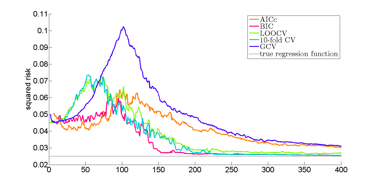
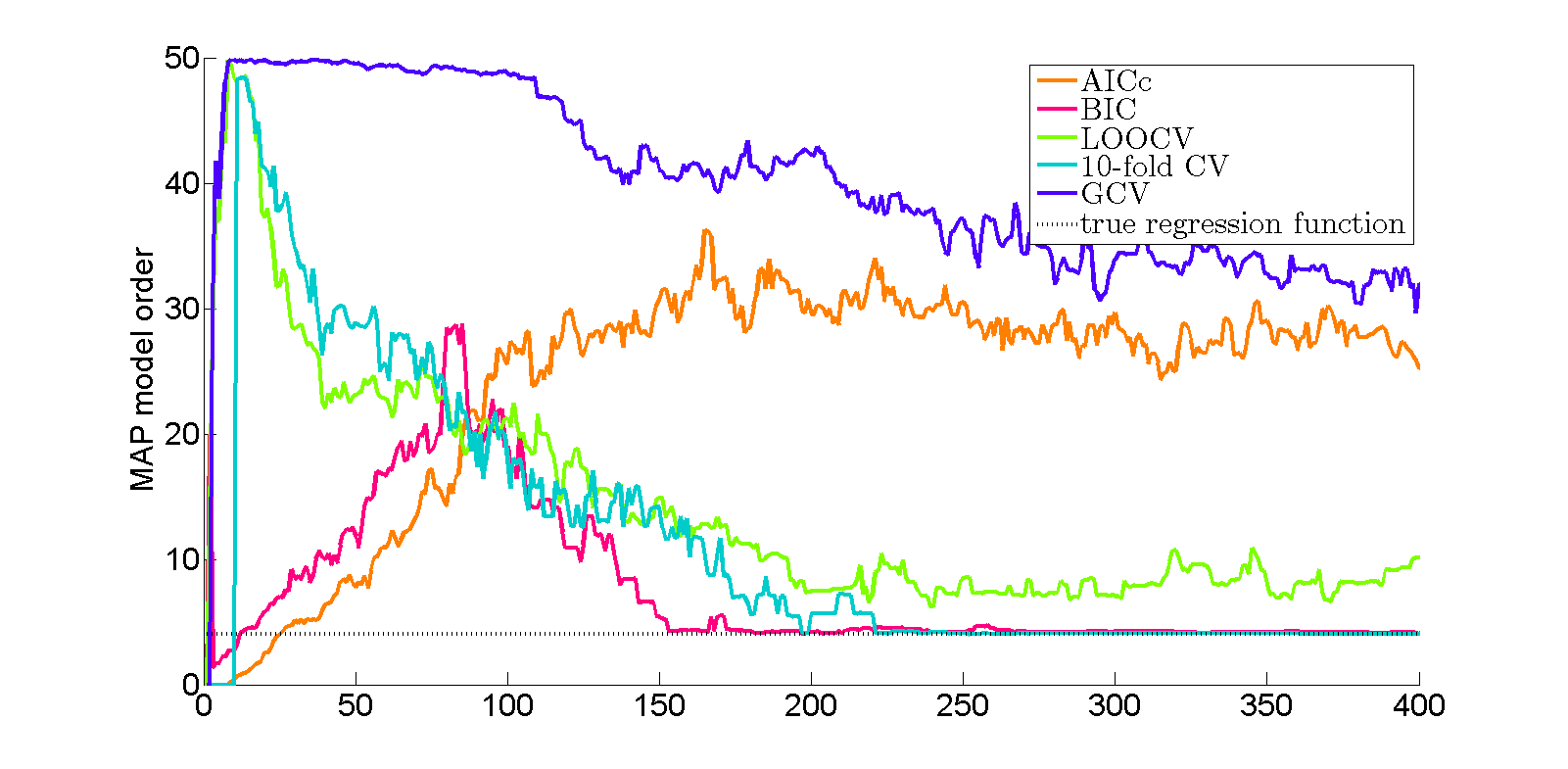
Figure 18: Squared risk and selected model order for five different model selection methods. The risks in this graph are risks of single models selected by each method (similar to the MAP risks shown for Bayes and SafeBayes).

We also compared the models via AIC and BIC, where for AIC we used the small-sample correction of Hurvich and Tsai (1989).

We see that AIC and generalized cross-validation have risks and selected model orders similar to those of standard Bayes, though they do not recover as well as Bayes when the sample size increases. Of the other three methods, BIC and 10-fold cross-validation find the optimal model and have smaller risks towards the end than leave-one-out cross-validation, which continues to select larger-than-optimal models with substantial probability. Note that none of the methods can compete with SafeBayes on sample sizes below 150: SafeBayes’s risk goes down immediately after the start of the experiment while for all the other methods it goes up first. Also, SafeBayes finds the optimal model quickly without first trying much larger models.

B.3 Other Methods for Learning $\eta$: Cross-Validation on Log-Loss and on Squared Loss

As indicated in the introduction and Section 4.2, finding $\hat{\eta}$ by $I$-square-SafeBayes is somewhat similar to finding $\hat{\eta}$ by leave-one-out cross-validation with the squared-error loss, the difference being that $I$-square-SafeBayes finds the optimal $\eta$ for predicting each point based on past data data points rather than the optimal $\eta$ for predicting each point based on all other data points. Since the leave-one-out method is often employed in ridge regression, it seemed of interest to try out here as well. Figure 19 shows that LOO-cross validation indeed performs very similarly to $R$-log and $I$-square SafeBayes in terms of square-risk, but is consistently a bit worse in terms of self-confidence; we do not have a clear explanation for this phenomenon.

Perhaps more interestingly, in Figure 20 we show what happens if we use LOO-cross validation based on the log-loss of the Bayes predictive distribution, which may seem a reasonable procedure from a ‘likelihoodist’ perspective. Here we see dismal behavior, the reason being the hypercompression phenomenon of Section 6.3: cross-validation will select a model that, at the given sample size, has small log-risk, but because of hypercompression this model can sometimes perform very badly in terms of all the associated prediction tasks such as square-risk and reliability.

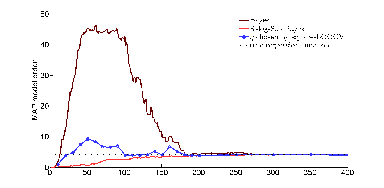
Figure 19: Analogue of Figure 3 for determining $\eta$ by leave-one-out cross-validation with square-loss with the wrong-model experiment, $p_{\max}=50$.

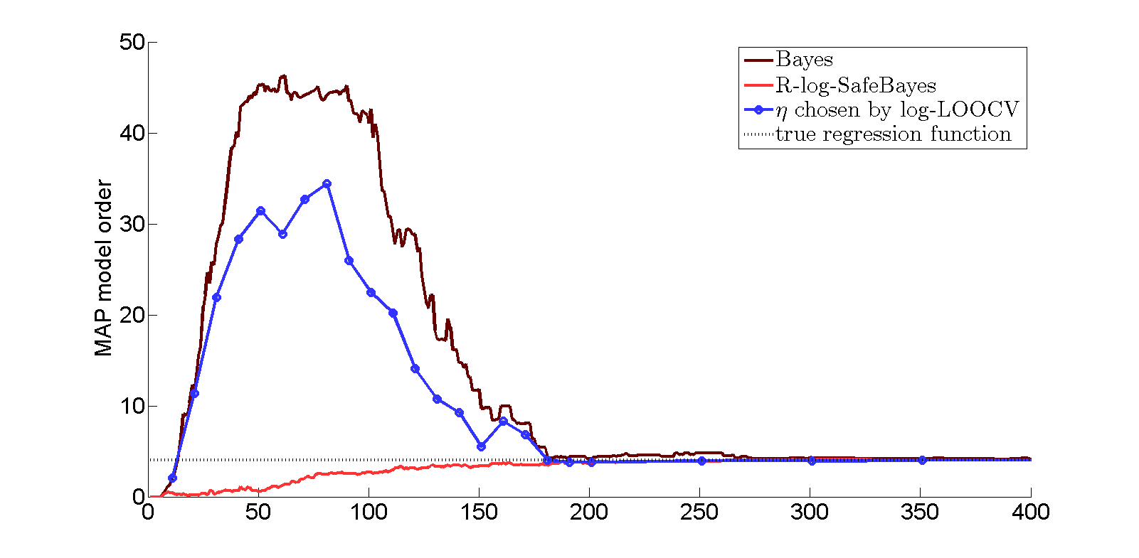
Figure 20: Analogue of Figure 3 for determining $\eta$ by leave-one-out cross-validation with log-loss.

Appendix C Experiments on Variations of the Truth

Other Distributions of Covariates

In all experiments described in Section 5 and the previous appendices, the covariates $(X_{i1},X_{i2},\ldots)$ where sampled independently from a $0$-mean multivariate Gaussian. We repeated most of our experiments with $X_{i1},X_{i2},\ldots$ that were sampled independently uniformly from $[-1,1]$, and, as already indicated in the introduction, with polynomials, $X_{ij}=S_{i}^{j}$ for $S_{i}\in[-1,1]$ uniform. This did not change the results in any substantial way, so we do not report on it further.

Fewer Easy and ‘Less-Easy’ Points

If the fraction of ‘easy’ points is reduced, one would expect the performance of standard Bayes to improve. This is confirmed by an experiment where each data point had a probability of only $1/4$ to be $(0,0)$. Here Bayes still has some trouble finding the optimal model, but the square-risk, MAP model order, and time taken to recover are all much reduced compared to the original experiment in Section 5.3 where half the data points were ‘easy’. SafeBayes on the other hand showed the same good performance as before.

Two points that might be raised against the use of ‘easy’ points in our simulations are that they are unlikely to occur in practice, and that if they were to occur, they would be easily detected and dealt with another way. To address this line of argument to some extent, another experiment was performed with a smaller contrast between ‘easy’ and ‘hard’ points. Rather than being identically $(0,0)$, the ‘easy’ points were random but with smaller variance than the ‘hard’ points. To be precise, the covariates and noise were both a factor 5 smaller (so that their variances were 25 times smaller). In this experiment, the same phenomena as in Section 5.3 occurred, albeit again on a smaller scale (though larger than in the previous, $1/4$-easy experiment).

Different Optimal Regression Functions

We experimented with a number of variations of the wrong-model experiment of Section 5.3, by changing the underlying ‘true’ distribution $P^{*}$. In each variation, we still tossed, at each $i$, an independent biased coin to determine whether $i$ would be ‘easy’ (still probability $1/2$) or ‘regular’ (probability $1/2$), but in each case we changed the definition of either the ‘easy’ or the ‘regular’ instances or both. In all experiments, for the ‘regular’ instances, only $P^{*}(Y_{i}\mid X_{i})$ was changed; the marginal distribution of the $X_{i}$ was still multivariate normal as before. Here is a list of things we tried:

1. For regular instances, set $P^{*}(Y_{i}\mid X_{i})$ so that $Y_{i}=0+\epsilon_{i}$ instead of (27), with $\epsilon_{i}$ i.i.d. normal as before; easy instances were still set to $({\bf 0},0)$.

2. For regular instances, (27) was replaced by $Y_{i}=X_{i1}+X_{i2}+X_{i3}+X_{i4}+\epsilon_{i}$, so the optimal coefficients $\tilde{\beta}_{1}\ldots\tilde{\beta}_{4}$ are ten times as large as in the original experiment; easy instances were still set to $({\bf 0},0)$.

3. For regular instances, (27) was replaced by $Y_{i}=.1\cdot(X_{i1}+\ldots+X_{i4})-.04+\epsilon_{i}$ (so the intercept is not $0$), and the easy instances were set to $(X_{i},Y_{i})$ = $({\bf.2},.04)$, where ${\bf.2}$ represents the $K$-dimensional vector $(.2,\ldots,.2)$. Note that the easy points are on the optimal regression function.

4. For regular instances, (27) was replaced by $Y_{i}=.1\cdot(X_{i1}+\ldots+X_{i4})+.5+\epsilon_{i}$ so the intercept was again not $0$; the easy instances were set to $({\bf 0},.5)$.

We explain each in turn. For the first experiment, all the results were comparable to the results of Experiment 1 in Section 5, so we do not list them. For the second experiment, the risks obtained by standard Bayes and SafeBayes were similar to each other. The model order behaviors were similar to what they were before (with standard Bayes selecting large model orders initially), but all methods recovered much more quickly, converging on the optimal model shortly after $n=50$; presumably this could happen because now the optimal coefficients were substantially larger than the standard deviation in the data.

The third experiment was included to see whether there would be an effect if the ‘easy’ points would be placed at an arbitrary point rather than the special, fully symmetric $({\bf 0},0)$. We added the intercept $-0.04$ so as to make sure that, for the data we actually observe, $\mathbf{E}_{X,Y\sim P^{*}}[Y_{i}]=(1/2).04-(1//2).04=0$; thus the $Y$-values will appear centered around $0$, which is standard both in frequentist and Bayesian approaches to regression (for example, both Raftery et al. (1997) and Hastie et al. (2001) preprocess the data so that $\sum_{i=1}^{n}Y_{i}=0$). Again, we discerned no difference in the results so did not include any further details.

Finally, the fourth experiment was included just to see what happens if, contrary to standard methodology, we apply the method to $Y_{i}$ that are not (even approximately) centered. In this experiment, standard Bayes did not converge to the optimal model until after $n=150$ as in the experiment of Section 5.3, but its risk and selected model orders were both smaller. The versions of SafeBayes worked well as before.

Appendix D More on Mix Loss

D.1 Implementing SafeBayes

To implement the Safe Bayesian algorithm (page 1), generalized posteriors must be computed for different values of $\eta$, and the randomized loss (18) must be computed for each sample size. For linear models with conjugate priors as considered in our experiments, all required quantities can be computed analytically. We have already seen how to do this for models ${\cal M}_{p}$ with fixed dimension $p$. For unions of such models, it turns out that the mix-loss is a helpful tool.

Role of mix loss in generalized posterior over models

The generalized posterior across a discrete set of models is given by (7), which, writing $\tau=(\beta,\sigma^{2})$, is, via (10) and (3.1), equivalent to

$$\pi(p\mid z^{n},\eta) =\int_{\Theta_{p}}\pi(p,\tau\mid z^{n},\eta)\,d\tau$$

$$\propto\int(\/{f}(y^{n}\mid x^{n},\tau,p)\/)^{\eta}\pi(\tau\mid p)\,d\tau\,\pi(p).$$ (46)

Here $\propto$ means ‘proportional to’ when $p$ is varied and $z^{n}$ and $\eta$ are fixed. In practice we prefer to calculate this quantity incrementally: the posterior for $z^{n+1}$ with prior $\Pi$ is equal to the posterior for a single data point $z_{n+1}$ when the posterior for $z^{n}$ is used as prior (in this sense the generalized posterior behaves like the standard posterior): using this to further rewrite the second line of (D.1) gives

$$\pi(p\mid z^{n},\eta) \propto\int(\/{f}(y^{n}\mid x^{n},\tau,p)\/)^{\eta}\pi(\tau\mid p)\,d\tau\,\pi(p)$$

$$=\int(\/{f}(y_{n}\mid x_{n},\tau,p)\/)^{\eta}\cdot(\/{f}(y^{n-1}\mid x^{n-1},\tau,p)\/)^{\eta}\pi(\tau\mid p)\,d\tau\,\pi(p)$$

$$=\int(\/{f}(y_{n}\mid x_{n},\tau,p)\/)^{\eta}\cdot\left(\pi(\tau\mid z^{n-1},p,\eta)\cdot\int(\/{f}(y^{n-1}\mid x^{n-1},\tau^{\prime})^{\eta}\pi(\tau^{\prime}\mid p)d\tau^{\prime}\,\right)\,d\tau\,\pi(p)$$

$$\propto\int(\/{f}(y_{n}\mid x_{n},\tau,p)\/)^{\eta}\cdot\pi(\tau\mid z^{n-1},p,\eta)\,d\tau\cdot\pi(p\mid z^{n-1},\eta),$$

where in the third inequality we used the definition of the generalized posterior and in the last we used (D.1).

The integral appearing in both the cumulative and the step-wise expression equals the expectation in (40) from the $\eta$-flattened $\eta$-generalized Bayesian predictive density for $n$ and $1$ outcome respectively; $-\log[(\cdot)^{1/\eta}]$ of this quantity is the mix loss of model $p$. We will now derive formulas for this quantity.

Model with fixed variance

Use the notation of Section 3.1. Write $\sigma^{2}_{\text{mix}}=\sigma^{2}(1/\eta+x_{n+1}\Sigma_{n}x_{n+1}^{T})$. Then the mix loss for predicting one new data point $y_{n+1}$ is

$$-\log\bar{{f}}(y_{n+1}\mid x_{n+1},z^{n},\langle\eta\rangle;\eta)\\ =\frac{1}{\eta}\left[\frac{1}{2}(\eta-1)\log(2\pi\sigma^{2})+\frac{1}{2}\log\eta+\frac{1}{2}\log(2\pi\sigma^{2}_{\text{mix}})+\frac{1}{2\sigma^{2}_{\text{mix}}}(y_{n+1}-x_{n+1}\beta_{n})^{2}\right]$$

Model with conjugate prior on variance

Using the notation of Section 3.1, the mix loss is given by

$$-\log\bar{{f}}(y_{n+1}\mid x_{n+1},z^{n},\langle\eta\rangle;\eta)=\frac{1}{\eta}\biggl{[}\frac{1}{2}\eta\log\pi+\frac{1}{2}\log(1+\eta x_{n+1}\Sigma_{n}x_{n+1}^{T})\\ +a_{n+1}\log(2b_{n}+\frac{(y_{n+1}-x_{n+1}\beta_{n})^{2}}{1/\eta+x_{n+1}\Sigma_{n}x_{n+1}^{T}})-a_{n}\log 2b_{n}-\log\frac{\Gamma(a_{n+1})}{\Gamma(a_{n})}\biggr{]},$$

D.2 Belief in Concentration (proof of Theorem 1)

For simplicity, we only give the proof for the unconditional case, in which the $\theta$ represent distributions $P_{\theta}$ on $z\in\mathcal{Z}$; extension to the conditional case is straightforward. For $0<\eta<1$, let $d_{\eta}(\theta^{*}\|\theta)$ denote the Rènyi divergence of order $1-\eta$ (van Erven and Harremoës, 2014), i.e. $d_{\eta}(\theta^{*}\|\theta)=-\frac{1}{\eta}\log\mathbf{E}_{Z\sim\theta^{*}}\left(\frac{{f}_{\theta}(Z)}{{f}_{\theta^{*}}(Z)}\right)^{\eta}$. We first state a lemma, proved further below. In the lemma, as in the remainder of the proof, $(\theta^{*},Z^{n})$ is the random variable distributed according to the Bayesian distribution $\Pi$.

Lemma 1

Let $\Theta$, $\Pi$ and $\pi$ be as in the statement of Theorem 1. For every $1/2\leq\eta<1$, $\epsilon>0$, let $\bar{\Theta}_{\eta,\epsilon}:=\{\theta\in\Theta:d_{\eta}(\theta^{*}\|\theta)>\epsilon\}$. For every $b>0$ and every sample size $n$ and setting $\epsilon:=(b\log n)/(n\eta)$ and $c_{\eta}=(1-\eta)/(1+\eta(1-\eta))$, we have:

$$\Pi\left(\ \Pi(\bar{\Theta}_{\eta,\epsilon}\mid Z^{n})\geq n^{-bc_{\eta}}\ \right)\leq 2\left(\sum_{\theta\in\Theta}\pi(\theta)^{\eta}\right)\cdot n^{-bc_{\eta}}.$$

In particular, if $\pi$ is summable for some $\eta<1$, then using $b=1/c_{\eta}$, we get that the Bayesian probability that the posterior probability of the set of $\theta$ farther than $b(\log n)/n$ from $\theta^{*}$ exceeds $1/n$, is $O(1/n)$.

We proceed to prove Theorem 1 using this lemma. By the information inequality, we have for every probability density ${f}\neq{f}_{\theta^{*}}$ that

$$D(\theta^{*}\|\theta)=\mathbf{E}_{Z_{n}\sim P_{\theta^{*}}}[-\log{f}_{\theta}(Z_{n})+\log{f}_{\theta^{*}}(Z_{n})]\geq\mathbf{E}_{Z_{n}\sim P_{\theta^{*}}}[-\log{f}_{\theta}(Z_{n})+\log{f}(Z)].$$

In particular this holds with ${f}=\bar{{f}}\mid Z^{n}$, the Bayes predictive distribution based on the sample seen so far. It then follows from (6.4) that

$$\bar{\delta}_{n}\leq\mathbf{E}_{\theta\sim\Pi\mid Z^{n}}[D(\theta^{*}\|\theta)]$$ (47)

Since $\pi^{\eta}$ is decreasing in $\eta$, we may without loss of generality assume that the $\eta$ mentioned in the theorem statement is at least $1/2$. Now note (van Erven and Harremoës, 2014, Theorem 16) that for every $1/2<\eta<1$, $d_{1/2}(\theta^{*}\|\theta)\leq(\eta/(1-\eta))\cdot d_{\eta}(\theta^{*}\|\theta)$. We also know from (Yang and Barron, 1999, Lemma 4) that the KL divergence $D(\theta^{*}\|\theta)$ satisfies $D(\theta^{*}\|\theta)\leq(2+\log v)d_{1/2}(\theta^{*}\|\theta)$. Since trivially $d_{\eta}(\theta^{*}\|\theta)\leq\log v$, we have, with $C=\frac{\eta}{1-\eta}\cdot(2+2\log v)$, for every $\epsilon>0$, using (47),

$$\bar{\delta}_{n}\leq C\cdot\mathbf{E}_{\theta\sim\Pi\mid Z^{n}}[d_{\eta}(\theta^{*}\|\theta)]\\ \leq C\Pi\left(d_{\eta}>\epsilon\mid Z^{n}\right)\log v+C\left(1-\Pi\left(d_{\eta}>\epsilon\mid Z^{n}\right)\right)\epsilon\leq C\left(\Pi\left(d_{\eta}>\epsilon\mid Z^{n}\right)\log v+\epsilon\right),$$ (48)

so that $\Pi\left(d_{\eta}>\epsilon\mid Z^{n}\right)\geq(C^{-1}\bar{\delta}_{n}-\epsilon)/(\log v)$ and by Lemma 1, we have for $\epsilon=b(\log n)/(n\eta)$ as in the lemma, that

$$\Pi\left(\ \frac{C^{-1}\bar{\delta}_{n}-\epsilon}{\log v}\geq n^{-bc_{\eta}}\ \right)\leq 2\left(\sum_{\theta\in\Theta}\pi(\theta)^{\eta}\right)\cdot n^{-bc_{\eta}}.$$

Rewriting this expression, plugging in the value of $\epsilon$ and using $\eta\geq 1/2$, gives

$$\Pi\left(\ \bar{\delta}_{n}\geq C\left((\log v)n^{-bc_{\eta}}+\frac{2b(\log n)}{n}\right)\ \right)\leq 2\left(\sum_{\theta\in\Theta}\pi(\theta)^{\eta}\right)\cdot n^{-bc_{\eta}}.$$ (49)

The first part of the result follows by setting $b=a/c_{\eta}$. For the second result, note that the first result implies (take $a=2$), by the union bound over sample sizes $1,\ldots,n$, that the Bayesian probability that $\mathbf{E}_{Z^{n}\sim\theta^{*}}[\Delta_{n}]$ exceeds $C_{0}\sum_{i=1}^{n}(\log i)/i\asymp(\log n)^{2}$ is $O(1/n)$. Thus there exists $C^{\prime},C^{\prime}_{0}$ such that the Bayesian probability that $\mathbf{E}_{Z^{n}\sim\theta^{*}}[\Delta_{n}]$ exceeds $C^{\prime}_{0}(\log n)^{2}$ is bounded by $C^{\prime}/n$. Thus for the probability in (39) we have

$$\Pi\left(\ {\Delta}_{n}\geq C_{2}\cdot n^{a^{\prime}}\ \right)= \Pi\left(\ {\Delta}_{n}\geq C_{2}\cdot n^{a^{\prime}},\mathbf{E}_{Z^{n}\sim\theta^{*}}[\Delta_{n}]\geq C^{\prime}_{0}(\log n)^{2}\ \right)+$$

$$\Pi\left(\ {\Delta}_{n}\geq C_{2}\cdot n^{a^{\prime}},\mathbf{E}_{Z^{n}\sim\theta^{*}}[\Delta_{n}]<C^{\prime}_{0}(\log n)^{2}\ \right)$$

$$\leq \Pi\left(\ \mathbf{E}_{Z^{n}\sim\theta^{*}}[\Delta_{n}]\geq C^{\prime}_{0}(\log n)^{2}\ \right)+$$

$$\Pi\left(\ {\Delta}_{n}\geq C_{2}\cdot n^{a^{\prime}},\mathbf{E}_{Z^{n}\sim\theta^{*}}[\Delta_{n}]<C^{\prime}_{0}(\log n)^{2}\ \right)$$

$$\leq \frac{C^{\prime}}{n}+\frac{C^{\prime}_{0}(\log n)^{2}}{C_{2}n^{a^{\prime}}},$$

where in the final step we used Markov’s inequality. The second result follows.

Proof of Lemma 1

Fix $A>0$ and $\gamma>0$. We have

$$\Pi\left(\Pi(\bar{\Theta}_{\eta,\epsilon}\mid Z^{n})\geq A\right)=\Pi\left(\frac{\sum_{\theta\in\bar{\Theta}_{\eta,\epsilon}}\pi(\theta)\cdot{f}_{\theta}(Z^{n})}{\sum_{\theta\in\Theta}\pi(\theta)\cdot{f}_{\theta}(Z^{n})}\geq A\right)=\\ \Pi\left(\frac{\sum_{\theta\in\bar{\Theta}_{\eta,\epsilon}}\pi(\theta)\cdot{f}_{\theta}(Z^{n})}{{f}_{\theta^{*}}(Z^{n})}\cdot\frac{{f}_{\theta^{*}}(Z^{n})}{\sum_{\theta\in\Theta}\pi(\theta)\cdot{f}_{\theta}(Z^{n})}\geq A\right)\leq\\ \Pi\left(\frac{\sum_{\theta\in\bar{\Theta}_{\eta,\epsilon}}\pi(\theta)\cdot{f}_{\theta}(Z^{n})}{{f}_{\theta^{*}}(Z^{n})}\geq A^{1+\gamma}\right)+\Pi\left(\frac{{f}_{\theta^{*}}(Z^{n})}{\sum_{\theta\in\Theta}\pi(\theta)\cdot{f}_{\theta}(Z^{n})}\geq A^{-\gamma}\right),$$ (50)

where we used the union bound. The first term is equal to, and can be further bounded as

$$= \Pi\left(\frac{\left(\sum_{\theta\in\bar{\Theta}_{\eta,\epsilon}}\pi(\theta)\cdot{f}_{\theta}(Z^{n})\right)^{\eta}}{({f}_{\theta^{*}}(Z^{n}))^{\eta}}\geq A^{\eta(1+\gamma)}\right)\leq\Pi\left(\frac{\sum_{\theta\in\bar{\Theta}_{\eta,\epsilon}}\pi(\theta)^{\eta}\cdot({f}_{\theta}(Z^{n}))^{\eta}}{({f}_{\theta^{*}}(Z^{n}))^{\eta}}\geq A^{\eta(1+\gamma)}\right)$$

$$= \sum_{\theta^{*}}\pi(\theta^{*})P_{\theta^{*}}\left(\frac{\sum_{\theta\in\bar{\Theta}_{\eta,\epsilon}}\pi(\theta)^{\eta}\cdot({f}_{\theta}(Z^{n}))^{\eta}}{({f}_{\theta^{*}}(Z^{n}))^{\eta}}\geq A^{\eta(1+\gamma)}\right)$$

$$\leq \sum_{\theta^{*}\in\Theta}\pi(\theta^{*})\mathbf{E}_{Z^{n}\sim P_{\theta^{*}}}\left[\frac{\sum_{\theta\in\bar{\Theta}_{\eta,\epsilon}}\pi(\theta)^{\eta}\cdot({f}_{\theta}(Z^{n}))^{\eta}}{({f}_{\theta^{*}}(Z^{n}))^{\eta}}\right]\cdot A^{-\eta(1+\gamma)}$$

$$= \sum_{\theta^{*}\in\Theta}\pi(\theta^{*})\sum_{\theta\in\bar{\Theta}_{\eta,\epsilon}}\pi(\theta)^{\eta}\cdot\left(\mathbf{E}_{Z\sim P_{\theta^{*}}}\left[\frac{({f}_{\theta}(Z))^{\eta}}{({f}_{\theta^{*}}(Z))^{\eta}}\right]\right)^{n}\cdot A^{-\eta(1+\gamma)}$$

$$\leq \left(\sum_{\theta\in\bar{\Theta}_{\eta,\epsilon}}\pi(\theta)^{\eta}\right)e^{-n\eta\epsilon}\cdot A^{-\eta(1+\gamma)}.$$

where the first inequality follows by differentiation to $\eta$ (or equivalently, by monotonicity of $\ell^{p}$-norms), the second is Markov’s, and the third is the definition of Rènyi divergence.

The second term in (50) can be bounded as

$$\leq \Pi\left(\frac{{f}_{\theta^{*}}(Z^{n})}{\pi(\theta^{*})\cdot{f}_{\theta^{*}}(Z^{n})}\geq A^{-\gamma}\right)=\Pi(\pi(\theta^{*})^{-1+\eta}\geq A^{-(1-\eta)\gamma})\leq\mathbf{E}_{\theta^{*}\sim\Pi}[\pi(\theta^{*})^{-1+\eta}]A^{\gamma(1-\eta)}$$

$$=\sum_{\theta^{*}}\pi(\theta^{*})^{\eta}A^{\gamma(1-\eta)}.$$

Combining the upper bounds on the two terms on the right in (50), we get:

$$\Pi\left(\Pi(\bar{\Theta}_{\eta,\epsilon}\mid Z^{n})\geq A\right)\leq\left(\sum_{\theta\in\bar{\Theta}_{\eta,\epsilon}}\pi(\theta)^{\eta}\right)\left(e^{-n\eta\epsilon}\cdot A^{-\eta(1+\gamma)}+A^{\gamma(1-\eta)}\right).$$

Now we plug in the chosen value of $\epsilon=(b\log n)/(n\eta)$ and we set $A=n^{-b/(\gamma+\eta)}$. With these values the second factor on the right becomes

$$e^{-n\eta\epsilon}\cdot A^{-\eta(1+\gamma)}+A^{\gamma(1-\eta)}=n^{-b}n^{b(\eta(1+\gamma))/(\gamma+\eta)}+n^{-b\gamma(1-\eta)/(\gamma+\eta)}=2n^{-b\cdot\gamma\cdot\frac{1-\eta}{\gamma+\eta}}.$$

Since this holds for al $\gamma>0$, it also holds for $\gamma=1/(1-\eta)$, and the result follows.

References

- Audibert (2004) J. Y. Audibert. PAC-Bayesian statistical learning theory. PhD thesis, Université Paris VI, 2004.
- Audibert (2007) J. Y. Audibert. Progressive mixture rules are deviation suboptimal. In NIPS, 2007.
- Barron (1987) A. R. Barron. Are Bayes rules consistent in information? In Open Problems in Communication and Computation, pages 85–91. Springer, 1987.
- Barron (1998) A. R. Barron. Information-theoretic characterization of Bayes performance and the choice of priors in parametric and nonparametric problems. In J. M. Bernardo, J. O. Berger, A. P. Dawid, and A. F. M. Smith, editors, Bayesian Statistics, volume 6, pages 27–52. Oxford University Press, Oxford, 1998.
- Barron and Cover (1991) A. R. Barron and T. M. Cover. Minimum complexity density estimation. IEEE Transactions on Information Theory, 37(4):1034–1054, 1991.
- Barron and Hengartner (1998) A. R. Barron and N. Hengartner. Information theory and superefficiency. Annals of Statistics, 26(5):1800–1825, 1998.
- Barron et al. (1998) A. R. Barron, J. Rissanen, and B. Yu. The minimum description length principle in coding and modeling. IEEE Transactions on Information Theory, 44(6):2743–2760, 1998. Special Commemorative Issue: Information Theory: 1948-1998.
- Barron et al. (1999) Andrew R. Barron, Mark J. Schervish, and Larry Wasserman. The consistency of posterior distributions in nonparametric problems. The Annals of Statistics, 27(2):536–561, 1999.
- Berk (1966) Robert Berk. Limiting behavior of posterior distributions when the model is incorrect. Annals of Mathematical Statistics, 37:51–58, 1966.
- Besag (1975) Julian Besag. Statistical analysis of non-lattice data. The statistician, pages 179–195, 1975.
- Bissiri et al. (2016) Pier Giovanni Bissiri, C. Holmes, and Stephen G. Walker. A general framework for updating belief distributions. Journal of the Royal Statistical Society: Series B (Statistical Methodology), 78(5):1103–1130, 2016.
- Box (1979) G. E. P. Box. Robustness in the strategy of scientific model building. In R. L. Launer and G. N. Wilkinson, editors, Robustness in Statistics, New York, 1979. Academic Press.
- Box (1980) George E. P. Box. Sampling and Bayes’ inference in scientific modelling and robustness. Journal of the Royal Statistical Society. Series A (General), pages 383–430, 1980.
- Breiman (2001) L. Breiman. Statistical modeling: The two cultures (with discussion). Statistical Science, 16(3):199 –215, 2001.
- Catoni (1997) O. Catoni. A mixture approach to universal model selection. Preprint LMENS-97-30, 1997. Available from http://www.math.ens.fr/edition/publis/Index.97.html.
- Catoni (2007) O. Catoni. PAC-Bayesian Supervised Classification. Lecture Notes-Monograph Series. IMS, 2007.
- Catoni (2012) O. Catoni. Discussion on the paper ‘Catching up Faster by Switching Sooner’ by Van Erven, Grünwald and De Rooij. Journal of the Royal Statistical Society: Series B (Statistical Methodology), 74(3):399–400, 2012.
- Cesa-Bianchi and Lugosi (2006) N. Cesa-Bianchi and G. Lugosi. Prediction, Learning, and Games. Cambridge University Press, Cambridge, UK, 2006.
- Csiszár and Shields (2000) I. Csiszár and P. Shields. The consistency of the BIC Markov order estimator. Annals of Statistics, 28:1601–1619, 2000.
- Cuong et al. (2013) Nguyen Viet Cuong, Wee Sun Lee, Nan Ye, Kian Ming A. Chai, and Hai Leong Chieu. Active learning for probabilistic hypotheses using the maximum Gibbs error criterion. In Advances in Neural Information Processing Systems 26, 2013.
- Dalalyan and Tsybakov (2012) Arnak S. Dalalyan and Alexandre B. Tsybakov. Mirror averaging with sparsity priors. Bernoulli, 18(3):914–944, 2012.
- Dawid (1982) A. P. Dawid. The well-calibrated Bayesian. Journal of the American Statistical Association, 77:605–611, 1982. Discussion: pages 611–613.
- Dawid (1984) A. P. Dawid. Present position and potential developments: Some personal views, statistical theory, the prequential approach. Journal of the Royal Statistical Society, Series A, 147(2):278–292, 1984.
- Dawid (2004) A. P. Dawid. Probability, causality and the empirical world: A Bayes–de Finetti–Popper–Borel synthesis. Statistical Science, 19:44–57, 2004.
- De Blasi and Walker (2013) Pierpaolo De Blasi and Stephen G. Walker. Bayesian asymptotics with misspecified models. Statistica Sinica, 23:169–187, 2013.
- de Rooij et al. (2014) S. de Rooij, T. van Erven, P. Grünwald, and W. Koolen. Follow the leader if you can, Hedge if you must. Journal of Machine Learning Research, 2014.
- Doob (1949) J. L. Doob. Application of the theory of martingales. In Le Calcul de Probabilités et ses Applications. Colloques Internationaux du Centre National de la Recherche Scientifique, pages 23–27, Paris, 1949.
- Doucet and Shephard (2012) Arnaud Doucet and Neil Shephard. Robust inference on parameters via particle filters and sandwich covariance matrices. Technical Report 606, University of Oxford, Department of Economics, 2012.
- Dümbgen et al. (2011) Lutz Dümbgen, Richard Samworth, and Dominic Schuhmacher. Approximation by log-concave distributions, with applications to regression. The Annals of Statistics, 39(2):702–730, 2011.
- Dunson and Taylor (2005) David B. Dunson and Jack A. Taylor. Approximate Bayesian inference for quantiles. Nonparametric Statistics, 17(3):385–400, 2005.
- van Erven et al. (2011) T. van Erven, P. Grünwald, W. Koolen, and S. de Rooij. Adaptive hedge. In Advances in Neural Information Processing Systems 24 (NIPS-11), 2011.
- van Erven and Harremoës (2014) Tim van Erven and Peter Harremoës. Rényi divergence and Kullback-Leibler divergence. IEEE Transactions on Information Theory, 60(7):3797–3820, 2014.
- Freund et al. (2004) Y. Freund, Y. Mansour, and R. E. Schapire. Generalization bounds for averaged classifiers (how to be a Bayesian without believing). Annals of Statistics, 32(4):1698–1722, 2004.
- Gelman (2004) A. Gelman. Bayes and Popper. Entry in A. Gelman’s blog on Statistical Modeling, Causal Inference, and Social Science, October 2004.
- Gelman and Shalizi (2012) A. Gelman and C. Shalizi. Philosophy and the practice of Bayesian statistics. British Journal of Mathematical and Statistical Psychology, 2012.
- Gelman et al. (2013) A. Gelman, J. B. Carlin, H. S. Stern, D. B. Dunson, A. Vehtari, and D. B. Rubin. Bayesian Data Analysis. CRC Press, Boca Raton, FL, third edition, 2013.
- Ghosal et al. (2000) S. Ghosal, J. Ghosh, and A. van der Vaart. Convergence rates of posterior distributions. Annals of Statistics, 28(2):500–531, 2000.
- Good (1983) Irving John Good. Good thinking: The foundations of probability and its applications. University of Minnesota Press, 1983.
- Grünwald (1998) P. D. Grünwald. The Minimum Description Length Principle and Reasoning under Uncertainty. PhD thesis, University of Amsterdam, The Netherlands, October 1998. Available as ILLC Dissertation Series 1998-03; see www.grunwald.nl.
- Grünwald (1999) P. D. Grünwald. Viewing all models as “probabilistic”. In Proceedings of the Twelfth ACM Conference on Computational Learning Theory (COLT’ 99), pages 171–182, 1999.
- Grünwald (2007) P. D. Grünwald. The Minimum Description Length Principle. MIT Press, Cambridge, MA, 2007.
- Grünwald (2008) P. D. Grünwald. That simple device already used by Gauss. In P. D. Grünwald, P. Myllymäki, I. Tabus, M. Weinberger, and B. Yu, editors, Festschrift in Honor of Jorma Rissanen on the Occasion of his 75th Birthday, pages 293–304. Tampere University Press, Tampere, Finland, 2008.
- Grünwald (2011) P. D. Grünwald. Safe learning: Bridging the gap between Bayes, MDL and statistical learning theory via empirical convexity. In Proceedings of the Twenty-Fourth Conference on Learning Theory (COLT’ 11), 2011.
- Grünwald (2012) P. D. Grünwald. The safe Bayesian: Learning the learning rate via the mixability gap. In Proceedings 23rd International Conference on Algorithmic Learning Theory (ALT ’12). Springer, 2012.
- Grünwald and Halpern (2004) P. D. Grünwald and J. Y. Halpern. When ignorance is bliss. In Proceedings of the Twentieth Annual Conference on Uncertainty in Artificial Intelligence (UAI 2004), Banff, Canada, July 2004.
- Grünwald and Langford (2007) P. D. Grünwald and J. Langford. Suboptimal behavior of Bayes and MDL in classification under misspecification. Machine Learning, 66(2-3):119–149, 2007. DOI 10.1007/s10994-007-0716-7.
- Grünwald and Langford (2004) P. D. Grünwald and John Langford. Suboptimality of MDL and Bayes in classification under misspecification. In Proceedings of the Seventeenth Conference on Learning Theory (COLT’ 04), New York, 2004. Springer-Verlag.
- Grünwald and Mehta (2016) P. D. Grünwald and N. Mehta. Fast rates with unbounded losses. arXiv preprint 1605.00252, 2016.
- Gu and Ghosal (2009) Jiezhun Gu and Subhashis Ghosal. Bayesian ROC curve estimation under binormality using a rank likelihood. Journal of Statistical Planning and Inference, 139(6):2076–2083, 2009.
- Hastie et al. (2001) T. Hastie, R. Tibshirani, and J. Friedman. The Elements of Statistical Learning: Data Mining, Inference and Prediction. Springer Verlag, 2001.
- Helmbold and Warmuth (1992) David P. Helmbold and Manfred K. Warmuth. Some weak learning results. In Proceedings of the fifth annual workshop on Computational learning theory, pages 399–412. ACM, 1992.
- Hjorth (1982) U. Hjorth. Model selection and forward validation. Scandinavian Journal of Statistics, 9:95–105, 1982.
- Hoff and Wakefield (2012) Peter Hoff and Jon Wakefield. Bayesian sandwich posteriors for pseudo-true parameters. arXiv preprint arXiv:1211.0087, 2012.
- Hurvich and Tsai (1989) C. M. Hurvich and C. L. Tsai. Regression and time series model selection in small samples. Biometrika, 76:297–307, 1989.
- Jansen (2013) L. Jansen. Robust Bayesian inference under model misspecification. Master’s thesis, Leiden University, 2013.
- Jeffreys (1961) H. Jeffreys. Theory of Probability. Oxford University Press, London, 3rd edition, 1961.
- Juditsky et al. (2008) Anatoli Juditsky, Philippe Rigollet, and Alexandre B. Tsybakov. Learning by mirror averaging. The Annals of Statistics, 36(5):2183–2206, 2008.
- Kleijn and van der Vaart (2006) B. Kleijn and A. van der Vaart. Misspecification in infinite-dimensional Bayesian statistics. Annals of Statistics, 34(2), 2006.
- Kotłowski et al. (2010) Wojciech Kotłowski, P. D. Grünwald, and Steven de Rooij. Following the flattened leader. In Conference on Learning Theory (COLT), pages 106–118, 2010.
- Lacoste-Julien et al. (2011) Simon Lacoste-Julien, Ferenc Huszár, and Zoubin Ghahramani. Approximate inference for the loss-calibrated Bayesian. AISTATS 2011 - Proceedings of the Fourteenth International Conference on Artificial Intelligence and Statistics, 15:416–424, 2011.
- Lempers (1971) F. B. Lempers. Posterior Probabilities of Alternative Linear Models. University Press, Rotterdam, 1971.
- Li (1999) J. Q. Li. Estimation of Mixture Models. PhD thesis, Yale University, New Haven, CT, 1999.
- Liang et al. (2008) Feng Liang, Rui Paulo, German Molina, Merlise A. Clyde, and Jim O. Berger. Mixtures of -priors for Bayesian variable selection. Journal of the American Statistical Association, 103(481), 2008.
- McAllester (2003) D. McAllester. PAC-Bayesian stochastic model selection. Machine Learning, 51(1):5–21, 2003.
- Müller (2013) Ulrich K. Müller. Risk of Bayesian inference in misspecified models, and the sandwich covariance matrix. Econometrica, 81(5):1805–1849, 2013.
- O’Hagan (1995) A. O’Hagan. Fractional Bayes factors for model comparison. Journal of the Royal Statistical Society, Series B, 57(1):99–138, 1995. With discussion.
- Owhadi and Scovel (2013) Houman Owhadi and Clint Scovel. Brittleness of Bayesian inference and new Selberg formulas. arXiv preprint arXiv:1304.7046, 2013.
- Park and Casella (2008) Trevor Park and George Casella. The Bayesian Lasso. Journal of the American Statistical Association, 103(482):681–686, 2008.
- Quadrianto and Ghahramani (2015) Novi Quadrianto and Zoubin Ghahramani. A very simple safe-Bayesian random forest. IEEE Transactions on Pattern Analysis and Machine Intelligence (TPAMI), 37(6), 2015.
- Raftery et al. (1997) Adrian E. Raftery, David Madigan, and Jennifer A. Hoeting. Bayesian model averaging for linear regression models. Journal of the American Statistical Association, 92(437):179–191, 1997.
- Ramamoorthi et al. (2015) R. V. Ramamoorthi, Karthik Sriram, and Ryan Martin. On posterior concentration in misspecified models. Bayesian Analysis, 10(4):759–789, 2015.
- Rissanen (1984) J. Rissanen. Universal coding, information, prediction and estimation. IEEE Transactions on Information Theory, 30:629–636, 1984.
- Robins and Wasserman (2000) J. Robins and L. Wasserman. The foundations of statistics: A vignette. Journal of the American Statistical Association, 2000.
- Royall and Tsou (2003) Richard Royall and Tsung-Shan Tsou. Interpreting statistical evidence by using imperfect models: Robust adjusted likelihood functions. Journal of the Royal Statistical Society: Series B (Statistical Methodology), 65(2):391–404, 2003.
- Seeger (2002) M. Seeger. PAC-Bayesian generalization error bounds for Gaussian process classification. Journal of Machine Learning Research, 3:233–269, 2002.
- Shalizi (2009) C. Shalizi. Dynamics of Bayesian updating with dependent data and misspecified models. Electronic Journal of Statistics, 3:1039–1074, 2009.
- Spokoiny (2012) Vladimir Spokoiny. Parametric estimation. Finite sample theory. The Annals of Statistics, 40(6):2877–2909, 2012.
- Sriram et al. (2013) Karthik Sriram, R. V. Ramamoorthi, and Pulak Ghosh. Posterior consistency of Bayesian quantile regression based on the misspecified asymmetric Laplace density. Bayesian Analysis, 8(2):479–504, 2013.
- van Erven et al. (2007) T. van Erven, P. D. Grünwald, and S. de Rooij. Catching up faster in Bayesian model selection and model averaging. In Advances in Neural Information Processing Systems, volume 20, 2007.
- Vovk (1990) V. G. Vovk. Aggregating strategies. In Proc. COLT’ 90, pages 371–383, 1990.
- Walker and Hjort (2002) Stephen Walker and Nils Lid Hjort. On Bayesian consistency. Journal of the Royal Statistical Society: Series B (Statistical Methodology), 63(4):811–821, 2002.
- Walker (2013) Stephen G. Walker. Bayesian inference with misspecified models. Journal of Statistical Planning and Inference, 143(10):1621–1633, 2013.
- White (1982) Halbert White. Maximum likelihood estimation of misspecified models. Econometrica: Journal of the Econometric Society, pages 1–25, 1982.
- Willems et al. (1995) F. Willems, Y. Shtarkov, and T. Tjalkens. The context-tree weighting method: basic properties. IEEE Transactions on Information Theory, 41:653–664, 1995.
- Williams (1980) P. M. Williams. Bayesian conditionalisation and the principle of minimum information. British Journal for the Philosophy of Science, 31(2):131–144, 1980.
- Wong and Clarke (2004) Hubert Wong and Bertrand Clarke. Improvement over Bayes prediction in small samples in the presence of model uncertainty. Canadian Journal of Statistics, 32(3):269–283, 2004.
- Yang (2000) Y. Yang. Combining different procedures for adaptive regression. Journal of multivariate analysis, 74:135–161, 2000.
- Yang and Barron (1999) Y. Yang and A. R. Barron. Information-theoretic determination of minimax rates of convergence. Annals of Statistics, 27:1564–1599, 1999.
- Yang (2007) Ziheng Yang. Fair-balance paradox, star-tree paradox, and Bayesian phylogenetics. Journal of Molecular Biology and Evolution, 24(8):1639–1655, 2007.
- Zellner (1986) A. Zellner. On assessing prior distributions and Bayesian regression analysis with -prior distributions. In P. K. Goel and A. Zellner, editors, Bayesian Inference and Decision Techniques: Essays in Honor of Bruno de Finetti, pages 223–243. North–Holland, Amsterdam, 1986.
- Zhang (2006a) Tong Zhang. From -entropy to KL entropy: Analysis of minimum information complexity density estimation. Annals of Statistics, 34(5):2180–2210, 2006a.
- Zhang (2006b) Tong Zhang. Information theoretical upper and lower bounds for statistical estimation. IEEE Transactions on Information Theory, 52(4):1307–1321, 2006b.