Hybrid recommendation methods in complex networks

Abstract

We propose here two new recommendation methods, based on the appropriate normalization of already existing similarity measures, and on the convex combination of the recommendation scores derived from similarity between users and between objects. We validate the proposed measures on three relevant data sets, and we compare their performance with several recommendation systems recently proposed in the literature. We show that the proposed similarity measures allow to attain an improvement of performances of up to 20% with respect to existing non-parametric methods, and that the accuracy of a recommendation can vary widely from one specific bipartite network to another, which suggests that a careful choice of the most suitable method is highly relevant for an effective recommendation on a given system. Finally, we studied how an increasing presence of random links in the network affects the recommendation scores, and we found that one of the two recommendation algorithms introduced here can systematically outperform the others in noisy data sets.

I Introduction

The increasingly important role played by information technology and by the ubiquity and success of web-based retail shops is rapidly transforming our lives and buying patterns, and is producing a huge quantity of detailed data sets about customers’ preferences and habits. The availability of such data sets has made possible to study in a quantitative way how people select items in several different scenarions such as, for instance, how they choose movies to watch, books to read, or food to eat. In most of the cases, the number of different items available on an online retail shop is so large that it is extremely difficult to have a clear idea of the specific products that would better fit the taste of each customer. Hence the necessity to devise intelligent automatic systems to provide useful recommendations, based for instance on the knowlegde about previous purchases made by users. Given its practical importance, the study of recommendation systems is nowadays a very active research topic, with relevant contributions from different fields including computer science, economics, sociology, complex networks, and engineering 2005IEEEAdomavicius ; 2012PRLu .

The natural framework to represent selection or purchasing patterns is by means of a bipartite graph, namely a graph consisting of two distinct classes of nodes (respectively associated to users and objects) in which two nodes belonging to different classes are connected by an edge if the corresponding user has chosen or purchased that particular object. Within this framework, a recommendation is no more than the suggestion of (a relatively small) set of objects to which a specific user might be interested, and corresponds to a set of new potential edges in the bipartite graph. In many cases, an object is recommended to a user based on her similarity with other users, so that the definition of appropriate similarity measures is crucial for the development of efficient personalized recommendation systems. Various recommendation systems and algorithms have been proposed over the years, such as the collaborative filtering (CF) 1992ACMGoldberg ; 2007Schafer ; 2001Sarwar , methods based on diffusion across the user-object network 2007PRLZhang ; 2007PREZhou ; 2009PNASZhou ; 2009NJPZhou ; 2011PRELu , and hybrid (parametric) combinations of different algorithms 2011PRELu ; 2009PNASZhou ; 2013PONEQiu ; 2014arXivZhu . In most of the cases, the quantification of similarity between two users is based on the number of objects which have been chosen by both users in the past. However, it is also possible to define a similarity between two objects based on the number of users who have chosen them. Not always in the literature recommendations based on user similarity have been properly distinguished from those based on object similarity, and the predictions provided by these two types of recommendation systems have been usually compared while discarding the different nature of the similarity measures involved.

The question of which similarity measure is the most reliable in providing tailored and accurate recommendations is still a matter of open debate, and it is not clear yet how to choose one similarity definition or another for a specific recommendation task. This paper provides a contribution in this direction. In particular, we focus here on the duality user-similarity versus object-similarity, showing that it is possible to improve the quality of recommendation by making a combined use of the two classes of similarity. We start by proposing two new definitions of similarity based on heuristic arguments, and then we compare the accuracy of recommendations based on these definitions with the accuracy of other methods proposed in the literature. The first measure we propose takes into account the popularity of objects and the heterogeneity of user selection patterns, while the second one is based on the concept of Pearson correlation 1895PRSLpearson generalized to the case of binary vectors. We then show that any definition of similarity between users induces a definition of similarity between objects, and vice versa. This fact actually increases the number of different possible similarity definitions, and allows to consider recommendation methods which combine together user-similarities with object-similarities. We also test the robustness of different similarity measures against the presence of noise, by adding an increasing percentage of random edges to the actual bipartite graph, and we show that the measure based on generalised Pearson correlation proposed in the paper is able to filter out noise more effectively than most of the other existing similarity measures.

The paper is organized as follows. In Section II we review different similarity measures proposed in the literature, we introduce two new definitions of similarity, and we show how to associate a recommendation score to an object starting from a given similarity definition. In Section III we provide a brief description of three data sets corresponding to to user/object associations in different contexts, and we validate the performance of different recommendation strategies on the corresponding bipartite networks. In Section IV we show how a measure of similarity between users can be transformed into an analogue measure of similarity measure between objects. We then investigate recommendation methods which combine the recommendation scores obtained from similarities between users and similarity between objects. Finally, in Section V we study how the presence of spurious information in the data sets can affect the performance of recommendation, and we show that some recommendation strategies actually perform better than others in noisy data sets.

II Measures of similarity

Let us consider a set of $N$ users and $M$ objects, where each user $i$ is associated to a subset of the $M$ objects she has expressed a preference for. This is for instance the case of users buying objects from an online retail shop, where each user is associated to each of the items she has bought from that website. Such systems can be naturally represented by means of bipartite graphs, where users and objects are considered as two distinct classes of nodes. A bipartite graph can be described by a $N\times M$ adjacency matrix $A$ whose entry $a_{i,\alpha}$ is equal to 1 if and only if user $u_{i}$ is associated to object $o_{\alpha}$ (for instance, because $u_{i}$ has bought that object), and $a_{i,\alpha}=0$ otherwise. Notice that in a bipartite graph each edge always connects one user with one object. In the following, Latin subscripts are associated to users, whereas Greek ones are associated to objects. The total number of objects collected by a user $u_{i}$ is equal to the number of edges incident on the corresponding node $i$ of the graph, i.e. to the degree $k_{i}=\sum_{\alpha}a_{i,\alpha}$. Similarly, the degree of object $o_{\alpha}$, defined as $k_{\alpha}=\sum_{i}a_{i,\alpha}$, is equal to the total number of users that have collected that object.

Within this framework, making a recommendation for user $u_{i}$ corresponds to compiling a list of objects which have not already been chosen (or bought) by user $u_{i}$ but to which $u_{i}$ might be interested. In other words, a recommendation is just a proposal of new potential edges of the bipartite graph whose one endpoint is node $i$. The main hypothesis on which almost all recommendation systems rely is that the set of objects actually collected (or bought) by user $u_{i}$ represents a sample of her tastes and preferences, and can therefore be used to compile a profile of user $u_{i}$ and to predict which kind of objects $u_{i}$ might be interested. Consequently, each recommendation systems relies on some measure of similarity. In general, it is possible to define a similarity $s^{\rm u}_{i,j}$ for the (ordered) pair of users $u_{i}$ and $u_{j}$ and also a similarity $s^{\rm o}_{\alpha,\beta}$ between the pair of objects $o_{\alpha}$ and $o_{\beta}$, and various different definitions have been proposed in the literature 2011PALu .

Similarity measures. — A very simple way of quantifying the similarity between user $u_{i}$ and user $u_{j}$ is by counting the number of objects $n_{i,j}$ that they have in common:

$$n_{i,j}=\sum^{M}_{\alpha=1}{a_{i,\alpha}a_{j,\alpha}}$$

One of the limitations of $n_{i,j}$ is that it doesn’t take into account the differences in the total number of objects collected by each user. This problem can be somehow alleviated by using the so-called Jaccard similarity 1912NPjaccard , defined as the ratio between the number of items collected by both users $u_{i}$ and $u_{j}$, and the sum of the degrees of the two users:

$$s^{\rm u,J}_{i,j}=\frac{\sum^{M}_{\alpha=1}{a_{i,\alpha}a_{j,\alpha}}}{(k_{i}+k_{j})}=\frac{n_{i,j}}{(k_{i}+k_{j})}.$$ (1)

Another widely used similarity measure is the one of the collaborative filtering (CF) approach, which is defined as

$$s^{\rm u,CF}_{i,j}=\frac{\sum^{M}_{\alpha=1}{a_{i,\alpha}a_{j,\alpha}}}{\min\{k_{i},k_{j}\}}.$$ (2)

In Eq. (2), the similarity measure is proportional to the number of objects $n_{i,j}$ users $u_{i}$ and $u_{j}$ have in common, and inversely proportional to the smallest of the two degrees, i.e. to $\min\{k_{i},k_{j}\}$. In this way, if user $u_{i}$ has collected exactly one object, which has also been collected by $u_{j}$ who instead has degree $k_{j}\gg 1$, then $s^{\rm u,CF}_{i,j}=1$, i.e. the similarity between two users is effectively determined by the user with the smallest degree.

The Jaccard and the collaborative filtering similarity do not take into account another type of heterogeneity, namely the fact that not all objects have the same popularity. Intuitively, objects that have been collected by a relative large number of users (in a limiting case, by all users), do not provide useful information for a personalised recommendation, for the simple reason that they are common to too many users, and therefore the fact that one user has collected them does not tell much about her tastes. Hence, it might be a good idea to discount the contribution of an object to the similarity between two users by a function of the degree of the object.

The so called Network-Based Inference (NBI) recommendation method 2007PREZhou is based on a measure of similarity which takes into account the heterogeneity of users and objects (this recommendation strategy is also called probabilistic spreading in a subsequent paper 2009PNASZhou ). In this case, the similarity measure is defined as

$$s^{\rm o,NBI}_{\alpha,\beta}=\frac{1}{k_{\beta}}\sum^{N}_{l=1}\frac{a_{l,\alpha}a_{l,\beta}}{k_{l}}$$ (3)

This is a similarity between objects, where the contribution of the user $u_{l}$ which collects the two objects $\alpha$ and $\beta$ is discounted by the degree of that user $k_{l}$, and the whole sum is divided by the degree of one of the two objects, according to the resource-allocation procedure defined by the authors in Ref. 2007PREZhou .

It is worth noting that this definition of similarity, like the analogous one $s^{\rm o,HeatS}_{\alpha,\beta}=\frac{1}{k_{\alpha}}\sum^{N}_{l=1}\frac{a_{l,\alpha}a_{l,\beta}}{k_{l}}$ investigated in 2007PRLZhang ; 2009PNASZhou , is asymmetric, meaning that $s^{\rm o,NBI}_{\alpha,\beta}\neq s^{\rm o,NBI}_{\beta,\alpha}$, and $s^{\rm o,HeatS}_{\alpha,\beta}\neq s^{\rm o,HeatS}_{\beta,\alpha}$. Though asymmetry is not in general an issue for the recommendation task, it has been shown that better performance can be achieved by using symmetrized versions of these measures 2009PNASZhou ; 2014arXivZhu . Nevertheless, NBI has proved to be a quite reliable recommendation method, and in the following we will consider it as a reference to quantify the effectiveness of the recommendation strategies we propose.

The two new recommendation methods we propose in this paper are based on symmetric similarity measures. Specifically, the first measure we propose is

$$s^{\rm u,MDW}_{i,j}=\frac{1}{\max\{k_{i},k_{j}\}}\sum^{M}_{\alpha=1,k_{\alpha}>1}\frac{{a_{i,\alpha}a_{j,\alpha}}}{k_{\alpha}-1}.$$ (4)

We call it Maximum Degree Weighted (MDW) similarity because the total number of objects collected by both $u_{i}$ and $u_{j}$ is weighted by the maximum of the degrees of the two users. Moreover, the contribution of object $o_{\alpha}$ is weighted by its degree $k_{\alpha}$. We note here that some recent studies have investigated the effect of a tunable power-law function of the degree, i.e. of similarity measures in which the contribution due to object $o_{\alpha}$ is divided by $\left(k_{\alpha}\right)^{a}$ 2009PALiu ; 2012EPJBGuo ; 2007PRLZhang .

In the following, we will briefly explain the rationale behind Eq. (4). First of all, the contribution to the similarity measure of each object collected by both users is weighted with the degree of the object. In this way, popular objects will provide smaller contributions to the similarity between users. In particular, the value $k_{\alpha}-1$ in the denominator allows to obtain a maximum contribution to similarity (exactly equal to 1) if and only if $a_{i,\alpha}a_{j,\alpha}=1$ and $k_{\alpha}=2$. This takes into account the very special case in which $u_{i}$ and $u_{j}$ are the only two users who have collected a certain object. Secondly, the similarity measure is divided by the maximum of the degrees of the two users. As we explained above, this choice allows to properly take into account the existing heterogeneity in the number of selection made by each user. For instance, if we consider the similarity defined in Eq. (2) and we assume that users $u_{i}$ and $u_{j}$ have degree $k_{i}=1$ and $k_{j}=100$ and have exactly one object in common, then the contribution of that object to the similarity between the two users would be equal to $1$. However, the contribution of the only object in common between $u_{i}$ and $u_{j}$ is equal to $1$ also when $k_{i}=1$, and $k_{j}=2$, despite one would argue that in the latter case the two users are more similar than in the former.

By dividing for the maximum of the degrees of the two users, the similarity measure given in Eq. (4) assigns a higher value of similarity to the two users in the latter case (when $k_{i}=1$ and $k_{j}=2$ we get $s^{\rm u}_{i,j}=1/2$) than in the former case (i.e., when $k_{i}=1$ and $k_{j}=100$, for which we obtain $s^{\rm u}_{i,j}=1/100$).

A second similarity measure we propose here is based on the Pearson correlation coefficient between binary vectors, and is defined as follows 2011PoneAGing :

$$s^{\rm u,BP}_{i,j}=\frac{n_{i,j}-k_{i}k_{j}/M}{\sqrt{k_{i}(1-k_{i}/M)k_{j}(1-k_{j}/M)}}.$$ (5)

This measure, which is denoted in the following as Binary Pearson (BP) similarity, is based on the fact that the $i^{\rm th}$ row $\mathbf{a}_{i}$ of the adjacency matrix $A$ represents the profile vector of user $u_{i}$, i.e. the set of objects selected by the user. If we have two users, $u_{i}$ and $u_{j}$, who have collected $k_{\alpha}$ and $k_{\beta}$ objects in total, respectively, and we consider the corresponding profile vectors $\mathbf{a}_{i}$ and $\mathbf{a}_{j}$, then we have:

$$\langle{a_{i}}\rangle = \frac{1}{M}\sum_{\alpha=1}^{M}a_{i,\alpha}=\frac{k_{i}}{M}$$ (6)

$$\langle{a_{i}}^{2}\rangle = \frac{1}{M}\sum_{\alpha=1}^{M}a_{i,\alpha}^{2}=\frac{1}{M}\sum_{\alpha=1}^{M}a_{i,\alpha}=\frac{k_{i}}{M},$$ (7)

$$\langle{a_{i}}{a_{j}}\rangle = \frac{1}{M}\sum_{\alpha=1}^{M}a_{i,\alpha}\,a_{j,\alpha}=\frac{n_{i,j}}{M},$$ (8)

where $n_{i,j}$ is the number of objects collected by both $u_{i}$ and $u_{j}$. Therefore the Pearson’s correlation coefficient between the two vectors is:

$$s^{\rm u,BP}_{i,j} = \frac{\langle{a_{i}}{a_{j}}\rangle-\langle{a_{i}}\rangle\,\langle{a_{j}}\rangle}{\sqrt{(\langle{a_{i}}^{2}\rangle-\langle{a_{i}}\rangle^{2})\,(\langle{a_{j}}^{2}\rangle-\langle{a_{j}}\rangle^{2})}}$$ (9)

$$= \frac{\displaystyle\frac{n_{i,j}}{M}-\frac{k_{i}\,k_{j}}{M^{2}}}{\sqrt{\left(\frac{k_{i}}{M}-\frac{k_{i}^{2}}{M^{2}}\right)\,\left(\frac{k_{j}}{M}-\frac{k_{j}^{2}}{M^{2}}\right)}}=$$

$$= \frac{n_{i,j}-k_{i}k_{j}/M}{\sqrt{k_{i}(1-k_{i}/M)k_{j}(1-k_{j}/M)}}.$$

which is identical to Eq. (5). This similarity measure has some remarkable properties. First of all, it is invariant with respect to a rescaling of the system, i.e. with respect to a transformation $k_{i}\rightarrow q\,k_{i}$, $k_{j}\rightarrow q\,k_{j}$, $n_{i,j}\rightarrow q\,n_{i,j}$, and $M\rightarrow q\,M$, where $q$ is a positive integer. Furthermore, $s^{\rm u,P}_{i,j}$ can be interpreted in terms of the hypergeometric distribution $H(X,k_{i},k_{j},M)$. Indeed, the mean value of $H(X,k_{i},k_{j},M)$ is $m_{i,j}=k_{i}\,k_{j}/M$ and the variance is $\sigma_{i,j}^{2}=\frac{1}{M-1}k_{i}(1-k_{i}/M)k_{j}(1-k_{j}/M)$. Therefore $s^{\rm u,P}_{i,j}$ is proportional to the standard score $z_{i,j}^{H}$ associated with observation $n_{i,j}$ according to the hypergeometric distribution 2014Hatzopoulos :

$$s^{\rm u,P}_{i,j}=\frac{1}{\sqrt{M-1}}\,\frac{n_{i,j}-m_{i,j}}{\sigma_{i,j}}=\frac{1}{\sqrt{M-1}}\,z_{i,j}^{H}.$$

This equation reveals that $s^{\rm u,P}_{i,j}$ is conceptually different from all the other similarity measures introduced above. Indeed, according to $s^{\rm u,P}_{i,j}$, the similarity between two users does not depend only on the number of objects selected by both users, $n_{i,j}$, but it depends on the difference between $n_{i,j}$ and the number of shared objects that is expected under the hypothesis that the two users have picked the objects at random. Therefore $s^{\rm u,P}_{i,j}$ can also take negative values, and this fact influences the way in which a personalized recommendation value is obtained, as discussed in the reminder of this section.

Constructing recommendation lists. — Once we have assigned a similarity value to each possible pair of users in the system, using a certain similarity measure, we need an algorithm to construct a recommendation list, i.e. a list of suggested objects which have not been yet collected by a certain user $u_{i}$. The simplest way of constructing a recommendation list is the Global Ranking Method (GRM). It consists in creating a user recommendation list by considering all the objects not collected by user $u_{i}$ in decreasing order of their degree. This method is not personalized, except for the fact that objects already collected by that user are excluded from the corresponding list.

A more effective and widely used basic procedure is the Collaborative Filtering (CF), which is based on the similarity measure given in Eq. (2). The similarity scores between user $u_{i}$ and all the other users in the system are used to construct a personalized recommendation value $v^{\rm u}_{i,\alpha}$, that is an estimation of how much user $u_{i}$ might be interested on object $o_{\alpha}$:

$$v^{\rm u}_{i,\alpha}=\frac{\sum^{N}_{l=1,l\neq i}{s^{\rm u}_{i,l}\cdot a_{l,\alpha}}}{\sum^{N}_{l=1,l\neq i}{\left|s^{\rm u}_{i,l}\right|}}.$$ (10)

The presence of the absolute value at the denominator is not necessary for many of the similarities presented above, being their values always positive. The only exception is the BP similarity, which may take both positive and negative values, thus requiring a proper normalization to avoid possible divergences. In the NBI recommendation method, the recommendation value $f^{\rm o}_{i,\alpha}$ is defined in a quite different way

$$f^{\rm o}_{i,\alpha}=\sum^{M}_{\beta=1}{s^{\rm o,NBI}_{\alpha,\beta}\cdot a_{i,\beta}}.$$ (11)

In fact the computation of the recommendation value includes self similar terms ($s^{\rm o}_{\alpha,\alpha}$) which are not taken into account in Eq. (10), and does not include any additional normalization factor.

III Data sets and validation

We considered three classical data sets of user-object associations, namely the MovieLens (http://www.grouplens.org/node/73) database, where $N$ users have rated the $M$ movies, the Jester Jokes database (http://eigenstate.berkeley.edu/dataset/) where we find records of users who have rated jokes, and the Fine Foods database (https://snap.stanford.edu/data/web-FineFoods.html), containing Amazon reviews of Fine foods. In all these databases users have rated items with an ordinal attribute. In our study we will perform recommendation procedures on the adjacency matrix of the corresponding bipartite network. For this reason, according to a similar choice done in other studies (see Ref. 2007PREZhou ), we assume that a user has collected an object if and only if he has rated the object with a score higher or equal to a certain preselected threshold. In Table 1 we report some information about the size of each data set and the values of the thresholds considered for the definition of the corresponding bipartite network.

Distributions of similarity values. — As a preliminary investigation, we evaluated the heterogeneity of the degree of users and objects in the three databases. In Fig. 1 we show the degree distributions for the three databases used. With the only exception of the degree distribution of jokes (objects) in the Jester Jokes database, all the distributions exhibit relatively broad tails. This suggests that similarity measures which properly take into account degree heterogeneities should indeed provide better recommendations.

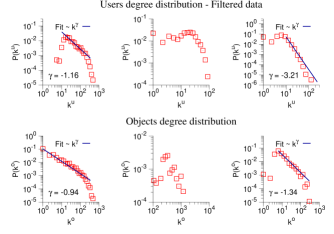
Figure 1: (Color online) Degree distributions of users (top panels) and objects (bottom panels) of the three data sets, respectively MovieLens (left), Jester Jokes (middle), and Fine Food (right).

Table 1: Summary statistics of the three databases used in the paper

	$N_{links}$	N x M	Rating	Thre-	$N_{links}$
		(used)	range	shold	Filtered
Movielens	100K	943 x 1,681	[1, 5]	3	90K
Jester Jokes	141K	2,000 x 100	[-10, 10]	0	57K
Fine Foods	95K	2,000 x 3,317	[1, 5]	3	83K

As a matter of fact, different similarity measures produce different distribution of similarity scores. In Fig. 2 and Fig. 3 we show the probability density functions of the MDW and BP similarities measures on the three investigated databases. The top panels of each figure report the distribution of user similarities, whereas the bottom panels correspond to object similarity. It is worth noting that the profile of the probability density functions is strongly dependent on the similarity measure adopted and is qualitatively different in the three data sets.

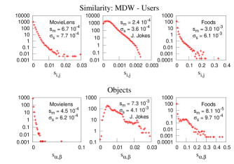
Figure 2: Distribution of the MDW similarity values for the three databases. The top panels show the probability density functions of users’ similarity whereas the bottom panels show the probability density functions of object similarity. Left, middle, and right columns refer to MovieLens, Jester Jokes, and Fine Food databases respectively.

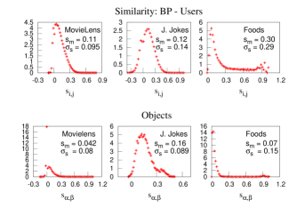
Figure 3: Distribution of the binary Pearson similarity values for the three databases. The top panels show the probability density functions of users’ similarity whereas the bottom panels show the probability density functions of object similarity. Left, middle, and right columns refer to MovieLens, Jester Jokes, and Fine Food databases respectively.

Validation. — In order to compare the performance of the proposed similarity measures with those of other existing similarity definitions, we split each data set into two sections. Starting from the adjacency matrix $A=\{a_{i,\alpha}\}$ representing all the user-object associations in a data set, we considered a subgraph $T=\{t_{i,\alpha}\}$ to be used to compute the similarity scores and recommendation lists for all the users (the so-called training set), while the remaining subgraph $W=\{a_{i,\alpha}\}\setminus\{t_{i,\alpha}\}=\{w_{i,\alpha}\}$ was used for validation. The recommendation lists obtained from the training sets are compared with the object selections included in the validation set, in order to check whether users have actually collected objects which are ranked high in their recommendation lists. In the following we report the results corresponding to training sets containing $90\%$ of all the edges of each data set, chosen at random, while the validation sets consist of the remaining $10\%$ of edges. Qualitatively similar results were obtained for different compositions of the training and validation sets.

A basic measure to quantify the performance of a recommendation method is the rank quality index $r$, which is computed as the average quality of recommendation over all the users of the data set. For each user $u_{i}$ we define the quality of the recommendation $r_{i}$ provided to $u_{i}$ as the average of the ratio

$$r_{i,\alpha}=w_{i,\alpha}\frac{L_{i,\alpha}}{M-k_{i}}.$$ (12)

computed over all the objects in the recommendation list of user $u_{i}$ which have actually been selected by $u_{i}$ in the validation set. Here $L_{i,\alpha}$ is the position of $o_{\alpha}$ in the recommendation list of $u_{i}$, where $L_{i,\alpha}=1,2,\ldots,$ if the object $o_{\alpha}$ is ranked first, second,$\dots$ etc. in the recommendation list of $u_{i}$. Consequently, better recommendations are associated to smaller values of $r_{i}=\sum_{\alpha}r_{i,\alpha}$. As we anticipated above, the rank quality index $r$ is the average of $r_{i,\alpha}$ over all the users in the data set:

$$r=\langle r_{i,\alpha}\rangle=\frac{\sum^{N}_{i=1}\sum^{M}_{\alpha=1}{r_{i,\alpha}}}{\sum^{N}_{i=1}\sum^{M}_{\alpha=1}{w_{i,\alpha}}}.$$ (13)

Another validation measure testing the accuracy of the predictions is the hitting rate, $hit(L)$, i.e., for all the users, the ratio between the number of collected objects included in the recommendation list of length $L$, and the number of objects effectively collected up to the possible maximum value $N\cdot L$. According to these definitions, a good recommendation method should minimize the value of $r$ and maximize the value of $hit(20)$.

For each data set, we considered $N_{e}=20$ independent realizations of the training set $T$, obtained by selecting uniformly at random $90\%$ of the edges in the data set, we constructed the recommendation list induced by each similarity measure, and computed the value of the rank quality index $r$ and of the hitting rate $hit(20)$. In the following we report the average values of $r$ and $hit(20)$ and their associated statistical errors (the standard deviations of the means), respectively denoted by $\langle r\rangle$, $\langle hit(20)\rangle$, $\sigma_{\langle r\rangle}$ and $\sigma_{\langle hit(20)\rangle}$. The mean values $\langle r\rangle$ and $\langle hit(20)\rangle$ obtained over the $N_{e}=20$ different realizations are shown in Table 2.

Table 2: Average rank quality index $\langle r\rangle$ and hitting rate $\langle hit(20)\rangle$ for the different recommendation methods on each of the three data sets. The mean is computed on $N_{e}=20$ different realizations. The standard deviation of the mean values is given in parenthesis. For each database we highlight in boldface the best result.

MovieLens	$\langle r\rangle$	$\sigma_{\langle r\rangle}$	$\langle hit(20)\rangle$	$\sigma_{\langle hit(20)\rangle}$
GRM	0.13821	(0.00038)	0.1928	(0.0041)
CF	0.11882	(0.00037)	0.2364	(0.0010)
NBI	0.10514	(0.00028)	0.2732	(0.0010)
MDW	0.10563	(0.00022)	0.2766	(0.0010)
BP	0.10728	(0.00032)	0.2708	(0.0009)
J	0.11442	(0.00035)	0.2568	(0.0010)
JesterJokes
GRM	0.30332	(0.00049)	0.6160	(0.0006)
CF	0.28718	(0.00051)	0.6712	(0.0008)
NBI	0.28422	(0.00045)	0.6775	(0.0012)
MDW	0.28087	(0.00037)	0.6806	(0.0010)
BP	0.23795	(0.00052)	0.6653	(0.0012)
J	0.28549	(0.00049)	0.6716	(0.0014)
Fine Foods
GRM	0.22263	(0.00073)	0.0891	(0.0004)
CF	0.01458	(0.00021)	0.7000	(0.0014)
NBI	0.01230	(0.00012)	0.7402	(0.0013)
MDW	0.01304	(0.00017)	0.7293	(0.0005)
BP	0.01173	(0.00010)	0.5777	(0.0009)
J	0.01534	(0.00013)	0.6990	(0.0009)

By analyzing the results summarized in Table 2 we see that the best results are obtained by different methods in different databases. Moreover the two indicators $\langle r\rangle$ and $\langle hit(20)\rangle$ always single out a different method as the best one. However, an overall analysis shows that the best recommendation methods are NBI (the best method according to $\langle r\rangle$ in the MovieLens database and the best method according to $\langle hit(20)\rangle$ in the Fine Foods database), MDW (the best method according to to $\langle hit(20)\rangle$ in the MovieLens and Fine Foods databases), and BP (the best method according to $\langle r\rangle$ in the Jester Jokes and in the Fine Foods databases). They clearly overcome the results obtained by GRM, CF, and Jaccard (J).

IV Hybrid object-user methods

The most important difference between the recommendation methods compared in Table 2 is that while NBI is based on a definition of similarity among objects, all the other methods make use of similarity measures defined between users.

In general, it is possible to define a transformation rule to obtain a similarity score between users starting from a similarity between objects, and viceversa. In fact, the similarity between objects $s^{\rm o}_{i,j}$ can be obtained from the similarity between users by appropriately swapping Latin indexes with Greek ones, and quantities defined for users with the analogous ones defined for objects:

$$s^{\rm u}_{i,j} \leftrightarrow s^{\rm o}_{\alpha,\beta}$$

$$i,j \leftrightarrow \alpha,\beta$$

$$N \leftrightarrow M.$$ (14)

The transformation rule is valid in both directions from user to objects and from objects to users.

We propose to define new recommendation scores by using the dual similarity measures obtained with the above defined transformation. For example, the recommendation value, which is the dual of Eq. (10) and is valid for objects instead of users, is obtained as:

$$v^{\rm o}_{i,\alpha}=\frac{\sum^{M}_{\beta=1,\beta\neq\alpha}{s^{\rm o}_{\alpha,\beta}\cdot a_{i,\beta}}}{\sum^{M}_{\beta=1,\beta\neq\alpha}{\left|s^{\rm o}_{\alpha,\beta}\right|}},$$ (15)

whereas the dual recommendation score of the NBI algorithm is

$$f^{\rm u}_{i,\alpha}=\sum^{N}_{l=1}{s^{\rm u,NBI}_{i,l}\cdot a_{l,\alpha}}.$$ (16)

It is interesting to note that according to the definition of the NBI we have

$$f^{\rm o}_{i,\alpha}=f^{\rm u}_{i,\alpha}=f_{i,\alpha}.$$ (17)

This relation can be verified by replacing $s^{\rm o,NBI}_{\alpha,\beta}$ (Eq. 3) with $s^{\rm u,NBI}_{i,l}=\frac{1}{k_{l}}\sum^{M}_{\beta=1}\frac{a_{i,\beta}a_{l,\beta}}{k_{\beta}}$ into the equations (11) and (16), respectively. Hence, NBI is invariant under the transformation rules of Eq. (14). It is interesting to investigate how the duality user/object similarity affects the quality of recommendation. To this aim, we propose to define a recommendation value $v_{i,\alpha}({\lambda})$ which is the result the convex combination of the two recommendation values $v_{i,\alpha}^{\rm u}$ and $v_{i,\alpha}^{\rm o}$ obtained from the similarity between users and between objects, respectively. In formula:

$$v_{i,\alpha}(\lambda)=(1-\lambda)v^{\rm u}_{i,\alpha}+\lambda v^{\rm o}_{i,\alpha},$$ (18)

where the relative weight of the user and object recommendation values is controlled by the parameter $\lambda\in[0,1]$, so that when $\lambda=0$ we recover the recommendation score induced by the similarity between users, while for $\lambda=1$ we have the recommendantion score corresponding to the similarity between objects. Our hypothesis, which is validated in the following, is that better recommendations can be obtained by appropriately tuning the value of $\lambda$.

The mean values $\langle r\rangle$ for different recommendation methods are reported in Fig. 4, where the three panels show the results obtained in the three data sets. It is worth noting that the NBI algorithm is independent of $\lambda$. In fact, by using Eq. (17) one verifies that

$$f_{i,\alpha}(\lambda)=(1-\lambda)f^{\rm u}_{i,\alpha}+\lambda f^{\rm o}_{i,\alpha}=f_{i,\alpha}.$$ (19)

In Fig. 4 we notice that the CF recommendation method performs poorly for almost all the values of $\lambda$, in all the three data sets. In the case of MovieLens, three recommendation methods (MDW, NBI and BP) perform in a similar way when only the user similarity measure is taken into account ($\lambda=0$) as we already noticed in the results summarized in Table 2. On the other hand, for $\lambda=1$, i.e., when only the object similarity measure is taken into account, the MDW method performs better than the others. In the case of the Fine Foods data set, the BP similarity performs slightly better than the others for $\lambda=0$ and for a relatively large range of $\lambda$ values. When $\lambda=1$, the recommendation with the MDW measure performs slightly better. Finally, in the Jester Jokes data set the BP similarity clearly outperforms all the others when $\lambda=0$, while for $\lambda=1$ all the methods provide similar results, with the only exception of the CF recommendation, whose performance is much worse.

The richness of profiles observed in Fig. 4 suggests that the performance of a recommendation method depends both on the specific database and on the specific linear combination of user and object recommendation values adopted. Quite often, the best recommendation is not the one corresponding to $\lambda=0$ or $\lambda=1$. Some methods perform better at the user limit ($\lambda=0$), others at the object limit ($\lambda=1$), some of them for an intermediate value of $\lambda$. Moreover, the specific shape of $\langle r\rangle$ as a function of $\lambda$ actually depends on the database. We would like to stress two interesting aspects of these results. First, some methods exhibit a convex profile of $\langle r\rangle$ as a function of $\lambda$, where the minimum indicates the best linear combination of user and object recommendation values. Second, the variability of the values of $\langle r\rangle$ obtained by different recommendation systems is much higher for $\lambda=1$ than for $\lambda=0$.

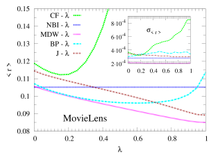
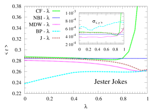
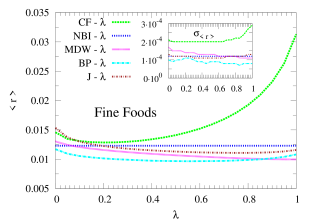
Figure 4: (Color online) Average rank quality index $\langle r\rangle$ for the different recommendation methods as a function of the user/object parameter $\lambda$. The insets report the corresponding standard errors of the mean.

V Impact of randomness

In this Section we analyse the robustness of recommendation systems against the presence of different sources of noise in the data sets. We consider three different kinds of randomization. In the first scenario we add a certain amount of random edges to the bipartite graph, mimicking erroneously reported user selections. In the second case we rewire a given percentage of the edges of the bipartite network by maintaining the degree of users unaltered (while the degree distribution of object is in general modified). Finally, in the third case we rewire a fraction of the edges of the graph by maintaining unaltered both the user and object degree distribution.

For the sake of simplicity, we show the results obtained for the three randomizing methods only for the MovieLens database. In Fig. 5 we show the average rank quality index for the different methods with $\lambda=0$ as a function of the percentage of edges randomly added or rewired. As expected, $\langle r\rangle$ is an increasing function of the percentage of noise, signalling a degradation of the recommendation performance. However, the actual profile of $\langle r\rangle$ depends on the specific recommendation method used. In fact, several curves crosses at different values of the induced randomness. This is clearly observed for the first and second kinds of randomization.

We performed the same analysis also on the Jester Jokes and Fine Foods databases, and we report in Fig. 6 the results corresponding to the first type of randomization (addition of a fraction of random edges). The results show a prominent role of the BP similarity measure, which seems the most robust in dealing with noisy data sets.

Our findings suggest that the BP similarity measure is a good candidate to provide good and robust recommendations in databases where there is a high degree of uncertainty about the validity of records. In fact, while the use of the BP similarity does not give substantially better recommendation prediction in databases like MovieLens and Fine Foods, its performance is consistently higher in the case of Jester Jokes.

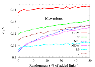
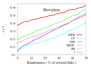
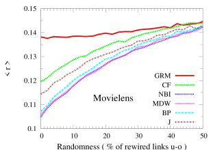
Figure 5: (Color online) Mean validation values as a function of noise in the MovieLens database. The three panels correspond, respectively, to the addition of edges at random (top) and to edge rewirings which maintain unaltered only the user degree sequence (middle) or both the user and object degree sequences (bottom).

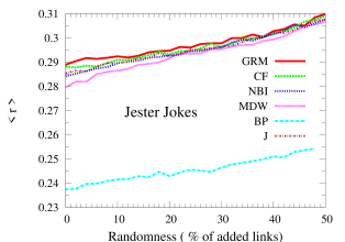
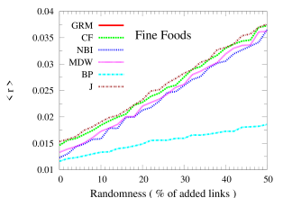
Figure 6: (Color online) Mean validation values for some different methods as a function of the randomness with the Jester jokes (top panel) and Fine Foods (bottom panel) databases.

VI Conclusions

We have considered three real-world users/items bipartite networks, we have investigated the performance of several traditional recommendation methods recently presented in the literature, and we have proposed two new similarity measures which take into account the heterogeneity of users and objects degrees. We showed that these two new similarity indexes can outperform traditional recommendation systems in most of the cases, even if there is a clear dependence of the results on the structural characteristics of the data set under study.

Then, we focused on hybrid recommendation systems based on the convex combination of the recommendation scores induced by the similarity between users and objects, parametrised by a coefficient $\lambda$. We showed that different outcomes can be obtained in personalized recommendation methods by using similarity between users, or between objects, or a combination of the two. In some cases, the quality of recommendation as measured by the average rank quality index $r$ is a convex function of the parameter $\lambda$. This means that the combination of different recommendation scores might actually provide better performance with respect than the employment of user or object similarities alone and, more importantly, that depending on the data set at hand, the quality of recommendation can be actually optimised through an appropriate tuning of $\lambda$. Conversely, for some similarity measures we observed a monotonically decreasing dependence of $\langle r\rangle$ on $\lambda$, so that the best recommendation is obtained by using an object-based similarity. We finally investigated the robustness of recommendation systems to the addition and rewiring of edges, and the results suggested that the Binary Person correlation similarity can consistently outperform other similarity measures in noisy data sets.

Although we do not observe a specific recommendation method outperforming all the others in all conditions and for all the data sets considered, it seems that recommendations based on MDW and BP are able to produce better results than those using other similarity measures. However, our results show that the performance of the recommendation methods depends on both the specific investigated database and on the way similarities between users and objects are used to derive recommendation scores.

- (1) G. Adomavicius and A. Tuzhilin, IEEE 17 734 (2005).
- (2) L. Lü, M. Medo, C.-H. Yeung, Y.-C. Zhang, and Z.-K. Zhang, Phys. Rep. 519 1 (2012).
- (3) B. Sarwar, G. Karypis, J. Konstan, and J. Riedl. Item-based collaborative filtering. Proc. Int. Conf. WWW10, ACM 1-58113-348-0/01/0005, 285 (2001)
- (4) D. Goldberg, D. Nichols, B.M. Oki, D. Terry, Commun. ACM 35 61 (1992)
- (5) J.B. Schafer, D. Frankowski, J. Herlocker, S. Sen, Collaborative filtering recommender systems. In: The adaptive web Springer 291 (2007).
- (6) Y.-C. Zhang, M. Blatter, and Y.-K. Yu, Phys. Rev. Lett. 99 154301 (2007).
- (7) T. Zhou, R.Q. Su, R.R. Liu, L.L. Jiang, B.H. Wang, and Y.-C. Zhang, New J. of Phys. 11 123008 (2009).
- (8) T. Zhou, J. Rien, M. Medo, and Y.-C. Zhang, Phys. Rev. E 76 046115 (2007).
- (9) L. Lü, W. Liu, Phys. Rev. E 83 066119 (2011)
- (10) T. Zhou, Z. Kuscsik, J.-G. Liu, M. Medo, J.R. Wakeling, and Y.-C. Zhang, PNAS 107 4511 (2010).
- (11) T.Q. Qiu, Z.-K Zhang, and G. Chen,PloSONE 8 1 (2013).
- (12) X. Zhu, H. Tian, and S. Cai, arXiv:1405.4095v1 [cs.IR] (2014).
- (13) K. Pearson, Proceedings of the Royal Society of London 58 240 (1895).
- (14) L. Lü, T. Zhou, Physica A 390 1150 (2011).
- (15) P. Jaccard, Bull. Soc. Vaud. Sci. Nat. 37 547 (1901).
- (16) R.-R. Liu, C.-X. Jia, T. Zhou, D. Sun, B.-H. Wang, Physica A 388 462 (2009).
- (17) Q. Guo, R. Leng, K. Shi, and J.G. Liu, Eur. Phys. J. B 85: 286 (2012)
- (18) M. Tumminello, S. Miccichè, L.J. Dominguez, G. Lamura, M.G. Melchiorre, M. Barbagallo, and R.N. Mantegna, PlosONE 6(9) e23377 (2011)
- (19) V. Hatzopoulos, G. Iori, R.N. Mantegna, S. Miccichè, and M. Tumminello: Quantitative Finance DOI:10.1080/14697688.2014.969889 (2014)