Numerical solution of the Boltzmann equation for trapped Fermi gases with in-medium effects

Abstract

Using the test-particle method, we solve numerically the Boltzmann equation for an ultra-cold gas of trapped fermions with realistic particle number and trap geometry in the normal phase. We include a mean-field potential and in-medium modifications of the cross-section obtained within a T matrix formalism. After some tests showing the reliability of our procedure, we apply the method to realistic cases of practical interest, namely the anisotropic expansion of the cloud and the radial quadrupole mode oscillation. Our results are in good agreement with experimental data. Although the in-medium effects significantly increase the collision rate, we find that they have only a moderate effect on the anisotropic expansion and on frequency and damping rate of the quadrupole mode.

I Introduction

Ultracold gases of trapped atoms offer unique opportunities to study Fermionic many-body systems under clean and adjustable conditions. In particular, by tuning the magnetic field around a Feshbach resonance, one can realize either a repulsive or an attractive interaction, passing through the “unitary limit” where the scattering length $a$ diverges. Especially this “unitary Fermi gas” has attracted a lot of attention because it has “universal” properties (there is no scale depending on the interaction strength) and it has some similarities with completely different systems such as low-density neutron matter. A very interesting aspect of these strongly correlated atomic gases are the different dynamical regimes they can be in: they can be superfluid or normal-fluid, and in the normal-fluid phase hydrodynamic to collisionless behavior can be realized depending on interaction strength and temperature. Experimentally, the transition between these regimes has been seen, e.g., by studying the frequency and damping rates of the radial quadrupole mode Wright2007 ; Riedl2008 . Another source of information is the free expansion (i.e., after the trap is switched off) of an anisotropic gas, which is very different in the ballistic and in the hydrodynamic regime OHara2002 ; Menotti2002 ; Pedri2003 ; Schaefer2010 . Surprisingly, the low viscosity of the unitary Fermi gas observed in this way Cao2011 ; Elliott2014a ; Elliott2014b ; Joseph2014 seems to indicate some analogies even with the quark-gluon plasma created in ultrarelativistic heavy-ion collisions Schaefer2009 .

In the normal phase, the transition between hydrodynamic and collisionless regimes can be described by the Boltzmann equation Toschi2003 ; Massignan2005 ; BruunSmith2007_scissors ; Riedl2008 ; Chiacchiera2009 ; Lepers2010 ; Chiacchiera2011 ; WuZhang2012 . The test-particle method for the numerical solution of the Boltzmann equation has been used for many years in the field of heavy-ion collisions Bertsch1988 and more recently also for ultracold atoms Toschi2003 ; Toschi2004 ; Lepers2010 ; Wade2011 ; Goulko2011 ; Goulko2012 . In this article, we extend the method developed in Lepers2010 in order to simulate realistic systems (trap geometry and particle number). At the same time, we include in-medium effects into the calculation, namely the “mean-field” potential Chiacchiera2009 ; Pantel2012 and the in-medium cross-section Riedl2008 ; BruunSmith2005 ; Chiacchiera2009 ; BluhmSchaefer2014 , obtained within a T matrix theory.

In Sec. II, we briefly recall the Boltzmann equation with in-medium effects and explain the test-particle method we use to solve it numerically, concentrating mainly on elements which are new as compared to LABEL:Lepers2010. Then we describe in Sec. III some tests of the reliability of the code. In Sec. IV, we discuss as first applications of the code the simulation of different anisotropic expansion experiments of the Duke group Cao2011 ; Elliott2014a and the radial quadrupole mode as measured at Innsbruck Riedl2008 . In Sec. V we conclude and discuss perspectives for future work.

Throughout the article, we use units with $\hbar=k_{B}=1$ ($\hbar=$ reduced Planck constant, $k_{B}=$ Boltzmann constant).

II Methods

II.1 Boltzmann equation

We study a two-component $(s\in\{\uparrow,\downarrow\}$) ultra-cold gas of $N=N_{\uparrow}+N_{\downarrow}$ atoms of mass $m$ with attractive interaction (scattering length $a<0$) in an external potential $V_{\text{trap}}(\bm{\mathrm{r}},t)$. Even if we will restrict the numerical implementation of the in-medium effects to the case of a spin balanced ($N_{\uparrow}=N_{\downarrow}$) system, we keep the notation general. We will only consider the normal-fluid phase, i.e., temperatures $T$ above the superfluid transition temperature $T_{c}$. In this case, the dynamics of the system can be described with a distribution function $f_{s}(\bm{\mathrm{r}},\bm{\mathrm{p}},t)$ which satisfies the Boltzmann equation

$$\frac{\partial f_{s}}{\partial t}+\frac{\bm{\mathrm{p}}}{m}\cdot\frac{\partial f_{s}}{\partial\bm{\mathrm{r}}}+\bm{\mathrm{F}}_{s}(\bm{\mathrm{r}},t)\cdot\frac{\partial f_{s}}{\partial\bm{\mathrm{p}}}=-I_{s}\,,$$ (1)

where $I_{s}$ is the collision integral (see below) and $\bm{\mathrm{F}}_{s}=\bm{\mathrm{F}}_{\text{trap}}+\bm{\mathrm{F}}_{{\text{mf}},s}$ is the sum of the forces resulting from the external potential $V_{\text{trap}}(\bm{\mathrm{r}},t)$ and from the mean field $U_{s}(\bm{\mathrm{r}},t)$.

The trap potential $V_{\text{trap}}$ is essentially given by a time independent anisotropic harmonic trap

$$V_{\text{trap}}(\bm{\mathrm{r}})=\frac{1}{2}m(\omega_{x}^{2}x^{2}+\omega_{y}^{2}y^{2}+\omega_{z}^{2}z^{2})\,,$$ (2)

(in the cylindrically symmetric case, we use $\omega_{r}=\omega_{x}=\omega_{y}$) which defines the time and length scales $\bar{\omega}^{-1}=(\omega_{x}\omega_{y}\omega_{z})^{-1/3}$ and $\bar{L}_{\text{ho}}=(m\bar{\omega})^{-1/2}$. In addition to the static harmonic potential, $V_{\text{trap}}$ can have a time dependent contribution, e.g., in order to excite a collective mode ($V_{\text{exc}}$).

The density per spin state and the number of atoms of species $s$ are obtained from the distribution function as

$$\rho_{s}(\bm{\mathrm{r}},t) =\int\frac{d^{3}p}{(2\pi)^{3}}f_{s}(\bm{\mathrm{r}},\bm{\mathrm{p}},t)\,, N_{s} =\int d^{3}r\rho_{s}(\bm{\mathrm{r}},t)\,.$$ (3)

The right-hand side (r.h.s.) of the Boltzmann equation (1) describes the collisions between particles of opposite spin. It thus depends on the differential scattering cross section $d\sigma/d\Omega$. If we consider, e.g., the $\uparrow$ component, it reads explicitly:

$$I_{\uparrow}=\int\frac{d^{3}p_{\downarrow}}{(2\pi)^{3}}\int d\Omega\frac{d\sigma}{d\Omega}\frac{|\bm{\mathrm{p}}_{\uparrow}-\bm{\mathrm{p}}_{\downarrow}|}{m}\\ \times\left[f_{\uparrow}f_{\downarrow}(1-f_{\uparrow}^{\prime})(1-f_{\downarrow}^{\prime})-f_{\uparrow}^{\prime}f_{\downarrow}^{\prime}(1-f_{\uparrow})(1-f_{\downarrow})\right],$$ (4)

where, in the first term, $\bm{\mathrm{p}}_{s}$ and $\bm{\mathrm{p}}_{s}^{\prime}$ are the incoming and outgoing momenta, respectively, while in the second term, the roles are exchanged. We adopted the short-hand notation $f_{s}=f_{s}(\bm{\mathrm{r}},\bm{\mathrm{p}}_{s},t)$ and $f_{s}^{\prime}=f_{s}(\bm{\mathrm{r}},\bm{\mathrm{p}}_{s}^{\prime},t)$.

Since we consider only $s$-wave interactions, the cross section does not depend on the scattering angle $\Omega$ and we simply have $\sigma=4\pi\,d\sigma/d\Omega$. In free space, it depends only on the relative momentum $q=|\bm{\mathrm{p}}_{\uparrow}-\bm{\mathrm{p}}_{\downarrow}|/2$ and is given by

$$\sigma=\sigma_{0}(q)=\frac{4\pi a^{2}}{1+(qa)^{2}}.$$ (5)

When in-medium effects are taken into account (see Sec. II.3), there is of course no such simple form.

II.2 Test-particle method

In this article, we use the test-particle method described, e.g., in Lepers2010 , but generalized to the case $\nu<1$, where $\nu=\tilde{N}/N$ is the number of test particles per atom. This case is of course of practical interest since it allows us to simulate a large number $N$ of real particles with a smaller number $\tilde{N}$ of test particles. However, the problem of a correct sampling of the phase space immediately arises.

As discussed in detail in Lepers2010 , the main problem when reducing the number of test particles is that one cannot resolve any more the step of the distribution function at the Fermi surface. This is, however, crucial for the description of Pauli blocking of collisions. The resolution can be reduced at finite temperature since the Fermi surface gets smoothed out. In the unitary limit, the superfluid transition temperature $T_{c}$ is already of the order of $\sim 0.3\,T_{F}$, where $T_{F}$ is the Fermi temperature defined in the usual way by $T_{F}=(3N)^{1/3}\bar{\omega}$ (which is lower than the local Fermi temperature in the center of the trap). Since we are anyway forced to stay above $T_{c}$, we can work with a smaller number of test particles.

The test-particle method consists of writing the (non-equilibrium) distribution function as

$$f_{s}(\bm{\mathrm{r}},\bm{\mathrm{p}},t)=\frac{1}{\nu}\sum_{i_{s}}\delta(\bm{\mathrm{r}}-\bm{\mathrm{r}}_{i_{s}}(t))\delta(\bm{\mathrm{p}}-\bm{\mathrm{p}}_{i_{s}}(t)),$$ (6)

where $\bm{\mathrm{r}}_{i}$ and $\bm{\mathrm{p}}_{i}$ are the position and momentum of the $i$-th test particle at time $t$. In practice, the first $\tilde{N}_{\uparrow}=\nu N_{\uparrow}$ test particles represent atoms with spin $\uparrow$, while the remaining $\tilde{N}_{\downarrow}=\nu N_{\downarrow}$ test particles represent atoms with spin $\downarrow$. To simplify the notation, we use the convention that the index $i_{\uparrow}$ runs from $1$ to $\tilde{N}_{\uparrow}$, the index $i_{\downarrow}$ from $\tilde{N}_{\uparrow}+1$ to $\tilde{N}$, and the index $i$ from $1$ to $\tilde{N}=\tilde{N}_{\uparrow}+\tilde{N}_{\downarrow}$.

With the test-particle method, the l.h.s. of the Boltzmann equation is replaced by a set of $6\tilde{N}$ classical equations of motion

$$\dot{\bm{\mathrm{r}}}_{i_{s}}(t)=\frac{\bm{\mathrm{p}}_{i_{s}}(t)}{m}\,,\quad\dot{\bm{\mathrm{p}}}_{i_{s}}(t)=\bm{\mathrm{F}}_{s}(\bm{\mathrm{r}}_{i_{s}}(t),t)\,.$$ (7)

To solve these equations, a particular attention has to be paid to the efficiency and numerical accuracy. For our simulations, we use the velocity Verlet algorithm as in Lepers2010 .

The collision term is simulated by scattering two test particles of opposite spin by a random angle if their distance becomes smaller than that corresponding to the cross section (see Lepers2010 for details). To take Pauli blocking into account, the collision is only performed with a probability given by $(1-f_{\uparrow}^{\prime})(1-f_{\downarrow}^{\prime})$.

Of course, the $\delta$ functions in Eq. (6) cannot be used to obtain meaningful numbers for the Pauli-blocking factors $(1-f_{\uparrow}^{\prime})(1-f_{\downarrow}^{\prime})$. The usual way to avoid this problem is to consider Gaussian distributions in $\bm{\mathrm{r}}$ and $\bm{\mathrm{p}}$ spaces instead of the Dirac ones. In the calculation of the Pauli-blocking factors, we therefore replace $\delta(\bm{\mathrm{r}}-\bm{\mathrm{r}}_{i})\delta(\bm{\mathrm{p}}-\bm{\mathrm{p}}_{i})$ with $g_{r}(\bm{\mathrm{r}}-\bm{\mathrm{r}}_{i})g_{p}(\bm{\mathrm{p}}-\bm{\mathrm{p}}_{i})$, where

$$g_{p}(\bm{\mathrm{p}})=\frac{\exp(-p^{2}/w_{p}^{2})}{(\sqrt{\pi}w_{p})^{3}},$$ (8)

and

$$g_{r}(\bm{\mathrm{r}})=\frac{\exp(-x^{2}/w_{r,x}^{2}-y^{2}/w_{r,y}^{2}-z^{2}/w_{r,z}^{2})}{(\sqrt{\pi}\bar{w}_{r})^{3}}.$$ (9)

In contrast to the Gaussian used in Lepers2010 , the above Gaussian $g_{r}$ takes explicitly into account the deformed shape of the gas. To be specific, the widths appearing in the above equation are defined from an average width $\bar{w}_{r}$ as

$$w_{r,j}=\frac{\bar{\omega}}{\omega_{j}}\bar{w}_{r},$$ (10)

where $j\in\{x,y,z\}$. In this way we exploit the fact that the typical length scales on which the distribution function varies, given by the trap potential, can be very different in the three spatial directions.

The values of $\bar{w}_{r}$ and $w_{p}$ must be chosen such that they smooth the statistical fluctuations due to the finite number of test particles but resolve the structure of the distribution function $f_{s}$ (see Lepers2010 for details). The parameters we use in the present paper are given in Table 1.

Table 1: Numerical parameters used in the simulations shown in the figures.

Figs.		1, 2, 6–8	3–5
$\tilde{N}$		$5\cdot 10^{4}$	$1\cdot 10^{5}$
$\Delta t$	($\bar{\omega}^{-1}$)	$0.02$	$0.01$
$\bar{w}_{r}$	($\bar{L}_{\text{ho}}$)	$3$	$3$
$w_{p}$	($\bar{L}_{\text{ho}}^{-1}$)	$3$	$3$
$\bar{w}$	($\bar{L}_{\text{ho}}$)	$2$	$2$

Another improvement w.r.t. LABEL:Lepers2010 concerns the inclusion of the in-medium cross section $\sigma$ and of the mean field $U_{s}$. For simplicity, we assume that these quantities can be calculated at a local equilibrium characterized by time-dependent effective local chemical potentials and temperature, $\mu^{*}_{s}(\bm{\mathrm{r}},t)$ and $T^{*}(\bm{\mathrm{r}},t)$. In practice, it is more convenient to parameterize $\sigma$ and $U$ in terms of the densities $\rho_{s}$ and of the kinetic-energy density, $\epsilon$, which are related by a one-to-one correspondence to $\mu^{*}_{s}$ and $T^{*}$:

$$\rho_{s}=\int\frac{d^{3}k}{(2\pi)^{3}}\frac{1}{e^{(k^{2}/2m+U_{s}-\mu^{*}_{s})/T^{*}}+1}\,,$$ (11)

$$\epsilon=\sum_{s}\int\frac{d^{3}k}{(2\pi)^{3}}\frac{k^{2}/2m}{e^{(k^{2}/2m+U_{s}-\mu^{*}_{s})/T^{*}}+1}\,.$$ (12)

When one calculates $\rho_{s}$ and $\epsilon$ from the test-particle distribution, it is enough to introduce an averaging in $\bm{\mathrm{r}}$ space (contrary to the case of the Pauli-blocking factors discussed above, where also averaging in $\bm{\mathrm{p}}$ space is needed). Again, we use Gaussians for this purpose, with widths $w_{j}$ which are derived from an average width $\bar{w}$ analogously to Eq. (10). The width $\bar{w}$ can be chosen smaller than the width $\bar{w}_{r}$ used in the Pauli-blocking factors, because in the density and energy density we sum over all momenta and therefore the statistical fluctuations are smaller. During the simulation, the averaged densities and kinetic-energy density are computed as

$$\tilde{\rho}_{s}(\bm{\mathrm{r}},t)=\frac{1}{\nu}\sum_{i_{s}}g(\bm{\mathrm{r}}-\bm{\mathrm{r}}_{i_{s}})\,,$$ (13)

$$\tilde{\epsilon}(\bm{\mathrm{r}},t)=\frac{1}{\nu}\sum_{i}g(\bm{\mathrm{r}}-\bm{\mathrm{r}}_{i})\frac{[\bm{\mathrm{p}}_{i}-m\tilde{\bm{\mathrm{v}}}(\bm{\mathrm{r}},t)]^{2}}{2m}\,.$$ (14)

Note that $\epsilon$ is defined in the frame moving with the local average velocity

$$\tilde{\bm{\mathrm{v}}}(\bm{\mathrm{r}},t)=\frac{1}{\nu\tilde{\rho}(\bm{\mathrm{r}},t)}\sum_{i}g(\bm{\mathrm{r}}-\bm{\mathrm{r}}_{i})\frac{\bm{\mathrm{p}}_{i}}{m}\,,$$ (15)

where $\tilde{\rho}=\tilde{\rho}_{\uparrow}+\tilde{\rho}_{\downarrow}$. These quantities are calculated after every time step and stored on a three-dimensional (3d) grid.

Since the mean fields $U_{s}$ are now functions of the smoothed densities $\tilde{\rho}_{s}$, one would violate Newton’s third law if one computed the corresponding force directly as $\bm{\mathrm{F}}_{{\text{mf}},s}=-\bm{\nabla}U_{s}$. Following Urban2012 , one has to average the force using the same Gaussians $g$ as in the calculation of $\tilde{\rho}_{s}$, i.e., the contribution to the force on a test particle $i_{s}$ caused by its interactions with all the other test particles is given by

$$\bm{\mathrm{F}}_{{\text{mf}},s}(\bm{\mathrm{r}}_{i_{s}},t)=-\frac{\partial}{\partial\bm{\mathrm{r}}_{i_{s}}}\tilde{U}_{s}(\bm{\mathrm{r}}_{i_{s}},t)\\ =-\frac{\partial}{\partial\bm{\mathrm{r}}_{i_{s}}}\int d^{3}rg(\bm{\mathrm{r}}_{i_{s}}-\bm{\mathrm{r}})U_{s}(\bm{\mathrm{r}},t)\,.$$ (16)

It is straight-forward to show that with this prescription the sum of all interaction forces would be exactly zero, as required by momentum conservation, if the mean fields $U_{s}$ were only functions of the densities $\tilde{\rho}_{s}$. However, since the mean fields depend also on $\tilde{\epsilon}$, this relation is probably only approximately fulfilled (see also Sec. III.1).

II.3 In-medium cross section

Since the cross section governs the collisions, the introduction of in-medium effects may have important consequences in the dynamics of the system. Following Chiacchiera2009 , where a T-matrix approximation is used to calculate the in-medium correlations, we write the expression for the cross section as

$$\frac{d\sigma_{\text{med}}(\bm{\mathrm{k}},\bm{\mathrm{q}})}{d\Omega}=\left|\frac{m}{4\pi}\Gamma(\omega,\bm{\mathrm{k}})\right|^{2},$$ (17)

where $\omega=k^{2}/4m+q^{2}/m-2\bar{\mu}$ is the total energy (w.r.t. $2\bar{\mu}=\mu_{\uparrow}+\mu_{\downarrow}$), $\bm{\mathrm{k}}=\bm{\mathrm{p}}_{\uparrow}+\bm{\mathrm{p}}_{\downarrow}$ and $\bm{\mathrm{q}}=(\bm{\mathrm{p}}_{\uparrow}-\bm{\mathrm{p}}_{\downarrow})/2$ are total and relative momenta of the colliding particles with spin $\uparrow$ and $\downarrow$. The in-medium T matrix $\Gamma$ is defined as

$$\Gamma(\omega,\bm{\mathrm{k}})=\frac{4\pi a}{m}\,\frac{1}{1+iaq-\frac{4\pi a}{m}J(\omega,\bm{\mathrm{k}})}\,,$$ (18)

with $q=\sqrt{m(\omega+2\bar{\mu})-k^{2}/4}$. The medium contribution to the non-interacting two-particle Green’s function reads

$$J(\omega,\bm{\mathrm{k}})=-\int\frac{d^{3}q^{\prime}}{(2\pi)^{3}}\frac{f_{0}(\xi_{\bm{\mathrm{k}}/2+\bm{\mathrm{q}}^{\prime}}^{\uparrow})+f_{0}(\xi_{\bm{\mathrm{k}}/2-\bm{\mathrm{q}}^{\prime}}^{\downarrow})}{\omega-\xi_{\bm{\mathrm{k}}/2+\bm{\mathrm{q}}^{\prime}}^{\uparrow}-\xi_{\bm{\mathrm{k}}/2-\bm{\mathrm{q}}^{\prime}}^{\downarrow}+i\eta}.$$ (19)

In the above equation, $f_{0}(\xi)=1/(e^{\beta\xi}+1)$ is the Fermi function with $\beta=1/T$, and $\xi_{\bm{\mathrm{k}}}^{s}=k^{2}/2m-\mu_{s}$ represents the single-particle energy (measured w.r.t. the chemical potential $\mu_{s}$) of an atom with spin $s$. As usual, the limit $\eta\to 0$ is implicit.

This approach has already been used in Refs. Chiacchiera2009 ; Chiacchiera2011 to study collective modes in an unpolarized gas ($N_{\uparrow}=N_{\downarrow}$). Actually, since the standard (non self-consistent) T-matrix approximation fails in the polarized case, we will include the medium effects only in the unpolarized case.

Strictly speaking, the in-medium cross section given above is only valid for a gas described by a thermal equilibrium distribution $f_{0}$, characterized by chemical potentials $\mu_{s}$ and a temperature $T$. As mentioned in the preceding subsection, we use this cross section also in the non-equilibrium case, calculating it with the local effective chemical potentials $\mu^{*}_{s}$ and effective temperature $T^{*}$ which give the same densities $\rho_{s}$ and energy density $\epsilon$ as the actual (non-equilibrium) distribution function $f$. While this is exact in the linear response regime, it is of course only an approximation in situations far from equilibrium.

Including in-medium effects in a simulation implies a huge increase of the computation time: in order to decide whether a collision between an $\uparrow$ and a $\downarrow$ particle is allowed, the first criterion is given by the relative distance (and thus the cross-section $\sigma_{\text{med}}$) between the test particles. Therefore, $\sigma_{\text{med}}$ (which depends on the relative and total momenta of the two colliding test particles) has to be determined $\tilde{N}_{\uparrow}\tilde{N}_{\downarrow}$ times at each time step. The computation of the real part of $J$ involves a numerical integration Chiacchiera2009 , and therefore it would be much too time-consuming to include the exact in-medium cross section into the simulation. It is clearly necessary to use a simple parameterization of the cross section which can be evaluated quickly. More details are given in Appendix A.

II.4 Mean-field potential

In order to be consistent, we also have to take into account the in-medium effects in the left-hand side of the Boltzmann equation, i.e., the mean-field potential $U$. Following LABEL:Chiacchiera2009, we calculate it as

$$U=\operatorname{Re}\Sigma(0,k_{\bar{\mu}^{*}})\,,$$ (20)

where $\Sigma$ is the self-energy in ladder approximation $k_{\bar{\mu}^{*}}=\sqrt{2m\operatorname{max}(\bar{\mu}^{*},0)}$ (see LABEL:Chiacchiera2009 for further details). Like the cross section, this mean-field depends on $\bm{\mathrm{r}}$ and $t$ through the effective chemical potential $\bar{\mu}^{*}$ and temperature $T^{*}$ determined from the density $\bar{\rho}$ [since we can calculate the mean field only in the unpolarized case, we use $\bar{\rho}=(\rho_{\uparrow}+\rho_{\downarrow})/2$] and energy density $\epsilon$. In practice, for a given $a$, we tabulate it directly as function of $\bar{\rho}$ and $\epsilon$, using the Nozières-Schmitt-Rink relation between $\bar{\rho}$ and $\bar{\mu}^{*}$ (cf. Ref. [15]).

II.5 Initialization

The last point concerns the initialization process. The system is initialized according to an equilibrium Fermi distribution (the same for $\uparrow$ and $\downarrow$ particles since we limit ourselves to balanced systems for the moment) for a given temperature $T$

$$f_{\text{eq},s}(\bm{\mathrm{r}},\bm{\mathrm{p}})=\frac{1}{e^{\left[p^{2}/2m+V_{\text{trap}}(\bm{\mathrm{r}})+\tilde{U}(\bm{\mathrm{r}})-\mu\right]/T}+1}.$$ (21)

Note that the mean field $\tilde{U}$ entering here is the one folded with the Gaussian $g$ as described in Sec. II.2, and it has to be calculated self-consistently from the folded density and energy density $\tilde{\rho}$ and $\tilde{\epsilon}$, otherwise the initial distribution would not be stationary under the time evolution of the code Urban2012 .

In practice, we store $\rho$, $\tilde{\rho}$, $\epsilon$, $\tilde{\epsilon}$, $U$, and $\tilde{U}$ on a 3d grid. Starting from the density profile of an ideal Fermi gas, we iterate them simultaneously with $\mu$ in order to converge to a self-consistent solution with the correct particle number. In the end, because of the attractive mean field, we obtain a density profile that is more concentrated in the trap center (cf. Fig. 3 of LABEL:Chiacchiera2009) and a chemical potential that is lower than that of the ideal Fermi gas.

Once $\mu$ and $\tilde{U}$ are determined, the positions $\bm{\mathrm{r}}_{i}$ and momenta $\bm{\mathrm{p}}_{i}$ are initialized randomly according to the distribution (21), as in LABEL:Lepers2010.

III Tests of reliability and accuracy

III.1 Sloshing mode

The first test to check the consistency of our numerical approach concerns the particle propagation (left-hand side of the Boltzmann equation). This has already been done in LABEL:Lepers2010 but without mean-field. Therefore, we will concentrate on the implementation of $U(\bm{\mathrm{r}},t)$. One conclusive way to check this is to excite the sloshing mode (center-of-mass oscillation). As mentioned in Pantel2012 , the mean-field potential must not have any effect on the sloshing frequency when the trapping potential is harmonic. For instance, if the mode along the $x$ direction is excited, the frequency of the sloshing mode must be $\omega_{x}$ (Kohn’s theorem Kohn1961 ).

Figure 1

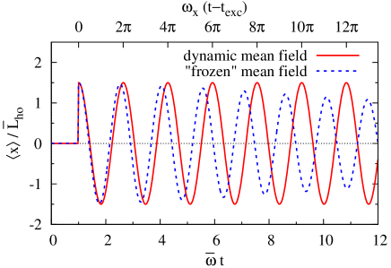
Figure 1: Simulation of the sloshing mode in $x$ direction in a realistic system whose parameters are given in Table 2 at $1/k_{F}a=-0.1$ and $T/T_{F}=0.4$. The result of the full calculation (solid line) is compared with the result obtained with a “frozen” mean field (dashed line, see text).

shows the result for the sloshing mode for a realistic system whose parameters are listed in Table 2.

Table 2: Parameters of the quadrupole mode experiment of LABEL:Riedl2008.

$\omega_{r}/2\pi$	(Hz)	1800
$\omega_{z}/2\pi$	(Hz)	32
$N$		$6\cdot 10^{5}$

The excitation has been produced at $\bar{\omega}t_{\text{exc}}=1$ by a global shift of all particle positions by $1.5\bar{L}_{\text{ho}}$ in $x$ direction. Note that this shift is comparable to the cloud width $\sqrt{\langle x^{2}\rangle}\approx 1.8\bar{L}_{\text{ho}}$, i.e., we are no longer in the linear response regime. The solid line corresponds to the full simulation, which takes the mean field and the in-medium cross section into account. We observe an undamped oscillation of the center of mass $\langle x\rangle$ with frequency $\omega_{x}$ (cf. upper scale in Fig. 1), in perfect agreement with Kohn’s theorem.

In order to show that this is indeed a non-trivial test of the calculation of the mean field $U(\bm{\mathrm{r}},t)$, we show for comparison as the dashed line the result one obtains if the mean field is “frozen” (i.e., not changed during the time evolution) at its initial value $U(\bm{\mathrm{r}},t=0)$. In this case, the oscillation of the cloud is faster than $\omega_{x}$ and damped, because the total potential $V_{\text{trap}}+U$ is deeper than $V_{\text{trap}}$ and anharmonic.

We thus have demonstrated that the particle propagation in the presence of the mean field, and the calculation of the mean field from the distribution function, are well described in our code.

III.2 Collision rate

A good way to check the precision of the simulation of the collision term is to compare the collision rate per particle in equilibrium given by the code with its exact value obtained directly from the definition

$$\gamma=\frac{1}{N}\int d^{3}r\int\frac{d^{3}p_{\uparrow}}{(2\pi)^{3}}\int\frac{d^{3}p_{\downarrow}}{(2\pi)^{3}}\int d\Omega\frac{d\sigma}{d\Omega}\frac{|\bm{\mathrm{p}}_{\uparrow}-\bm{\mathrm{p}}_{\downarrow}|}{m}\\ \times f_{\uparrow}f_{\downarrow}(1-f_{\uparrow}^{\prime})(1-f_{\downarrow}^{\prime})$$ (22)

by Monte-Carlo integration. Actually, two ingredients are tested simultaneously: firstly, the collision process including Pauli blocking itself, and secondly, the parameterization of the in-medium cross section.

The lower curves in Fig. 2

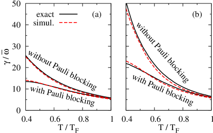
Figure 2: Temperature dependence of the collision rates with (lower curves) and without (upper curves) Pauli blocking for the same system as in Fig. 1. (a) without in-medium effects, (i.e., $\sigma=\sigma_{0}$ and $U=0$); (b) with in-medium cross-section $\sigma_{\text{med}}$ and mean field $U$.

show the collision rates $\gamma$ obtained with the Boltzmann code (dashed lines) and from Eq. (22) (solid lines) as a function of temperature. In order to check the cross section independently from Pauli blocking, we also show the collision rates without Pauli blocking, i.e., the sum of the rates of allowed and blocked collisions [in this case, the exact result is obtained by integrating Eq. (22) without the Pauli-blocking factors $(1-f^{\prime}_{s})$]. Two cases are examined: (a) without medium effects (i.e., with the free cross section $\sigma_{0}$ and without mean field) and (b) with in-medium effects (i.e., with the in-medium cross section $\sigma_{\text{med}}$ and with mean-field $U$). First, we can see on panel (a) that without in-medium effects the collision rates are well reproduced even at low temperature where the Pauli blocking is very important. Looking now at panel (b), we observe that the agreement is still satisfactory in the whole temperature range. Note that the Monte-Carlo integrations have been performed with the exact $\sigma_{\text{med}}$, while in the simulation of course the approximated one (cf. Appendix A) was used. Thus, we can consider that the approximation of $\sigma_{\text{med}}$ is quite accurate and the collision process is well described in the simulation. Finally, the comparison between panels (a) and (b) shows that the in-medium effects significantly increase the collision rate at low temperature, as expected from previous calculations BruunSmith2005 ; Riedl2008 .

IV Comparison with experiments

The aim is now to apply our numerical solution of the Boltzmann equation to realistic cases. We will compare our results with different expansion and collective-mode experiments by the Duke and Innsbruck groups.

IV.1 Anisotropic expansion

The expansion of the gas from an anisotropic trap was shown to be a useful tool to distinguish the collisionless (weakly interacting) case from the hydrodynamic (strongly interacting) one OHara2002 ; Menotti2002 ; Pedri2003 . Recently, more refined analyses of the anisotropic expansion based on viscous hydrodynamics Schaefer2010 were used to extract the temperature dependence of the shear viscosity $\eta$ of the unitary Fermi gas from the experimental expansion data Cao2011 ; Elliott2014a ; Elliott2014b ; Joseph2014 . However, a problem of these analyses is that near the surface of the cloud, the gas is always in the collisionless regime, in which the concept of viscous hydrodynamics is not applicable. It is therefore important to analyse these experiments within the Boltzmann framework, which is capable of describing the hydrodynamic expansion in the center of the cloud and the ballistic expansion of the dilute outer region.

Here, we simulate four expansion experiments of Fermi gases in the unitary limit whose parameters are listed in Table 3.

Table 3: Parameters of the anisotropic expansion experiments of Refs. Cao2011 ; Elliott2014a .

Ref.		Elliott2014a	Cao2011	Cao2011	Cao2011
$\omega_{x}/2\pi$	(Hz)	2210	5283	5283	5283
$\omega_{y}/2\pi$	(Hz)	830	2052	5052	5052
$\omega_{z}/2\pi$	(Hz)	64.3	182.7	182.7	182.7
$\omega_{\text{mag}}/2\pi$	(Hz)	21.5	21.5	21.5	21.5
$N$		$2.5\cdot 10^{5}$	$4\cdot 10^{5}$	$5\cdot 10^{5}$	$6\cdot 10^{5}$
$\tilde{E}/E_{F}$		$1.46$	$2.3$	$3.3$	$4.6$
$T/T_{F}$		$0.51$	$0.79$	$1.11$	$1.54$

The quantity $\tilde{E}$ used by the Duke group to characterize the temperature of the cloud (before the expansion) is twice the potential energy per particle. We transform $\tilde{E}$ into temperature $T$ by calculating $\tilde{E}$ with our equilibrium density profile including the mean field $U$. The system is initialized with the given parameters in the anisotropic trap, then the trap potential is switched off except for the weak magnetic potential $V_{\text{mag}}=\tfrac{1}{2}m\omega_{\text{mag}}^{2}(y^{2}+z^{2}-2x^{2})$ which was present in the experiments during the expansion and which affects merely the expansion in $z$ direction.

In the upper row of Fig. 3

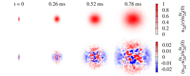
Figure 3: Simulation of the expansion experiment by Elliott et al. Elliott2014a with $\tilde{E}/E_{F}=1.46$. The upper row shows the column density $n_{2d}$ (i.e., the density integrated over $z$) in the $xy$ plane ($x$ in horizontal and $y$ in vertical direction) for different times $t$ after the beginning of the expansion. The lower row shows the error of the fit of the density profile with a Gaussian (see text).

we display the column density $n_{2d}(x,y)=\int dz\,n(x,y,z)$ in the $xy$ plane at different times $t$ after the beginning of the expansion, for initial conditions corresponding to the experiment of LABEL:Elliott2014a with $\tilde{E}/E_{F}=1.46$. One can clearly see the inversion of the aspect ratio during the expansion. To quantify this, we apply the same procedure as in the analysis of the experiment Elliott2014a and determine the cloud widths $\sigma_{x}$ and $\sigma_{y}$ by fitting the density profile with a Gaussian

$$n_{2d}^{\text{fit}}(x,y)\propto e^{-x^{2}/\sigma_{x}^{2}-y^{2}/\sigma_{y}^{2}}\,.$$ (23)

The error of this fit is shown in the lower row of Fig. 3, it does not exceed $2.5\%$ of the central density. In the center, one sees the numerical noise coming from the finite number of test particles ($10^{5}$) used in the simulation. However, in the peripheral regions, where the density is low, we see systematic deviations: in $x$ direction, the cloud is smaller and in $y$ direction it is larger than the fitted Gaussian. This indicates that the expansion does not exactly follow a scaling law of the form $n(r,y,z)=n_{0}(x/b_{x},y/b_{y},z/b_{z})/b_{x}b_{y}b_{z}$ as assumed in previous analyses Schaefer2010 ; Cao2011 ; Elliott2014a ; Elliott2014b ; Joseph2014 . This is not very surprising since one would expect that at the beginning of the expansion, the central part of the cloud follows viscous hydrodynamics and becomes ballistic at later times, while the dilute peripheral part of the cloud expands ballistically from the beginning.

The time dependence of the aspect ratio of the expanding cloud, i.e., the ratio of the fitted cloud widths $\sigma_{x}/\sigma_{y}$, is displayed in Fig. 4

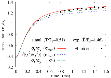
Figure 4: Time dependence of the aspect ratio $\sigma_{x}/\sigma_{y}$ of the expanding cloud in the simulation of the experiment by Elliott et al. Elliott2014a with $\tilde{E}/E_{F}=1.46$.

as the solid line. Our result agrees very well with the experimental data. For comparison, we also show as the dashed line what one obtains if one defines the aspect ratio as $\sqrt{\langle x^{2}\rangle/\langle y^{2}\rangle}$. The discrepancy between the two curves comes from the ballistic low-density part discussed above.

We also studied the influence of the in-medium effects on the expansion. Apparently the effects of mean field and in-medium cross section practically cancel each other if the simulations with and without in-medium effects are made with the same initial temperature $T/T_{F}$. However, the mean field is necessary to get the correct relation between the experimental observable $\tilde{E}/E_{F}$ and the temperature $T/T_{F}$. The dash-dot line in Fig. 4 represents the result for the aspect ratio obtained with mean field but without in-medium effects in the cross section. Since the collision rate with the free cross section $\sigma_{0}$ is lower than the one with the in-medium cross section $\sigma_{\text{med}}$, the inversion of the aspect ratio is somewhat weaker than the one obtained in the full calculation. However, the difference is too small to make a conclusive statement whether the result with or without in-medium cross section is in better agreement with the experimental data.

In Fig. 5

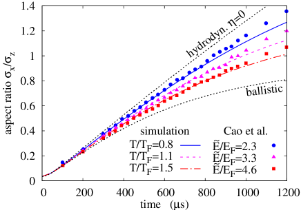
Figure 5: Time dependence of the aspect ratio $\sigma_{x}/\sigma_{z}$ of the expanding cloud in the simulation of the experiments by Cao et al. Cao2011 with $\tilde{E}/E_{F}=2.3$, $3.3$, and $4.6$.

we show results for the aspect ratios in simulations (with mean field and in-medium cross section) starting from a different initial geometry and higher temperatures Cao2011 . For comparison, the dotted lines show the limiting cases of an ideal hydrodynamic ($\eta=0$) and a purely ballistic expansion. One observes that with increasing temperature, the behavior of the system becomes less hydrodynamic and approaches the collisionless regime. The same behavior is seen in the experimental data. Although the agreement between simulation and experiment is not as good as in the case $\tilde{E}/E_{F}=1.46$, it is satisfactory for a theory which does not have any adjustable parameter.

Since in the case of the expansion the calculation is quite simple (one simulation per expansion), we were in this case able to increase the number of test particles and to reduce the time step by factors of two (cf. Table 1). However, already with the smaller number of test particles and the larger time step we obtained practically the same results as shown in Figs. 4 and 5, only in the lower row of Fig. 3 the higher number of test particles shows up in reduced statistical fluctuations around the fitted density profile near the center of the cloud.

IV.2 Quadrupole mode

Let us now study the radial quadrupole oscillation. We consider a trapped gas in the unitary limit with the same characteristics as in the experiment of LABEL:Riedl2008, see Table 2. The quadrupole mode is then excited at $t=0$ by giving all particles a kick

$$p_{x}\to p_{x}+c_{Q}x\,,\qquad p_{y}\to p_{y}-c_{Q}y\,,$$ (24)

(we use $c_{Q}=0.2m\omega_{r}$) and we compute as observable the quadrupole moment

$$Q(t)=\langle x^{2}-y^{2}\rangle(t)\,.$$ (25)

To extract the frequency $\omega_{\mathrm{Q}}$ and damping rate $\Gamma_{\mathrm{Q}}$ of the quadrupole mode from the response $Q(t)$, we fit it with a function of the form

$$Q_{{\text{fit}}}(t)=Ae^{-\Gamma_{\mathrm{Q}}t}\sin\omega_{\mathrm{Q}}t+B(e^{-\Gamma_{\mathrm{Q}}t}\cos\omega_{\mathrm{Q}}t-e^{-\Gamma_{1}t})\,.$$ (26)

The motivation for the choice of this form, including the non-oscillating exponential with decay constant $\Gamma_{1}$, is two-fold: it is similar to the fit function used in the experimental analysis Altmeyer2007 , and it coincides with the form of the response one obtains analytically within the first-order moment method Lepers2010 .

Figure 6

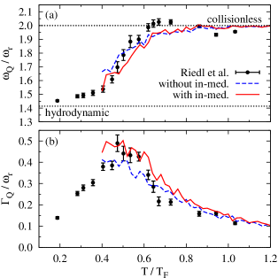
Figure 6: Frequency (a) and damping (b) of the quadrupole mode in a system corresponding to the experiment by Riedl et al. Riedl2008 . In the simulations, we use $1/k_{F}a=-0.1$ instead of the unitary limit to avoid the divergence of the cross section for particles moving in parallel at the same speed. The dotted horizontal lines at $\omega_{\mathrm{Q}}/\omega_{r}=\sqrt{2}$ and $2$ correspond to the frequencies of the quadrupole mode in the hydrodynamic collisionless limits, respectively.

shows the temperature dependence of the frequency (a) and the damping rate (b) of the radial quadrupole mode of the gas whose parameters are given in Table 2. Results obtained with and without in-medium effects ($\sigma_{\text{med}}$, $U$) are shown as solid and dashed lines, respectively. The data points are the experimental results from LABEL:Riedl2008. The irregularities of our results give an idea of the numerical error. Because of the finite number of test particles, the results for $Q(t)$ are somewhat noisy, especially at large times when the amplitude of the mode has strongly decreased. This leads to some uncertainties in the fitted values of $\omega_{\mathrm{Q}}$ and $\Gamma_{\mathrm{Q}}$. Our calculations are globally in good agreement with the data.

The influence of the in-medium effects is surprisingly weak. This is in contrast with Riedl2008 ; Chiacchiera2009 where it was found within the second-order moments method that with in-medium effects, the collisionless regime was reached at too high temperature. Later it was shown that compared with a numerical solution of the Boltzmann equation, the second-order moments method tends to overestimate the collision effects Lepers2010 , and that by extending the moments method to fourth order the discrepancy between the results with in-medium cross section and the experimental data was somewhat reduced Chiacchiera2011 . If one assumes that the moments method converges to the full solution of the Boltzmann equation, the present results suggest that even higher orders in the moments method would further reduce the influence of the in-medium modification of the cross section.

However, we see that at $T/T_{F}\sim 0.4$, the in-medium effects lead to a somewhat lower frequency, which is closer to the data and to the hydrodynamic result $\omega_{\mathrm{Q}}/\omega_{r}\to\sqrt{2}$. Furthermore, the maximum damping near $T/T_{F}=0.5$ is stronger and in better agreement with the data if in-medium effects are included. Unfortunately, the mean field $U$ cannot explain the experimental frequencies $\omega_{\mathrm{Q}}/\omega_{r}>2$ around $T/T_{F}=0.7$, although an attractive mean field is able to increase the frequency of the quadrupole mode in the collisionless limit to values above $2\omega_{r}$ Menotti2002 ; Massignan2005 ; Chiacchiera2009 .

Since our numerical solution of the Boltzmann equation has the necessary flexibility, we can go a step further in our analysis and simulate more closely the experimental procedure. To that end, we excite the mode as before and let the system oscillate for some time $t_{\text{osc}}$, then we switch the trap off and let the system expand during $t_{\text{tof}}=6/\bar{\omega}\approx 2$ ms Altmeyer2007 . Then we calculate the quadrupole moment after the expansion, $Q(t_{\text{osc}}+t_{\text{tof}})$. We repeat the procedure for 50 different values of $\bar{\omega}t_{\text{osc}}$ from $0.04$ to $2.98$ (corresponding to $t_{\text{osc}}\approx 0\dots 1$ ms). Therefore, the whole calculation is very time consuming.

Examples for the quadrupole moment after expansion as a function of $t_{\text{osc}}$ are shown in Fig. 7

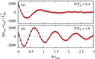
Figure 7: Quadrupole moment after oscillation during $t_{\text{osc}}$ and subsequent expansion during $t_{\text{tof}}=6/\bar{\omega}$, for two different initial temperatures $T/T_{F}=0.4$ (a) and $1.0$ (b). The circles show the results of the simulation with in-medium effects, while the solid line corresponds to the fit by Eq. (27). The system parameters are the same as in Fig. 6.

(circles) for two different initial temperatures. In contrast to the case without expansion Lepers2010 , we see that $Q$ does not vanish for $t_{\text{osc}}=0$. The reason is easy to understand: The excitation by the kick (24) does not immediately create a quadrupole moment, but a quadrupolar velocity field. During the expansion, this is transformed into a quadrupole moment. Therefore, if we want to determine the frequency $\omega_{\mathrm{Q}}$ and damping $\Gamma_{\mathrm{Q}}$, we have to modify the fit function and use instead of Eq. (26) the more general form Altmeyer2007

$$Q_{{\text{fit}}}(t)=Ae^{-\Gamma_{\mathrm{Q}}t}\sin(\omega_{\mathrm{Q}}t+\phi)+Be^{-\Gamma_{1}t}\,.$$ (27)

The fitted functions are also shown in Fig. 7. One can see that, because of the strong damping, the response for $T/T_{F}=0.4$ (a) shows only a single oscillation and is dominated by numerical noise for $t_{\text{osc}}/\bar{\omega}\gtrsim 1.5$. The determination of $\omega_{\mathrm{Q}}$ and $\Gamma_{\mathrm{Q}}$ by the fit with Eq. (27) is thus not very precise in this case (as mentioned before, the same problem limits also the precision of $\omega_{\mathrm{Q}}$ and $\Gamma_{\mathrm{Q}}$ in the case without expansion). At $T/T_{F}=1$ (b), the damping is weaker, and we get a higher precision.

We repeat this procedure for a couple of temperatures. The results for $\omega_{\mathrm{Q}}$ and $\Gamma_{\mathrm{Q}}$ are displayed as the squares in Fig. 8.

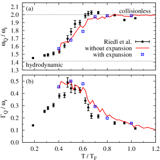
Figure 8: Same as Fig. 6, but the results were obtained from the quadrupole moment with (squares) and without (solid lines) expansion (both include in-medium effects).

Comparing these results with those obtained without expansion (solid lines), one concludes that the expansion before the measurement of the quadrupole moment does not affect the extracted frequencies and damping rates. There is one temperature where some discrepancy is visible, namely $T/T_{F}=0.6$, but as discussed before, the precise extraction of the values $\omega_{\mathrm{Q}}$ and $\Gamma_{\mathrm{Q}}$ is difficult in this region of strong damping.

V Conclusions

In this paper, we described an extension of the test-particle method of LABEL:Lepers2010 for the numerical solution of the Boltzmann equation for ultracold trapped Fermi gases in the normal phase. The main improvements are the possibility to treat realistic particle numbers in realistic (strongly elongated) trap geometries and the inclusion of the mean field and of the in-medium-modifications of the cross section, calculated within a T matrix approximation. This method allows us to simulate several recent experiments on the non-equilibrium dynamics of unpolarized Fermi gases in the normal-fluid phase.

As a first example, we studied the anisotropic expansion of a unitary Fermi gas as measured in Refs. Cao2011 ; Elliott2014a for temperatures $T/T_{F}\geq 0.4$. Without any adjustable parameter, we obtain an excellent agreement with the time dependence of the aspect ratio measured in LABEL:Elliott2014a and an overall reasonable agreement with the data of LABEL:Cao2011. We notice that the peripheral region of the cloud is never hydrodynamic and does not follow the scaling law which approximately describes the expansion.

Then we discussed the radial quadrupole mode as measured in LABEL:Riedl2008. Again, we find that the numerical solution of the Boltzmann equation gives a reasonably good description of the data. In particular, the influence of in-medium effects on the frequency and damping rate of the quadrupole mode seems to be much weaker than in approximate solutions of the Boltzmann equation based on the method of phase-space moments, where it was found to deteriorate the agreement with the data Riedl2008 ; Chiacchiera2009 . We also show that the expansion before the measurement of the deformation of the cloud does not affect the final results for frequency and damping.

These examples show that, if solved correctly, the Boltzmann equation is able to describe out-of equilibrium processes of unpolarized Fermi gases, even in the strongly interacting regime (unitary limit), at a quantitative level, at least at not too low temperatures. Note that even at $T/T_{F}=0.4$, only in a very small part of the trapped gas the temperature is close to the local $T_{c}$ where one would expect pseudogap effects to invalidate the Boltzmann equation. Of course, the Boltzmann equation is not applicable below the superfluid transition temperature ($\sim 0.3\,T_{F}$ for a trapped gas).

Since our Boltzmann code reproduces the anistroptic expansion experiments of Refs. Cao2011 ; Elliott2014a , it would be interesting to adapt it to calculate directly the temperature dependence of the shear viscosity $\eta$, and to compare it with the one extracted from the experiments under relatively strong assumptions (a refined analysis was made in LABEL:Joseph2014). In principle, the result should be similar to that of Refs. BruunSmith2005 ; BluhmSchaefer2014 , where the viscosity was also calculated from the Boltzmann equation with in-medium effects.

A challenging subject for future work would be the description of shock waves as studied experimentally in Joseph2011 by splitting the initial cloud into two and letting them collide in $z$ direction. The difficulty of this problem compared to the phenomena studied in the present work is the rapid change of the distribution function on a short length scale in the direction of the long axis of the trap.

Also a quantitative description of the collision of two spin-polarized clouds with opposite polarization as in the experiment of LABEL:Sommer2011 is still missing. On a qualitative level, it was already shown in LABEL:Goulko2011 that the Boltzmann equation without in-medium effects can reproduce the different regimes (bounce, transmission) that were experimentally observed. What is particularly difficult in this case is the inclusion of in-medium effects, since the T matrix approximation used in the present work fails in the polarized case. A step into this direction was undertaken in LABEL:Pantel2014.

Appendix A Approximations for the in-medium cross section

Depending on the temperature, we use two different strategies to approximate the in-medium cross section.

A.1 Low temperature

At low temperature, $\sigma_{\text{med}}$ has typically a peak near $q=k_{F}$ (where $k_{F}$ is the Fermi momentum), especially for small total momenta $k$ (cf. Fig. 2 in LABEL:Chiacchiera2009). At very large $k$ or $q$, it approaches the free cross section $\sigma_{0}$. One might therefore try to fit Eq. (17) with a function of the form

$$\sigma_{\text{fit}}(k,q)=\sigma_{0}(q)\left[1+Ae^{-k^{2}/k_{0}^{2}}\frac{1}{(q-q_{0})^{2}+q_{1}^{2}}\right],$$ (28)

where the parameters $A,k_{0},q_{0}$, and $q_{1}$ are functions depending on $T$, $\bar{\mu}$ and $a$ to be determined (as mentioned above, we consider only the unpolarized case, i.e., $\mu_{\uparrow}=\mu_{\downarrow}=\bar{\mu}$). However, the problem with a fit is that it is not clear how the different $k$ and $q$ should be weighted; furthermore, the obtained parameters $A,\dots,q_{1}$ as functions of $T$, $\bar{\mu}$ and $a$ are too noisy to be interpolated.

We therefore follow a slightly different strategy. As a measure for the quality of the parameterization, one can take its capability to reproduce certain physical properties that depend on the cross-section. For instance, one wishes to reproduce the equilibrium values of the collision rate per particle, $\gamma$, or of the viscous relaxation time, $\tau$.

Thus, instead of fitting directly $\sigma_{\text{med}}$ with $\sigma_{\text{fit}}$, we determine the four parameters of $\sigma_{\text{fit}}$ such as to reproduce four different moments (i.e., integrals weighted with different powers of $k$ and $q$) of $\sigma_{\text{med}}$,

$$m^{\text{med}}_{j}=\int dk\int dq\sigma_{\text{med}}(k,q)\kappa(k,q)\phi_{j}(k,q)\,,$$ (29)

where $\kappa$ reads

$$\kappa(k,q)=\left[\frac{\operatorname{atanh}\left(\tanh\frac{X}{2}\tanh\frac{Y}{2}\right)}{\sinh X}\right]^{2},$$ (30)

with $X=2\beta\omega$ and $Y=\beta kq/2m$, and the four weight functions $\phi_{j}$ ($j\in\{1,\dots,4\}$) are

$$\phi_{1}=q\,,\quad\phi_{2}=q^{3}\,,\quad\phi_{3}=q^{5}\,,\quad\phi_{4}=k^{2}q^{3}\,.$$ (31)

The four parameters $A\dots q_{1}$ are now determined from the four equations $m^{\text{med}}_{j}=m^{\text{fit}}_{j}$ (the $m^{\text{fit}}_{j}$ have of course the same expressions as $m^{\text{med}}_{j}$, only the cross section has to be changed accordingly). Since $m^{\text{med}}_{1}$ is exactly related to $\gamma$ [cf. Eq. (22)], and $m^{\text{med}}_{4}$ is similar to the integral appearing in the calculation of $\tau$ (cf. LABEL:Chiacchiera2009), we are sure that $\sigma_{\text{fit}}$ will give good results for $\gamma$ and $\tau$.

A.2 High temperature

When the temperature increases, the shape of $\sigma_{\text{med}}$ becomes flatter and the Lorentzian part of $\sigma_{\text{fit}}$ does not fit the real behavior any more. At high temperature, the chemical potential becomes negative and the Fermi functions in Eq. (19) can be expanded as $f_{0}(\xi)=e^{-\beta\xi}-e^{-2\beta\xi}+e^{-3\beta\xi}-\dots$. As a consequence, the expansion of $J$ reads

$$J(\omega,\bm{\mathrm{k}};T)\approx J_{\text{ht}}(\omega,\bm{\mathrm{k}};T)-J_{\text{ht}}(\omega,\bm{\mathrm{k}};T/2)\\ +J_{\text{ht}}(\omega,\bm{\mathrm{k}};T/3)-\dots\,.$$ (32)

The result for high-temperature limit $J_{\text{ht}}$ can be written in closed form as

$$J_{\text{ht}}(\omega,\bm{\mathrm{k}};T)=\frac{m^{2}e^{\beta\bar{\mu}}}{2\pi\beta k}\Bigl{[}\frac{2}{\sqrt{\pi}}[F(X_{+})-F(X_{-})]\\ +i\left(e^{-X_{-}^{2}}-e^{-X_{+}^{2}}\right)\Bigr{]},$$ (33)

where $X_{\pm}=(q\pm k/2)/\sqrt{2mT}$ and $F$ denotes Dawson’s integral AbramowitzStegun (see Appendix B).

In practice, we use the first three terms of the high-temperature expansion in the case $\bar{\mu}<0$, and the parameterization $\sigma_{\text{fit}}$ otherwise.

Appendix B Approximation for Dawson’s integral

In the high-temperature expansion of the in-medium cross section there appears a function $F(x)$, called Dawson’s integral AbramowitzStegun and defined by

$$F(x)=e^{-x^{2}}\int_{0}^{x}e^{t^{2}}dt\,.$$ (34)

Since speed is more important than precision for our purpose, we approximate $F(x)$ for $-\infty<x<\infty$ by a simple rational function of the form

$$F(x)\approx\frac{x+a_{1}x^{3}+a_{2}x^{5}}{1+b_{1}x^{2}+b_{2}x^{4}+2a_{2}x^{6}}\,,$$ (35)

which automatically reproduces the asymptotic behavior of $F(x)$ for $x\to 0$ and $x\to\pm\infty$. By minimizing the maximum relative error, we obtain the following values for the parameters:

$$a_{1} =0.133931\,, b_{1} =0.853463\,,$$

$$a_{2} =0.0989404\,, b_{2} =0.228679\,.$$ (36)

The maximum relative error of this approximation is $0.53\%$.

References

- (1) M. J. Wright, S. Riedl, A. Altmeyer, C. Kohstall, E. R. Sánchez Guajardo, J. Hecker Denschlag, and R. Grimm, Phys. Rev. Lett. 99, 150403 (2007).
- (2) S. Riedl, E. R. Sanchez Guajardo, C. Kohstall, A. Altmeyer, M. J. Wright, J. H. Denschlag, R. Grimm, G. M. Bruun, and H. Smith, Phys. Rev. A 78, 053609 (2008).
- (3) K. M. O’Hara, S. L. Hemmer, M. E. Gehm, S. R. Granade, and J. E. Thomas, Science 298, 2179 (2002).
- (4) C. Menotti, P. Pedri, and S. Stringari, Phys. Rev. Lett. 89, 250402 (2002).
- (5) P. Pedri, D. Guéry-Odelin, and S. Stringari, Phys. Rev. A 68, 043608 (2003).
- (6) T. Schäfer, Phys. Rev. A 82, 063629 (2010).
- (7) C. Cao, E. Elliott, J. Joseph, H. Wu, J. Petricka, T. Schäfer, and J. E. Thomas, Science 331 58 (2011),
- (8) E. Elliott, J. A. Joseph, and J. E. Thomas, Phys. Rev. Lett. 112, 040405 (2014).
- (9) E. Elliott, J. A. Joseph, and J. E. Thomas, Phys. Rev. Lett. 113, 020406 (2014).
- (10) J. A. Joseph, E. Elliott, and J. E. Thomas, arXiv:1410.4835 (2014).
- (11) T. Schäfer and D. Teaney, Rept. Prog. Phys. 72, 126001 (2009).
- (12) F. Toschi, P. Vignolo, S. Succi, and M. P. Tosi, Phys. Rev. A 67, 041605 (2003).
- (13) P. Massignan, G. M. Bruun, and H. Smith, Phys. Rev. A 71, 033607 (2005).
- (14) G. M. Bruun and H. Smith, Phys. Rev. A 76, 045602 (2007).
- (15) S. Chiacchiera, T. Lepers, D. Davesne, and M. Urban, Phys. Rev. A 79, 033613 (2009).
- (16) T. Lepers, D. Davesne, S. Chiacchiera, and M. Urban, Phys. Rev. A 82, 023609 (2010).
- (17) S. Chiacchiera, T. Lepers, D. Davesne, and M. Urban, Phys. Rev. A 84, 043634 (2011).
- (18) Lei Wu and Yonghao Zhang, Europhys. Lett. 97, 16003 (2012)
- (19) G. F. Bertsch and S. Das Gupta, Phys. Rep. 160, 189-233 (1988).
- (20) F. Toschi, P. Capuzzi, S. Succi, P. Vignolo, and M. P. Tosi, J. Phys. B 37, S91 (2004).
- (21) A. C. J. Wade, D. Baillie, and P. B. Blakie, Phys. Rev. A 84, 023612 (2011).
- (22) O. Goulko, F. Chevy, and C. Lobo, Phys. Rev. A 84, 051605(R) (2011).
- (23) O. Goulko, F. Chevy, and C. Lobo, New J. Phys. 14, 073036 (2012).
- (24) P.-A. Pantel, D. Davesne, S. Chiacchiera, and M. Urban, Phys. Rev. A 86, 023635 (2012).
- (25) G. M. Bruun and H. Smith, Phys. Rev. A 72 043605 (2005).
- (26) M. Bluhm and T. Schäfer, arXiv:1410.2827 [cond-mat.quant-gas] (2014).
- (27) M. Urban, Phys. Rev. C 85, 034322 (2012)
- (28) W. Kohn, Phys. Rev. 123, 1242 (1961).
- (29) A. Altmeyer, S. Riedl, M. J. Wright, C. Kohstall, J. H. Denschlag, and R. Grimm, Phys. Rev. A 76, 033610 (2007).
- (30) J. A. Joseph, J. E. Thomas, M. Kulkarni, and A. G. Abanov, Phys. Rev. Lett 106, 150401 (2011).
- (31) A. Sommer, M. Ku, G. Roati, and M. W. Zwierlein, Nature 472, 201 (2011).
- (32) P.-A. Pantel, D. Davesne, and M. Urban, Phys. Rev. A 90, 053629 (2014).
- (33) M. Abramowitz and I. A. Stegun (eds.), Handbook of Mathematical Functions (Dover, New York, 1965).