Slowing down of vortex motion in thin NbN films
near the superconductor-insulator transition

Abstract

We present a quantitative comparison between the measurements of the complex conductance at low (kHz) and high (GHz) frequency in a thin superconducting film of NbN and the theoretical predictions of the dynamical Beresinksii-Kosterlitz-Thouless theory. While the data in the GHz regime can be well reproduced by extending the standard approach to the realistic case of a inhomogeneous sample, the low-frequency measurements present an anomalously large dissipative response around $T_{c}$. This anomaly can only be accounted for by assuming a strong slowing down of the vortex diffusion in the kHz regime, or analogously a strong reduction of the length scale probed by the incoming finite-frequency field. This effect suggests the emergence of an intrinsic length scale for the vortex motion that coincides with the typical size of inhomogeneity probed by STM measurements in disordered NbN films.

I Introduction

More than forty years after its discovery,review_minnaghen ; jose_book the Beresinksii-Kosterlitz-Thouless (BKT) transitionbkt ; bkt2 still represents one of the most fascinating phenomena in condensed-matter systems. Indeed, it describes the universality class for the phase transition in two spatial dimensions in a system displaying $U(1)$ symmetry. After its original formulation within the classical $XY$ spin model, it has been later on applied to a wide class of phenomena, mostly related to the superfluid or superconducting (SC) transition in two dimensions, as it occurs in artificial Josephson junctions, thin films, and recently also cold atoms.jose_book In all these cases the transition is driven by topological vortex excitations instead of the usual vanishing of the order parameter, leading to striking predictions for the behaviour of several physical quantities.

The most famous hallmark of BKT physics is certainly the discontinuous but universal jump of the density of superfluid carriers at the transition,nelson_prl77 that has been successfully observed in superfluid He films.helium4 However in the case of superconducting materials the superfluid-density jump turned out to be rather elusive: indeed, while some signatures have been identified in thin films of conventional superconductors as MoGeMoGe ; yazdani_prl13 , InOxfiory_prb83 ; armitage_prb07 ; armitage_prb11 and NbN,kamlapure_apl10 ; mondal_bkt_prl11 ; yong_prb13 they are less evident in other cases as thin films of high-temperature cuprate superconductorslemberger_prb12 or SC interfaces between oxides.moler_prb12 The lack of clear BKT signatures is due in part to two intrinsic characteristics of the SC films, absent in superfluid ones:review_minnaghen (i) the presence of quasiparticle excitations, that contribute to the decrease of the superfluid density limiting the observation of BKT effects to a small temperature range between $T_{BKT}$ and the BCS critical temperature $T_{c}$, and (ii) the screening effects due to charged supercurrents. The latter can be avoided by decreasing the film thickness $d$, so that the Pearl lengthreview_minnaghen $\Lambda=2\lambda^{2}/d$, where $\lambda$ is the penetration depth, exceeds the sample size making the interaction between vortices effectively long-ranged. However, this also implies that in the case of conventional superconductors, like InOx and NbN, the observation of BKT physics is restricted to samples near to the superconductor-to-insulator transition (SIT), where several additional features must be considered along with the presence of BKT vortices. The most important one is the emergence at strong disorder of an intrinsic inhomogeneity of the SC properties, as shown in the last few years by detailed tunneling spectroscopy measurements.sacepe_11 ; mondal_prl11 ; pratap_13 ; noat_prb13

Such intrinsic granularity of disordered SC films, that has been interpreted theoretically as the compromise between charge localization and pair hopping near the SIT,ioffe ; nandini_natphys11 ; seibold_prl12 ; lemarie_prb13 has been efficiently incorporated in the BKT description of the superfluid density as an average of the superfluid response over the distribution of local critical temperatures.benfatto_prb08 ; review13 This leads to a drastic smearing of the superfluid-density jump predicted by the conventional BKT theory, in accordance with the experimental observations of the inductive response in thin films of conventional superconductors,mondal_bkt_prl11 ; yong_prb13 as measured by means of two-coil experiments. Notice that this experimental set-up measures the complex conductivity $\sigma(\omega)$ of a superconductor at low but finite frequency $\omega$, usually $\omega\simeq 50-60$ kHz. As a consequence, along with the superfluid response, connected to the imaginary part $\sigma_{2}(\omega)$, it also allows one to measure the dissipative part $\sigma_{1}(\omega)$, that displays a peak slightly above $T_{BKT}$, whose width in temperature correlates usually with the broadening of the superfluid-density jump.yong_prb13

According to the standard viewambegaokar_prb80 ; HN the largest contribution to $\sigma_{1}(\omega)$ near $T_{BKT}$ is expected to come from the same vortex excitations that control the suppression of the superfluid density. Indeed, the finite dissipation comes essentially from the cores of the vortices thermally excited above $T_{BKT}$, that can move at finite probing frequency over a length scale $r_{\omega}$ of the order of $r_{\omega}\simeq\sqrt{D/\omega}$. Here $D$ is the vortex diffusion constant, that is usually assumedambegaokar_prb80 to coincide with the electron diffusion constant. The maximum of $\sigma_{1}$ is then expected to occur at the temperature $\bar{T}$ above $T_{BKT}$ where $\xi(\bar{T})\simeq r_{\omega}$, where $\xi(T)$ is the BKT correlation length. As a consequence, one would expect a shift or the $\sigma_{1}$ maximum towards higher temperatures, along with a broadening and enhancement of the dissipative peak as $\omega$ increases. As we will show in this paper, these conditions are strongly violated in thin films of disordered NbN. By comparing the experimental results obtained on the same sample measured both at low (10 to 100 kHz) and high (1 to 10 GHz) frequency we show that the dissipative response is approximately the same in the two regimes. When compared with the theoretical predictions for the BKT transition in an inhomogeneous system these results imply that the dissipation observed in the kHz regime is anomalously large, as reported before also MoGe and InO films,MoGe while in the GHz regime the observed resistive contribution agrees approximately with the BKT expectation. Within our approach the large resistive contribution observed in the kHz range can be accounted for only by assuming a strong reduction of the vortex difussion constant with respect to the conventional value of the Bardeen-Stephen theory. Such a slowing down of vortices at low frequency can be also rephrased as the emergence of an intrinsic length scale cut-off $\xi_{V}$ for vortex diffusion in our disordered thin films, that makes the dissipative response quantitatively very similar in the two range of frequencies. More importantly, $\xi_{V}$ correlates well with the typical size of SC islands observed in similar samples by STM,mondal_prl11 ; pratap_13 showing that the disorder-induced inhomogeneity is a crucial and unavoidable ingredient to understand the occurrence of BKT physics in thin films.

The plan of the paper is the following. In Sec. II we present the experimental results obtained by means of two-coils mutual inductance technique in the kHz and by means of measurements in the Corbino geometry in the microwave. The direct comparison between the experimental data obtained on the same sample in the two regimes of frequencies shows clearly the emergence of an anomalously large dissipative response at low frequency. To quantify this anomaly we introduce in Sec. III the standard BKT approach for the finite-frequency response in a homogeneous system, and show its failure to reproduce the experimental data. In Sec. III we extend the finite-frequency BKT approach to include the effect of inhomogeneity, along the line of previous work done in the static case.mondal_bkt_prl11 ; review13 ; yong_prb13 . Within this scheme we discuss the role played by the anomalous vortex diffusion constant at low frequency, and we comment on its relation to real-space structures due to disorder. The final remarks are presented in Sec. V. Finally, Appendix A contains some additional technical detail on the description of the BKT physics at finite frequency.

II Experimental results

II.1 Details of the measurements and analysis

The electrodynamic response was studied on a 3 nm thick NbN sample, that we expect to be in the 2D limit as previous measurements in analogous samples have shown.mondal_bkt_prl11 The superconducting BKT transition was studied in both kHz(10 to 100 kHz) and microwave(1 GHz to 10 GHz) frequency range on the same sample to explore vortex diffusion as a function of the probing length scale.

The kHz data were acquired using a home-built two-coil mutual inductance set-up,kamlapure_apl10 where we drive the primary coil at a desired frequency varying from 10-100 kHz. The amplitude of ac excitation is kept at 10 mOe. The sample here is a circle of diameter of 8 mm, which we prepare by DC magnetron sputtering of Nb on MgO(100) in an argon-nitrogen gas mixture. We place the sample in between the coaxial primary and secondary coil, and we measure the induced voltage of the secondary coil. Since the degree of coupling between the coils varies with temperature due to the variation of complex penetration depth $\lambda_{\omega}$ ( $\lambda_{\omega}=(\lambda^{-2}+i\delta^{-2})^{-1/2}$, see Eqs. (10)-(11) below) of the superconducting film, the real and imaginary part of the voltage induced in the secondary coil gives the complex mutual inductance $M_{exp}$ of the coils as a function of temperature. The theoretical value of $M_{theo}$ as a function of $\lambda_{w}$ can be determined by solving numerically the coupled set of Maxwell and London equations for the particular coil and sample geometry of our set-up. The numerical method takes into account the effect of the finite radius of the film, as proposed by J. Turneaure,Turneaure1 ; Turneaure2 see also Ref. [mintuthesis, ]. We obtain a 2D matrix (typically 100 $\times$ 100) of complex mutual inductance values for different sets of Re($\lambda_{w}^{-2}$) and Im($\lambda_{w}^{-2}$). Then we compare $M_{exp}$ with the calculated $M_{theo}$ in order to extract $\lambda_{w}$ as a function of temperature.

Microwave spectroscopy was carried out in Corbino geometrymondal_scire13 on the same piece of sample after cutting it in 5 mm $\times$ 5 mm size and thermally evaporating Ag on it. By using the same piece of the sample we can avoid any effect of change in the SC properties (SC gap, superfluid stiffness, etc.) while studying two different frequency regimes. In this way we can attribute the change of the optical response only to variations of the vortex diffusion constant, which is the aim of the present work. The sample here terminates a 1 m long ss coaxial cable to reflect the microwave signal, generated internally from a vector network analyser (VNA) spanning 10 MHz to 20 GHz. The complex reflection coefficient($S_{11}$) measured by the VNA is first corrected using three error coefficients for the cable, which we get after calibration with three standards.ohashi ; dressel ; booth To calibrate the cable at experimental condition, i.e at low temperature, we use as short standard the spectrum of a thick ordered NbN sample taken at the lowest temperature, and as loads the sample spectra taken at two different temperatures above $T_{c}$. Such a calibration technique is less prone to error, since two of the three calibrators are measured during the same thermal cycle with the actual sample. The corrected $S_{11}$ is then related to the complex impedance $Z$ of the sample by means of the relation:

$$S_{11}=\frac{(Z-Z_{0})}{(Z+Z_{0})}$$ (1)

where $Z_{0}$ is the characteristic impedance of the cable, i.e. 50 $\Omega$ in our case. The complex conductivity $\sigma$ of the sample is the given by

$$\sigma=\frac{\ln(b/a)}{2\pi dZ}$$ (2)

where $a$ and $b$ are the inner and outer radius of the film, and $d$ is the thickness.

II.2 Experimental data

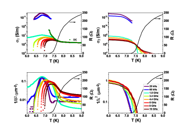
Figure 1: (Color online) Experimental data of $\sigma_{1}$ and $\sigma_{2}$ at both kHz and GHz frequency range(panel (a) and (b)).Panel (c) and (d) show the comparison of $\delta^{-2}$ and $\lambda^{-2}$ at similar frequencies. The panels contain also the result of simultaneous dc resistance measurement. Notice that $\sigma_{1}$ in the microwave regime matches perfectly above $T_{c}$ the value of the dc conductivity obtained by the measured resistance, see panel (a).

The results of the kHz and GHz measurement of the complex conductivity are shown in Fig. 1a,b. Notice that even though the kHz measurements lose sensitivity away from $T_{c}$, our microwave measurements can capture the normal state conductivity quite well, and it exactly matches the one obtained from dc measurement (see Fig. 1a). To compare data at different frequencies it is more convenient to convert the complex conductivity in a length scale:

$$\lambda^{-2} = \mu_{0}\omega\sigma_{2},$$ (3)

$$\delta^{-2} = \mu_{0}\omega\sigma_{1},$$ (4)

where $\lambda^{-2}$ coincides with the usual SC penetration depth, proportional to the superfluid density of the sample (see Eq. (13) below). At finite frequency $\lambda^{-2}$ persists slightly above $T_{c}$, in a temperature range that increases proportionally to the probing frequency, as observed also in thick samples,mondal_scire13 and as expected by scaling near criticality.ffh This effect, shown in Fig. 1d, is negligible for low frequency and becomes appreciable in the microwave regime. The low-temperature part of $\lambda^{-2}$ can be fitted very well by means of a BCS formula, as shown in Fig. 2. However, near $T_{c}$ a sudden deviation of $\lambda^{-2}$ from the BCS fit occurs, signaling the occurrence of a vortex-induced BKT transition. As already observed before,mondal_bkt_prl11 ; yong_prb13 the low vortex fugacity of NbN films moves the BKT transition at temperatures slightly smaller than the one where the BCS curve intersects the universal BKT line (see also Eq. (13) below).

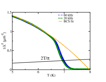
Figure 2: (Color online) Inverse penetration depth at low frequency compared with a BCS fit of the low-temperature part. The deviation from the BCS fit, which occurs slightly before than the intersection with the universal line $2T/\pi$, signals the occurrence of a BKT transition due to thermally excited vortices. The ratio $\Delta(0)/T_{c}=2.2$ obtained from the fit, with $T_{c}$ BCS temperature, agrees well with the estimate given by tunnelling experiments in thick NbN films.mondal_prl11

The length $\delta^{-2}$ is instead a measure of the fluctuations around $T_{c}$, that originate in our BKT sample by the vortex motion at finite frequency, as we shall discuss below. On very general ground, one can associate the probing frequency $\omega$ with a finite length scale $r_{\omega}$ by means of the diffusion coefficient $D$:ambegaokar_prb80

$$r_{\omega}=\sqrt{\frac{14D}{\omega}}.$$ (5)

Within the standard Bardeen-Stephen modelHN the vortex motion causes dissipation because of the normal-electron component present in the vortex cores. Thus, the diffusion constant $D$ in Eq. (5) should scale with the electron diffusion constant, that can be estimated from the Fermi velocity and the mean free path obtained by resistivity and Hall measurements at 285K, as $D\simeq 10^{-5}m^{2}/s$. Thus, in the kHz regime $r_{\omega}$ should approch the system size, giving negligible dissipative effects, in sharp contrast to the experimental observation. Indeed, the intensity of $\delta^{-2}$ and the peak width are similar both in the kHz and the GHz regime, despite a change of frequency by six orders of magnitude, see Fig. 1d and 1c). As we shall discuss in the next section, the anomalously large dissipative response found in the kHz frequency regime is the hallmark that inhomogeneity cut-off the vortex diffusion at scales $r_{\omega}\sim\xi_{V}$ of order of the typical size $\xi_{inh}$ of the inhomogeneous domains. Thus, while in the GHz regime a standard value of the diffusion constant leads to a probing length $r_{\omega}$ that is already of the order of $\xi_{inh}$, leading to a dissipative response in good quantitative agreement with standard predictions for the BKT theory in an inhomogeneous system, in the kHz regime the same approach fails, unless one assumes a diffusion constant $D$ much smaller than what predicted by the Bardeen-Stephen theory.

III Dynamical BKT theory: the conventional view

The extension of the BKT theory to include dynamics effects was developed soon after its discovery in a couple of seminal papers by Ambegaokar et al., ambegaokar_prb80 who considered the case of superfluid Helium, and afterwards by Halperin and Nelson,HN who extended it to charged superconductors. The effect of the transverse motion of vortices under an applied electric field is then encoded in an effective frequency-dependence dielectric function $\varepsilon(\omega)$, in analogy with the motion of the charges for the Coulomb plasma. The resulting complex conductivity of the film can be expressed as:HN ; review_minnaghen

$$\sigma(\omega)=-\frac{n^{0}_{s}de^{2}}{i\omega m\varepsilon(\omega)},$$ (6)

$m$ the electron mass and $n_{s}^{0}$ is the mean-field superfluid density, i.e. the one including BCS quasiparticle excitations but not the effect of vortices. The dielectric function is controlled by the fundamental scaling variables appearing in the BKT theory,review_minnaghen ; review13 i.e. the bare superfluid stiffness $J$ and the vortex fugacity $g$, defined as usual by

$$J=\frac{\hbar^{2}n^{0}_{s}d}{4m},\quad g=2\pi e^{-\beta\mu},$$ (7)

where $\mu$ is the vortex-core energy. As it is well known,bkt2 ; review_minnaghen ; review13 the role of vortices at large distances can be fully captured by the renormalization-group (RG) equations of the BKT theory for the two quantities $g$ and $K\equiv\pi J/T$:

$$\frac{dK}{d\ell} = -K^{2}g^{2},$$ (8)

$$\frac{dg}{d\ell} = (2-K)g,$$ (9)

where $\ell=\ln(a/\xi_{0})$ is the RG-scaled lattice spacing with respect to the coherence length $\xi_{0}$, that controls the vortex sizes and appears as a short-scale cut-off for the theory. From Eq. (6) we can derive the real and imaginary part of the conductivity in terms of the bare stiffness $J$ and the dielectric function, so that one has, in agreement with Eqs. (3)-(4) above:

$$\lambda^{-2} = \mu_{0}\omega\sigma_{2}=\frac{J}{d\alpha}\mathrm{Re}\frac{1}{\varepsilon}=\frac{J}{d\alpha}\frac{\varepsilon_{1}}{\varepsilon_{1}^{2}+\varepsilon_{2}^{2}},$$ (10)

$$\delta^{-2} = \mu_{0}\omega\sigma_{1}=-\frac{J}{d\alpha}\mathrm{Im}\frac{1}{\varepsilon}=\frac{J}{d\alpha}\frac{\varepsilon_{2}}{\varepsilon_{1}^{2}+\varepsilon_{2}^{2}}.$$ (11)

where $\alpha=\hbar^{2}/4e^{2}\mu_{0}$ is a numerical factor. In particular, if $\lambda$ is expressed in $\mu$m, $d$ in Å and $J$ in K, then $\alpha=0.62$. As we discuss in details in Appendix A, $\varepsilon(\omega)$ is a function of both $K$ and $g$. In particular, in the static limit one can show that $\varepsilon$ is purely real, and it is given by:

$$\varepsilon(\omega=0)=\varepsilon_{1}=\frac{K(0)}{K(\ell\rightarrow\infty)}=\frac{J(0)}{J(\ell\rightarrow\infty)},$$ (12)

so that $\delta^{-2}=0$ and the inverse penetration depth $\lambda^{-2}$ is controlled by the renormalized stiffness $J_{s}$ introduced in Refs. [nelson_prl77, ; review13, ]:

$$J_{s}\equiv\frac{TK(\ell=\infty)}{\pi}\equiv\frac{\hbar^{2}n_{s}d}{4m}=\frac{\alpha d}{\lambda^{2}}.$$ (13)

with $n_{s}$ real superfluid density, including also vortex-excitation effects. According to the RG equations (8), when $K\gtrsim 2$ the fugacity $g$ flows to zero at large distances, so that $K(\ell\rightarrow\infty)\neq 0$. The resulting $J_{s}$ is finite but in general smaller than its BCS counterpart $J$, due to the effect of bound vortex-antivortex pairs at short length scales, as it has been discussed in the context of NbN thin films.mondal_bkt_prl11 ; yong_prb13 Instead when $K\lesssim 2$, $g$ diverges, signalling the proliferation of free vortices. The BKT transition temperature is the one where $K(\ell=\infty)=2$, so that at $T_{BKT}$ $J_{s}$ if finite and it jumps discontinuously to zero right above it:

$$J_{s}(T_{BKT}^{-})=\frac{2T_{BKT}}{2},\quad J_{s}(T_{BKT}^{+})=0.$$ (14)

At finite frequency $\varepsilon(\omega)$ develops an imaginary part due to the vortex motion: in first approximation (see also Appendix A) one can putambegaokar_prb80

$$\varepsilon_{2}\simeq\frac{Dn_{f}}{\omega}=\frac{D}{\omega\xi^{2}}\sim\left(\frac{r_{\omega}}{\xi}\right)^{2},$$ (15)

where $n_{f}$ is the free-vortex density, expressed in terms of the vortex correlation length $\xi$, and $r_{\omega}$ is the frequency-dependent probing length scale introduce in Eq. (5) above. The length scale $r_{\omega}$ provides also a cut-off for the real part of the dielectric function, that is given approximately by Eq. (12) with $\ell=\infty$ replaced by $\ell_{\omega}=\ln(r_{\omega}/\xi_{0})$:

$$\varepsilon_{1}(\omega)\simeq\frac{J(0)}{J(\ell_{\omega})},$$ (16)

so that instead of the discontinuous divergence of $\varepsilon_{1}$ expected for $\omega=0$, due to the superfluid-density jump (14), one finds a rapid increase across $T_{BKT}$. The resulting temperature dependence of $\lambda^{-2}$ and $\delta^{-2}$ in Eqs. (10)-(11) is controlled by the increase of $\varepsilon_{1},\varepsilon_{2}$ across $T_{BKT}$. In particular, since $\varepsilon_{2}$ from Eq. (15) becomes sizeable when one moves away from $T_{BKT}$ due to the proliferation of free vortices, until it overcomes $\varepsilon_{1}$, $\lambda^{-2}$ displays a rapid downturn instead of the discontinuous jump (14) of the static theory. Instead $\delta^{-2}$ in Eq. (11) starts to increase at $T_{BKT}$ and shows a maximum at approximately the temperature $\bar{T}$ where $\varepsilon_{2}\simeq\varepsilon_{1}\sim{\cal O}(1)$. In terms of the characteristic length scales appearing in Eq. (15) this occurs when

$$\xi(\bar{T})\approx r_{\omega}.$$ (17)

The correlation length within the BKT theory is described by an exponentially-activated behaviorbkt ; review_minnaghen ; HN ; review13

$$\xi\simeq A\xi_{0}\exp\left(\frac{b}{\sqrt{t}}\right),$$ (18)

where the coefficient $b$ is connected to the distance between the $T_{BKT}$ and the mean-field temperature $T_{c}$, and to the vortex-core energy:HN ; benfatto_prb09

$$b\simeq\frac{4}{\pi^{2}}\frac{\mu}{J}\sqrt{t_{c}},\quad t_{c}={\frac{T_{c}-T_{BKT}}{T_{BKT}}}.$$ (19)

By means of Eq. (18), and using $\mu/J\simeq 1$ as evidenced by the analysis of the $\lambda^{-2}$ far from the transition regime we are investigating,mondal_prl11 we then obtain that up to multiplicative factors of order one the transition width at finite frequency is approximately:

$$\frac{\bar{T}-T_{BKT}}{T_{BKT}}\simeq\frac{1}{[\ln(r_{\omega}/\xi_{0})]^{2}}t_{c}.$$ (20)

The above Eq. (20) confirms the general expectation that the broadening of the transition due to finite-frequency effects is fully controlled by the probing length scale $r_{\omega}$, where the diffusion constant enters in a crucial way, see Eq. (5). Let us then start with an estimate of the finite-frequency effects in NbN based on the standard value of the diffusion constant given by the Bardeen-Stephen model, where $D$ coincides with the diffusion constant of electrons $D_{e}\simeq v_{F}\ell_{loc}$, that is around $D_{e}\simeq 10^{-5}m^{2}/s$ in NbN.mondal_scire13 The distance between $T_{c}$ and $T_{BKT}$ can be estimated by a BCS fit of the data at low temperatures, as shown in Fig. 3a, and it is in the present case $t_{c}=0.1$. Finally, for $\xi_{0}\simeq 10$ nm, as appropriate for NbN,xi0 one obtains from Eq. (17)

$$\bar{T}-T_{BKT}\simeq 0.01K.$$ (21)

This estimate is confirmed by the numerical calculation of the optical response based on the full expression of the dielectric function $\varepsilon(\omega)$ reported in Appendix A, and shown in Fig. 3c,d. As one can see, finite-frequency effects lead indeed to a neglegible smoothening of the superfluid-density jump with respect to the static case, and to a finite dissipative response $\delta^{-2}$ whose width in temperature is two order of magnitude smaller than what observed in real data, reported in Fig. 3b. The result for $\lambda^{-2}$ can be easily understood by comparing the scale $r_{\omega}$ with the other two length scales that act as cut-off on the RG equations (8)-(9) already in the static case, i.e. the system size $R\simeq 8$ mm and the Pearl length $\Lambda=2\lambda^{2}/d$, that at $T_{BKT}$ (where $\lambda^{-2}\simeq 0.5\mu$m^-2) is of the order of $\Lambda\simeq 1$ mm. For a conventional value $D_{e}\simeq 10^{-5}m^{2}/s$ of the diffusion constant $r_{\omega}\simeq 1$ cm at 10 kHz, i.e. it is even larger than both $R$ and $\Lambda$. Thus, the rounding effects at finite frequency on $\lambda^{-2}$ shown in Fig. 3c do not differ considerably from the ones found in the static case, so that the finite-frequency computation induces only a negligible shift of the transition temperature without accounting for the broad smearing of the jump observed in the experiments, see Fig. (3)a. Analogously finite-frequency effects lead now to a finite dissipation $\sigma_{1}$, but the $\delta^{-2}$ response appears as almost a delta-like peak at $T_{BKT}$, in contrast to the wide dissipation signal observed in the experiments, see Fig. (3)b.

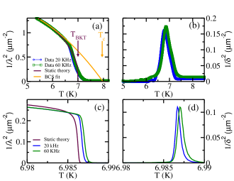
Figure 3: (Color online) Comparison between the experimental measurements (symbols) of $\lambda^{-2}$ (a) and $\delta^{-2}$ (b) and the predictions (solid lines) (c,d) of the conventional dynamical BKT theory for $D=10^{-5}$m${}^{2}/$s.The BCS fit in (a) works well far from the transition and allows one to estimate the BCS transition temperature $T_{c}$, while $T_{BKT}$ (obtained by using $\mu/J=1.2$) marks here the prediction of the homogeneous, static case. By using a conventional estimate of the vortex diffusion constant one obtains the rounding of $\lambda^{-2}$ shown in panel (c): as one can see it occurs on a temperature scale two orders of magnitude smaller than the one observed experimentally. At the same time, the peak in $\delta^{-2}$ shown in panel (d) is essentially a delta-like peak when compared to the measurements reported in panel (b).

The failure of the standard BKT dynamical theory for a homogeneous system shown in Fig. 3 is a clear indication that some crucial ingredient is missing. It is worth noting that the same theoretical approach was shown to be instead in very good quantitative agreement with experimental data in He films investigated in the past.ambegaokar_prb80 ; bishop_prb80 One crucial difference between superfluid films and superconducting ones is that in the latter case vortex-antivortex interactions are screened out by charged supercurrenst, so that BKT physics becomes visible only for thin enough films.review_minnaghen ; review13 However, as the film thickness is reduced also the disorder level increases, putting thin BKT films on the verge of the SIT, where additional physical effects emerge. The most important one is the natural tendency of the system to form inhomogeneous SC structures, that modify crucially the above results derived for a purely homogeneous superconductor. In particular, as it has been discussed in a series of recent publications,mondal_prl11 ; yong_prb13 the inhomogeneity of the system is the main reason for the smearing out of the universal superfluid jump with respect to the BKT prediction (see Fig. 3a). However, as we shall see in the next Section, the analysis of the dissipative part shows that the inhomogeneity can have also a strong effect on the ability of vortices to diffuse under an ac field, explaining the anomalously large resistive signal observed in the experiments.

IV Dynamical BKT theory in the presence of inhomogeneity

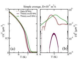
Figure 4: (Color online) Comparison between the experimental data and the complex conductivity computed as the average over an inhomogeneous Gaussian distribution ($\sigma_{G}/\bar{J}=0.015$) of local superfluid-stiffness values for a conventional value of $D=10^{-5}$ m²/s. While this procedure works very well for the inductive response (a), leading to the smearing of the BKT jump, it does not capture at all the intensity of the dissipative response (b) observed experimentally in the kHz frequency range.

A first root to account for inhomogeneity is a direct extension of the procedure proposed in Refs. [mondal_prl11, ; yong_prb13, ] in the static case, i.e. an average of the conductivity over a distribution $P(J_{i})$ of local superfluid-stiffness values $J_{i}$, that mimic in a simple macroscopic picture the spatial inhomogeneity observed by STM.sacepe_11 ; pratap_13 ; noat_prb13 Here we extend this approach to the complex conductivity $\sigma(\omega)$, computed for each patch according to Eq. (6), while the global one is given by an average $\sigma=\int dJ_{i}P(J_{i})\sigma_{i}(\omega)$ over a Gaussian distribution $P(J_{i})=(1/\sqrt{2\pi}\sigma_{G})\exp[-(J_{i}-\bar{J})^{2}/2\sigma_{G}^{2}]$ of local superfluid-density values. Here each $J_{i}(T)$ follows from the numerical solution of the BKT RG equations, using as initial value a BCS expression, such that $\bar{J}(T)$ has as starting point the BCS fit of low-temperature data shown in Fig. 2 (see details in Ref. [yong_prb13, ]). The complex conductance of each patch follows then from Eq. (6) above. The resulting $\sigma(\omega)$ for a conventional value of the diffusion constant, i.e. $D\sim 10^{-5}$ m²/s, is shown inFig. 4a. As we discussed above, finite-frequency effects have a negligible impact on the stiffness $\lambda_{i}^{-2}$ of each patch (see Fig. 3c), so at $\omega=$20 kHz the average superfluid response is practically the same computed in Refs. [mondal_prl11, ; yong_prb13, ] for the static case. As one can see, since within patches with smaller/larger local $J_{i}$ values the transition occurs at lower/higher temperatures, the average stiffness displays a smeared transition, in good agreement with the experimental data. This support the notion, already pointed out in previous work,mondal_prl11 ; yong_prb13 that the main source of the superfluid-density jump smearing is the inhomogeneous distribution of local transition temperatures, while finite-frequency effects are not so relevant. When applied to the dissipative finite-frequency vortex response the averaging procedure has the analogous effect: the delta-like peak found at $20$ kHz for $\delta_{i}^{-2}$ in each patch is now convoluted with a Gaussian distribution of local transition temperatures, leading to a widening of the peak. However, this has also the unavoidable effect of reducing the peak intensity, that is now at $\omega=20$ kHz two orders of magnitude smaller than what observed experimentally, see Fig. 4b. In addition, while the inductive response is weakly dependent on the frequency, the dissipative one increases strongly when we move in the microwave regime, even after the average procedure. The peak in $\delta^{-2}$ shown in Fig. (4)b at $\omega=2$ GHz for a conventional value of the vortex diffusion constant is instead of the correct order of magnitude, even if the shape of the peak is still different.

The strong disagreement between the experiments and the theory in the kHz frequency range suggests that the length scale $r_{\omega}$ for vortex diffusion is the same expected in the microwave regime, so that $D$ must be taken in our simulation a function of frequency strongly decreasing at low $\omega$. Notice also that the simple average procedure leads to an overestimate of the transition width in $\sigma_{1}$ at large frequency, see Fig. (4)b. To improve the treatment of the finite-frequency effect we then resort to a self-consistent effective-medium approximationema (SEMA) for the optical conductivity of the inhomogeneous system. Thus, once generated a distribution of local $\sigma_{i}(\omega)$ conductance with probability $P_{i}\equiv P(J_{i})$ the complex SEMA conductance $\sigma(\omega)$ is computed as the solution of the following equation:

$$\sum_{i}P_{i}\frac{\sigma_{i}(\omega)-\sigma(\omega)}{\sigma_{i}(\omega)+\eta\sigma(\omega)}.$$ (22)

where $\eta=D-1$ coincides with 1 in two spatial dimensions. Notice that Eq. (22) can also be rewritten as:

$$\sigma=\left((1+\eta)\sum_{i}\frac{P_{i}}{\sigma_{i}+\eta\sigma}\right)^{-1},$$ (23)

so that one sees that in the limiting case $\eta=0$ $\sigma$ is computed by assuming that the complex impedances are in series, as it is the only possible case in $D=1$ physical dimensions. In this situation the contribution of each single resistor to the overall dissipative response in enhanced: indeed, for $\eta=0$ at each temperature $\sigma$ is dominated by the resistor $\sigma_{i}$ having a peak at that temperature, weighted as $1/P_{i}$ instead of $P_{i}$ that one had in the simple average procedure. Thus the use of the effective-medium approximation amplifies in general the dissipative response of our network of BKT complex conductances, getting a better agreement with the experiments. For what concerns instead $\sigma_{2}$ the SEMA conductance behaves essentially as the averaged one, with a general smoothening of the superfluid-density jump due to the superposition of several $J_{s}^{i}(T)$ curves vanishing at different temperatures.

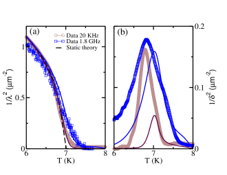
Figure 5: (Color online) Inductive (a) and resistive (b) response of the SEMA complex conductivity from Eq. (22). The same color is used for the experimental data (symbols) and the theoretical curves (solid lines). The dashed black line in panel (a) corresponds to the superfluid response in the static limit. The value of the diffusion coefficient $D$ at the various frequencies is reported in the text. The remaining parameters for the BCS fit are the same of Fig. 2 and Fig. 3a, while the BKT parameters are slightly different due to the different averaging procedure, i.e. $\sigma_{G}/\bar{J}=0.02$ and $\mu/\bar{J}=1.18$.

In Fig. 5 we show results for the complex SEMA conductance obtained with $D\simeq 10^{-11}$ m²/s in the kHz regime, corresponding to a $r_{\omega}\simeq 8\xi_{0}$ at $\omega=20$ kHz. In the kHz regime the dissipative response of each local impedance is highly enhanced with respect to the results of Fig. 4, and the $\sigma_{1}$ peak is in better agreement with the experiments. In the microwave regime instead $D$ increases, and a good compromise between the fit of the inductive and dissipative response is found for a conventional value $D=1.5\times 10^{-5}$ m²/s, corresponding to $r_{\omega}\simeq\xi_{0}$ at $\omega=1.8$ GHz. Observe however that still the experimental data of Fig. 1 show a dependence on the probing frequency more pronounced than what found theoretically. This is a consequence of the weak (logarithmic) dependence of the vortex dielectric function on the scale $r_{\omega}$, as evidence for example by the estimate (20) of the peak temperature of each resistor.

V Discussion and Conclusions

As one can see in Fig. 5, even accounting for the slow vortex diffusivity and the system inhomogenity the agreement with the experimental results for $\sigma_{1}$ in the kHz regime is not as good as the one for $\sigma_{2}$. On the other hand, the present phenomenological analysis, where the spatial inhomogeneity of the system is included in an effective-medium approach with a frequency-induced length-scale cut-off, elucidates already the emergence of a peculiar interplay between the inductive and resistive response near the BKT transition. In particular, by having in mind also theoretical results on disordered films.seibold_prl12 our results can be interpreted by assuming that the superfluid inductive response can take advantage of the existence of preferential (quasi one-dimensional) percolative paths connecting the good SC regions, while thermally-excited vortices responsible for the dissipation will mainly proliferate far away from the SC region. This notion is further supported by the emergence of an intrinsic length scale for vortex diffusion $r_{\omega}\sim\xi_{V}\sim 10-50$ nm that correlates very well with the typical size of the SC granularity observed experimentally by STM experiments,sacepe_11 ; pratap_13 ; noat_prb13 and predicted theoretically in microscopic models for disorder.ioffe ; nandini_natphys11 ; seibold_prl12 ; lemarie_prb13 Such a mechanism could thus explain the coexistence of both a large superfluid and dissipative response in a wide temperature range around the transition.

The quantitative comparison presented here between the theoretical prediction of a conventional BKT approach for homogeneous films and the experiments shows also that some care must be taken while analysing the data with a standard scaling approach,ffh as suggested for example for microwave measurements in thin InOx films in Ref. [armitage_prb11, ]. Indeed, we have shown that the shape of the complex conductivity is strongly affected by the inhomogeneous distribution of local SC properties. For example, even in the microwave regime the broadening of the superfluid-density jump cannot be understood as a trivial finite-frequency effect, as it is instead assumed in the usual scaling hypothesis.ffh ; armitage_prb11 Thus, the extractionarmitage_prb11 of a scaling frequency $\omega_{0}(T)$ that correlates with the usual BKT behaviour (18) of the vortex correlation length does not mean in general that a standard BKT scaling, i.e. the one predicted in the homogeneous BKT theory, is at play. Indeed, the real agreement with BKT scaling should be proven by comparing in a qualitative and quantitative way the complex conductance itself. In our case, we checked explicitly that even though the microwave data can be rescaled to give a BKT-like scaling frequency $\omega_{0}(T)$, the scaling function itself deviates strongly from the BKT one, since its shape is controlled by the inhomogeneity. In addition, while we focused here on thin film where the transition has BKT character, the peculiar role of inhomogeneity is a general feature of disordered films near the SIT. Indeed, the strong slowing down of the fluctuation conductivity observed recently in thick NbN films,mondal_scire13 where BKT physics is absent, show that the enhanced finite-frequency effects reported near the SIT can be analogously interpreted as a signature of an intrinsic length-scale dependence associated to inhomogeneous SC domains.

Finally, the present analysis clarifies also that the absence of a sharp superfluid-density jump in thin films of conventional superconductors cannot be attributedyazdani_prl13 to the the mixing between inductive and reactive response that already occurs at the kHz frequency. Indeed, in the standard homogeneous case the effect of the frequency on the universal jump would be the one shown in Fig. 3c, i.e. the $\lambda^{-2}$ should still drop to zero so rapidly to appear as a discontinuous jump in the experiments. The rounding effect of the stiffness are instead entirely due to the inhomogeneity, that also mixes in a non-trivial way inductive and reactive response, making it meaningless the extraction from the data of the inverse inductance in order to analyse the superfluid-density jump, as done e.g. in Ref. [yazdani_prl13, ] (see also Appendix A).

In summary, we analysed the occurrence of the dynamical BKT transition in thin films of NbN. We measured the same samples both in the kHz regime, where dynamical effects should be negligible according to the standard view, and in the microwave regime, where one would expect instead a sizeable finite-frequency induced dissipative response. Our experimental results show a consistent broadening of the universal BKT superfluid-density jump, that can be attributed to inhomogeneity, and an anomalously large resistive response in the low-frequency range, that cannot be understood by means of a standard value of the vortex diffusion constant. By making a quantitative comparison between the experiments and the theoretical predictions for the BKT physics in a inhomogeneous SC environment we show that the dissipative response in the kHz regime can only be understood by assuming a low vortex diffusivity. This effect limits the vortex motion over an intrinsic length scale of the order of the typical size of homogeneous SC domains observed by STM near the SIT. While the present approach accounts for the emergence of SC inhomogeneity in a phenomenological way, a more microscopic approach is certainly required to understand how the BKT vortex physics can accommodate to the disorder-induced SC granularity by preserving its general character.

Appendix A Dielectric function of vortices within the RG approach

The expression for the vortex dielectric constant $\varepsilon(\omega)$ that appears in Eq. (6) has been derivedambegaokar_prb80 ; HN by exploiting the analogy between the Coulomb gas and the vortices. It contains two contribution, one $\varepsilon_{b}$ due to bound vortex-antivortex pairs that exist already below $T_{BKT}$, and one $\varepsilon_{f}$ due to free single-vortex excitations that are thermally excited above $T_{BKT}$. To compute $\varepsilon_{b}$ one exploits the idea that under the applied oscillating field vortices experience a Langevin dynamics controlled by the diffusion constant $D$. In practice, if we think that in the BKT theory what controls $J_{s}(r)$ is the screening due to neutral vortex-antivortex pairs at a scale $r$, dynamics introduces one additional scale $r_{\omega}$ such that pairs with separation $r\gg r_{\omega}$ will not contribute to the polarization since they will change the relative orientation over a cycle of the oscillating field. This explains while $\varepsilon_{b}$ is cut-off at $r_{\omega}$. On the other hand free vortices have uncorrelated motions with respect to each other and, when present, they will contribute directly to dissipation. The general expressions for the bound $\varepsilon_{b}$ and free $\varepsilon_{f}$ vortex contributions are then:ambegaokar_prb80

$$\varepsilon_{b}(\omega) = 1+\int_{\xi_{0}}^{\xi}dr\frac{d\tilde{\varepsilon}(r)}{dr}\frac{14Dr^{-2}}{-i\omega+14Dr^{-2}}$$ (24)

$$\varepsilon_{f}(\omega) = i\frac{4\pi^{2}J}{k_{B}T}\frac{Dn_{f}}{\omega}=i\frac{2\pi^{2}J}{7k_{B}T}\left(\frac{r_{\omega}}{\xi}\right)^{2}$$ (25)

where $n_{f}$ is the free-vortex density, expressed in terms of the correlation length $\xi$ as $n_{f}={1}/{\xi^{2}}$, $J$ is the superfluid stiffness defined in Eq. (7) above and $\tilde{\varepsilon}$ is defined in terms of the RG variable $K$ (8) as

$$\tilde{\varepsilon}(r)=\left.\frac{K(0)}{K(\ell)}\right|_{\ell=\ln(r/\xi_{0})}.$$ (26)

Let us first analyze the case of an infinite system at $\omega=0$. When the system is infinite the correlation length $\xi=\infty$ below $T_{BKT}$. In this case the upper limit of integration in Eq. (24) is set at $\infty$ and the free-vortex contribution is different from zero only above $T_{BKT}$. Morevoer, by using $\omega=0$ $\varepsilon_{b}$ (and then also the total $\varepsilon$) is purely real and it can be easily computed using the definition (26): indeed we have that

$$\varepsilon_{b}(\omega=0) = 1+\int_{a_{0}}^{\infty}dr\frac{d\tilde{\varepsilon}(r)}{dr}=1+\tilde{\varepsilon}(\infty)-\tilde{\varepsilon}(\xi_{0})$$ (27)

$$= \tilde{\varepsilon}(\infty)=\frac{K(0)}{K(\infty)}=\frac{J(0)}{J_{s}}$$

in agreement with Eq. (12) above, where we already used the definition (13) $J(\ell=\infty)=J_{s}$. Since $J(0)\propto n_{s}^{0}$ while $J_{s}\propto n_{s}$, where $n_{s}$ is the real superfluid density including also the vortex contribution we obtain in Eq. (6) that at $\omega=0$ the response is purely inductive:

$$\sigma(\omega=0)=-\frac{n_{s}de^{2}}{i\omega m}.$$ (28)

At finite frequency the dielectric function develops an imaginary part, responsible for the dissipative response detected via $\sigma_{1}$. Bound vortices give the main contribution to the real part of the dielectric function, while free vortices occurring on the length scale $r_{\omega}$ contribute to the imaginary part of the dielectric function. All the theoretical results shown in the mansuscript have been obtained by means of the full numerical solution (24)-(25), where $K(\ell)$ is the solution of the RG equations (8)-(9). On the other hand, one can also provide a rough estimate of the expected behavior of complex conductivity based on the above formulas. For what concern $\varepsilon_{1}$ the contribution of bound vortices at finite frequency can be estimated by replacing in Eq. (27) above the upper cut-off of integration with $r_{\omega}$, that is that maximum distance explored by vortices under the applied field.ambegaokar_prb80 One then has:

$$\varepsilon_{1}(\omega)={\varepsilon_{b}}_{1}(\omega)\approx\frac{K(0)}{K(\ell_{\omega})}$$ (29)

so that instead of the discontinuous jump of $\varepsilon_{1}$ expected at $\omega=0$ one observes now a rapid but continuous downturn, as discussed in Sec. III. At the same time for $\varepsilon_{2}$ one has the largest contribution from free vortices, i.e. the contribution (25) above that has been discussed below Eq. (15) in Sec. III. Notice that in the homogeneous case Eq. (6) and (29) above show that if one plot directly the inverse inductance, as it has been sometimes suggested,yazdani_prl13 i.e

$$L^{-1}=\frac{n_{s}^{0}e^{2}d}{m\varepsilon_{1}(\omega)}\approx\frac{n_{s}(r_{\omega})e^{2}d}{m},$$ (30)

then one can directly access the superfluid-density jump occurring at finite frequency. However, while this would be a viable procedure to isolate the real and imaginary part of the dielectric function for a homogeneous system, it fails completely in the presence of inhomogeneity, that has a much more drastic effect on the jump than the finite-frequency behaviour. Thus in the case of thin disordered films the lack of a sharp BKT jump cannot be circumvented by extracting from the measured conductivity the inverse inductance, since this procedure mixes in an artificial and uncontrolled way the non-trivial effects of the inhomogeneity on the finite-frequency response.

References

- (1) P. Minnhagen, Rev. Mod. Phys. 59, 10001 (1987).
- (2) For a recent review see "40 years of Beresinskii-Kosterlitz-Thouless theory" edited by Jorge V. Josè, World Scientific (2013).
- (3) V.L.Beresinkii, Sov. Phys. JETP 34, 610 (1972); J.M.Kosterlitz and D.J.Thouless, J. Phys. C 6, 1181 (1973).
- (4) J.M.Kosterlitz, J. Phys. C 7, 1046 (1974).
- (5) D.R.Nelson and J.M.Kosterlitz, Phys. Rev. Lett. 39, 1201 (1977).
- (6) D. McQueeney, G. Agnolet, and J. D. Reppy, Phys. Rev. Lett. 52, 1325 (1984).
- (7) S. J. Turneaure, T. R. Lemberger and J. M. Graybeal, Phys. Rev. B 63, 174505 (2001).
- (8) S. Misra, L. Urban, M. Kim, G. Sambandamurthy, and A. Yazdani, Phys. Rev. Lett. 110, 037002 (2013)
- (9) A.T.Fiory, A.F.Hebard and W.I.Glaberson, Phys. Rev. B28, 5075 (1983)
- (10) R.W. Crane, N. P. Armitage, A. Johansson, G. Sambandamurthy, D. Shahar, and G. Gruner, Phys. Rev. B75, 094506 (2007)
- (11) W. Liu, M. Kim, G. Sambandamurthy and N.P. Armitage, Phys. Rev. B 84, 024511 (2011).
- (12) A. Kamlapure, M. Mondal, M. Chand, A. Mishra, J. Jesudasan, V. Bagwe, L. Benfatto, V. Tripathi and P. Raychaudhuri, Appl. Phys. Lett. 96, 072509 (2010).
- (13) M. Mondal, S. Kumar, M. Chand, A. Kamlapure, G. Saraswat, G. Seibold, L. Benfatto, P. Raychaudhuri, Phys. Rev. Lett. 107, 217003 (2011).
- (14) Jie Yong, T. Lemberger, L. Benfatto, K. Ilin, M. Siegel, Phys. Rev. B 87, 184505 (2013).
- (15) See e.g. Jie Yong, M. J. Hinton, A. McCray, M. Randeria, M. Naamneh, A. Kanigel, and T. R. Lemberger, Phys. Rev. B85, 180507 (2012) and references therein.
- (16) Julie A. Bert, Katja C. Nowack, Beena Kalisky, Hilary Noad, John R. Kirtley, Chris Bell, Hiroki K. Sato, Masayuki Hosoda, Yasayuki Hikita, Harold Y. Hwang, and Kathryn A. Moler, Phys. Rev. B86, 060503(R) (2012).
- (17) B.Sacepe, C. Chapelier, T. I. Baturina, V. M. Vinokur, M. R. Baklanov, M. Sanquer, Nature Communications 1, 140 (2010). B. Sacépé et al., Nature Phys. 7, 239 (2011).
- (18) M. Mondal, A. Kamlapure, M. Chand, G. Saraswat, S. Kumar, J. Jesudasan, L. Benfatto, V. Tripathi, and P. Raychaudhuri, Phys. Rev. Lett. 106 047001 (2011).
- (19) A. Kamlapure, T. Das, S. Chandra Ganguli, J. B. Parmar, S. Bhattacharyya, and P. Raychaudhuri, Sci. Rep. 3, 2979 (2013).
- (20) Y. Noat, V. Cherkez,,C. Brun,T. Cren, C. Carbillet, F. Debontridder, K. Ilin, M. Siegel, A. Semenov, H.-W. H ubers, D. Roditchev, Phys. Rev. B88, 014503 (2013).
- (21) L. B. Ioffe and M. Mezard, Phys. Rev. Lett. 105, 037001 (2010); M.V. Feigelman, L. B. Ioffe, and M.Mezard, Phys. Rev. B 82, 184534 (2010).
- (22) K. Bouadim, Y. L. Loh, M. Randeria, and N. Trivedi, Nat. Phys. 7, 884 (2011).
- (23) G. Seibold, L. Benfatto, C. Castellani, J. Lorenzana, Phys. Rev. Lett. 108, 207004 (2012).
- (24) G. Lemari«e, A. Kamlapure, D. Bucheli, L. Benfatto, J. Lorenzana, G. Seibold, S. C. Ganguli, P. Raychaudhuri, and C. Castellani, Phys. Rev. B 87, 184509 (2013).
- (25) L. Benfatto, C. Castellani and T. Giamarchi, Phys. Rev. B 77, 100506(R) (2008).
- (26) L. Benfatto, C. Castellani and T. Giamarchi, book chapter in "40 years of Beresinskii-Kosterlitz-Thouless thoery" edited by Jorge V. José, World Scientific (2013).
- (27) V. Ambegaokar et al., Phys. Rev. B21, 1806 (1979).
- (28) B. I. Halperin and D. R. Nelson, J. Low. Temp. Phys. 36, 599 (1979).
- (29) S.J. Turneaure, E.R. Ulm, T.R. Lemberger, J. Appl Phys. 79,4221(1996).
- (30) S.J. Turneaure, A.A. Pesetski, T.R. Lemberger, J. Appl. Phys. 83,4334(1998).
- (31) M. Mondal, Phd thesis, arXiv.1303.7396v2.
- (32) M. Mondal et al. Sci. Rep. 3, 1357 (2013).
- (33) H. Kitano, T. Ohashi, A. Maeda,e. Rev. Sci. Instrum. 79, 074701 (2008).
- (34) M. Scheffler,M. Dressel, Rev. Sci. Instrum. 76, 074702 (2005).
- (35) J.C. Booth, D.H. Wu, S.M. Anlage, . Rev. Sci. Instrum. 65, 2082 (1994).
- (36) Fisher, Fisher and Huse, Phys. Rev. B43, 130 (1991)
- (37) M. Mondal et al. J Sup. Nov. Magn. 24, 341 (2011).
- (38) D. J. Bishop and J. D. Reppy, Phys. Rev. B22, 5171 (1980).
- (39) L. Benfatto, C. Castellani and T. Giamarchi, Phys. Rev. B 80, 214506 (2009).
- (40) S. Kirkpatrick, Rev. Mod. Phys. 45, 574 (1973).