High-order well-balanced finite-volume schemes for barotropic flows.
Development and numerical comparisons.

Abstract.

In this paper we compare a classical finite-difference and a high order finite-volume scheme for barotropic ocean flows. We compare the schemes with respect to their accuracy, stability, and study various outflow and inflow boundary conditions. We apply the schemes to the problem of eddy formation in shelf slope jets along the Ormen Lange section of the Norwegian shelf. Our results strongly confirm the development of mesoscale eddies caused by instability of the flows.

1. Introduction

In medium-scale geophysical fluid flow, with length scales of hundreds of kilometres, the geometry of the earth, its rotation and curvature are of great importance. The modelling of flow phenomena at these scales involves complex nonlinear equations with extra terms accounting for the geometry and the rotating frame of reference.

Many geophysical flow problems are shallow in the sense that the waves length of horizontal motion greatly exceeds the scale of changes in the vertical direction. In many cases, this justifies a simplification of the governing equations for the vertical motion. The shallow-water equations is one such system where the dependent variables are depth-averaged and only first-order differential terms are retained. In this paper we consider numerical solutions of the shallow-water system, written as a system of first-order hyperbolic conservation laws with source terms modelling the effects of variable bottom and a rotating frame of reference,

(1) $$\begin{bmatrix}\eta\\[4.26773pt] U\\[4.26773pt] V\end{bmatrix}_{t}+\begin{bmatrix}U\\[4.26773pt] \frac{U^{2}}{H}+\frac{1}{2}gH^{2}\\[4.26773pt] \frac{UV}{H}\end{bmatrix}_{x}+\begin{bmatrix}V\\[4.26773pt] \frac{UV}{H}\\[4.26773pt] \frac{V^{2}}{H}+\frac{1}{2}gH^{2}\end{bmatrix}_{y}=\begin{bmatrix}0\\[4.26773pt] -gHz_{x}+fV\\[4.26773pt] -gHz_{y}-fU\end{bmatrix}.$$

Here subscripts denote differentiation, $\eta$ is the surface elevation, $z$ is the bottom topography and $H=\eta-z$ is the total water depth. The components of the volume-flux per unit length in the $x$- and $y$-direction are $U$ and $V$, respectively. The source terms in (1) model two different physical effects: the rotation and the variable bottom topography. The rotating frame of reference introduces a Coriolis force $[0,fV,-fU]^{T}$ acting transversely and proportionally to the volume-flux. The other source term $[0,-gHz_{x},-gHz_{y}]^{T}$ accounts for the variations in the bottom topography $z$. In applications, this barotropic model is used to study weather systems, mean currents and transport and wave phenomena in coastal zones, rivers and lakes, in cases where the density stratification has negligible influence on the flow.

Classically, i.e. at least since the 1940s, such initial value problems have been solved by finite-difference methods [17, 20]. To this day, such methods are the working horse of many models. They are easy to implement, fast, and for smooth flows they give accurate results. On the other hand, for non-smooth solutions they suffer from dispersive oscillations which need to be damped by adding artificial viscosity.

These stability problems led (roughly from 1950s into the 1990s) to the development of more robust finite-difference, finite-volume, ENO and WENO schemes [13, 10, 14, 11, 15, 24]. For geophysical flows it was important to develop schemes which maintain fundamental equilibrium solutions on the discrete level, the so-called well-balanced schemes (see e.g. [1, 18, 27] and the references therein). Recently, Bouchut et al.[2] have described a technique to obtain a well-balanced discretisation of the Coriolis terms in the one-dimensional case. The well-balanced discretisation preserves geostrophically balanced states exactly at the discrete level. This technique may be generalised to two-dimensional jets which are aligned with a Cartesian grid. With these extensions, well-balanced finite-volume schemes are a very stable and – if equipped with high-order reconstructions – highly accurate alternative for the computation of depth-averaged geophysical flows, which may contain shock-, or bore-waves. An advantage of these schemes is that the solution is damped only in region where damping is needed.

The present paper reports on the joint work of a researcher, who has over many years developed and used a finite-difference ocean models [9], an engineer and two numerical analysts who have developed a high order well-balanced finite-volume scheme [18]. Our goal is to study and, if possible, quantify the advantages of either code. We hope that other researchers will draw some useful conclusions from our results, when they decide which type of code they should use.

As test-case we study a class of jets along the Norwegian shelf. Such shelf slope jets have been studied extensively (see [9, 26] and the references therein). A series of numerical examples indicates that these currents can become unstable, in the sense that an initially almost laminar flow generates strong eddies and oscillations. Linear stability analysis [9, 26] confirms the existence of unstable modes. This provides us with a challenging test problem within a relatively simple topography. Other test problems are used to study numerical convergence and accuracy.

It will come as no surprise that the setup of analytical and numerical in- and outflow boundary conditions was one of the main difficulties in this study.

The outline of the paper is as follows: In Section 2.1 we give an overview of the finite-difference method used in [9]. We rearrange the temporal update to assure second-order accuracy. In Sections 2.2 we review the high-order well-balanced finite-volume scheme derived recently in [18]. In particular, the source term treatment is described in Section 2.3. The entire Section 3 is devoted to boundary conditions, particularly inflow and absorbing outflow boundary conditions for the finite-volume scheme. These have a strong impact upon the accuracy and the flow features computed by our schemes. In Section 4, we evaluate the accuracy, order of convergence and resolution for various test problems. Then we focus on the formation of eddies in shelf slope jets. Here we study and thereby rule out several possible numerical sources of the instability. We conclude the paper in Section 5 by discussing in detail the advantages of the finite-difference and finite-volume solvers, the boundary conditions and the eddy formation in the along shelf current.
Acknowledgement: We would like to thank Roland Schäfer for lively and stimulating discussions. Also we would like to thank Frank Knoben and Markus Jürgens for there unresting support for the parallelisation of the scheme.

2. Discretisation

In this section we give an overview of the two numerical schemes. The philosophies underlying these schemes are quite different. In the finite-difference scheme, the solution is approximated by point values on a grid. To advance the solution, the derivative of the flux terms are computed using central differencing and averaging operators. A special staggering of variables, called a B-grid, is used, where the volume-flux is approximated on the mesh $(ih,jh,n\Delta t)$, and the surface elevation is approximated on a mesh shifted by $h/2$ in each spatial direction and $\Delta t/2$ in time. The original scheme of [9] is second-order accurate in space, but only first-order accurate in time. A simple extension yields a fully second-order finite-difference scheme. In actual computations, this scheme performs very well for smooth solutions. However, we do observe spurious oscillations when shocks appear in the solution. In Section 2.1 we give a complete description of this scheme.

In the finite-volume scheme, the solution is approximated in terms of cell-averages. These cell averages are advanced in time by computing fluxes across cell interfaces. To evaluate the fluxes, accurate point-values of each variable must be reconstructed from cell averages. We use a fifth-order WENO procedure [23, 24] for the reconstruction combined and Roe’s approximate Riemann solver [21] for the interface flux. A standard fourth-order Runge-Kutta scheme is used as temporal discretisation. In addition, the scheme is equipped with a high-order well-balanced discretisation of the geometrical source term [18]. This scheme has proven to be highly accurate both for smooth and non-smooth solutions. In Section 2.2 we give an overview of this scheme, and refer to [18] for a full description.

2.1. The Finite-Difference Scheme and a fully second-order accurate extension

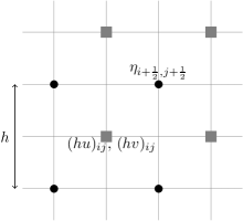
Figure 1. The layout of a B-grid. The surface elevation $\eta$ is approximated in the black circles, and the volume-fluxes $U$ and $V$ in the grey squares.

The original B-grid scheme of [9] is based on a staggering of unknowns, where the volume-fluxes $U$ and $V$ are approximated in the grid points $(ih,jh,n\Delta t)$ and the surface elevation $\eta$ is approximated in shifted grid points $((i+\frac{1}{2})h,(j+\frac{1}{2})h,(n+\frac{1}{2})\Delta t)$ as shown in Figure 1. To ease the presentation we introduce the following standard differencing and averaging operators:

$$\begin{array}[]{l@{\quad\quad\quad}r}\delta_{x}()_{\cdot,\cdot}=\frac{1}{h}\left[()_{\cdot+\frac{1}{2},\cdot}-()_{\cdot-\frac{1}{2},\cdot}\right],&\mu_{x}()_{\cdot,\cdot}=\frac{1}{2}\left[()_{\cdot+\frac{1}{2},\cdot}+()_{\cdot-\frac{1}{2},\cdot}\right],\\[8.5359pt] \delta_{y}()_{\cdot,\cdot}=\frac{1}{h}\left[()_{\cdot,\cdot+\frac{1}{2}}-()_{\cdot,\cdot-\frac{1}{2}}\right],&\mu_{y}()_{\cdot,\cdot}=\frac{1}{2}\left[()_{\cdot,\cdot+\frac{1}{2}}+()_{\cdot,\cdot-\frac{1}{2}}\right].\end{array}$$

Note that it is implied that the result of these operations is shifted by $\frac{h}{2}$ relative to the argument. For simplicity in notation, we omit $i$ and $j$ indices in the following scheme. The meaning should be clear from the aforementioned shift and the position of the point-wise approximations. For instance, the approximation of $\partial_{x}(U^{2}/H)$ in the point $(ih,jh)$ is given by

$$\left(\delta_{x}\frac{\big{(}\mu_{x}U\big{)}^{2}}{\mu_{y}H}\right)_{ij} =\frac{1}{2h}\left(\frac{\big{(}U_{i+1,j}+U_{ij}\big{)}^{2}}{H_{i+\frac{1}{2},j-\frac{1}{2}}+H_{i+\frac{1}{2},j+\frac{1}{2}}}-\frac{\big{(}U_{ij}+U_{i-1,j}\big{)}^{2}}{H_{i-\frac{1}{2},j-\frac{1}{2}}+H_{i-\frac{1}{2},j+\frac{1}{2}}}\right)$$

With this notation, we can write the finite-difference scheme for (1) as

(2) $$\eta^{n+\frac{1}{2}} =\eta^{n-\frac{1}{2}}-\Delta t[\delta_{x}\mu_{y}U^{n}+\delta_{y}\mu_{x}V^{n}]$$

(3) $$U^{n+1} =U^{n}-\Delta t\left[\delta_{x}\frac{\big{(}\mu_{x}U^{n}\big{)}^{2}}{\mu_{y}H^{n+\frac{1}{2}}}+\delta_{y}\frac{\big{(}\mu_{y}U^{n}\big{)}\;\big{(}\mu_{y}V^{n}\big{)}}{\mu_{x}H^{n+\frac{1}{2}}}+\big{(}g\mu_{x}\mu_{y}H^{n+\frac{1}{2}}\big{)}\delta_{x}\mu_{y}\eta^{n+\frac{1}{2}}-fV^{n}\right],$$

(4) $$V^{n+1} =V^{n}-\Delta t\left[\delta_{x}\frac{\big{(}\mu_{x}U^{n}\big{)}\;\big{(}\mu_{x}V^{n}\big{)}}{\mu_{y}H^{n+\frac{1}{2}}}+\delta_{y}\frac{\big{(}\mu_{y}V^{n}\big{)}^{2}}{\mu_{x}H^{n+\frac{1}{2}}}+\big{(}g\mu_{x}\mu_{y}H^{n+\frac{1}{2}}\big{)}\delta_{y}\mu_{x}\eta^{n+\frac{1}{2}}+fU^{n}\right],$$

where $\Delta t$ is the time step and $H^{n+\frac{1}{2}}=\eta^{n+\frac{1}{2}}-z$. The use of a B-grid yields a quite compact second-order discretisation of the flux and source terms. We would like to point out that, due to the central differencing, the scheme (2)–(4) is second order accurate in space, but not in time. This can be seen most easily from left part of Figure 2, which shows that the stencil of the volume-flux update is not symmetric with respect to time.

In order to correct the asymmetry, we introduce the following shorthands:

$$\Phi_{x}(\eta) :=\big{(}g\mu_{x}\mu_{y}H\big{)}\delta_{x}\mu_{y}\eta,$$

$$\Phi_{y}(\eta) :=\big{(}g\mu_{x}\mu_{y}H\big{)}\delta_{y}\mu_{x}\eta,$$

$$\Omega(U,V,\eta) :=\delta_{x}\frac{\big{(}\mu_{x}U\big{)}^{2}}{\mu_{y}H}+\delta_{y}\frac{\big{(}\mu_{y}U\big{)}\;\big{(}\mu_{y}V\big{)}}{\mu_{x}H}-fV,$$

$$\Psi(U,V,\eta) :=\delta_{x}\frac{\big{(}\mu_{x}U\big{)}\;\big{(}\mu_{x}V\big{)}}{\mu_{y}H}+\delta_{y}\frac{\big{(}\mu_{y}V\big{)}^{2}}{\mu_{x}H}+fU.$$

where $H=H(\eta,z)$. With this notation (3) – (4) read

(5) $$U^{n+1} =U^{n}-\Delta t\left[\Omega(U^{n},V^{n},\eta^{n+\frac{1}{2}})+\Phi_{x}(\eta^{n+\frac{1}{2}})\right],$$

(6) $$V^{n+1} =V^{n}-\Delta t\left[\Psi(U^{n},V^{n},\eta^{n+\frac{1}{2}})+\Phi_{y}(\eta^{n+\frac{1}{2}})\right].$$

Let us now introduce the correction which assures second order accuracy in time. For this we denote the volume-flux update in (5) – (6) by $(U,V)^{n+1}_{*}$ and centre the terms $\Omega$ and $\Psi$, i.e the flux differences and the coriolis term, with respect to time. This gives

(7) $$U^{n+1} =U^{n+1}_{*}+\frac{\Delta t}{2}\left[\Omega(U^{n},V^{n},\eta^{n+\frac{1}{2}})-\Omega(U^{n+1}_{*},V^{n+1}_{*},\eta^{n+\frac{1}{2}})\right],$$

(8) $$V^{n+1} =V^{n+1}_{*}+\frac{\Delta t}{2}\left[\Psi(U^{n},V^{n},\eta^{n+\frac{1}{2}})-\Psi(U^{n+1}_{*},V^{n+1}_{*},\eta^{n+\frac{1}{2}})\right],$$

which is the symmetric stencil shown in right part of Figure 2.

Figure 2. Stencils of volume-flux update for finite-difference schemes. Left: first order scheme, not symmetric with respect to time. Right: time symmetry recovered.

In Tables 1 and 2 one can clearly observe the gain in accuracy.

An elementary calculation shows that both the first-order version and the second-order version of this scheme are well-balanced for the stationary state of water at rest $U=V=0$ and $\eta-z=Const$. For smooth solutions driven by inflow boundary conditions, both scheme yields quite sharp results with moderate numerical diffusion. For non-smooth solutions, both versions of the scheme experience instabilities in the form of oscillations.

2.2. The High-Order Finite-Volume Scheme

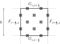
Figure 3. A finite-volume, with corresponding fluxes and integration points on cell interfaces and in the interior. The integration points in the interior are needed for the well-balanced integration rule for the source source term.

To simplify the presentation of the finite-volume scheme somewhat, we rewrite (1) as

(9) $$Q_{t}+F(Q)_{x}+G(Q)_{y}=B(Q,Q_{x},Q_{y})+C(Q),$$

where subscript denotes differentiation, $Q=[\eta,U,V]^{T}$ is the vector of unknown functions and $F$ and $G$ are vector-valued functions. The source terms $B=-gH[0,z_{x},z_{y}]^{T}$ and $C=f[0,V,-U]^{T}$ are the geometrical source accounting for variable bottom and the Coriolis force term, respectively.

The discretisation of the homogeneous part of (9) is straightforward. As opposed to the scheme in the previous section, the high order finite-volume scheme is based on computing cell averages over grid cells $I_{ij}=\left[\left(i-\frac{1}{2}\right)h,\left(i+\frac{1}{2}\right)h\right]\times\left[\left(j-\frac{1}{2}\right)h,\left(j+\frac{1}{2}\right)h\right]$ of a uniform Cartesian mesh. In each grid cell we approximate

$$\bar{Q}^{n}_{ij}=\int\!\!\!\int_{I_{ij}}Q(x,y,t^{n})dxdy.$$

To compute the evolution of the cell averages $\eta_{ij}$, $U_{ij}$ and $V_{ij}$, we must approximate the flux over the cell interfaces. This is accomplished by reconstructing the solution within each grid cell using (nonlinear) interpolation. To obtain a stable and accurate solution, the reconstruction procedure must ensure that no spurious oscillations are introduced, even when the solution is non-smooth. This may be done, for example, by the WENO technique (see [24] and the references therein). The reconstruction yields one-sided approximations of point values at cell interfaces as well as in the interior of the cell, see Figure 3. Thus, at each cell interface we obtain two one-sided approximations. To compute consistent interface fluxes we integrate Roe’s approximate flux function $\hat{F}(Q^{+},Q^{-},n)$ [21] over each cell interface. In computations, these integrals are approximated using Gaussian quadrature. For the $x$-direction, $F_{i+\frac{1}{2},j}$ is computed as,

$$F_{i+\frac{1}{2},j} =\int_{(j-\frac{1}{2})h}^{(j+\frac{1}{2})h}\hat{F}\Big{(}Q\big{(}(i+\frac{1}{2})h,y\big{)}^{-},Q\big{(}(i+\frac{1}{2})h,y\big{)}^{+},n_{x}\Big{)}dy,$$

$$\approx h\sum_{\alpha}\omega_{\alpha}\hat{F}\Big{(}Q\big{(}(i+\frac{1}{2})h,y_{\alpha}\big{)}^{-},Q\big{(}(i+\frac{1}{2})h,y_{\alpha}\big{)}^{+},n_{x}\Big{)},$$

where $y_{\alpha}$ and $\omega_{\alpha}$ are the quadrature points and weights. The fluxes in the $y$-direction $G_{i,j+\frac{1}{2}}$ are computed in the same manner. To complete the spatial discretisation we must compute the averaged source terms $B_{ij}$ and $C_{ij}$ over each grid cell. The final evolution of the cell averages is computed by solving the semi-discrete equation

(10) $$\frac{d}{dt}\bar{Q}_{ij}=-(F_{i+\frac{1}{2},j}-F_{i-\frac{1}{2}},j)/h-(G_{i,j+\frac{1}{2}}-G_{i,j-\frac{1}{2}})/h+B_{ij}+C_{ij},$$

using a standard fourth-order Runge-Kutta scheme. The details of the source term discretisation are given in Section 2.3, and the boundary conditions are discussed in Section 3.2.

2.3. Well-balanced Finite-Volume Treatment of the Source Terms

The shallow water system has stationary solutions where source terms and flux terms are in equilibrium. If we discretise the fluxes and source terms naively, this may lead to spurious oscillations near equilibria. To accurately resolve small perturbations of such equilibria, we must ensure that the discrete fluxes and sources exactly balance at equilibrium. Ideally, the truncation error of the scheme should vanish at equilibrium states. This is often called a well-balanced treatment of source terms.

Flat, stationary water of variable depth is an equilibrium where it is possible to construct such a discretisation. In [18], an arbitrary-order well-balanced discretisation of the geometrical source term was constructed. A well-balanced second-order discretisation of the geometrical source term is extended to arbitrary order of accuracy using an asymptotic expansion. In a single grid cell in one spatial dimension, the integral of the source term can be approximated by the fourth-order rule

(11) $$S =\frac{g}{6}\left[4(\eta_{l}+\eta_{c})(z_{l}-z_{c})+4(\eta_{c}+\eta_{r})(z_{c}-z_{r})-(\eta_{l}+\eta_{r})(z_{l}-z_{r})\right]$$

where $\eta_{l}$, $\eta_{c}$ and $\eta_{r}$ are reconstructed point-values in the left-, centre- and right endpoints of the cell. The reconstruction of the central point is an additional cost associated with this source term. This integration rule can be extended to two spatial dimensions using Gaussian quadrature. In the equation for $x$-volume-flux, (11) is applied in the $x$-direction and the Gaussian rule in the $y$-direction. For the $y$-volume-flux, the order is reversed. The integration points used for the source terms are shown in Figure 3.

The Coriolis term is approximated by $C_{ij}=f[0,V_{ij},-U_{ij}]^{T}$. As in [2], this is well-balanced for grid-aligned geostrophic jets.

3. Treatment of boundary conditions

For the experiments presented in this paper we need three types of boundary conditions, reflective, outflow and inflow. These are presented below. While reflective boundaries are rather straightforward, out- and inflow conditions have to be translated carefully from the B-grid finite-difference setting to the finite-volume setting. Moreover, for the finite-volume scheme we discovered a subtle perturbation introduced by a no-slip inflow boundary condition. In Sections 3.2.3 and 3.2.4, we introduce free-slip, Neumann-type boundary conditions which give smoother inflow.

3.1. Finite-Difference Boundary Conditions

Reflective boundary condition are treated with one-sided differences and normal volume-flux equal zero. At outflow boundaries the normal volume-flux $V$ is defined by $\eta\sqrt{gH}$ and the transverse volume-flux $U$ is set to zero. This boundary condition is called Flather condition in mechanics, and it coincides e.g. with the first order absorbing boundary condition given by Engquist and Majda [6]. The normal velocity $v$ on the inflow boundary is given by a time dependent velocity profile function $v_{\textnormal{jet}}(x,y,t)$ (see (36) and (41)) and the tangential velocity $u$ is set to zero (no-slip). To compute the volume-flux on the inflow boundary the height is extrapolated from the interior. These boundary conditions are straightforward to implement in the finite-difference scheme.

3.2. Finite-Volume Boundary Conditions

3.2.1. Reflective boundary conditions

To treat reflective boundary conditions we are using ghost-cells and solve the Riemann problem on the reflective boundary, where the ghost cell contains the same data as the interior cell, but with reflected volume-fluxes.

3.2.2. Absorbing Outflow Boundary Condition

Here we adopt a technique developed by Engquist and Majda [6] to derive a so-called first order absorbing boundary conditions for the outflow boundary. In particular, we follow Kröner’s adaptation [12] of the Engquist-Majda absorbing boundary condition, who has computed the relevant decomposition into normal and tangential waves for the linearised Euler equations.

For the shelf flows which we would like to compute, there are two relevant cases. Due to the very large speed of long gravity waves in the ocean $c_{0}=\sqrt{gH}\gg v$ we are always in a subcritical flow and either one or two characteristics are leaving the domain. Carrying over the results of [6, 12] to the linearised shallow water equations, we obtain the following analytical boundary conditions:

If two characteristics are leaving the domain, the first order absorbing boundary conditions specifies the normal volume-flux $V=\eta\sqrt{gH}$ at the open boundary.

In the case of one outgoing characteristic we obtain as before $V=\eta\sqrt{gH}$ for the normal volume-flux. In addition, we obtain a no-slip condition for the tangential volume-flux, namely $U=0$.

Now we translate these analytical boundary conditions to obtain data for the Riemann solver at the absorbing boundary. Let $\xi$ be the outward pointing coordinate normal to the boundary and let $Q_{L}$ be the approximation at the interior point $\xi=0-$. We want to determine $Q_{R}$ at $\xi=0+$ such that an appropriate discretisation of the absorbing boundary condition is fulfilled at the boundary. We linearise the system around the interior state $Q_{L}$. In the subcritical case, there are two possibilities (see Figure 4):

1. $v\geq 0$ at $\xi=0$ and only $\lambda_{1}<0$ or,

2. $v<0$ at $\xi=0$ and both $\lambda_{1}<0$ and $\lambda_{2}<0$.

In case (a) we need to specify $Q_{A}$, since only one characteristic enters the domain, and we can only specify one condition on the absorbing boundary. For this we choose

(12) $$V_{A}=V_{\eta}:=\eta_{L}\sqrt{gH_{L}},$$

corresponding to the absorbing condition. This condition is equivalent to the radiation condition of Flather [7] which is used by Gjevik et. al. [9].

In case (b), we want to prescribe the state $Q_{B}$, since two characteristics enter the domain and we have to specify two conditions at the boundary. In this case the first order absorbing boundary conditions are

(13) $$V_{B} =V_{\eta}$$

(14) $$U_{B} =0.$$

In both cases, this yields a well-posed problem. In case (a), the states $Q_{L}$ and $Q_{A}$ are separated by a simple wave,

$$Q_{A}:=Q_{L}+\alpha_{1}r_{1}.$$

These are three equations for the unknowns $\alpha_{1},H_{A}$ and $U_{A}$. An elementary calculations gives

(15) $$H_{A} =H_{L}(1+\beta_{L})$$

(16) $$U_{A} =U_{L}(1+\beta_{L})$$

where

(17) $$\beta_{L}:=\frac{V_{\eta}-V_{L}}{V_{L}-H_{L}\sqrt{g{H_{L}}}}.$$

Dividing (16) by (15) one obtains that

(18) $$u_{A}=u_{L},$$

so there is no jump in tangential velocity!

In case (b), the states $Q_{L}$ and $Q_{B}$ are connected by two waves separated by the intermediate state $Q_{A}$,

$$Q_{B} :=Q_{L}+\alpha_{1}r_{1}+\alpha_{2}r_{2}$$

From (13)–(14), we have $V_{B}=V_{\eta}:=\eta_{L}\sqrt{gH_{L}}$ and $U_{B}=0$. A straightforward computation yields

(19) $$H_{B} =H_{L}(1+\beta_{L}).$$

The numerical flux at the northern boundary is simply

(22) $$G_{i,j_{max}+\frac{1}{2}}:=\left\{\begin{array}[]{cc}G(Q_{A})&\quad\mathrm{for\;case\;(a)}\\ G(Q_{B})&\quad\mathrm{for\;case\;(b)}\end{array}\right.,$$

where $(i,j_{max})$ is the index of the northern cells adjacent to the boundary.

3.2.3. Free-slip inflow boundary conditions

For the finite-volume scheme, we have implemented two types of inflow boundary conditions. The first is the no-slip inflow boundary condition which we have already described for the finite-difference scheme. As is documented in Table 5 for our finite-volume scheme, this leads to a loss of accuracy even for smooth incoming jets. Since the water depth is computed from values downstream, small inaccuracies in the specification of the boundary condition can lead to large numerical errors or even instabilities.

This may be explained as follows: fixing the tangential velocity at the boundary to be zero leads to a jump in tangential velocity when the internal flow develops vortices near the boundary. This admittedly small discontinuity can cause loss of accuracy, and must be removed to get the expected rate of convergence.

Therefore we would like to propose a second type of boundary condition, which we call free-slip. We will show that this leads to smoother solutions. To analyse the possible inflow boundary conditions, we linearise the system at the inflow boundary around a state $\hat{Q}:=(\hat{H},\hat{U},\hat{V})^{T}$, with $U=Hu$, $V=Hv$ and $H=\eta-z$. Assuming $z_{\xi}=0$, we obtain

$$Q_{t}+\hat{A}Q_{\xi}=0,$$

where $\xi$ is the coordinate normal to the inflow boundary, $\hat{A}$ is the Jacobian of the flux function in the $\xi$-direction, $V$ is the volume-flux in the $\xi$-direction and $U$ is the volume-flux parallel to the boundary.

The general Riemann solution consists of four states $Q_{L}$, $Q_{A}$, $Q_{B}$ and $Q_{R}$ as shown in Figure 4. They are connected by three waves travelling with speeds

$$\lambda_{1} =\hat{v}-\sqrt{g\hat{H}},\qquad\lambda_{2}=\hat{v},\qquad\lambda_{3}=\hat{v}+\sqrt{g\hat{H}},$$

where $\hat{v}$ is the component of the velocity in the $\xi$-direction. The corresponding eigenvectors are denoted by $r_{1},r_{2},r_{3}$.

For our boundary value problem, we have $\hat{v}>0$, since we assume that we are at an inflow boundary. Typical velocities $\hat{v}$ will not exceed one meter per second. But the typical speed of long gravity waves $\sqrt{gH}$ will be of the order of 30 meters per second to 140 meters per second for water depths of 100 to 2000 meters. Thus, the inflow velocity $\hat{v}$ is much smaller that the speed of long gravity waves, and we have subcritical flow. Therefore, the eigenvalues satisfy

$$\lambda_{1}\ll 0\leq\lambda_{2}\ll\lambda_{3}.$$

As a result, the numerical boundary data we are looking for are given by $Q_{A}$. This state $Q_{A}$ will be connected by waves of the second and the third families to the state $Q_{R}$,

(23) $$\begin{bmatrix}H_{A}\\ U_{A}\\ V_{A}\end{bmatrix}-\begin{bmatrix}H_{R}\\ U_{R}\\ V_{R}\end{bmatrix}=\alpha_{2}\begin{bmatrix}0\\ 1\\ 0\end{bmatrix}+\alpha_{3}\begin{bmatrix}1\\ \frac{\hat{U}}{\hat{H}}\\ \frac{\hat{V}}{\hat{H}}+\sqrt{g\hat{H}}\end{bmatrix}.$$

These are three equation for the five unknowns $H_{A},U_{A},V_{A},\alpha_{1}$ and $\alpha_{2}$. To obtain a uniquely solvable system we need to specify two of the unknowns. This corresponds to the fact that exactly two characteristic are entering the domain.

Figure 4. Solution of linear Riemann problem at inflow boundary, $Q_{L}$ exterior, $Q_{R}$ interior domain.

Oliger and Sundstrøm [19] showed that the initial boundary value problem (9) is well posed under the boundary condition

(24) $$\frac{\partial u}{\partial\xi}=0\quad\mbox{ and }\quad v=v_{jet},\qquad\mbox{ when }\xi=0.$$

We translate condition (24) to our inflow Riemann problem by requiring that

(25) $$u_{A}=u_{R}\quad\mbox{ and }\quad v_{A}=v_{jet}.$$

Now we have only three unknowns left. Plugging $u_{A}$ and $v_{A}$ into (23) gives

(26) $$\begin{bmatrix}H_{A}\\ H_{A}\;u_{A}\\ H_{A}\;v_{\textnormal{j}et}\end{bmatrix}-\begin{bmatrix}H_{R}\\ U_{R}\\ V_{R}\end{bmatrix}=\alpha_{2}\begin{bmatrix}0\\ 1\\ 0\end{bmatrix}+\alpha_{3}\begin{bmatrix}1\\ \frac{\hat{U}}{\hat{H}}\\ \frac{\hat{V}}{\hat{H}}+\sqrt{g\hat{H}}\end{bmatrix},$$

which yields

$$\alpha_{2} =H_{A}\;u_{A}-H_{R}\;u_{R}-\alpha_{3}\frac{\hat{U}}{\hat{H}},\qquad\alpha_{3}=\frac{V_{A}-V_{R}}{\frac{\hat{V}}{\hat{H}}+\sqrt{g\hat{H}}}.$$

Choosing $\hat{Q}=Q_{R}$, this leads to the following formula for the state $Q_{A}$ at the boundary,

(27) $$H_{A} =\frac{H_{R}\sqrt{gH_{R}}}{v_{R}+\sqrt{gH_{R}}-v_{jet}},\qquad U_{A}=H_{A}u_{R},\qquad V_{A}=H_{A}v_{jet}.$$

The numerical flux at the boundary is simply

(28) $$G_{i,\frac{1}{2}}:=G(Q_{A}).$$

3.2.4. Balanced Inflow Boundary Condition

In Section 4.4 we will apply another variant of the jet inflow boundary condition. In order to motivate it, let us consider once more the free-slip boundary condition derived in the previous section. As can be seen from Figure 4 and equation (23), the jet inflow data were assigned to the intermediate state $Q_{A}$ via $v_{A}=v_{jet}$. Then the state $Q_{A}$ was connected to the inner state by two waves. This defined $u_{A}=u_{R}$ and $H_{A}$ implicitly. We would like to point out that the third wave, a long gravity wave leaving the domain, is effectively suppressed, and no wave can leave the domain. Indeed in Section 4.4.2 we show that this may lead to an increase of the overall water height.

Now we modify the boundary condition to include the outgoing wave. For this, we apply the jet inflow condition to the outer state $Q_{L}$ instead of $Q_{A}$. Since we now have three waves to connect the inner state $Q_{R}$ with the jet, there is one more degree of freedom. We determine this by the following reasoning: at the jet, we already know the normal velocity $v(x,0-,t)=v_{L}(x,t)=v_{jet}(x,t)$. By the free/slip condition, we also know the tangential velocity $u(x,0-,t)=u_{L}(x,t)=u_{R}(x,t)$. It remains to determine $H(x,0-,t)=H_{L}(x,t)$. Now we request that these values $(H,u,v)(x,0-,t)$ are compatible with the shallow water equations. To determine $H_{L}(x,t)$ it is sufficient to use the balance of tangential volume-flux. Taking into account that $u_{y}(x,0,t)=0$ by the the free-slip condition, we obtain

(29) $$u_{t}+uu_{x}=-g(H+z)_{x}+fv,$$

or

(30) $$H(x)+z(x)=H(x_{0})+z(x_{0})-\frac{1}{2g}(u(x)^{2}-u(x_{0})^{2})-\frac{1}{g}\int^{x}_{x_{0}}(u_{t}-fv).$$

Note that the geostrophic balance

(31) $$\eta(x)-\eta(x_{0})=\frac{f}{g}\int^{x}_{x_{0}}v$$

is a special case of the volume-flux balance Equation (30) when $u\equiv 0$ (remember that $\eta=H+z$).

For the cells $(i,1)$ at the southern boundary, the in-flowing flux is given by the Riemann solver $\hat{F}$ via

(32) $$G_{i,\frac{1}{2}}:=\hat{F}(Q_{L},Q_{R},n_{y}),$$

where $n_{y}=(0,1)$ is the inward unit vector normal to the southern boundary. Note that $y_{\frac{1}{2}}$ is the position of the boundary edge.

In Section 4.4 we will see that this boundary condition is transparent, i.e. it admits both in- and outflow.

4. Comparison of the Schemes

In this section we present comparisons of the staggered scheme and the high-order finite-volume scheme on different challenging test problems.

4.1. Order of Accuracy

To compute the numerical order of accuracy of the finite-volume scheme we use a slight modification of an experiment of Xing and Shu ([27], see also [16]. On the unit square $[0,1]\times[0,1]$ the bottom topography, initial surface elevation, and initial volume-flux are given by the smooth functions

$$z(x,y) =\sin(2\pi x)+\cos(2\pi y),$$

$$\eta(x,y,0) =10+e^{\sin(2\pi x)}\cos(2\pi y),$$

$$U(x,y,0) =\sin(\cos(2\pi x))\;\sin(2\pi y),$$

$$V(x,y,0) =\cos(2\pi x)\;\cos(\sin(2\pi y)).$$

We compute the solution up to time $T=0.05$ with CFL-number $0.5$. The physical parameters are $g=9.812$ and $f=10.0$. The reference solution is computed with the finite-volume scheme on a grid with $1600\times 1600$ cells.

$N$	$H$		$U$		$V$
	$L^{1}$-error	rate	$L^{1}$-error	rate	$L^{1}$-error	rate
25	4.56E-02		1.70E-01		4.37E-01
50	1.69E-02	1.43	7.44E-02	1.19	1.76E-01	1.31
100	7.19E-03	1.23	3.33E-02	1.16	7.58E-02	1.22
200	3.35E-03	1.10	1.58E-02	1.08	3.48E-02	1.12
400	1.63E-03	1.04	7.68E-03	1.04	1.66E-02	1.07
800	8.02E-04	1.02	3.80E-03	1.02	8.12E-03	1.03

Table 1. The $L^{1}$-errors and convergence rates for each of the components in the convergence test of Section 4.1, computed with the first-order finite-difference scheme of Section 2.1. The reference solution is computed with the high-order finite-volume scheme on a $1600\times 1600$ grid.

$N$	$H$		$U$		$V$
	$L^{1}$-error	rate	$L^{1}$-error	rate	$L^{1}$-error	rate
25	3.27E-02		1.19E-01		2.41E-01
50	8.45E-03	1.96	3.30E-02	1.85	6.27E-02	1.94
100	2.10E-03	2.01	8.45E-03	1.96	1.60E-02	1.97
200	5.26E-04	2.00	2.12E-03	2.00	4.01E-03	2.00
400	1.32E-04	2.00	5.31E-04	2.00	1.01E-03	2.00
800	3.29E-05	2.00	1.33E-04	2.00	2.52E-04	2.00

Table 2. The $L^{1}$-errors and convergence rates for each of the components in the convergence test of Section 4.1, computed with the improved second-order finite-difference scheme of Section 2.1. The reference solution is computed with the high-order finite-volume scheme on a $1600\times 1600$ grid.

$N$	$H$		$U$		$V$
	$L^{1}$-error	rate	$L^{1}$-error	rate	$L^{1}$-error	rate
25	6.70E-03		2.06E-02		5.34E-02
50	8.46E-04	2.99	1.60E-03	3.69	7.30E-03	2.87
100	6.84E-05	3.63	9.19E-05	4.13	5.57E-04	3.71
200	3.06E-06	4.48	3.70E-06	4.64	2.48E-05	4.49
400	1.10E-07	4.79	1.32E-07	4.81	9.03E-07	4.78
800	3.66E-09	4.91	4.38E-09	4.91	3.04E-08	4.90

Table 3. The $L^{1}$-errors and convergence rate for each component in the convergence test of Section 4.1, computed with the high-order finite-volume scheme of Section 2.2. Each grid is $N\times N$ and the reference solution is computed on a $1600\times 1600$ grid.

According to the discussion in Section 2.1, we expect the original finite-difference scheme (2)–(4) to be first order accurate. This is confirmed by the results in Table 1. The improved enlag scheme (7) and (8) is indeed second-order accurate, see Table 2.

For the finite-volume scheme we expect fourth-order accuracy (indeed the Runge-Kutta scheme for time integration, the Gaussian rules for integrating the numerical fluxes and the cell centred source term are all formally fourth-order accurate, and the spatial WENO reconstruction procedure is even fifth-order accurate).

Table 3 reports the $L^{1}$-errors together with convergence rates for the finite-volume scheme. For this test case, we get the expected fourth-order accuracy (in fact almost fifth-order) in all components.

4.2. Large Eddies in a Doubly Periodic Domain.

Figure 5. The figure shows a cross-section of the initial data of Example 2: (top) surface elevation, (middle) $x$-component of the velocity field, and (bottom) potential vorticity.

To illustrate visually the difference in performance of the finite-difference and the finite-volume schemes, we compute the evolution of potential vorticity (PV) in a very hard test-case taken from [4]. The PV is a conserved quantity that is advected with the flow and is a good test of the effect of the numerical diffusion on complex smooth solutions of the rotating shallow water equations. Since this test-case is doubly periodic, which can easily be implemented in both schemes, the comparison does not involve the complications of boundary conditions.

Consider a doubly periodic domain $(-\pi,\pi)^{2}$ with flat bottom topography. Let $\mathbf{u}:=(u,v)$ be the velocity field. The potential vorticity is given by

(33) $$q:=\frac{\nabla\times\mathbf{u}+f}{H}.$$

Assume that the flow is geostrophically balanced initially, i.e., that the gravitational forces exactly balance the Coriolis force. Using (1), this balance can be written as

(34) $$g\nabla H+f\mathbf{u}^{\perp} =0.$$

If the potential vorticity is known throughout the domain, the balance condition (34) specifies the state of the shallow water system completely. At this state, the surface elevation solves the following equation,

(35) $$H_{xx}+H_{yy}+\frac{fq}{g}H =\frac{f^{2}}{g},$$

with evanescent boundary conditions.

In this example, we use the initial potential vorticity of [4],

$$q(x,y,0) =\begin{cases}\bar{q}+Q\mbox{ sign}(\hat{y})(a-\big{|}|\hat{y}|-a\big{|}),&|\hat{y}|<2a,\\ \bar{q},&\mbox{otherwise},\end{cases},$$

$$\hat{y} =y+c_{m}\sin mx+c_{n}\sin nx,$$

where $\bar{q}$ is the mean potential vorticity, $\bar{q}\pm Qa$ is the maximum/minimum of the potential vorticity, and $2a$ is the width of the jet. As in [4], we use the scalings $\bar{h}=1$, $L_{R}^{2}=gH/f^{2}=0.25$, $a=0.5$, $\bar{h}Q/f=2$ and $f=4\pi$, with one unit time corresponding to one day. The parameters of the perturbation are $m=2$, $n=3$, $c_{2}=-0.1$ and $c_{3}=0.1$.

By solving the balance condition (34), the potential vorticity field yields a balanced double jet flow. Cross-sections of the initial surface elevation, velocity field and potential vorticity are shown in Figure 5. The actual solution of the balance condition is computed using a simple central finite-difference scheme on a $512\times 512$ grid.

The time evolution of these seemingly simple initial data quickly produces large complex vortical structures with many smaller vortex filaments tearing off. In Figure 6 we have plotted the potential vorticity at two times for the finite-volume scheme and the finite-difference scheme, respectively. Both schemes seem to produce the same coarse scale vortices, but in addition the high order finite-volume scheme also resolves several small scale vortices. See [4] for a comparison with a Semi-Lagrangian contour advection algorithm.

Finite-difference scheme, day 4	Finite-volume scheme, day 4
Finite-difference scheme, day 8	Finite-volume scheme, day 8

Figure 6. Contour lines of the potential vorticity at day $4$ (up) and day $8$ (down) computed with the finite-volume scheme and finite-difference scheme, both on a $512\times 512$ grid. The vortical pattern closely resembles the results reported in [4], although clearly with more numerical diffusion.

4.3. Convergence Test for a Barotropic Jet Problem

In this and the following two examples we study barotropic jets. Here we show that the no-slip boundary condition described in Section 3.2.3 yields the expected loss of convergence rates. We also show that the free-slip boundary condition gives high-order convergence rates.

As in [9, 26] the water is initially at rest. Then the jet is started smoothly across the southern boundary (see Figure 7) with velocity

(36) $$v_{\textnormal{j}et}(x,t)=V_{\textnormal{m}ax}\exp\left(-\left(\frac{2(x-L_{B})}{B}\right)^{2}\right)\gamma\left(\frac{t}{2000}\right),$$

where the growth function $\gamma$ is given by

(39) $$\gamma(\tau):=\left\{\begin{array}[]{ll}70\;\tau^{9}-315\;\tau^{8}+540\;\tau^{7}-420\;\tau^{6}+126\;\tau^{5},&\textnormal{ if }\tau\leq 1,\\ 1,&\textnormal{ else. }\end{array}\right..$$

The centre of the jet $L_{B}=100km$ and the width is $B=50km$. The maximum velocity is $V_{\textnormal{m}ax}=0.04\frac{m}{s}$. The full strength of the jet is reached after $2000s$. We compute on the domain $\Omega=[0,300km]\times[0,300km]$ with smooth bottom topography given by

$$Q_{1} =0.5\;(D_{O}-D_{S}),$$

$$Q_{2} =0.5\;(D_{O}+D_{S}),$$

$$z(x,y) =-Q_{1}\;\textnormal{tanh}\left(\frac{x-X_{O}}{X_{S}}\right)-Q_{2},$$

where $D_{S}=400m$, $D_{O}=1000m$, $X_{S}=40km$, and $X_{O}=120km$. Initially, the water in $\Omega$ is at rest, so $\eta(x,y)\equiv 0$. The boundary conditions in the $x$-direction are reflective (east-west), while the boundary condition at $y=0$ (south) is an inflow condition.

The northern boundary condition (at $y=300km$) is transparent. We use the radiation condition [7] for the finite-differences and the absorbing boundary condition [6] for the finite-volume scheme. For this particular example, the two conditions are equivalent. The acceleration of gravity $g=9.81\frac{m}{s^{2}}$ and the Coriolis parameter $f=1.2\times 10^{-4}s^{-1}$.

In Tables 4 and 5 we have computed the rates of convergence of the two schemes at the final time $T=3000s$. At this time the jet has flooded a large part of the domain and the west-going wave is partially reflected at the boundary. The reference solution was computed using the finite-volume scheme on a $1600\times 1600$ grid. As predicted in Section 3.2.3 both schemes do not converge with the high rates obtained in Example 4.1. This is in accordance with the discussion in [19, 3, 5], which predicts that a no-slip inflow boundary condition will result in a loss of smoothness in the whole domain, for computations on very fine grids.

To obtain a smoother solution we apply the free-slip boundary condition developed in Section 3.2.3 to the finite-volume scheme. Our boundary condition for the finite-difference scheme is that the tangential volume-flux should be continuous, which is realised by

(40) $$U_{i,\textnormal{inflow}}=U_{i,\textnormal{inflow}+1}.$$

As shown in Tables 6 and 7 these boundary conditions recover the expected higher orders of convergence, especially for the finite-volume scheme. Once more the reference solution was computed using the finite-volume scheme on a $1600\times 1600$ grid.

$N$	$\eta$		$U$		$V$
	$L^{1}$-error	rate	$L^{1}$-error	rate	$L^{1}$-error	rate
50	6.10E07		7.89E09		4.84E09
100	2.90E07	1.07	4.26E09	0.89	2.42E09	1.00
200	1.38E07	1.07	2.30E09	0.95	1.20E09	1.02
400	6.31E06	1.13	1.11E09	0.99	5.85E08	1.04
800	2.76E06	1.20	5.51E08	1.01	2.83E08	1.05

Table 4. The $L^{1}$-errors and convergence rates for each of the components in the convergence test of Section 4.3. The solutions were computed with the second-order finite-difference scheme with no-slip inflow conditions. The reference solution was computed with the high-order finite-volume scheme on a $1600\times 1600$ grid.

$N$	$\eta$		$U$		$V$
	$L^{1}$-error	rate	$L^{1}$-error	rate	$L^{1}$-error	rate
50	3.19E06		4.57E08		4.47E08
100	2.11E05	3.92	8.21E07	2.48	5.70E07	2.97
200	1.51E04	3.80	6.97E06	3.56	4.36E06	3.71
400	5.10E03	1.57	4.19E06	0.73	1.88E06	1.21
800	2.67E03	0.93	3.72E06	0.17	1.02E06	0.89

Table 5. The $L^{1}$-errors and convergence rates for each of the components in the convergence test of Section 4.3. The solutions were computed with the finite-volume scheme with no-slip boundary conditions.

$N$	$\eta$		$U$		$V$
	$L^{1}$-error	rate	$L^{1}$-error	rate	$L^{1}$-error	rate
50	2.14E07		2.34E09		2.91E09
100	1.07E07	0.99	1.10E09	1.09	1.38E09	1.07
200	5.20E06	1.05	4.91E08	1.16	6.35E08	1.13
400	2.25E06	1.21	2.02E08	1.28	2.67E08	1.25
800	7.25E05	1.64	6.42E07	1.65	8.53E07	1.65

Table 6. The $L^{1}$-errors and convergence rates for each of the components in the convergence test of Section 4.3. The solutions were computed with the finite-difference scheme with free-slip inflow conditions. The reference solution was computed with the high-order finite-volume scheme on a $1600\times 1600$ grid.

$N$	$\eta$		$U$		$V$
	$L^{1}$-error	rate	$L^{1}$-error	rate	$L^{1}$-error	rate
50	3.20E06		4.64E08		4.57E08
100	2.20E05	3.86	9.08E07	2.35	6.43E07	2.83
200	1.66E04	3.72	1.37E07	2.73	7.85E06	3.04
400	1.32E03	3.65	1.59E06	3.11	8.23E05	3.25
800	1.02E02	3.69	1.45E05	3.45	7.16E04	3.52

Table 7. The $L^{1}$-errors and convergence rates for each of the components in the convergence test of Section 4.3. The solutions were computed with the finite-volume scheme with free-slip inflow boundary conditions.

4.4. Development of Eddies in Shelf Slope Area due to a Barotropic Jet

4.4.1. Ormen Lange Shelf Experiment I

In [26], Thiem et al. used a numerical model based on the first-order finite-difference scheme of Section 2.1 to study the impact of the shelf geometry upon along-shelf currents. The setup is taken from the Ormen Lange gas field off the western Norwegian coast. The shelf width in this model is constant with a depth profile given by

$$z(x,y)=\begin{cases}-D_{S},&x\leq X_{L},\\ -D_{O}+(D_{O}-D_{S})\left(\frac{X_{L}+X_{S}-x}{X_{S}}\right)^{2},&X_{L}\leq x\leq X_{L}+X_{S},\\ -D_{O},&\mbox{otherwise},\end{cases}$$

where $D_{S}=250m$, $D_{O}=1600m$, $X_{L}=100km$, and $X_{S}=90km$. The domain is $[0,L_{x}]\times[0,L_{y}]$, where $L_{x}=300km$ and $L_{y}=600km$. Initially, the surface elevation $\eta=0m$ and the water is initially at rest. The boundary conditions in the $x$-direction (east, west) are reflective. On part of the southern boundary ($y=0$, $|x-L_{B}|\leq B$ with $B=10km$, $L_{B}=115km$) we prescribe an in-flowing jet with velocity

(41) $$v_{jet}(x,t)=V_{\textnormal{m}ax}\exp\left(-\left(\frac{2(x-L_{B})}{B}\right)^{2}\right)(1-\exp(-\sigma t))$$

where $V_{\textnormal{m}ax}=0.4m/s$, the jet growth factor $\sigma=2.3148\times 10^{-5}$, acceleration of gravity $g=9.81m/s^{2}$ and Coriolis parameter $f=1.2\times 10^{-4}s^{-1}$. For the rest of the southern as well as for the northern boundary we prescribe an absorbing radiation condition, see Figure 7.

Figure 7. The computational domain of the example in Section 4.4. The types of boundary conditions used are indicated.

In Subsection 4.3 we have compared the no-slip inflow boundary condition with the more accurate free-slip inflow boundary condition for a smooth jet. Now we will study these boundary conditions for the more realistic Ormen Lange setup described above.

The first computation uses the finite-difference scheme with no-slip inflow boundary condition as described in Section 3.1. The second computation is done by the finite-volume scheme. The no-slip inflow boundary condition is the same as the free-slip boundary condition (27), except that we set the tangential velocity $u_{A}$ to zero. At the outflow boundary, we use conditions (13) and (14).

The final computation, again by the finite-volume scheme, uses the free-slip inflow boundary condition (27).

The results of the three computations after 60, 120, and 240 hours are shown in Figures 8 and 9. The plots of the finite-difference and finite-volume solutions with no-slip inflow boundary condition look quite similar. After a short time, the narrow current starts to oscillate and large eddies are generated. However, we would like to point out that in addition to these physical oscillations the finite-difference develops large numerical oscillations, which we damp by adding artificial diffusion as in [9] Equation (4) by adding eddy viscosity $\nu$, given by

(42) $$\nu=ql^{2}\left[\left(\frac{\partial\bar{u}}{\partial x}\right)^{2}+\left(\frac{\partial\bar{u}}{\partial x}+\frac{\partial\bar{v}}{\partial y}\right)^{2}+\left(\frac{\partial\bar{v}}{\partial y}\right)^{2}\right]^{\frac{1}{2}},$$

according to Smagorinsky [25]. Where $l$ denotes the grid size and the depth mean current velocity defined to first order by,

(43) $$\bar{u}=\frac{U}{H},\quad\bar{v}=\frac{V}{H}.$$

The diffusion parameter $q$ is set to $q=0.1$ in all finite-difference computation. The finite-volume solution with the free-slip inflow boundary condition looks different, eddies are close to the inflow.

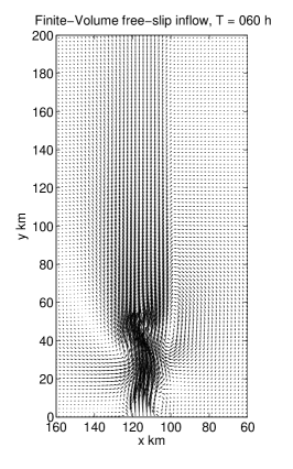
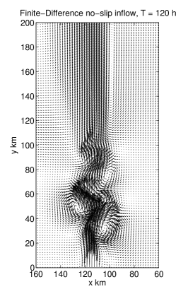
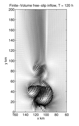
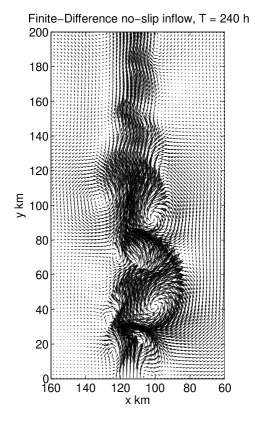
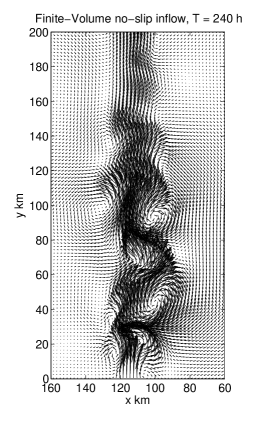
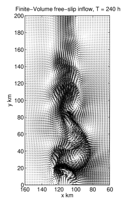
Figure 8. Ormen Lange Experiment I. Velocity plots at $60$ (top), $120$, and $240$ (bottom) hours, computed with the Finite-Difference scheme no-slip boundary condition (left), Finite-Volume no-slip boundary condition and Finite-Volume free-slip boundary condition (right).

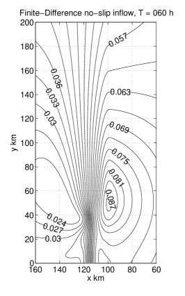
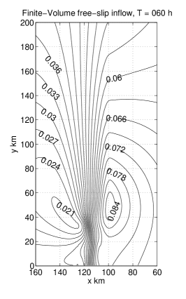
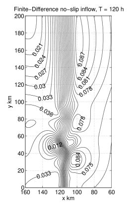
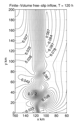
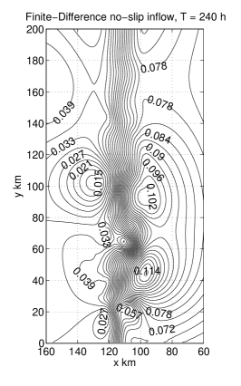
Figure 9. Ormen Lange Experiment I. Contour plots of surface elevation at $60$ (top), $120$, and $240$ (bottom) hours, computed with the Finite-Difference scheme no-slip boundary condition (left), Finite-Volume no-slip boundary condition and Finite-Volume free-slip boundary condition (right).

4.4.2. Setup for Ormen Lange Shelf Experiment II

In the setup of Section 4.4.1, the in-flowing jet was cut off at $x=L_{B}\pm B/2$. After some time, these points become transition points with a noticeable discontinuous shear layer. For the next experiment we avoid such a discontinuous shear layer and change the boundary condition by assigning the in-flowing jet profile $v_{jet}$ defined in equation (41) on the whole southern boundary.

The results are displayed in Figures 10. Eddies are still created and are of similar strength as in the previous section Figures 8. Note, however, that the maximal water level is now about 15cm, which is 3.3cm higher than before (11.7cm). This was to be expected because our new southern boundary condition does not allow any outflow.

From this experiment we can conclude that the non-smooth patching of the boundary condition at the southern boundary is not the mechanism which creates the instability. In the next experiment we will investigate if the instability is effected by the start-up procedure.

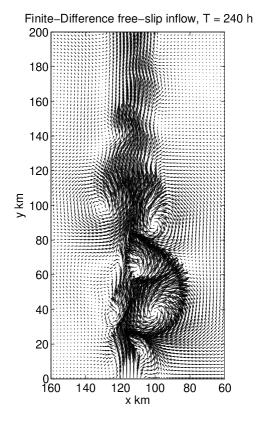
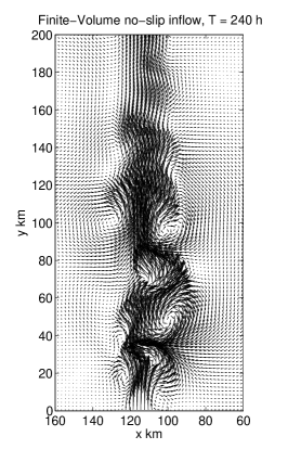
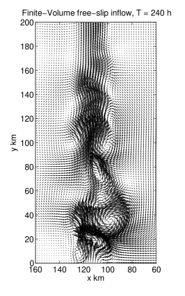
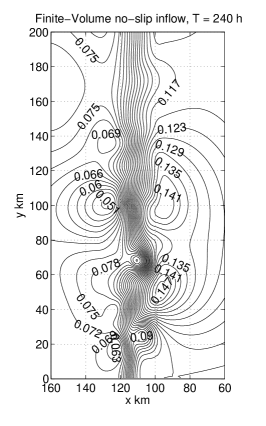
Figure 10. Ormen Lange Experiment II.. Contour plots of surface elevation (top) and velocity plots (bottom) at $240$ hours, computed with the Finite-Difference scheme free-slip boundary condition (left), Finite-Volume no-slip boundary condition and Finite-Volume free-slip boundary condition (right).

4.4.3. Setup for Ormen Lange Shelf Experiment III

We use the same setup as in Subsection 4.4.2 but here we use the smooth (four times continuously differentiable) growth function $\gamma(\tau)$ of (39) with $\tau=t/24h$, see Figure 11.

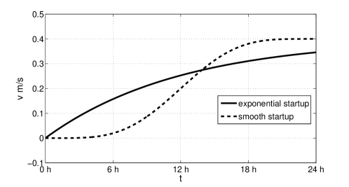
Figure 11. Smooth startup function $\gamma(\tau)$ compared with exponential startup.

Eddies are still being created and are qualitatively about the same as before. This is also suggested by the linear stability analysis in [9].

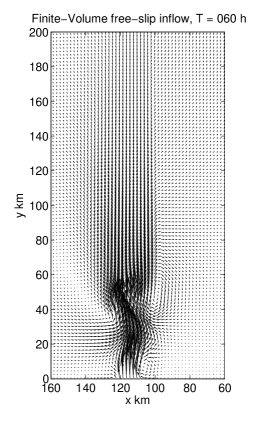
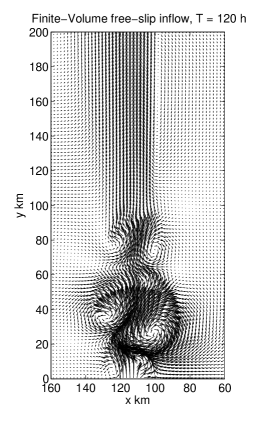
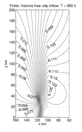
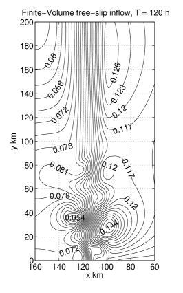
Figure 12. Ormen Lange Experiment III. Contour plots of surface elevation (top) and velocity plots (bottom) at $60$ (left), $120$, and $240$ (right) hours, computed with the Finite-Volume scheme free-slip boundary condition and smooth growth function Equation (39).

4.4.4. Setup for Ormen Lange Shelf Experiment IV

Here we present another variant of the southern boundary condition. In Section 4.4.1 we used a discontinuous patch of an in-flowing jet in the centre and open outflow at the periphery. In Section 4.4.2 we prescribed inflow everywhere. Now we joint the inflow- and the open outflow boundary conditions smoothly: Let $F_{i+\frac{1}{2},j}^{infl}$ be the flux determined by the free-slip inflow boundary condition and $F_{i+\frac{1}{2},j}^{absorb}$ the one given by the absorbing outflow boundary condition. Now we use the following convex combination to obtain the effective boundary flux

(44) $$F_{i+\frac{1}{2},j}:=\chi(x)F_{i+\frac{1}{2},j}^{infl}+(1-\chi(x))F_{i+\frac{1}{2},j}^{absorb}.$$

The function $\chi(x)$, which prescribes the transition from the open outer region towards the jet in the centre of the domain, is given by

$$\chi(x)=\left\{\begin{array}[]{ll}0&,x<T_{W}-R,\\ \Theta\left(\frac{x-T_{W}+R)}{2R}\right)&,T_{W}-R\leq x\leq T_{W}+R,\\ 1&,T_{W}+R<x<T_{E}-R,\\ \Theta\left(\frac{2R-(x-T_{E}+R)}{2R}\right)&,T_{E}-R\leq x\leq T_{E}+R,\\ 0&,x>T_{E}+R.\end{array}\right.$$

Here $\Theta(x):=x^{5}\left[126+x(-420+x(540+x(-315+70x)))\right]$ and the smoothing radius is $R=5000$. The transition points are $T_{W}:=L_{B}-\frac{1}{2}B$ and $T_{E}:=L_{B}+\frac{1}{2}B$.

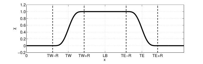
Figure 13. The function $\chi(x)$ prescribes the convex combination of the absorbing condition and the jet

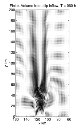
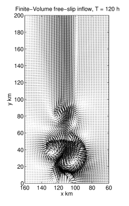
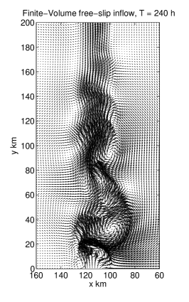
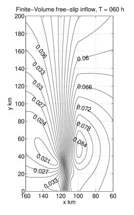
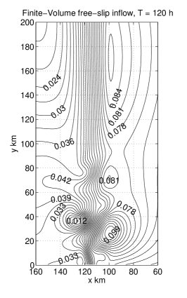
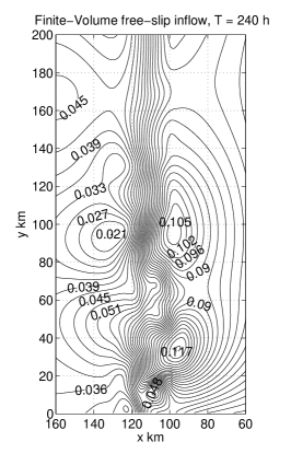
Figure 14. Ormen Lange Experiment IV. Contour plots of surface elevation (top) and velocity plots (bottom) at $60$ (left), $120$, and $240$ (right) hours, computed with the Finite-Volume scheme free-slip boundary condition and exponential growth function Equation (39) and transition smoothing.

The numerical results are shown in Figure 14. They agree in considerable detail with the previous computations and hence confirm the development of eddies, without introducing any discontinuity via the numerical boundary treatment.

4.4.5. Balanced inflow boundary conditions: Ormen Lange Shelf Experiment V

There remains one technical issue concerning the previous boundary condition: the transition points $T_{E}$ and $T_{W}$ have to be chosen by hand. This is not necessary for the volume-flux balanced boundary condition derived in Section  3.2.4 . There the decision of outflow/inflow is taken automatically by the Riemann solver.

The results for the balanced boundary condition are shown in Figure 19. They are in excellent agreement with the results in Figure 14. This shows that the volume-flux boundary condition is an interesting alternative to the previous treatments, if we know the far-field values $\eta(x_{0},y_{0})$ and $U(x_{0},y_{0})$. The results for the geostrophically balanced boundary condition are almost identical, and hence we do not display them here.

4.4.6. Comparison with linear stability analysis

Linear stability analysis described in [8] and [26] shows that the along shelf jet as defined for the Ormen Lange case, section 4.4.1, is unstable with respect to along shelf wave perturbations. The maximum predicted exponential growth rate of $0.44$ day^-1 occurs for a wave length of $44$ km. The corresponding wave period is $34.2$ hours. A second unstable mode has a maximum growth rate of $0.28$ day^-1, a wave length of $54$ km and a period of $41.1$ hours. There are also steady, neutrally stable, shelf wave oscillations in the band of wave lengths around $1000-1200$ km with corresponding period $35.6-40.5$ hours.

To compare the results of the linear stability analysis with the solution of the finite volume scheme in more detail we did the same computation as in section 4.4.1 on an enlarged domain of $300\times 9600\textnormal{km}^{2}$, grid-width $2$ km and final time $480$ hours (see Figure 15). Since several periods of the long waves (wavelength $1000-1200$ km) fit into this domain, it is possible to measure the wavelength very accurately.

Figure 15. Large domain of $300\times 9600$ km², where the two cross-sections from Figure 16 and Figure 17 are marked, the position from which the frequency plots Figure 18 are taken is marked with the black circle.

Figure 16 shows the surface elevation for the section $x=100$ km, $0$ km $\leq y\leq 400$ km, which is the upper shelf-edge. It is here that we observe the strongest wave amplitudes. The peaks indicate a wave length of $49$ km, which is the distance of the eddies.

Figure 16.

Section of surface displacement at $x=100$ km, computed on a domain of $300\times 9600$ km². The maximum exponential growth rate is observed for a wave length of $49$ km.

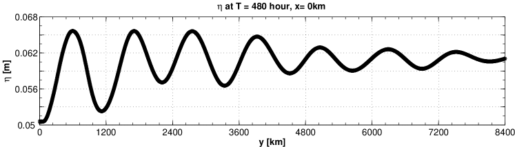
Figure 17. .The wave length of the neutrally stable long- wave at the eastern boundary $x=0$ km is $1152$ km.

Figure 17 shows the surface elevation for the section along the coast ($x=0$ km, $0$ km $\leq y\leq 8400$ km). Here we observe the second strongest wave amplitudes. The peaks indicate a wave length of $1152$ km. Both wave, the one in Figure 16 with wave length $49$ km, and the one in Figure 17 with $1152$ km, have the same wave period of $39.5$ hours. For the second wave, time-plots of surface displacement, and velocity $v$ are shown in Figure 18. Time plots for the first wave are similar, and not shown here.

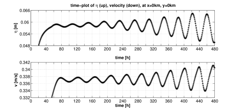
Figure 18. The frequency of the maximum unstable waves is approximately $39.5$ hour. The upper plot shows the frequency in the surface displacement and the lower plot shows the the frequency in normal velocity $v$.

The computational results of Figure 16, showing the development of eddies with period $35-40$ hours and an along shelf separation of $40-60$ km, are in close, but not complete, agreement with the predictions of the linear stability analysis.

The oscillation with wave length of about $1200$ km and period about $40$ hours (see Figure 17) is most pronounced in the sea level $\eta$ and its amplitude grows considerably over a time span of $10$ days. Clearly, this oscillation corresponds to the steady long shelf wave oscillations found by the stability analysis. In the numerical simulations the oscillation seems to be excited by the periodic eddy formation near the inflow boundary and propagates subsequently downstream with a speed of about $30$ km/hours.

A perfect correspondence between the linear stability analysis and the numerical simulations of the inflow jet cannot be expected due to nonlinear effects and the downstream development of the eddies in the model.

Note that for the situations computed above, the finite difference scheme yields almost equal results as the finite volume scheme.

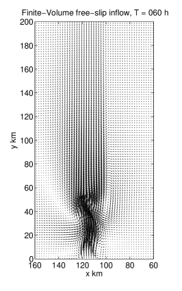
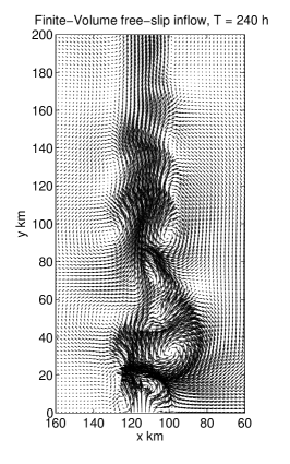
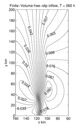
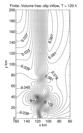
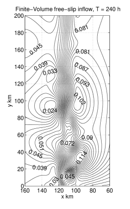
Figure 19. Ormen Lange Experiment VI. Contour plots of surface elevation (top) and velocity plots (bottom) at $60$ (left), $120$, and $240$ (right) hours, computed with the Finite-Volume scheme free-slip boundary condition, exponential growth function and balanced Equation (30) at inflow.

5. Conclusion

In this paper we have presented a comparison of a finite-difference and a high-order finite-volume scheme for geophysical flow problems. To conclude our report we discuss

1. the efficiency and stability of the FD and FV solvers,

2. the numerical inflow boundary conditions,

3. the geophysical implication of the computational results.

5.1. Efficiency and stability of the FD and FV solvers

The results indicate that the two schemes compute qualitatively and quantitatively similar solutions. The rates of convergence are as expected, i.e., first order for the original finite-difference scheme used by Gjevik et al. in [9], second order for the modified finite-difference scheme, and fourth order (almost fifth) for the finite-volume scheme.

An exact quantitative comparison of run-times is not possible, since the two codes are research codes written in different languages and by different programmers. However, it is fair to say that for the very smooth test problems 4.1 (see Table 2 and Table 3) and 4.2 the higher order finite volume scheme is asymptotically more efficient. For the more realistic, and less smooth, test problems Section 4.4, both the FD and the FV code give qualitatively the same results on the same grid, but the FD scheme is much faster than the FV scheme. It would be desirable to run the FV scheme on a coarser grid to reduce the runtime. But then the inflow data for the jet would be resolved by less then 10 cells, and the flow is not sufficiently resolved any more. This might be different for broader currents. Note that the FV scheme could resolve small gravity waves which were completely smeared by the FD scheme. However, these waves quickly leave the computational domain and do not seem to have a noticeable impact on the major currents.

But the FV scheme has an important advantage over the FD scheme: it is much more stable in cases with strong gradient. We can run it with CFL numbers of 0.5 (in all our computations) and sometimes up to 1, without adding any artificial viscosity. This includes solutions with shock-like discontinuities, e.g. hydraulic jumps. If we run the FD scheme without artificial viscosity, and for smooth solutions, it may already produce instabilities for CFL numbers of 0.5. This happened for example when we implemented the free-slip boundary condition into the FD scheme. For hydraulic jumps, a lot of artificial viscosity has to be added to stabilise the FD scheme, and this reduces the accuracy of the scheme.

5.2. Numerical inflow boundary conditions

Using Riemann decompositions, we could successfully translate the FD boundary conditions to the FV solver. We could also improve the no-slip inflow boundary conditions by the free-slip condition, which yields smoother solutions (Tables 4-7). Moreover, we developed a transparent inflow condition, which allows waves to leave the domain through the inflow boundary.

5.3. Geophysical implication of the computational results

Various numerical experiments for the Ormen Lange cases presented in Section 4.4, with the FD and the FV schemes and different implementations of the boundary conditions led to almost identical results for two different startup profile configurations. These results are also in close agreement with linear stability analysis (see Section 4.4.6). Therefore the computations presented here fully confirm the results of [26] about instabilities of the shelf slope jet and the formation of eddies.

5.4. Further perspectives

The finite-volume scheme is much more expensive with respect with computer time than the traditional finite-difference scheme, but one benefit from a lot higher accuracy. To obtain a similar accuracy with the finite-difference scheme one would have to refine the grid several times. This may make the finite-volume scheme attractive for studies of high frequency oscillations associated with strong current shears or small scale bathymetric features on the shelf edge.

References

- [1] E. Audusse, F. Bouchut, M.-O. Bristeau, R. Klein, B. Perthame. A fast and stable well-balanced scheme with hydrostatic reconstruction for shallow water flows. SIAM J. Sci. Comp. 25, (2004), 2050–2065.
- [2] F. Bouchut, J. Le Sommer and V. Zeitlin. Frontal geostrophic adjustment and nonlinear-wave phenomena in one dimensional rotating shallow water. Part 2: high-resolution numerical simulations. J. Fluid Mech. 514 (2004), 35–63.
- [3] A.F. Benette, P.E. Kloeden. The Ill-Posedness of open Ocean Models. J. Phys. Oceanogr. (1981), 1027–1029.
- [4] D. G. Dritschel, L. M. Polvani and A. R. Mohebalhojeh. The contour-advective semi-Lagrangian algorithm for the shallow water equations. Monthly Weather Review, 127 (1999), 1551–1565.
- [5] N.A. Edwards, C.P.Please and R.W. Preston. Some Observations on Boundary Conditions for the Shallow-water Equations in Two Space Dimensions. IMA Journal of Applied Mathematics Vol. 30, (1983), 161–172.
- [6] B. Engquist and A. Majda. Absorbing Boundary Conditions for the Numerical Simulation of Waves. Mathematics of Computation Vol. 31, Number 139 (1977), 629–651.
- [7] R.A. Flather. A tidal model of the northwest European continantal shelf. Memoires de la Societe Royale des Sciences de Liege 6 (1976), 141–164.
- [8] B. Gjevik. Unstable and neutrally stable modes in barotropic and baroclinic shelf slope currents. Preprint Series, Dept. of Math., Univ. of Oslo, No 1.
- [9] B. Gjevik, H. Moe and A. Ommundsen. Idealized model simulations of barotropic flow on the Catalan shelf. Continental Shelf Research Vol. 22 (2002), 173–198.
- [10] S.K. Godunov. A difference method for numerical calculation of discontinuous solutions of the equations of hydrodynamics. (Russian) Mat. Sb. (N.S.) Vol. 47 (1959), 271–306.
- [11] A. Harten. High resolution schemes for hyperbolic conservation laws. J. Comput. Phys. 49 (1983), no. 3, 357–393.
- [12] D. Kröner. Absorbing Boundary Conditions for the Linearized Euler Equations in 2-D. Mathematics of Computation Vol. 57, Number 195 (1991), 153–167.
- [13] P.D. Lax. Weak solutions of nonlinear hyperbolic equations and their numerical computation. Comm. Pure Appl. Math. 7, (1954). 159–193.
- [14] B. van Leer. Towards the ultimate conservative difference scheme. V. A second-order sequel to Godunov’s method. J. Comput. Phys. 32 (1979), 101–136.
- [15] R.J. LeVeque. Numerical methods for conservation laws. Second edition. Lectures in Mathematics ETH Zürich. Birkhäuser Verlag, Basel, (1992), ISBN: 3-7643-2723-5.
- [16] Lukacova . Well. J. Comput. Phys. 32 (2006), 101–136.
- [17] J. von Neumann and R.D. Richtmyer. A method for the numerical calculation of hydrodynamic shocks. J. Appl. Phys. 21, (1950). 232–237.
- [18] S. Noelle, N. Pankratz, G. Puppo and J. R. Natvig. Well-balanced finite-volume schemes of arbitrary order of accuracy for shallow water flows. J. Comput. Phys. 213 (2006), 474–499.
- [19] J. Oliger and A. Sundstrøm. Theoretical and practical aspects of some initial boundary-value problems in fluid-dynamics. SIAM J.Appl.Math. 35(3) (1978), 419–446.
- [20] R.D. Richtmyer and K.W. Morton. Difference methods for initial-value problems. Second edition. Interscience Publishers John Wiley & Sons New York (1967).
- [21] P.L. Roe. Approximate Riemann solvers, parameter vectors, and difference schemes. J. Comp. Phys. 43 (1981), 357–372.
- [22] J. Shi, C. Hu, and C.-W. Shu. A technique of treating negative weights in WENO schemes. J. Comp. Phys. 175 (2002), 108–127.
- [23] C.-W. Shu. Total-variation-diminishing time discretization. SIAM J.Sci.Statist.Comp. 9 (1988), 1073–1084.
- [24] C.-W. Shu. Essentially non-oscillatory and weighted essentially non-oscillatory schemes for hyperbolic conservation laws. in Advanced Numerical Approximation of Nonlinear Hyperbolic Equations, edited by B. Cockburn, C. Johnson, C.W. Shu and E. Tadmor, Lecture Notes in Mathematics, Springer-Verlag, Berlin/New York (1998), 325–432.
- [25] J. Smagorinsky. General circulation experiments with the primitive equation. Monthly Weather Review 91 (1) (1963), 99–164.
- [26] Ø. Thiem, J. Berntsen and B. Gjevik. Development of edddies in an idealized shelf slope area due to an along slope barostraophic jet. Continental Shelf Research Vol. 26 (2006), 1481–1495.
- [27] Y. Xing and C.-W. Shu. High Order Finite Difference WENO Schemes with the Exact Conservation Property for the Shallow Water Equations. J. Comp. Phys. Vol. 208 (2005), 206–227.