A well-balanced reconstruction of wet/dry fronts for the shallow water equations
Abstract
In this paper, we construct a well-balanced, positivity preserving finite volume scheme for the shallow water equations based on a continuous, piecewise linear discretization of the bottom topography. The main new technique is a special reconstruction of the flow variables in wet-dry cells, which is presented in this paper for the one dimensional case. We realize the new reconstruction in the framework of the second-order semi-discrete central-upwind scheme from (A. Kurganov and G. Petrova, Commun. Math. Sci., 2007). The positivity of the computed water height is ensured following (A. Bollermann, S. Noelle and M. Lukáčová, Commun. Comput. Phys., 2010): The outgoing fluxes are limited in case of draining cells.
keywords:
Hyperbolic systems of conservation and balance laws, Saint-Venant system of shallow water equations, finite volume methods, well-balanced schemes, positivity preserving schemes, wet/dry fronts. AMS subject classifications. 76M12, 35L651 Introduction
We study numerical methods for the Saint-Venant system of shallow water equations [3], which is widely used for the flow of water in rivers or in the ocean. In one dimension, the Saint-Venant system reads:
| (1.3) |
subject to the initial conditions
where is the fluid depth, is the velocity, is the gravitational constant, and the function represents the bottom topography, which is assumed to be independent of time and possibly discontinuous. The systems (1.3) is considered in a certain spatial domain and if the Saint-Venant system must be augmented with proper boundary conditions.
In many applications, quasi steady solutions of the system (1.3) are to be captured using a (practically affordable) coarse grid. In such a situation, small perturbations of steady states may be amplified by the scheme and the so-called numerical storm can spontaneously develop [19]. To prevent it, one has to develop a well-balanced scheme—a scheme that is capable of exactly balancing the flux and source terms so that “lake at rest” steady states,
| (1.4) |
are preserved within the machine accuracy. Here, denotes the total water height or free surface. Examples of such schemes can be found in [1, 2, 4, 5, 8, 9, 11, 12, 14, 13, 19, 20, 21, 22, 23, 30, 31].
Another difficulty one often has to face in practice is related to the presence of dry areas (island, shore) in the computational domain. As the eigenvalues of the Jacobian of the fluxes in (1.3) are , the system (1.3) will not be strictly hyperbolic in the dry areas (), and if due to numerical oscillations becomes negative, the calculation will simply break down. It is thus crucial for a good scheme to preserve the positivity of (positivity preserving schemes can be found, e.g., in [1, 4, 2, 11, 12, 20, 21]).
We would also like to point out that when the “lake at rest” steady state (1.4) reduces to
| (1.5) |
which can be viewed as a “dry lake”. A good numerical scheme may be considered “truly” well-balanced when it is capable of exactly preserving both “lake at rest” and “dry lake” steady states, as well as their combinations corresponding to the situations, in which the domain is split into two nonoverlapping parts (wet area) and (dry area) and the solution satisfies (1.4) in and (1.5) in .
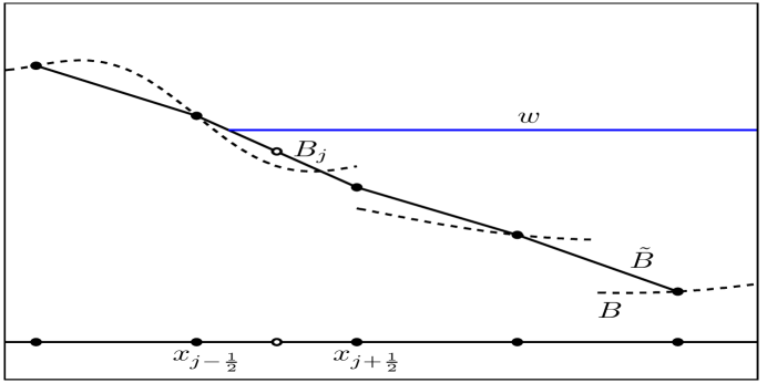
We focus on Godunov-type schemes, in which a numerical solution realized at a certain time level by a global (in space) piecewise polynomial reconstruction, is evolved to the next time level using the integral form of the system of balance laws. In order to design a well-balanced scheme for (1.3), it is necessary that this reconstruction respects both the “lake at rest” (1.4) and “dry lake” (1.5) steady-state solutions as well as their combinations. On the other hand, to preserve positivity we have to make sure that the reconstruction preserves a positive water height for all reconstructed values. Both of this has been achieved by the hydrostatic reconstruction introduced by Audusse et al. [1], based on a discontinuous, piecewise smooth discretisation of the bottom topography. In this paper, we consider a continuous, piecewise linear reconstruction of the bottom. We propose a piecewise linear reconstruction of the flow variables that also leads to a well-balanced, positivity preserving scheme. The new reconstruction is based on the proper discretization of a front cell in the situation like the one depicted in Figure 1. The picture depicts the real situation with a sloping shore, and we see a discretization of the same situation that seems to be the most suitable from a numerical perspective. We also demonstrate that the correct handling of (1.4), (1.5) and their combinations leads to a proper treatment of non-steady states as well.
Provided the reconstruction preserves positivity, we can prove that the resulting central-upwind scheme is positivity preserving. In fact, the proof from [12] carries over to the new scheme, but with a possibly severe time step constraint. We therefore adopt a technique from [2] and limit outgoing fluxes whenever the so-called local draining time is smaller than the global time step. This approach ensures positive water heights without a reduction of the global time step.
The paper is organized as follows. In §2, we briefly review the well-balanced positivity preserving central-upwind scheme from [12]. A new positivity preserving reconstruction is presented in §3. The well-balancing and positivity preserving properties properties of the new scheme are proven in §4. Finally, we demonstrate the performance of the proposed method in §5.
2 A Central-Upwind Scheme for the Shallow Water Equations
Our work will be based on the central-upwind scheme proposed in [12]. We will therefore begin with a brief overview of the original scheme.
We introduce a uniform grid , with finite volume cells of length and denote by the cell averages of the solution of (1.3) computed at time :
| (2.6) |
We then replace the bottom function with its continuous, piecewise linear approximation . To this end, we first define
| (2.7) |
which in case of a continuous function reduces to , and then interpolate between these points to obtain
| (2.8) |
From (2.8), we obviously have
| (2.9) |
The central-upwind semi-discretization of (1.3) can be written as the following system of time-dependent ODEs:
| (2.10) |
where are the central-upwind numerical fluxes and is an appropriate discretization of the cell averages of the source term:
| (2.11) |
Using the definitions (2.7) and (2.9), we write the second component of the discretized source term (2.11) as (see [11] and [12] for details)
| (2.12) |
The central-upwind numerical fluxes are given by:
| (2.13) | |||||
where we use the following flux notation:
| (2.14) |
The values represent the left and right values of the solution at point obtained by a piecewise linear reconstruction
| (2.15) |
of standing for and respectively with . To avoid the cancellation problem near dry areas, we define the average velocity by
We choose in all of our numerical experiments. This reconstruction will be second-order accurate if the approximate values of the derivatives are at least first-order approximations of the corresponding exact derivatives. To ensure a non-oscillatory nature of the reconstruction (2.15) and thus to avoid spurious oscillations in the numerical solution, one has to evaluate using a nonlinear limiter. From the large selection of the limiters readily available in the literature (see, e.g., [6, 10, 29, 13, 16, 18, 25]), we chose the generalized minmod limiter ([29, 16, 18, 25]):
| (2.16) |
where the minmod function, defined as
| (2.17) |
is applied in a componentwise manner, and is a parameter affecting the numerical viscosity of the scheme. It is shown in [12] that this procedure (as well as any alternative “conventional” reconstruction, including the simplest first-order piecewise constant one, for which ) might produce negative values near the dry areas (see [12]). Therefore, the reconstruction (2.15)–(2.17) must be corrected there. The correction algorithm used in [12] restores positivity of the reconstruction depicted in Figure 3, but destroys the well-balancing property. This is explained in §3, where we propose an alternative positivity preserving reconstruction, which is capable of exactly preserving the “lake at rest” and the “dry lake” steady states as well as their combinations.
Finally, the local speeds in (2.13) are obtained using the eigenvalues of the Jacobian as follows:
| (2.18) | ||||
| (2.19) |
Note that for , and , we dropped the dependence of for simplicity.
As in [12], in our numerical experiments, we use the third-order strong stability preserving Runge-Kutta (SSP-RK) ODE solver (see [7] for details) to numerically integrate the ODE system (2.10). The timestep is restricted by the standard CFL condition,
| (2.20) |
For the examples of the present paper, results of the second and third order SSP-RK solvers are almost undistinguishable.
3 A New Reconstruction at the Almost Dry Cells
In the presence of dry areas, the central-upwind scheme described in the previous section may create negative water depth values at the reconstruction stage. To understand this, one may look at Figure 2, where we illustrate the following situation: The solution satisfies (1.4) for (where marks the waterline) and (1.5) for . Notice that cell is a typical almost dry cell and the use of the (first-order) piecewise constant reconstruction clearly leads to appearance of negative water depth values there. Indeed, in this cell the total amount of water is positive and therefore , but clearly and thus .
It is clear that replacement of the first-order piecewise constant reconstruction with a conventional second-order piecewise linear one will not guarantee positivity of the computed point values of . Therefore, the reconstruction in cell may need to be corrected. The correction proposed in [12] will solve the positivity problem by raising the water level at one of the cell edges to the level of the bottom function there and lowering the water level at the other edge by the same value (this procedure would thus preserve the amount of water in cell ). The resulting linear piece is shown in Figure 3. Unfortunately, as one may clearly see in the same figure, the obtained reconstruction is not well-balanced since the reconstructed values and are not the same.
Here, we propose an alternative correction procedure, which will be both positivity preserving and well-balanced even in the presence of dry areas. This correction bears some similarity to the reconstruction near dry fronts of depth-averaged granular avalanche models in [28]. However, in [28] the authors tracked a front running down the terrain, and did not treat well-balancing of equilibrium states. Let us assume that at a certain time level all computed values and the slopes and in the piecewise linear reconstruction (2.15) have been computed using some nonlinear limiter as it was discussed in §2 above. We also assume that at some almost dry cell ,
| (3.21) |
(the case can obviously be treated in a symmetric way) and that the reconstructed values of in cell satisfy
| (3.22) |
that is, cell is fully flooded. This means that cell is located near the dry boundary (mounting shore), and we design a well-balanced reconstruction correction procedure for cell in the following way:
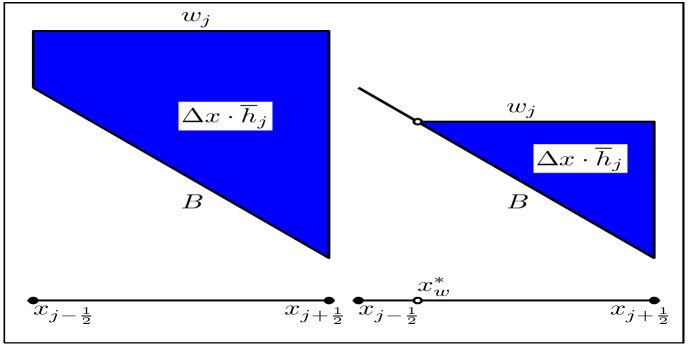
We begin by computing the free surface in cell (denoted by ), which represents the average total water level in (the flooded parts of) this cell assuming that the water is at rest. The meaning of this formulation becomes clear from Figure 4. We always choose such that the area enclosed between the line with height and the bottom line equals the amount of water given by , where . The resulting area is either a trapezoid (if cell is a fully flooded cell as in Figure 4 on the left) or a triangle (if cell is a partially flooded cell as in Figure 4 on the right), depending on and the bottom slope .
So if the cell is a fully flooded cell, i.e. , the free surface is defined as
otherwise the free surface is a continuous piecewise linear function given by
| (3.23) |
where is the boundary point separating the dry and wet parts in the cell . It can be determined by the mass conservation,
where , thus
| (3.24) |
resulting in the free surface formula for the wet/dry cells,
| (3.25) |
Note that the limit for the distinction of cases in (3.23) is determined from the area of the triangle between the bottom line and the horizontal line at the level of . We also note that if cell satisfies (3.21), then it is clearly a partially flooded cell (like the one shown in Figure 4 on the right) with .
Remark 3.1
We would like to emphasize that if cell is fully flooded, then the free surface is represented by the cell average (see the first case in equation (3.23)), while if the cell is only partially flooded, does not represent the free surface at all (see, e.g., Figure 2). Thus, in the latter case we need to represent the free surface with the help of another variable (see the second case in (3.23)), which is only defined on the wet part of cell , , and thus stays above the bottom function , see Figure 4 (right).
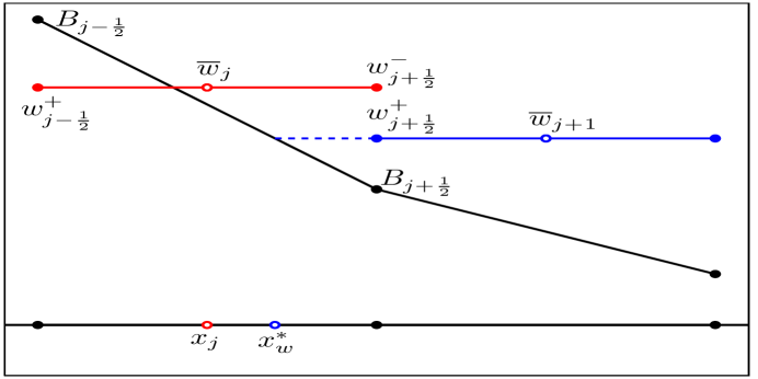
We now modify the reconstruction of in the partially flooded cell to ensure the well-balanced property. To this end, we first set (which immediately implies that ) and determine the reconstruction of in cell via the conservation of in this cell. We distinguish between the following two possible cases. If the amount of water in cell is sufficiently large (as in the case illustrated in Figure 5 on the left), there is a unique satisfying
| (3.26) |
From this we obtain , and thus the well-balanced reconstruction in cell is completed.
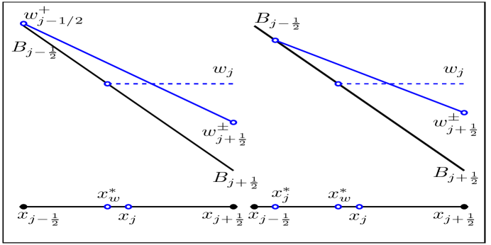
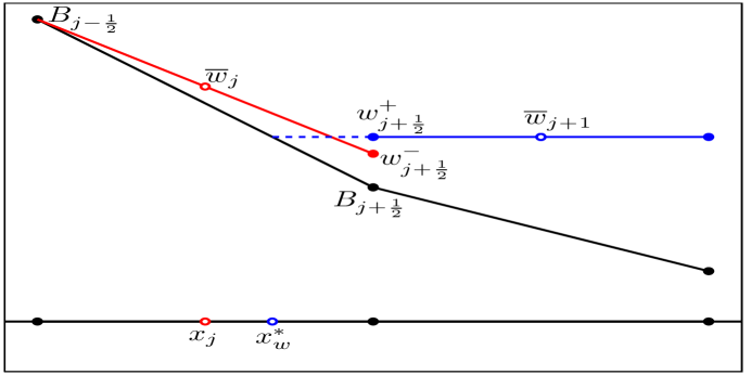
If the value of , computed from the conservation requirement (3.26) is negative, we replace a linear piece of in cell with two linear pieces as shown in Figure 5 on the right. The breaking point between the “wet” and “dry” pieces will be denoted by and it will be determined from the conservation requirement, which in this case reads
| (3.27) |
where
Combining the above two cases, we obtain the reconstructed value
| (3.28) |
We also generalize the definition of and set
| (3.29) |
which will be used in the proofs of the positivity and well-balancing of the resulting central-upwind scheme in §4. We summarize the wet/dry reconstruction in the following definition:
Definition 3.2
(wet/dry reconstruction) For the sake of clarity, we denote the left and right values of the piecewise linear reconstruction (2.15) – (2.17) by . The purpose of this definition is to define the final values , which are modified by the wet/dry reconstruction.
- Case 1.
-
and : there is enough water to flood the cell for flat lake.
- 1A.
-
and : the cell is fully flooded, and we set .
- 1B.
- Case 2.
-
: the cell is possible partially flooded.
- 2A.
-
and , i.e., cell is fully flooded and . Define and .
- 2A1.
-
, the amount of water in cell is sufficiently large, we set , so
- 2A2.
-
otherwise set and as in (3.29).
- 2B.
- Case 3.
-
: analogous to Case 2.
4 Positivity Preserving and Well-Balancing
In the previous section, we proposed a new spatial reconstruction for wet/dry cell. In this section, we will implement a time-quadrature for the fluxes at wet/dry boundaries developed in [2]. It cuts off the space-time flux integrals for partially flooded interfaces. Then we prove that the resulting central-upwind scheme is positivity preserving and well-balanced under the standard CFL condition (2.20).
We begin by studying the positivity using a standard time integration of the fluxes. The following lemma shows that for explicit Euler time stepping, positivity cannot be guaranteed directly under a CFL condition such as (2.20).
Lemma 4.1
(2.10)–(2.19) with the piecewise linear reconstruction
(2.15) corrected according to the procedure described in
§3. Assume that the system of ODEs (2.10) is solved by
the forward Euler method and that for all , . Then
(i) for all provided that
| (4.30) |
(ii) Condition (4.30) cannot be guaranteed by any finite positive CFL condition (2.20).
Proof: (i) For the fully flooded cells with , the proof of Theorem 2.1 in [12] still holds. Therefore, we will only consider partially flooded cells like the one shown in Figure 5. First, from (3.27) we have that in such a cell the cell average of the water depth at time level is
| (4.31) |
and it is evolved to the next time level by applying the forward Euler temporal discretization to the first component of (2.10), which after the subtraction of the value from both sides can be written as
| (4.32) |
where the numerical fluxes are evaluated at time level . Using (2.13) and the fact that by construction , we obtain:
| (4.33) |
Substituting (4.31) and (4.33) into (4.32) and taking into account the fact that in this cell , we arrive at:
| (4.34) | |||||
Next, we argue as in [12, Theorem 2.1] and show that is a linear combination of the three values, and (which are guaranteed to be nonnegative by our special reconstruction procedure) with nonnegative coefficients. To this end, we note that it follows from (2.18) and (2.19) that , , , and , and hence the last two terms in (4.34) are nonnegative. By the same argument, and , and thus the first term in (4.34) will be also nonnegative, provided the CFL restriction (4.30) is satisfied. Therefore, , and part (i) is proved.
In order to show part (ii) of the lemma, we compare the CFL-like conndition (4.30) with the standard CFL condition (2.20),
| (4.35) |
We note that depending on the water level in the partially flooded cell, can be arbitrarily small, so there is no upper bound of in terms of .
Part (ii) of Lemma 4.1 reveals that one might obtain a serious restriction of the timestep in the presence of partially flooded cells. We will now show how to overcome this restriction using the draining time technique developed in [2].
We start from the equation (4.32) for the water height and look for a suitable modification of the update such that the water height remains positive,
As in [2], we introduce the draining time step
| (4.36) |
which describes the time when the water contained in cell in the beginning of the time step has left via the outflow fluxes. We now replace the evolution step (4.32) with
| (4.37) |
where we set the effective time step on the cell interface as
| (4.38) |
The definition of selects the cell in upwind direction of the edge. We would like to point out that the modification of flux is only active in cells which are at risk of running empty during the next time step. It corresponds to the simple fact that there is no flux out of a cell once the cell is empty. The positivity based on the draining time is summarized as the following theorem, which we proved in [2]. Note that in contrast to Lemma 4.1, the timestep is now uniform under the CFL condition (2.20):
Theorem 4.1.
To guarantee well-balancing, we have to make sure that the gravity driven part of the momentum flux cancels the source term , in a lake at rest situation. To this end, we follow [2] and split the momentum flux in its advective and gravity driven parts:
respectively. For convenience, we will denote by in the following. The corresponding advective and gravity driven parts of the central-upwind fluxes then read
and
The above fluxes adds up to the following modified update of the momentum:
| (4.40) |
This modified finite volume scheme (4.37) and (4.40) ensures the well-balancing property even in the presence of dry areas, as we will show in Theorem 4.2.
Theorem 4.2.
Consider the system (1.3) and the fully discrete central-upwind scheme (4.37) and (4.40). Assume that the numerical solution corresponds to the steady state which is a combination of the “lake at rest” (1.4) and “dry lake” (1.5) states in the sense that for all defined in 3.23, and whenever . Then , that is, the scheme is well-balanced.
Proof: We have to show that in all cells the fluxes and the source term discretization cancel exactly. First, we mention the fact that the reconstruction procedure derived in §3 preserves both the “lake at rest” and “dry lake” steady states and their combinations. For all cells where the original reconstruction is not corrected, the resulting slopes are obviously zero and therefore there. As in all cells, the reconstruction for obviously reproduces the constant point values , resulting that the draining time is equal to the global time step, i.e., .
We first analyze the update of the free surface using (4.37). The first component of flux (2.13) is
as , and . This gives
Secondly, we analyze the update of the momentum using (4.40). Using the same argument and setting at the points where , for the second component we obtain
where . So, the finite volume update (4.40) for the studied steady state reads after substituting the source quadrature (2.12),
where we have used
| (4.41) |
It remains the verify (4.41). In the fully flooded cells, where , we have
and thus (4.41) is satisfied. In the partially flooded cells (as the one shown in Figure 4 on the right), , , and thus using (3.27) equation (4.41) reduces to
which is true since at the studied-steady situation, , which implies that , and hence, .
This concludes the proof of the theorem.
Remark 2.
Remark 3.
We would like to point out that the resulting scheme will clearly remain positivity preserving if the forward Euler method in the discretization of the ODE system (2.10) is replaced with a higher-order SSP ODE solver (either the Runge-Kutta or the multistep one), because such solvers can be written as a convex combination of several forward Euler steps, see [7]. In each Runge-Kutta stage, the time step is chosen as the global time step at the first stage. This is because the draining time , which is a local cut-off to the numerical flux, does not reduce, or even influence, the global time step.
5 Numerical Experiments
To show the effects of our new reconstruction at the boundary, we first test the numerical accuracy order using a continuous problem; then compare our new scheme with the scheme from [12] for the oscillating lake problem and the wave run-up problem on a slopping shore. These schemes only differ in the treatment of the dry boundary, so that the effects of the proposed modifications are highlighted. At last, we apply our scheme to dam-break problems over a plane and a triangular hump with bottom friction. For the sake of brevity, we refer to the scheme from [12] as KP and to our new scheme as BCKN.
Before the simulations, let us talk about the cell averages for the initial condition. Suppose that the states at cell interfaces and are given. The cell averages of momentums are computed using the trapezoidal rule in the cells as
As for the water height, we have to distinguish between three cases [21]. Cells are called wet cells if the water heights at both cell interfaces are positive,
If instead,
we speak of cells with upward slope. If
we speak of downward slope. For the wet cells and cells with downward slope, the cell averages of water height are computed using the trapezoidal rule in the cells as
because it is impossible to be still water states. For the adverse slope, we use the inverse function of (3.25),
to computed the cell average water height assuming the water is flat. It is easy to see from our new reconstruction (3.24), (3.25) and (3.29) can exactly reconstruct the initial still water states.
5.1 Numerical accuracy order
To compute the numerical order of accuracy of our scheme, we choose a continuous example from [12]. With computational domain , the problem is subject to the gravitational constant , the bottom topography
the initial data
and the periodic boundary conditions.
| # points | error | EOC | error | EOC |
|---|---|---|---|---|
| 25 | 5.30e-2 | 2.33e-1 | ||
| 50 | 1.51e-2 | 1.81 | 1.38e-1 | 0.76 |
| 100 | 4.86e-3 | 1.63 | 4.43e-2 | 1.64 |
| 200 | 1.40e-3 | 1.80 | 1.14e-2 | 1.95 |
| 400 | 3.59e-4 | 1.96 | 2.84e-3 | 2.01 |
| 800 | 8.93e-5 | 2.01 | 7.05e-4 | 2.01 |
The reference solution is computed on a grid with cells. The numerical result is shown in the Table 1 at time . The result confirm that our scheme is second-order accurate.
5.2 Still and oscillating lakes
In this section, we consider present a test case proposed in [1]. It describes the situation where the “lake at rest” (1.4) and “dry lake” (1.5) are combined in the domain with the bottom topography given by
| (5.42) |
and the following initial data:
| (5.43) |
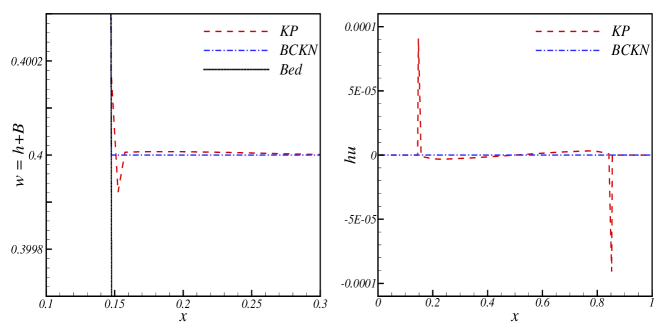
We compute the numerical solution by the KP and BCKN schemes with points at the final time . The results are shown in Figure 6 and Table 2. As one can clearly see there, the KP scheme introduces some oscillations at the boundary, whereas the BCKN scheme is perfectly well-balanced which means that our new initial data reconstruction method can exactly preserve the well-balanceed property not only in the wet region but also in the dry region. And the influence on the solutions away from the wet/dry front is also visible because of oscillations at the boundary produced by the KP schme.
| scheme | error of | error of |
|---|---|---|
| KP | 7.88e-5 | 9.08e-5 |
| BCKN | 3.33e-16 | 5.43e-16 |
We now consider a sinusoidal perturbation of the steady state (5.42), (5.43) by taking
As in [1], we set the final time to be . At this time, the wave has its maximal height at the left shore after some oscillations.
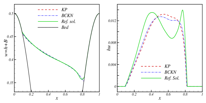
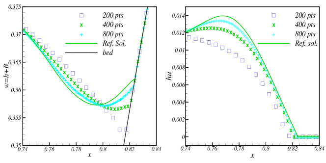
In Figure 7 we compare the results obtained by the BCKN and KP schemes with points with a reference solution (computed using points). Table 3 shows the experimental accuracy order for the two different schemes. One can clearly see that both KP and BCKN scheme can produce good results and acceptable numerical order. In Figure 8 we show a zoom of BCKN solutions for with 200, 400 and 800 points, which converge nicely to the reference solution. In particular, the discharge converges without any oscillations.
| # points | error | EOC | error | EOC |
|---|---|---|---|---|
| 25 | 9.48e-3 | 1.47e-2 | ||
| 50 | 2.81e-3 | 1.75 | 7.26e-3 | 1.02 |
| 100 | 1.65e-3 | 0.77 | 2.46e-3 | 1.56 |
| 200 | 7.88e-4 | 1.06 | 1.59e-3 | 0.63 |
| 400 | 3.33e-4 | 1.24 | 6.19e-4 | 1.36 |
| 800 | 1.26e-4 | 1.40 | 2.27e-4 | 1.45 |
| KP scheme | ||||
| 25 | 7.55e-3 | 1.31e-2 | ||
| 50 | 2.27e-3 | 1.74 | 6.04e-3 | 1.11 |
| 100 | 1.45e-3 | 0.65 | 2.35e-3 | 1.36 |
| 200 | 6.77e-4 | 1.09 | 1.31e-3 | 0.84 |
| 400 | 2.71e-4 | 1.32 | 5.04e-4 | 1.38 |
| 800 | 1.04e-4 | 1.38 | 1.87e-4 | 1.43 |
| BCKN scheme |
5.3 Wave run-up on a sloping shore
This test describes the run-up and reflection of a wave on a mounting slope. It was proposed in [27] and reference solutions can be found, for example, in [2, 21, 26].
The initial data are
and the bottom topography is
The computational domain is and the number of grid cells is .
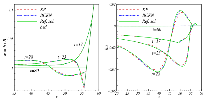
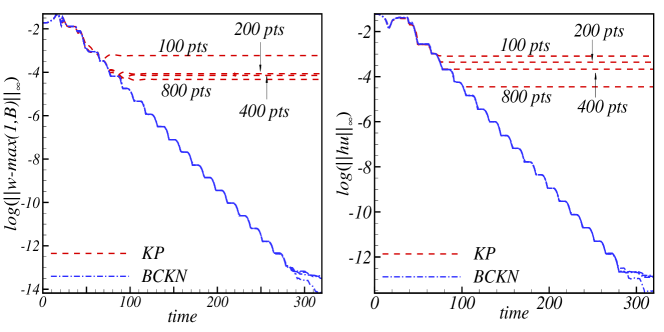
Figure 9 shows the free surface and discharge computed by both BCNK and KP schemes for different times. The reference solution is computed using 2000 points. A wave is running up the shore at time , and running down at . At time a steady state is reached. In the dynamic phase (up to time ), both schemes provide satisfactory solutions. In Figure 10 we study the long time decay towards equilibrium for different grid size resolutions. While the BCKN solutions decay up to machine accuracy, the long time convergence of the KP scheme comes to a halt. A brief check reveals that the deviation from equilibrium is roughly of the size of the truncation error of the KP scheme.
5.4 Dam-break over a plane
Here we study three dam breaks over inclined planes with various inclination angles. These test cases have been previously considered in [4, 32].
The domain is , the bottom topography is given by
where is the inclination angle. The initial data are
At we impose a free flow boundary condition, and at we set the discharge to zero. The plane is either flat (), inclined uphill (), or downhill ().
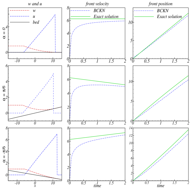
We run the simulation until time , with 200 uniform cells. The numerical results are displayed in Figure 11, for inclination angles , and , from top to bottom. The left column shows and , the central column the front position and the right column the front velocity. We also display the exact front positions and velocities (see [4]) given by
As suggested in [32], we define the numerical front position to be the first cell (counted from right to left) where the water height exceeds . While the BCKN scheme, which is only second order accurate, cannot fully match the resolution of the third and fifth order schemes in [4, 32], it still performs reasonably well. What we would like to stress here is that the new scheme, which was designed to be well balanced near wet/dry equilibrium states, is also robust for shocks running into dry areas.
5.5 Laboratory dam-break over a triangular hump
We apply our scheme to a laboratory test of a dam-break inundation over a triangular hump which is recommended by the Europe, the Concerted Action on Dam-Break Modeling (CADAM) project [17]. The problem consider the friction effect and then the corresponding governing equation (1.3) is changed to be
| (5.46) |
where represents the energy dissipation effect and are estimated from bed roughness on the flow, is the density of water and represents the bed roughness coefficient with being the Manning coefficient. For small water depths, the bed friction term dominates the other terms in the momentum equation, due to the presence of in the denominator. To simplify the update of the momentum, we first update the solution using our new positivity preserving and well-balanced scheme stated in section 2, 3 and 4 without the bed friction effect, and then retain the local acceleration from the only bed friction terms.
| (5.47) |
A partially implicit approach [15, 24] is used for the discretization of the above equation as
| (5.48) |
Resolving this for , we obtain
| (5.49) |
where and are given using our above stated scheme without friction term. The initial conditions and geometry (Figure 12) were identical to those used by [15, 24]. The experiment was conducted in a 38-m-long channel. The dam was located at 15.5 m, with a still water surface of 0.75 m in the reservoir. A symmetric triangular obstacle 6.0 m long and 0.4 m high was installed 13.0 m downstream of the dam. The floodplain was fixed and initially dry, with reflecting boundaries and a free outlet. The Manning coefficient was 0.0125, adopted from [15]. The flow depth was measured at seven stations, GP2, GP4, GP8, GP10, GP11, GP13, and GP20, respectively, located at 2, 4, 8, 10, 11, 13, and 20 m downstream of the dam, as shown in Figure 12. The simulation was conducted for 90 seconds.
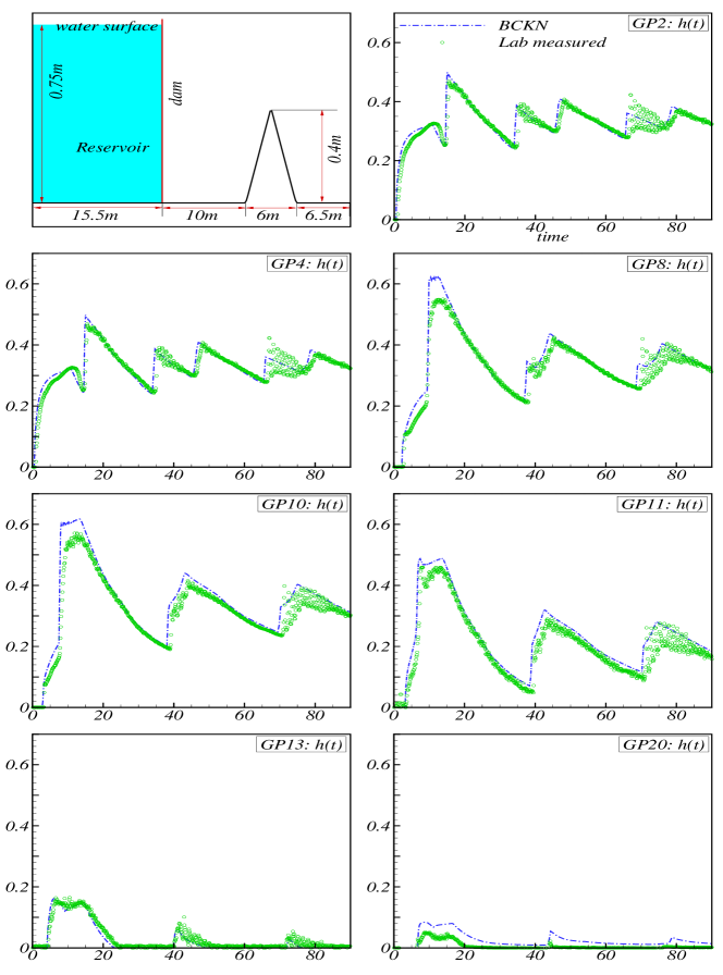
The numerical predictions using 200 points are shown in Figure 12. The comparison between the numerical results and measurements is satisfactory at all gauge points and the wet/dry transitions are resolved sharply (compare with [15, 24] and the references therein). This confirms the effectiveness of the current scheme together with the implicit method for discretization of the friction term, even near wet/dry fronts.
6 Conclusion
In this paper, we designed a special reconstruction of the water level at wet/dry fronts, in the framework of the second-order semi-discrete central-upwind scheme and a continuous, piecewise linear discretisation of the bottom topography. The proposed reconstruction is conservative, well-balanced and positivity preserving for both wet and dry cells. The positivity of the computed water height is ensured by cutting the outflux across partially flooded edges at the draining time, when the cell has run empty. Several numerical examples demonstrate the experimental order of convergence and the well-balancing property of the new scheme, and we also show a case where the prerunner of the scheme fails to converge to equilibrium. The new scheme is robust for shocks running into dry areas and for simulations including Manning’s bottom friction term, which is singular at the wet/dry front.
Acknowledgment. The first ideas for this work were discussed by the authors at a meeting at the “Mathematisches Forschungsinstitut Oberwolfach”. The authors are grateful for the support and inspiring atmosphere there. The research of A. Kurganov was supported in part by the NSF Grant DMS-1115718 and the ONR Grant N000141210833. The research of A. Bollermann, G. Chen and S. Noelle was supported by DFG Grant NO361/3-1 and No361/3-2. G. Chen is partially supported by the National Natural Science Foundation of China (No. 11001211, 51178359).
References
- [1] E. Audusse, F. Bouchut, M.-O. Bristeau, R. Klein, and B. Perthame, A fast and stable well-balanced scheme with hydrostatic reconstruction for shallow water flows, SIAM J. Sci. Comput. 25 (2004), 2050–2065.
- [2] A. Bollermann, S. Noelle, and M. Lukáčová-Medvid’ová, Finite volume evolution Galerkin methods for the shallow water equations with dry beds, Commun. Comput. Phys. 10 (2011), 371–404.
- [3] A.J.C. de Saint-Venant, Théorie du mouvement non-permanent des eaux, avec application aux crues des rivière at à l’introduction des warées dans leur lit, C.R. Acad. Sci. Paris 73 (1871), 147–154.
- [4] J.M. Gallardo, C. Parés, and M. Castro, On a well-balanced high-order finite volume scheme for shallow water equations with topography and dry areas, J. Comput. Phys. 2227 (2007), 574–601.
- [5] T. Gallouët, J.-M. Hérard, and N. Seguin, Some approximate Godunov schemes to compute shallow-water equations with topography, Comput. & Fluids 32 (2003), 479–513.
- [6] E. Godlewski and P.-A. Raviart, Numerical approximation of hyperbolic systems of conservation laws, Springer-Verlag, New York, 1996.
- [7] S. Gottlieb, C.-W. Shu, and E. Tadmor, High order time discretization methods with the strong stability property, SIAM Review 43 (2001), 89–112.
- [8] S. Jin, A steady-state capturing method for hyperbolic system with geometrical source terms, M2AN Math. Model. Numer. Anal. 35 (2001), 631–645.
- [9] S. Jin and X. Wen, Two interface-type numerical methods for computing hyperbolic systems with geometrical source terms having concentrations, SIAM J. Sci. Comput. 26 (2005), 2079–2101.
- [10] D. Kröner, Numerical schemes for conservation laws, Wiley, Chichester, 1997.
- [11] A. Kurganov and D. Levy, Central-upwind schemes for the Saint-Venant system, M2AN Math. Model. Numer. Anal. 36 (2002), 397–425.
- [12] A. Kurganov and G. Petrova, A second-order well-balanced positivity preserving central-upwind scheme for the Saint-Venant system, Commun. Math. Sci. 5 (2007), no. 1, 133–160.
- [13] R. LeVeque, Finite volume methods for hyperbolic problems, Cambridge Texts in Applied Mathematics,Cambridge University Press, 2002.
- [14] R.J. LeVeque, Balancing source terms and flux gradients in high-resolution Godunov methods: the quasi-steady wave-propagation algorithm, J. Comput. Phys. 146 (1998), 346–365.
- [15] Q. Liang and F. Marche, Numerical resolution of well-balanced shallow water equations with complex source terms, Adv. Water Resour. 32 (2009), no. 6, 873–884.
- [16] K.-A. Lie and S.Noelle, On the artificial compression method for second-order nonoscillatory central difference schemes for systems of conservation laws, SIAM J. Sci. Comput. 24 (2003), 1157–1174.
- [17] M. Morris, CADAM: concerted action on dambreak modeling - final report, HR Wallingford, 2000.
- [18] H. Nessyahu and E. Tadmor, Non-oscillatory central differencing for hyperbolic conservation laws, J. Comput. Phys. 87 (1990), 408–463.
- [19] S. Noelle, N. Pankratz, G. Puppo, and J. Natvig, Well-balanced finite volume schemes of arbitrary order of accuracy for shallow water flows, J. Comput. Phys. 213 (2006), 474–499.
- [20] B. Perthame and C. Simeoni, A kinetic scheme for the Saint-Venant system with a source term, Calcolo 38 (2001), 201–231.
- [21] M. Ricchiuto and A. Bollermann, Stabilized residual distribution for shallow water simulations, J. Comput. Phys. 228 (2009), 1071–1115.
- [22] G. Russo, Central schemes for balance laws, Hyperbolic problems: theory, numerics, applications, Vol. I, II (Magdeburg, 2000), 821-829, Internat. Ser. Numer. Math., 140, 141, Birkhäuser, Basel, 2001.
- [23] , Central schemes for conservation laws with application to shallow water equations, in Trends and applications of mathematics to mechanics: STAMM 2002, S. Rionero and G. Romano (eds.), 225–246, Springer-Verlag Italia SRL, 2005.
- [24] J. Singh, M.S. Altinakar, and Y. Ding, Two-dimensional numerical modeling of dam-break flows over natural terrain using a central explicit scheme, Adv. Water Resour. 34 (2011), 1366–1375.
- [25] P. K. Sweby, High resolution schemes using flux limiters for hyperbolic conservation laws, SIAM J. Numer. Anal. 21 (1984), 995–1011.
- [26] C. E. Synolakis., The runup of long waves, Ph.D. thesis, California Institute of Technology, 1986.
- [27] C. E. Synolakis, The runup of solitary waves, J. Fluid Mech. 185 (1987), 523–545.
- [28] Y.C. Tai, S. Noelle, J.M.N.T. Gray, and K. Hutter, Shock-capturing and front-tracking methods for granular avalanches, J. Comput. Phys. 175 (2002), 269–301.
- [29] B. van Leer, Towards the ultimate conservative difference scheme, V. A second order sequel to Godunov’s method, J. Comput. Phys. 32 (1979), 101–136.
- [30] Y. Xing and C.-W. Shu, High order finite difference WENO schemes with the exact conservation property for the shallow water equations, J. Comput. Phys. 208 (2005), 206–227.
- [31] , A new approach of high order well-balanced finite volume WENO schemes and discontinuous Galerkin methods for a class of hyperbolic systems with source terms, Commun. Comput. Phys. 1 (2006), 100–134.
- [32] Y. Xing, X. Zhang, and C.W. Shu, Positivity-preserving high order well-balanced discontinuous Galerkin methods for the shallow water equations, Adv. Water Resour. 33 (2010), no. 12, 1476–1493.