In-Situ Measurements of the Secondary Electron Yield in an Accelerator Environment: Instrumentation and Methods

Abstract

The performance of a particle accelerator can be limited by the build-up of an electron cloud (EC) in the vacuum chamber. Secondary electron emission from the chamber walls can contribute to EC growth. An apparatus for in-situ measurements of the secondary electron yield (SEY) in the Cornell Electron Storage Ring (CESR) was developed in connection with EC studies for the CESR Test Accelerator program. The CESR in-situ system, in operation since 2010, allows for SEY measurements as a function of incident electron energy and angle on samples that are exposed to the accelerator environment, typically 5.3 GeV counter-rotating beams of electrons and positrons. The system was designed for periodic measurements to observe beam conditioning of the SEY with discrimination between exposure to direct photons from synchrotron radiation versus scattered photons and cloud electrons. The samples can be exchanged without venting the CESR vacuum chamber. Measurements have been done on metal surfaces and EC-mitigation coatings. The in-situ SEY apparatus and improvements to the measurement tools and techniques are described.

paperwidth=8.5in,paperheight=11in

1 Introduction

Ideally, the beams in a particle accelerator propagate through a perfectly evacuated chamber. In reality, the vacuum chamber contains residual gas, ions, and low-energy electrons. Low-energy electrons can be produced by photo-emission when synchrotron radiation photons strike the wall of the chamber; by bombardment of the wall by the beam halo; or by ionization of residual gas by the beam. If the electrons hit the wall and produce secondary electrons with a probability greater than unity, the electron population grows, producing a so-called “electron cloud” (EC). In extreme cases, a large density of electrons can build up, causing disruption of the beam, heating of the chamber walls, and degradation of the vacuum.

Electron cloud effects were first observed in the 1960s [1]. A number of adverse effects from EC have been observed in recent years [2, 3, 4, 5, 6, 7, 8, 9, 10, 11]. Several accelerators were modified to reduce the cloud density [5, 11, 7]. EC concerns led to EC mitigation features in the design of recent accelerators [10, 12] and proposed future accelerators [13, 14, 15]. Additional information on EC issues can be found in review papers such as [1, 12, 16].

The Cornell Electron Storage Ring (CESR) provides X-ray beams for users of the Cornell High Energy Synchrotron Source (CHESS) and serves as a test bed for future accelerators through the CESR Test Accelerator program (CesrTA) [17, 18, 19]. A major goal of the CesrTA program is to better understand EC effects and their mitigation. The EC density is measured with multiple techniques [20, 21, 22]. The effectiveness of several types of coatings for EC mitigation has been measured on coated and instrumented chambers [20].

For a beam emitting synchrotron radiation (SR), three surface phenomena are important to the build-up of the electron cloud: photo-emission of electrons; secondary emission of electrons; and scattering of photons. Since it is possible for a surface to release more electrons than are incident, secondary emission can be the dominant EC growth mechanism.

Surface properties are known to change with time in an accelerator vacuum chamber: this is referred to as “conditioning” or “beam scrubbing.” Beam scrubbing is thought to be due to the removal of surface contaminants by bombardment from SR photons, scattered photons, cloud electrons, ions, beam halo, or some combination thereof.

During the CesrTA program, a system was developed for in-situ measurements of the secondary electron yield (SEY) as a function of the energy and angle of the incident primary electrons. The goals of the in-situ SEY studies included (i) measuring the SEY of surfaces that are commonly used for beam chambers; (ii) measuring the effect of beam conditioning; and (iii) comparing different mitigation coatings. Samples were made from the same materials as one would find in an accelerator vacuum chamber, with similar surface preparation (sometimes called “technical surfaces” in the literature).

The effect of exposure to an accelerator environment on the SEY has been studied by several groups [23, 24, 25, 26, 27, 28, 29, 30, 31]. Systematic errors in SEY measurements and countermeasures have been studied at SLAC [32, 33]. In some of these studies, the samples were installed into the beam pipe for an extended period and then moved to a laboratory apparatus for SEY measurements. At Argonne, the removal of the samples required a brief exposure to air [23]. At PEP-II, samples were moved under vacuum using a load-lock system [31]. Studies at CERN and KEK, on the other hand, used in-situ systems, so that samples did not have to be removed for the SEY measurements [25, 28, 26, 27]. The in-situ systems allow for more frequent measurements with fewer concerns about recontamination before the measurements, but require a more elaborate system in the accelerator tunnel.

The SEY apparatus developed for CesrTA was based on the system used in PEP-II at SLAC [31]. In lieu of the PEP-II load-lock system, a more advanced vacuum system was designed, incorporating electron guns for in-situ SEY measurements. The measurements at CesrTA are similar to the in-situ measurements at CERN and KEK, but with several differences: (i) we have studied a wider variety of materials than measured at CERN; (ii) we have done more frequent measurements than done at KEK to get a more complete picture of SEY conditioning as a function of time and beam dose; (iii) we have measured the dependence of SEY on position and angle of incidence. Systems similar to the CesrTA stations were recently sent to Fermilab for EC studies in the Main Injector [34].

The CesrTA in-situ samples are typically measured weekly during a 6-hour tunnel access. The SEY chamber design allows for samples to be exchanged rapidly; this can be done during the weekly access if needed. There are 2 samples at different angles, one in the horizontal plane, the other 45^∘ below the horizontal plane, as was the case at PEP-II. This allows us to compare conditioning by direct SR photons in the middle of the horizontal sample versus bombardment by scattered photons and EC electrons elsewhere. Because the accelerator has down periods twice a year, we are able to keep some samples under vacuum after conditioning to observe the changes in SEY over several weeks, without exposure to air.

Models have been developed to describe the SEY as a function of incident energy and angle (e.g. [35]). In the models, the secondary electrons are generally classified into 3 categories: “true secondaries,” which emerge with small kinetic energies; “rediffused secondaries,” with intermediate energies; and “elastic secondaries,” which emerge with the same energy as the incident primary. The models are used to predict the EC density and its effect on the beam. Our in-situ SEY measurement program is ultimately oriented toward finding more realistic SEY model parameters, for more accurate predictions of EC effects.

This paper describes the apparatus and techniques developed for the in-situ SEY measurements. For clarity, we divide the stages of the measurement program into three parts, Phase I, Phase IIa, and Phase IIb. We describe the in-situ apparatus and basic measurement method in Section 2. The Phase I measurement techniques are summarized in Section 3. In Phase II, improvements were made to the hardware and measurement techniques, as described in Section 4. The data analysis is discussed in Section 5, and examples of results are given in Section 6. Additional details on our SEY instrumentation and methods can be found in a separate report [36]. Preliminary SEY results for metals (aluminum, copper, stainless steel) and EC mitigation films [titanium nitride, amorphous carbon (aC), diamond-like carbon (DLC)] can be found in other papers [19, 37, 38, 39].

2 Apparatus and Basic Method

There are two SEY stations to allow exposure of two samples to the accelerator environment. The SEY measurements are done in the accelerator tunnel while the samples remain under vacuum. To keep the stations compact enough for deployment in the tunnel, we use an indirect method to measure the SEY. Our basic measurement method is the same as was used by SLAC [40, 31, 32] and other groups; the instrumentation is the same as was used at SLAC [40]. We measure the dependence of the SEY on the (i) incident kinetic energy $K$, (ii) incident angle $\theta$, and (iii) impact position of the primary electrons ($\theta$ = angle from the surface normal). An additional station outside the tunnel is used for supplementary measurements.

2.1 Storage Ring Environment

In CESR, electrons and positrons travel in opposite directions through a common beam pipe. Beam scrubbing occurs mostly under CHESS conditions: a beam energy of 5.3 GeV, with beam currents of $\sim 200$ mA for both electrons and positrons. The SEY samples are installed into the wall of a stainless steel beam pipe with a circular cross-section of inner diameter 89 mm. The SEY samples are exposed predominantly to SR from the electron beam, the closest bending magnet being about 6 m away. The SEY beam pipe includes a retarding field analyzer for electron cloud characterization.

Cold cathode ionization gauges are used to monitor the beam pipe pressure; the closest gauge is about 1 m away. The base pressure is generally $\mathrel{\hbox to0.0pt{\raise 2.15277pt\hbox{$<$}\hss}{\lower 2.15277pt\hbox{$\sim$}}}1.3\cdot 10^{-7}$ Pa. With CHESS beams, the pressure is typically $\mathrel{\hbox to0.0pt{\raise 2.15277pt\hbox{$<$}\hss}{\lower 2.15277pt\hbox{$\sim$}}}6\cdot 10^{-7}$ Pa after beam conditioning.

2.2 In-Situ SEY Stations

Figure 1: (a) “Beam’s eye” view of the SEY stations (B = beam, H = horizontal sample; D = 45^∘ sample). (b) Isometric drawing and (c) photograph of the SEY stations and beam pipe. Note that (a) does not show the longitudinal separation of $\sim 0.4$ m between the samples, though it can be seen in (b) and (c).

As shown in Fig. 1a, the samples have a curved surface to match the beam pipe cross-section. The samples are approximately flush with the inside beam pipe, with one sample positioned horizontally in the direct radiation stripe, and the other sample positioned at $45^{\circ}$, below the radiation stripe. Figs. 1b and 1c show the SEY stations, including the equipment for moving the samples under vacuum and measuring the SEY.

More detailed drawings of one SEY station are shown in Fig. 2. A custom-designed vacuum “crotch” provides an off-axis port for an electron gun, a pumping port, and a side port for sample exchange. The sample is mounted on a linear positioner with a magnetically-coupled manual actuator. The electron gun is at an angle of 25^∘ from the axis of the sample positioner. The gun is mounted on a compact linear positioner so it can move out of the sample positioner’s path when the sample is inserted into the beam pipe (Fig. 2a).

Figure 2: SEY station with sample (a) inserted in beam pipe and (b) retracted for measurements. S: sample (red); G: electron gun (yellow); MS: magnetic shield (green); BP: beam pipe; P: port for sample exchange; GV: gate valve.

When the sample is in the beam pipe (Fig. 2a), force is applied to the actuator to ensure that the sample is well seated. When the sample is in the SEY measuring position (Fig. 2b), the gun is moved forward to make the nominal gun-to-sample distance 32.9 mm. Moving the gun forward allows for a smaller beam spot size and a larger range of incident angles.

One or both of two gate valves are closed to isolate the CESR vacuum system from the SEY chambers during SEY measurements. The pressure inside the SEY chambers is typically $\mathrel{\hbox to0.0pt{\raise 2.15277pt\hbox{$<$}\hss}{\lower 2.15277pt\hbox{$\sim$}}}10^{-6}$ Pa with the electron guns on (as measured indirectly via ion pump current read-backs).

2.3 Samples and Sample Exchange

The samples, shown in Fig. 3, are machined from bulk material. They are solvent cleaned without mechanical polishing or etching. Coatings (if any) are applied after cleaning.

The gate valves allow us to change the samples without venting the beam pipe. The SEY chamber has a special port for changing the sample in the tunnel (see Fig. 2), with a custom-designed patch for the magnetic shield. The sample exchange can be done with the flanges open for only a few minutes. The ultra-high vacuum recovers sufficiently to resume measurements 24 hours after venting. Hence it is possible to change samples during a scheduled tunnel access over a CHESS running period.

Figure 3: Photographs of an SEY sample with a TiN coating: (a) side, (b) front.

2.4 SEY Measurement

The secondary electron yield is defined as the number of secondary electrons released from a surface divided by the number of incident primary electrons. In terms of current,

$${\rm SEY}=-\frac{I_{s}}{I_{p}}\;,$$ (1)

where $I_{p}$ is the primary current and $I_{s}$ is the secondary current. The minus sign in Eq. 1 is included because the primary and secondary electrons travel in opposite directions relative to the sample and hence $I_{p}$ and $I_{s}$ have opposite signs.

To measure $I_{p}$, we fire electrons onto the sample from the gun and measure the current from the sample with a positive bias voltage. A high positive bias, $V_{b}=+150$ V, is used to recapture secondaries produced by the primary beam, so that the net current due to secondaries is zero in the ideal case.

We measure $I_{s}$ indirectly. The total current $I_{t}$ is measured by again firing electrons at the sample, but with a negative bias ($V_{b}=-20$ V) to repel the secondaries. Since $I_{t}=I_{p}+I_{s}$,

$${\rm SEY}=-\frac{I_{t}-I_{p}}{I_{p}}=1-\frac{I_{t}}{I_{p}}\;.$$ (2)

A complication is that some secondaries may hit the wall of the vacuum chamber and produce additional electrons by secondary emission; hence, the negative bias should be enough to prevent these electrons from returning to the sample. We chose $V_{b}=-20$ V based on past measurements at SLAC [32].

Some SEY systems include an additional electrode to allow for a more direct measurement of $I_{s}$ [41, 32]. Our in-situ setup cannot accommodate an extra electrode, so we cannot use such a method. We should also note that the positive bias for the $I_{p}$ measurement in our indirect method is not able to retain elastic secondaries, so that the elastic contribution to the SEY is not fully accounted for, as has been pointed out previously [32].

To measure the SEY, we bombard the sample with electrons, which can condition it and change the SEY. To observe the effect of SR photons and EC electrons, it is best to minimize conditioning by the electron gun [32]. A low gun current and a rapid measurement help with this, but the current must be large enough to measure and settling times are needed (see Section 4.6). As a result, we “park” the beam at a known position with a small beam spot size when we are not measuring $I_{t}$. We will return to the issue of parasitic conditioning in Section 4.3.

2.5 Electron Gun, Gun Deflection, and Spot Size

The electron gun provides a dc beam of up to 2 keV via thermionic emission, with electrostatic acceleration, focusing, and deflection. During the measurement, we scan the gun energy and the deflection (to measure the dependence of SEY on incident energy $K$ and incident position, respectively). The deflection voltages are scaled with energy to produce the desired deflection angles. With the compact in-situ system, we cannot independently vary the angle and position. However, because of the curvature of the sample, scanning the beam spot vertically changes the position with little change in $\theta$, while scanning horizontally changes both the position and the angle.

The focusing voltage is adjusted with energy to minimize the beam spot size for good position and angle resolution. With the focus adjusted to minimize it, the estimated beam spot sizes for different energy ranges are as follows: slightly larger than 1 mm between 20 eV and 200 eV; $\leq 0.75$ mm from 250 eV to 700 eV; about 1.2 mm at 1500 eV (increasing with energy between 800 eV and 1500 eV). Separate collimation measurements were done to find the optimum focus set point as a function of beam energy and to estimate the spot size [36].

To produce a stable gun cathode temperature and hence a stable $I_{p}$, we warm up the cathode before starting the SEY measurement, typically for 30 to 60 minutes. During the warm-up period, we set the gun energy to zero and deflection to maximum to prevent the gun beam from reaching the sample. During the SEY scan, $I_{p}$ changes with energy and drifts in time (see Fig. 5 below). The latter is likely due to imperfect cathode temperature stability after the warm-up (our choice of warm-up time is constrained by needing to do the measurements in the available access time).

2.6 Current Measurements

Figure 4: (a) Electrical and data acquisition schematic, showing the sample with a negative bias to measure the total current ($I_{t}$); (b) Side view of the SEY station; red indicates portions to which the sample bias is applied. S: sample; B: ceramic break (green); SA: sample actuator; SO: stand-off (light green); TS: Teflon shell (light blue) for nitrogen gas blanket (orange).

An electrical schematic of the system is shown in Fig. 4a. The bias voltage is applied to the sample and positioner arm, which are separated by a ceramic break from the grounded SEY chamber (Fig. 4b). A picoammeter measures the current from the sample. Low-noise triaxial cables bring the signals from the sample positioner arms to the picoammeters. The picoammeter provides the biasing voltage: a small shielded circuit connects the bias voltage from the picoammeter power supply. The outer conductor of the triax provides a shield for the signals carried by the middle and inner conductors.

The sample positioner arms are not electrically shielded. As a result, activity that disturbs the air near the SEY stations produces noise in the current signals. Hence we minimize personnel activity in the area when doing SEY measurements.

2.7 Magnetic Shielding

At low energies ($\mathrel{\hbox to0.0pt{\raise 2.15277pt\hbox{$<$}\hss}{\lower 2.15277pt\hbox{$\sim$}}}100$ eV), the electrons can be deflected by up to a few mm by stray magnetic fields. A magnetic shield, shown in green in Fig. 2, is used to mitigate this problem. The shield is inside the vacuum chamber and has intersecting tubes for the sample positioner tube and the electron gun side port. As described above, the shield has a patch for the sample exchange port. The shield was fabricated from nickel alloy mu-metal sheet of thickness 0.5 mm. Machining, forming, welding, and final heat treatment were done by a vendor to our specifications. Metal finger stock was spot-welded to the outside of the shield for electrical grounding.

Measurements with a field probe indicated that the shield reduces the stray magnetic field to $\mathrel{\hbox to0.0pt{\raise 2.15277pt\hbox{$<$}\hss}{\lower 2.15277pt\hbox{$\sim$}}}10$ $\mu$T. To check the deflection with the shield present, we measured the transmission through a collimation electrode with a 1 mm slit [36]. At each energy, the beam was scanned across the slit using the gun deflection to determine whether compensation was needed to maximize the current through the slit. These measurements confirmed that the stray magnetic field is well shielded.

2.8 Data Acquisition

Each station operates independently with its own electron gun, picoammeter, and CPU, so that the horizontal and 45^∘ samples can be measured in parallel. The SEY scans are automatic and are controlled by a data acquisition program (DAQP) implemented in LabVIEW. The DAQP incorporates software from Kimball Physics and Keithley for control and readout of the electron gun and picoammeter, respectively. We developed and implemented the algorithms to load gun settings, pause for the necessary settling times, and record the signals for the SEY scans [37]. Development of the DAQP has been an important part of our SEY measurement program, resulting in a relatively sophisticated tool for control of SEY scans.

3 Measurement Method: Phase I

The Phase I measurement techniques have been described previously [19, 37, 38]. The SEY was measured on a 3 by 3 grid. The gun energy was scanned from 20 eV to 1500 eV with a step of 10 eV. The DAQP scanned through the energies and deflections with a constant sample bias, and repeated the process after changing the bias.

The first scan was done with $V_{b}=150$ V to measure $I_{p}$, with gun settings for $I_{p}\approx 2$ nA. This measurement was done with the deflection set to park the beam between two grid points to reduce conditioning at the measurement points.

The second scan stepped through the same gun energies with $V_{b}=-20$ V to measure $I_{t}$. At each energy, the beam was rastered across all 9 grid points while the DAQP recorded the current for each. The $I_{t}$ scan took $\sim 15$ minutes.

As indicated above, the gun current varies with gun energy and drifts in time. To minimize the error due to current drift, we did a second $I_{p}$ scan after the $I_{t}$ scan. The first and second $I_{p}$ values for a given energy were averaged for calculation of the SEY as a function of energy and grid point. Fig. 5 shows examples of “before $I_{t}$” and “after $I_{t}$” scans of $I_{p}$.

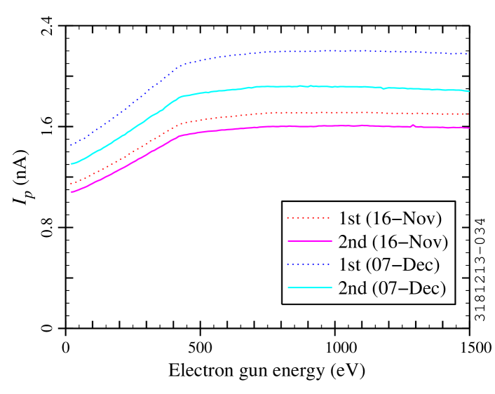
Figure 5: Repeated scans of $I_{p}$ as a function of gun energy (horizontal aC sample, 2010). The measurements were done before (dotted curve) and after (solid curve) an $I_{t}$ scan. Ideally, $I_{p}$ should be constant at 2 nA.

4 Measurement Method: Phase II Improvements

Our experience in Phase I led to iterations in the measurement method. Modifications for Phase II are described in this section, as outlined in Fig. 6; a time-line can be found in Appendix A. The measurement hardware and methods have been relatively stable since the start of Phase IIb in August 2012.

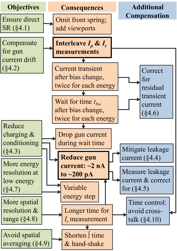
Figure 6: Flowchart showing the modifications to the SEY measurement method for Phase II and the interrelationships amongst various modifications. Changes with major ramifications are highlighted in bold type.

Our final procedure for SEY measurements in Phase IIb is as follows: (i) do a leakage scan (the purpose of which will be described in Section 4.5); (ii) warm up the electron guns for 30 to 60 minutes and then set $I_{p}\approx 200$ pA (Section 2.5); (iii) do an SEY scan; (iv) repeat the leakage scan. The leakage scan takes 40 minutes and the SEY scan takes 110 minutes. Including sample transfer, the full measurement takes about 5 hours. This requires us to measure the samples in parallel rather than sequentially, since the access time is typically 6 hours.

The final timing algorithm for SEY scans is significantly different from Phase I, as shown in Fig. 7. The focus and deflection are adjusted with energy (Fig. 7b-d); positive and negative bias are applied at each energy (Fig. 7f) for current measurements (Fig. 7g; a zoomed-in version is shown in Fig. 8) with the deflection rastered over multiple grid points (Fig. 7c-d). (For clarity, the time axis is not to scale and a simple 3 by 3 grid is shown.) Features of Fig. 7 will be discussed further in this section. Table 1 gives the final timing parameters.

Table 1: Timing parameters for Phase IIb SEY scans.

Symbol	Value	Description
$t_{m}$	$\sim 250$ ms	average and read out current
$t_{dw}$	50 ms	wait after setting gun deflection
$t_{cw}$	10 s	wait after setting gun current
$t_{bw}$	60 s	wait after setting bias

Figure 7: Timing schematic for SEY scans in Phase IIb: (a) gun energy, (b) focus, (c) horizontal and (d) vertical deflection, (e) gun emission current, (f) sample bias, and (g) sample current as a function of time for 2 iterations (75 eV, 100 eV) in the energy scan. In (g), the averaging of $I_{p}$ is in red and the averaging of $I_{t}$ is in green ($n_{x}$ and $n_{y}$ = number of horizontal and vertical grid points; $n=n_{x}n_{y}$). Gray lines: bias change (solid); increase in the gun current from the standby value to the full value (dashed); or deflection change (dotted).

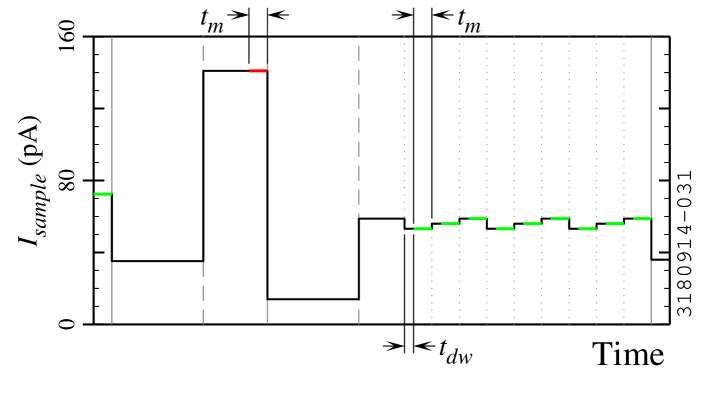
Figure 8: Zoomed-in timing schematic of sample current for SEY scans in Phase IIb, with the time intervals for averaging $I_{p}$ (red) and $I_{t}$ (green).

4.1 Ensuring Direct Photon Bombardment

The SR photons are nearly tangent to the beam pipe wall, so a sample recessed by $\geq 0.1$ mm does not receive any direct photons. As a result, in Phase I, we were unsure whether the samples were bombarded by direct photons; little difference was observed between the horizontal and 45^∘ samples. For Phase II, we took steps to ensure direct SR bombardment [36], and significant differences were observed in the early conditioning.

4.2 Mitigation of Electron Gun Current Drift

As discussed in Section 3, $I_{p}$ changes slowly with time. For the Phase I measurements on Al and aC-coated samples, the “before $I_{t}$” and “after $I_{t}$” measurements of $I_{p}$ differed by about 8% on average and by about 16% in the worst case. The first pair of measurements in Fig. 5 show typical reproducibility.

To reduce the systematic error due to $I_{p}$ drift, a new measurement procedure was developed for Phase II in which $I_{p}$ and $I_{t}$ measurements are interleaved. As shown in Fig. 7, the Phase II procedure is to set the gun energy, apply a positive bias to the sample, move the beam to the parking point and wait for the current to stabilize, measure $I_{p}$ at one grid point, apply a negative bias, park the beam and wait for the current to stabilize, measure $I_{t}$ for all desired grid points, and then proceed to the next energy. We wait for a time $t_{bw}=60$ s after a bias change (Table 1), a compromise between the need for a short measurement time and the need to allow the transient current to diminish (Section 4.6). The longer waiting time required us to reduce the number of energy steps (Section 4.7).

With the Phase II method, we estimate that the error in the current measurements due to gun current drift is $\mathrel{\hbox to0.0pt{\raise 2.15277pt\hbox{$<$}\hss}{\lower 2.15277pt\hbox{$\sim$}}}2$%.

4.3 Reduction of Charging and Parasitic Conditioning

Initial SEY measurements on samples with DLC coatings were done in 2011 in the off-line station. A Phase I measurement on DLC is shown in Fig. 9 (blue circles). The SEY curve appears distorted. We suspected that the distortion was due to charging of the surface by the electron beam, presumably owing to insulator-like properties of the DLC layer. Similar effects have been reported for other materials such as MgO [42].

To test the charging hypothesis, we remeasured the SEY with a long wait time ($\sim 3$ minutes) between energy steps to allow the surface to discharge, and with a smaller current ($I_{p}\sim 0.5$ nA instead of $\sim 2$ nA) to reduce the supply of charge to the sample. The beam was parked away from the measurement point while waiting. This resulted in a significant increase in SEY, as shown in Fig. 9 (red squares). The new curve is closer to what is measured for other materials, and is more consistent with other DLC measurements [43, 27, 30].

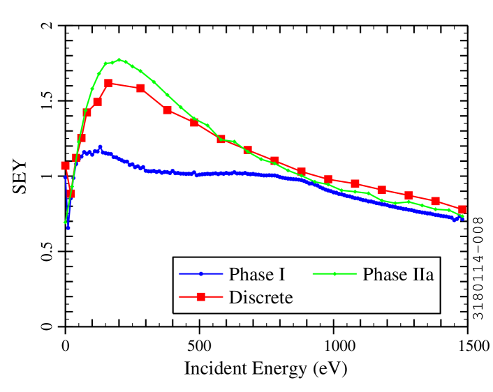
Figure 9: SEY as a function of incident electron energy for a DLC-coated Al sample (middle grid point, $\theta=25^{\circ}$). Blue: Phase I method ($I_{p}\sim 2$ nA, 5 seconds for each energy, 9 grid points). Red: “discrete” scan (large energy step, $I_{p}\sim 0.5$ nA, $\sim 3$ minutes waiting period with the beam parked away from the measurement point; 1 grid point). Green: Phase IIa method ($I_{p}<0.2$ nA, 9 grid points, beam parked away from measurement point).

The DLC results motivated us to reduce the gun current: in Phase II, we used $I_{p}\sim 0.2$ nA; a side benefit was to reduce parasitic conditioning, which, as discussed in Section 2.4, should be minimized. A complication is that, in Phase II, we switched the bias to measure $I_{p}$ and $I_{t}$ at each energy (Section 4.2), with an added settling time (Section 4.6). The longer wait increased the integrated current per energy step; to shorten the measurement time and reduce charging and conditioning, we adjusted the energy segmentation (Section 4.7). The net result was an increase in the integrated flux for the parking point and a decrease in integrated flux for other grid points. A measurement on the same DLC sample using the Phase IIa method is included in Fig. 9 (green diamonds). The differences between the discrete scan and the Phase IIa scan are mainly due to the leakage correction (Sections 4.5 and 5.2) included in the Phase IIa case.

In Phase IIb, an additional improvement was introduced: we decreased $I_{p}$ by a factor of $\sim 4$ while waiting for the sample current to stabilize after a bias change. We return to the nominal gun parameters for a time $t_{cw}=10$ s to allow the gun current to stabilize before the measurement (Fig. 7). The gun current modulation reduces the dose to the parking point by a factor of $\sim 3.5$. Though different in the details, our modulation method is conceptually similar to previously-used techniques for insulating materials (see [42], for example).

With Phase IIb parameters, one SEY scan produces an integrated electron flux of $\sim 0.8$ $\mu$C/mm² for the parking point and $\mathrel{\hbox to0.0pt{\raise 2.15277pt\hbox{$<$}\hss}{\lower 2.15277pt\hbox{$\sim$}}}12$ nC/mm² for the other grid points. In past studies on electron gun conditioning by other groups, the peak SEY decreased by $\mathrel{\hbox to0.0pt{\raise 2.15277pt\hbox{$<$}\hss}{\lower 2.15277pt\hbox{$\sim$}}}10$% for doses of order 1 $\mu$C/mm² for Cu [24, 28], TiN [40], and Al [44]. Based on this, we would expect to see some conditioning at the parking point. However, there may be less conditioning in our Phase II SEY scans because the electron energy is low for much of the scan, and it has been found that conditioning is less efficient at low energies [45].

We did not see a significant difference in the parking point’s SEY for Cu, stainless steel, TiN, or Al in Phase II. As noted above, DLC is more susceptible to charging. Off-line measurements on an unconditioned DLC sample with Phase IIb parameters showed a decrease in the measured SEY at the parking point with current modulation ($\sim 7$%) and a larger decrease without current modulation ($\sim 24$%). On the other hand, a conditioned and air-exposed DLC sample did not show a difference in measured SEY at the parking point. Additional measurements are being done in the off-line station to better quantify the susceptibility to charging and conditioning and check the reproducibility of our observations.

4.4 Leakage Current: Mitigation

Ideally, the picoammeter measures only the current due to primary and secondary electrons. In reality, because the insulators are imperfect, additional current (“leakage current”) flows through the picoammeter to ground when the sample is biased. The leakage current should be a small fraction of $I_{p}$ to avoid systematic errors in the calculated SEY [32]. In Phase I ($I_{p}\sim 2$ nA), no leakage corrections were applied. Because the relative contribution from the leakage current increases as the gun current decreases, the leakage current was investigated while preparing for Phase II measurements with $I_{p}\sim 0.2$ nA.

Measurements indicated that the leakage current was strongly correlated with the ambient humidity. At high humidity, we found that the leakage could be as high as several nA (hence exceeding $I_{p}$) and could vary significantly in the time needed for an SEY scan, which could produce large systematic errors.

We took steps to minimize the leakage paths in the measurement circuit [36]. After these modifications, the main leakage paths were found to be the insulating stand-offs and the ceramic break (shown in green in Fig. 4b).

The decrease in resistivity of insulators due to moisture has been documented in the literature in the past century (see, e.g., [46, 47, 48]). In a humid environment, current is conducted along insulator surfaces, where there is a layer of moisture from the ambient air. These considerations led us to a redesign: (i) the original G10 stand-offs were replaced by similar parts with a smoother surface finish, more careful cleaning, and blind holes in lieu of through holes; (ii) a nitrogen gas “blanket” was made to isolate the ceramic break from the air. A Teflon tube (shown in blue in Fig. 4b) was attached to the grounded side of the ceramic break, with a small gap on the biased side to avoid adding another leakage path (the blanket region is shown in orange in Fig. 4b). We used a steady flow of N₂ gas (about 2.5 SCFH $\approx$ 20 mL/s per station) to establish the blanket. The gas source is boil-off from the building’s liquid N₂ storage Dewar.

At high humidity, the nitrogen blanket alone did not produce a low and stable leakage current; we had to first warm the ceramic with a heat gun to remove the existing moisture. At low humidity, the leakage currents with and without gas flow were comparable. See Appendix C for more information.

After the modifications to the system, the leakage current was $\mathrel{\hbox to0.0pt{\raise 2.15277pt\hbox{$<$}\hss}{\lower 2.15277pt\hbox{$\sim$}}}30$ pA at $V_{b}=150$ V. This corresponds to an error of $\mathrel{\hbox to0.0pt{\raise 2.15277pt\hbox{$<$}\hss}{\lower 2.15277pt\hbox{$\sim$}}}14$% in the $I_{p}$ measurement for Phase II parameters (not including the transient contribution, which is discussed in Section 4.6). Repeated measurements indicated that the leakage current still varies over time, even with the gas blanket. The variation can be as much as a factor of 2 over long periods; see Appendix D for more information.

4.5 Leakage Current: Measurement

Since the leakage current is not negligible relative to $I_{p}$ and varies over time even with mitigation, we measure the leakage current prior to each SEY scan. The leakage scan is done with the same procedure as the SEY scan, but with the gun turned off. We repeat several iterations of positive and negative sample bias to allow the current to stabilize; however, we perform fewer iterations for the leakage scan (16) than for the SEY scan (44). The measured values of $I_{p}$ and $I_{t}$ are corrected by subtracting the measured leakage current for the corresponding bias before calculating SEY (Section 5.2).

Time permitting, a second leakage scan is done after the SEY scan to quantify the leakage current stability. Typically, the leakage currents before and after the SEY scan agree within $\pm 2$ pA for $V_{b}=+150$ V and within $\pm 0.5$ pA for $V_{b}=-20$ V. Hence we estimate that the leakage current drift contributes an error in the corrected currents of $\sim 1$% of $I_{p}$.

4.6 Transient Current: Mitigation

A bias change produces a transient in the sample current due to the stray capacitance of the system and the response of the picoammeter. The stray capacitance includes a contribution from the triaxial cable and the SEY station, whose biased positioner arm is in proximity to the grounded surroundings (Fig. 4b).

The transient current peaks at about 0.5 nA (hence exceeding $I_{p}$ for Phase II) with a decay time of order 30 s (examples are included in Appendix B). Ideally, one would wait for the current to reach its equilibrium value before starting the measurement. This could be done in Phase I, since the bias voltage was switched infrequently (twice per SEY scan).

On the other hand, with the Phase II procedure to mitigate the gun current drift, the bias is switched twice for each energy (Fig. 7f), making a long wait time after each bias change impractical. Hence a compromise solution was necessary: waiting for time $t_{bw}=60$ s after a bias change, reducing the number of energy steps (Section 4.7), and correcting for the residual effects from the transients. Because the leakage scans described above are done while switching the bias with the same timing algorithm as is used for the SEY scans, the correction for the leakage current also corrects for the residual transient current, which is about 4% of $I_{p}$ for the Phase II parameters.

The transient response produces a change in the leakage current over the time required to measure all of the grid points in the double scan (see Fig. 11 below). We record the time stamp along with the current, as the time elapsed since a bias change varies due to skipping of grid points (Section 4.8) and compensation of the waiting time (Section 4.10). A time dependence is included in the leakage correction to account for the change in current during the $I_{t}$ measurements (Section 5.2).

4.7 Energy Resolution and Segmentation

Phase I measurements were done with a fixed energy step of 10 eV. Because low-energy electrons are important to the build-up of the electron cloud, a smaller step was of interest for low energies. In Phase II, both $I_{p}$ and $I_{t}$ were measured in a single energy scan (Section 4.2), with longer waiting times at each energy (Section 4.6). To keep the overall measurement time within the schedule constraints, the energy step was increased for high energies (further motivated by the need to minimize charging and parasitic conditioning, as discussed in Section 4.3). The final Phase II method was to segment the energy range into 5 pieces, with an initial step of 1 eV, a final step of 75 eV, and a total of 44 energies [36].

4.8 Improved Spatial Resolution and Range

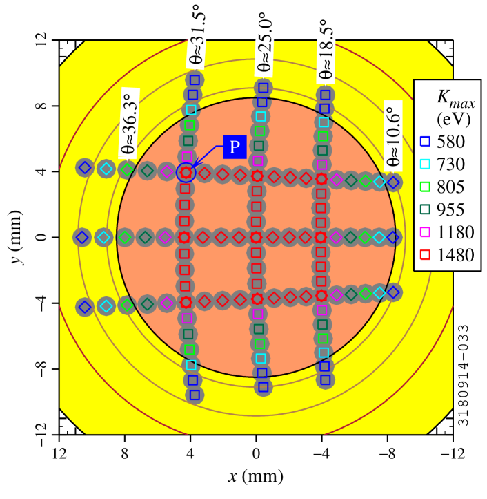
Figure 10: Grid points for double scans ($x$ and $y$ are the horizontal and vertical distance from the middle of the sample, respectively). Legend: maximum incident energy measured for each grid point. Squares: first array; diamonds: second array. Solid gray circles: estimated beam spot size at high gun energy. The approximate incident angle ($\theta$) is indicated for selected grid points. Orange: sample face; yellow: sample shoulder. P: parking point.

As discussed above, the Phase I measurements were done over a 3 by 3 grid. We implemented scans with increased range and resolution in Phase II to get a better picture of the SEY’s dependence on position and angle. A uniformly-spaced grid with high resolution and full range is not practical for weekly measurements, so we scan over 3 horizontal segments and 3 vertical segments only. (Occasionally, scans with high resolution and full range are done when additional time is available.) The grid points are shown in Fig. 10. One complication is that the largest deflections cannot be reached at high energies, because the gun’s deflecting electrodes are limited to $\pm 150$ V. The colors in Fig. 10 indicate the maximum energy measured for each grid point. The DAQP skips out-of-range points, which complicates the timing, as will be discussed in Section 4.10.

For simplicity, the grid point layout shown in Fig. 10 is measured using two arrays of gun deflections. As a result, 9 of the grid points are measured twice (the repeated points coincide with the 3 by 3 grid of Phase I). This provides additional information about systematic and statistical errors.

For simplicity, the gun deflection is varied linearly between grid points, leading to a constant increment in the tangent of the deflection angle. Because the gun axis is 25^∘ from the sample axis, the grid point spacing is not exactly left-right symmetric. Moreover, the sample face is curved, which shifts the grid points slightly near the upper and lower edges of the sample. These asymmetries in the grid layout can be seen in Fig. 10.

In Fig. 10, the gray circles indicate the estimated beam size at 1500 eV (not accounting for possible distortion in the beam spot for large deflecting angles). There is overlap between adjacent points over most of the sample. The estimated beam spot size is smaller at intermediate energies (Section 2.5); for the smaller spot size, none of the grid points overlap.

4.9 Spatial Resolution: Time Control and Hand-Shaking

In Phase I, we unintentionally used incompatible timing parameters for the picoammeter and the DAQP, such that $I_{t}$ measurements were averaged over multiple grid points. In Phase II, we decreased the averaging time and implemented a “hand-shaking” algorithm: after setting the gun parameters, the DAQP waits for the settling time $t_{dw}$, and then instructs the picoammeter to clear its buffer, average the current, and return the averaged value. The DAQP waits for the picoammeter’s value before proceeding, which avoids unintentional averaging. With the final Phase II method, the current is averaged over $\frac{1}{6}$ sec, and the net measurement time per grid point is about 0.3 sec.

4.10 Time Control: Cross-Talk Avoidance

As discussed in Section 2.6, shielded cables connect the sample positioner arms to the picoammeters, but the positioner arms are not electrically shielded. The stations are relatively close together ($\sim 0.4$ m apart at the beam pipe). As shown in Fig. 7f, the Phase II SEY scan algorithm requires two steps in the bias voltage for each energy. We observed that a bias change on one sample produces a spike in the measured current of the other sample. With Phase II parameters, the current perturbation can be up to $\sim 50$% of $I_{p}$. If the bias of one sample is changed while the current of the other sample is being measured, this can produce a noise spike in the measured SEY.

To avoid noise spikes, we implemented a delay between the scan start times. In Phase IIb, the bias wait time is 60 s and the $I_{t}$ measurements take $\sim 35$ s, allowing for a timing margin of $\sim 12$ s with a start delay of 47 s between systems.

Even with start time control, spikes still occurred occasionally. Further investigation indicated that the time to measure one grid point is sometimes much longer ($\sim 1$ s) than nominal (0.3 s). When the longer delays are random, there is little cumulative effect. With the large number of Phase II grid points, a cluster of longer delays sometimes occurs for one system, accumulating enough time difference to produce cross-talk again.

To eliminate the cross-talk problem reliably, we modified the timing algorithm. The DAQP uses the wait times and expected measurement time per point to predict the overall time per energy step. After each energy step, the DAQP checks the time elapsed. In the next energy step, it adjusts the wait time to compensate for the actual time of the previous step being different from the desired time. This prevents timing variations from accumulating a large time offset. It has the side effect that the wait time varies from one energy to another; this is taken into account in the data analysis, as discussed in Section 5.2.

A complication is that the number of grid points decreases for $K>580$ eV (Section 4.8). Hence the DAQP must account for skipped points when calculating the expected time. As long as their start times have the appropriate offset, the 2 systems remain synchronized as the time per iteration decreases.

5 Data Analysis

The SEY is calculated from $I_{p}$ and $I_{t}$ using Eq. 2. The gun energy is corrected to account for the electrostatic deflection and the sample bias. The measured currents are corrected to account for the leakage and transient current.

5.1 Momentum Corrections

Paired electrodes at the exit of the gun deflect the electrons by the desired horizontal and vertical angles ($\alpha_{x}$, $\alpha_{y}$). Because the kicks are electrostatic, they also change the electrons’ kinetic energy. In the non-relativistic case, the kinetic energy $K_{g}$ of the electrons is related to the set point value $K_{gsp}$ via

$$K_{g}=K_{gsp}[1+\tan^{2}(\alpha_{x})+\tan^{2}(\alpha_{y})]\;.$$ (3)

For Phase IIb parameters, the energy correction is $\leq 9.5$%.

The SEY is a function of the kinetic energy $K$ and angle $\theta$ of the incident primary electron. Because the sample is biased, $K$ is shifted from the gun energy ($K_{g}$) by the bias voltage ($V_{b}$):

$$K=K_{g}+q_{e}V_{b}\;,$$ (4)

where $q_{e}$ is the electron charge magnitude. Hence the incident energy is smaller than $K_{g}$ by 20 eV when we measure $I_{t}$ and larger by 150 eV when we measure $I_{p}$. Ideally, the negative bias repels all of the secondary electrons from the sample, while the positive bias prevents the escape of any secondaries. In the ideal case, assuming that the intrinsic $I_{p}$ is independent of $V_{b}$, we may use $V_{b}=-20$ V in Eq. 4 to calculate the appropriate incident energy $K$ associated with the measured SEY.

Because the primary electrons’ incident angle is not normal to the sample ($\theta\neq 0$), the sample bias can also shift the incident angle and impact position. At present, our data analysis does not account for these effects. As a result, the reader should be cautious about making inferences about the SEY for $K\mathrel{\hbox to0.0pt{\raise 2.15277pt\hbox{$<$}\hss}{\lower 2.15277pt\hbox{$\sim$}}}100$ eV based on our measurements [36].

5.2 Correction for Leakage and Transient Current

In Phase II, we mitigated (Section 4.4) and measured (Section 4.5) the leakage current, including the transient contribution (Section 4.6). To properly correct the SEY, we developed a model for the leakage current that includes the transient contribution, as described in Appendix B.

Figure 11: Example of measurements of leakage current as a function of time while switching the bias voltage (stainless steel samples, Aug 2012). (a) Leakage measurements with $V_{b}=+150$ V for $I_{p}$ correction (1 point per iteration); (b) leakage measurements with $V_{b}=-20$ V for $I_{t}$ correction (120 points per iteration); (c) same as (b), with zoomed-in view of the penultimate iteration. Light colors (magenta, cyan): uncorrected. Dark colors (red, blue): corrected; the corrected values should be zero.

Fig. 11 shows examples of leakage scans. The light markers indicate the measured (“raw”) current. With $V_{b}=150$ V (Fig. 11a), the leakage current is 20 to 30 pA. With $V_{b}=-20$ V (Fig. 11b), the leakage current is smaller in magnitude and opposite in sign. The measurements with negative bias are repeated 120 times, following the same timing algorithm as for the SEY scans; the current changes by 2 to 3 pA in this time, which is about 2% of $I_{p}$ for Phase II parameters.

The dark markers in Fig. 11 show the result of applying the time-dependent leakage correction. Over most of the scan, the corrected current is $\pm 1$ pA or less, which is about 1% of $I_{p}$. There are larger discrepancies during the first few minutes of the scan, illustrating the usefulness of the iterations.

As can be seen in Fig. 11b, the time-dependent correction compensates for the transient behavior reasonably well. Zooming in on one iteration (Fig. 11c), we see that the corrected current differs from zero, but the systematic differences are comparable to the noise in the measurement. The time-dependent correction uses the recorded time stamp for each current measurement, so that variations in the time per grid point and timing adjustments to avoid cross-talk (Section 4.10) are accounted for.

Because $I_{p}$ and $I_{t}$ are both corrected, the effect on SEY can partially cancel. For example, if the uncorrected and corrected $I_{t}$ values are small relative to $I_{p}$, SEY $\approx 1$ and the corrections to $I_{p}$ produce little change in SEY. Fig. 12 shows examples of the current correction’s impact on SEY. For unconditioned Al with a peak SEY of $\sim 2.5$, the correction increases the peak by $\sim 10$%. For reconditioned TiN with a peak SEY of $\sim 1$, the correction decreases the peak by $\sim 5$%.

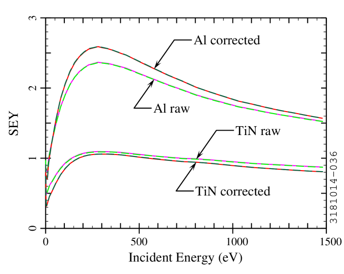
Figure 12: Measurements of SEY as a function of energy without correction (light colors) and with correction for leakage current and transient response (dark colors). (Middle grid point of 45^∘ sample, $\theta=25^{\circ}$.) Upper curves: unconditioned Al (Jan 2013). Lower curves: reconditioned TiN (Nov 2012). Solid curves: first measurement. Dashed curves: repeat measurement.

In Fig. 12, both the first (solid curves) and the repeated (dashed curves) measurements are shown, since this grid point is measured twice in the double scan; the first and second $I_{t}$ measurements are separated in time by $\sim 17$ s. The $I_{t}$ values are corrected by different amounts to account for the current transient. However, there is little difference in SEY, which indicates that the variation in $I_{t}$ over the time required to scan the grid points has little impact on SEY.

Thus, in the examples above, the magnitude of the leakage current is $\mathrel{\hbox to0.0pt{\raise 2.15277pt\hbox{$<$}\hss}{\lower 2.15277pt\hbox{$\sim$}}}15$% of $I_{p}$, which is typical for measurements with leakage mitigation; the unmitigated leakage current could be $\mathrel{\hbox to0.0pt{\raise 2.15277pt\hbox{$>$}\hss}{\lower 2.15277pt\hbox{$\sim$}}}100$% of $I_{p}$ under adverse conditions. The correction in the SEY due to the leakage current is $\mathrel{\hbox to0.0pt{\raise 2.15277pt\hbox{$<$}\hss}{\lower 2.15277pt\hbox{$\sim$}}}10$%, which is also typical for Phase II measurements. With 120 grid points, there is a clear time dependence in the leakage current due to the bias switch transient. The time-dependent leakage correction accounts for this effectively, but the impact on the SEY is small for Phase II, as we used a 60 s wait time after a bias switch. Hence it may be possible to use a shorter wait time in future measurements.

5.3 Uncertainties

As discussed above, most Phase II modifications were oriented toward reducing systematic errors. Table 2 summarizes the estimated error contributions from various sources for various scenarios. The values apply to both $I_{p}$ and $I_{t}$, but are expressed as a percentage of $I_{p}$ (it is not straightforward to estimate the error as a fraction of $I_{t}$).

Table 2: Summary of estimated current measurement errors as a percentage of $I_{p}$. For errors due to leakage and transient currents, the Phase II value of $I_{p}\sim 200$ pA is assumed. The scenarios used for the final Phase II procedure are in bold type. HH = high humidity, LH = low humidity (as quantified in Appendix C), SC = static correction, TDC = time-dependent correction.

Source	Mitigate	Correct for	Error
Gun current	no (Ph. I)	no	$\mathrel{\hbox to0.0pt{\raise 2.15277pt\hbox{$<$}\hss}{\lower 2.15277pt\hbox{$\sim$}}}16$%
drift (§4.2)	yes (Ph. II)	no	$\mathrel{\hbox to0.0pt{\raise 2.15277pt\hbox{$<$}\hss}{\lower 2.15277pt\hbox{$\sim$}}}2\%$
Leakage	no (HH)	no	$\mathrel{\hbox to0.0pt{\raise 2.15277pt\hbox{$>$}\hss}{\lower 2.15277pt\hbox{$\sim$}}}100$%
current	no (LH)	no	$\mathrel{\hbox to0.0pt{\raise 2.15277pt\hbox{$<$}\hss}{\lower 2.15277pt\hbox{$\sim$}}}14$%
(§4.4–4.5)	no (HH)	yes	$\mathrel{\hbox to0.0pt{\raise 2.15277pt\hbox{$>$}\hss}{\lower 2.15277pt\hbox{$\sim$}}}100$%
	no (LH)	yes	$\mathrel{\hbox to0.0pt{\raise 2.15277pt\hbox{$<$}\hss}{\lower 2.15277pt\hbox{$\sim$}}}1$%
	yes	no	$\mathrel{\hbox to0.0pt{\raise 2.15277pt\hbox{$<$}\hss}{\lower 2.15277pt\hbox{$\sim$}}}14$%
	yes	yes	$\mathrel{\hbox to0.0pt{\raise 2.15277pt\hbox{$<$}\hss}{\lower 2.15277pt\hbox{$\sim$}}}1\%$
Transient	no ($t_{bw}=0$)	no	$\mathrel{\hbox to0.0pt{\raise 2.15277pt\hbox{$>$}\hss}{\lower 2.15277pt\hbox{$\sim$}}}100$%
current	yes ($t_{bw}=60$ s)	no	$\mathrel{\hbox to0.0pt{\raise 2.15277pt\hbox{$<$}\hss}{\lower 2.15277pt\hbox{$\sim$}}}4$%
(§4.6, §5.2)	yes ($t_{bw}=60$ s)	yes (SC)	$\mathrel{\hbox to0.0pt{\raise 2.15277pt\hbox{$<$}\hss}{\lower 2.15277pt\hbox{$\sim$}}}2$%
	yes ($t_{bw}=60$ s)	yes (TDC)	$\mathrel{\hbox to0.0pt{\raise 2.15277pt\hbox{$<$}\hss}{\lower 2.15277pt\hbox{$\sim$}}}1\%$
Cross-talk	no (Ph. IIa)	no	$\mathrel{\hbox to0.0pt{\raise 2.15277pt\hbox{$<$}\hss}{\lower 2.15277pt\hbox{$\sim$}}}50$%
(§4.10)	yes (Ph. IIb)	no	none

Using Eq. 2, one can infer the impact of errors in the measurement of $I_{p}$ and $I_{t}$ on the calculated SEY. For Phase IIb, we expect the items listed in Table 2 to produce a systematic error in SEY of at most a few percent for $0\leq$ SEY $\leq 2$.

Errors due to charging and conditioning are not included in Table 2. From Fig. 9, we infer that the error in SEY due to charging was $\sim 45$% for DLC with the Phase I method. With the Phase IIb method, as discussed in Section 4.3, we observe some charging or conditioning of unconditioned and susceptible materials at the parking point, which decreases the measured SEY by $\mathrel{\hbox to0.0pt{\raise 2.15277pt\hbox{$<$}\hss}{\lower 2.15277pt\hbox{$\sim$}}}7$% with mitigation (see also Section 6.3).

Overall, we expect the items considered in Section 4 to contribute a few percent to the systematic error in the SEY for most grid points (and $\mathrel{\hbox to0.0pt{\raise 2.15277pt\hbox{$<$}\hss}{\lower 2.15277pt\hbox{$\sim$}}}10$% for the parking point) with the Phase IIb method. We estimate that the statistical errors are of the same order. A future paper will include more detailed results with a more complete error analysis.

6 Examples of SEY Results

Some examples of SEY measurements are presented in this section. The beam dose is given in terms of the integrated current of stored $e^{-}$ bunches; 1 amp$\cdot$hour corresponds to about $3\cdot 10^{21}$ photons/m of direct SR at the location of the samples.

6.1 SEY as a Function of Energy

Fig. 13 shows the measured SEY of the $45^{\circ}$ DLC-coated sample as a function of energy for different beam doses. The peak in the SEY is at about 200 eV. There is a clear decrease in SEY with beam dose: before conditioning, the peak SEY is about 1.8; for doses $>20$ A$\cdot$h, the peak SEY is in the range of 1.1 to 1.2. The changes due to conditioning are large compared to the estimated errors in the measurement.

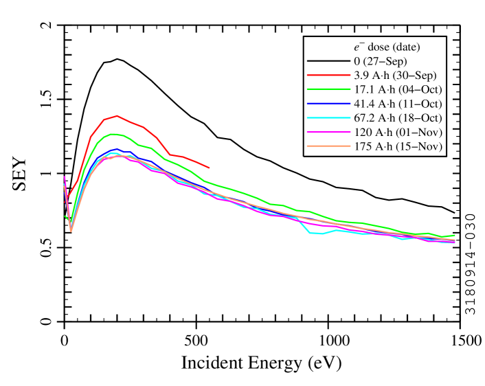
Figure 13: SEY as a function of incident energy for the 45^∘ DLC sample (middle grid point, $\theta=25^{\circ}$, Phase IIa, Sep-Nov 2011).

6.2 Peak SEY as a Function of Vertical Position

Fig. 14 shows measurements of the peak SEY as a function of vertical position for stainless steel. The gun deflection is converted to azimuthal angle along the beam pipe, with one sample (horizontal) centered at 0 and the other at $-45^{\circ}$.

Figure 14: Peak SEY of stainless steel samples (Phase IIb, Aug-Sep 2012) as a function of position expressed in terms of the azimuthal angle along the beam pipe (BP). (a) Scans along the middle of the sample ($\theta\approx 25^{\circ}$) for different beam doses; (b) scans at different incident angles for the 0.05 A$\cdot$h case, with repeated points included. The vertical lines indicate the edges of the sample (black dotted: $\theta\approx 25^{\circ}$; solid gray: $\theta\approx 18.5^{\circ},31.5^{\circ}$).

Fig. 14a compares different beam doses. Before beam exposure (black), the peak SEY is about 1.8 and is approximately constant. After a small beam dose (red), a dip in the SEY appears near the middle of the horizontal sample, presumably due to direct SR. For high doses, the SEY decreases and returns to being approximately independent of position. The observed differences are again large compared to the estimated errors.

Fig. 14b compares the peak SEY as a function of vertical position for 3 different horizontal deflections (Fig. 10, square markers) for the 0.05 A$\cdot$h case (the red case in Fig. 14a). The legend indicates the approximate angle of incidence ($\theta$). The dip in peak SEY at $\sim 2^{\circ}$ is seen in all 3 scans.

6.3 Reproducibility

Nine grid points are measured twice (as seen in Fig. 10), which provides a check of the short-term reproducibility of the measurements. In Fig. 14b, vertical scans (Fig. 10, squares) are shown in red; repeated points from horizontal scans (Fig. 10, diamonds) are shown in blue. The repeated values are reasonably consistent. This indicates that the features seen in the vertical scans are reproducible and that the system is able to properly resolve the dependence of SEY on position.

We can repeat measurements occasionally during extended access periods. Repeated measurements on Al samples (1 or 2 days apart, without intervening exposure to beam) in Phase II indicate that the measured SEY can vary by up to 5% or more for a few grid points. For most of the 120 grid points, the SEY varies by a few percent or less, consistent with what we expect based on the systematic uncertainties (Section 5.3). Thus the measured changes from scrubbing are large compared to the day-to-day reproducibility of the measurements.

7 Conclusion

We have developed an in-situ secondary electron yield measurement system to observe conditioning of metal and coated samples by CESR beams. We have made iterative improvements in the measurement method to reduce charging and conditioning by the electron gun; mitigate and correct for the leakage current and transient current; eliminate cross-talk between the adjacent SEY stations; and mitigate gun current drift. We have reduced the systematic error due to these effects to a few percent, allowing us to measure the dependence of the SEY on beam dose, position, and angle with better resolution.

There is room for additional improvement in the techniques. Sources of systematic error that we have not yet accounted for include (i) the escape of elastic and rediffused secondaries during the measurement of the primary current, and (ii) the deflection of low-energy primary electrons by the sample bias. A more direct measurement method may help further reduce the systematic errors. Measuring the energy distribution of the secondary electrons would allow us to distinguish between elastic, rediffused, and true secondaries. Additional improvements to the apparatus and techniques might allow us to reduce the measurement time and decrease the incidence of noise spikes in the current due to nearby activity. Some of the improvements described above may not be practical for our in-situ apparatus, and may require an out-of-tunnel SEY measurement system.

Our ultimate goal is to use the SEY measurements under realistic conditions to constrain the SEY model parameters as much as possible; this will help improve the predictive ability of models for electron cloud build-up, allowing for more successful electron cloud mitigation in future accelerators, so that they can achieve better performance and higher reliability.

Appendix A Measurements and Modifications Time-Line

Table A.1 outlines the time-line for SEY measurements and system modifications in Phase I and Phase II.

Table A.1: SEY in-situ measurements and improvements in techniques. GCD = gun current drift; resol. = resolution; R & R = resolution and range.

Samples	Dates	Comments
Phase I Measurements
TiN	Jan-Aug 2010	Commission systems
Al 6061	Aug-Nov 2010	Remove vacuum gauges
aC	Nov 2010-
	Jan 2011
Phase IIa Development
(none)	Jan-Aug 2011	Ensure direct SR (§4.1); mi-
		tigate GCD (§4.2), charging
		(§4.3), & leakage (§4.4–4.6)
Phase IIa Measurements
DLC	Sep-Nov 2011	Investigate spatial resol.
TiN	Nov 2011-	Improve spatial resol. (§4.9);
2nd pair	Mar 2012	variable energy step (§4.7);
		investigate spatial R & R
Cu	Mar-Jul 2012	Improve spatial R & R
Phase IIb Measurements
Stainless	Aug-Sep 2012	Full spatial R & R (§4.8); mi-
steel		tigate parasitic conditioning
316		(§4.3) & cross-talk (§4.10)
TiN	Oct 2012-	Recondition after air
2nd pair	Jan 2013	exposure
Al 6063	Jan 2013-	Long-term conditioning

Appendix B Model for Leakage and Transient Current

The leakage current changes slowly in the time required to measure $I_{t}$ for all of the grid points (Section 5.2). This led us to develop a model to account for both the leakage current and the transient current. Additional details are provided in [36].

We measured the sample current $I$ as a function of time $t$ after stepping the bias voltage. For a circuit with resistive and capacitive elements, the current should decay exponentially towards a steady-state value $I_{\infty}$ after a bias step. This was not a good description of the current we measured. Our inference is that the picoammeter is an active element of the circuit.

After a step from $V_{b}=V_{0}$ to $V_{b}=V_{2}$ at time $t_{1}$, we found

$$I(t)\approx\Gamma_{\parallel}\left(\frac{V_{2}-V_{0}}{t-t_{1}}\right)+\frac{V_{2}}{R_{\parallel}}\;,$$ (B.1)

where $\Gamma_{\parallel}$ and $R_{\parallel}$ are constants. For $t\rightarrow\infty$, $I(t)\rightarrow I_{\infty}=V_{2}/R_{\parallel}$, consistent with a simple circuit with resistance $R_{\parallel}$ from sample to ground. The constant $\Gamma_{\parallel}$ has dimensions of capacitance, and can be thought of as being a “capacitance-like” quantity. Since Eq. B.1 is not derived from a circuit, we refer to it as a “semi-empirical” model.

Figure B.1: Measured current as a function of time for the 45^∘ SEY station with a step in the sample bias between $-20$ V and $+150$ V at time $t_{1}$, with (a) linear-log, and (b) log-log scale. The solid cyan curve represents the model, using best match parameters of $\Gamma_{\parallel}=2.3$ pF and $R_{\parallel}=10$ T$\Omega$.

Fig. B.1 shows measurements on the 45^∘ system. The time at which the bias is stepped ($t_{1}$) is subtracted from $t$ and the steady-state current ($I_{\infty}$) is subtracted from $I(t)$. Additionally, $I-I_{\infty}$ is multiplied by a sign correction coefficient $s=\pm 1$ to compare upward and downward steps in $V_{b}$ on the same footing.

It is clear from the log-linear scale of Fig. B.1a that the current does not decrease exponentially to its steady-state value. The transient current is as high as about $\pm 500$ pA, which is much larger than the steady-state current of $\pm 15$ pA or less.

Fig. B.1b shows the current as a function of time on a log-log scale. The cyan curves represent the semi-empirical model, which fits the measurements reasonably well when $t-t_{1}>30$ s. For $t-t_{1}<30$ s, the model differs significantly from the measured current. However, the relevant time interval for SEY measurements starts 60 s after the bias step and lasts for 35 s (indicated by the dotted lines). Hence the discrepancies for $t-t_{1}<30$ s are not a problem for our Phase II procedure.

The parameter values to fit the measured current are in the range of $\Gamma_{\parallel}=0.5$ to $3$ pF and $R_{\parallel}=6$ to $25$ T$\Omega$; per Appendix D, the best-fit values are different for each SEY station and vary with time, leading us to do a leakage scan prior to each SEY scan (Section 4.5). We use the parameter values from the leakage scan to correct the currents for the subsequent SEY scan, as described in more detail in [36].

Appendix C Unmitigated Leakage Current

In Phase IIb, some measurements without leakage mitigation were done to better understand the final systems’ behavior. We measured the leakage on the off-line station at various humidities (set by the outside air conditions as modified by the climate control system) with the N₂ gas flow off; we measured the relative humidity (RH) using a portable hygrometer.

Fig. C.1 shows the leakage current ($I_{leak}$) as a function of humidity for $V_{b}=150$ V and $-20$ V. For RH $\mathrel{\hbox to0.0pt{\raise 2.15277pt\hbox{$>$}\hss}{\lower 2.15277pt\hbox{$\sim$}}}30$%, the leakage increases rapidly, changing by more than a factor of 10 between the lowest and highest humidities. For RH $\mathrel{\hbox to0.0pt{\raise 2.15277pt\hbox{$<$}\hss}{\lower 2.15277pt\hbox{$\sim$}}}30$%, the leakage is low, though it still shows some variation.

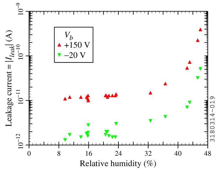
Figure C.1: Measured leakage current as a function of humidity for the off-line station without mitigation (temperature = 21.5 to 23.5^∘C).

We can infer the resistance to ground ($R_{leak}$) from the bias and the leakage current. The calculated values of $R_{leak}$ for positive and negative bias are roughly consistent; per Appendix B, ideally we should have $R_{leak}=R_{\parallel}$. At low humidity, $R_{leak}$ is in the range of 10 to 20 T$\Omega$, consistent with the values of $R_{\parallel}$ with mitigation of Appendix D.

For RH $\mathrel{\hbox to0.0pt{\raise 2.15277pt\hbox{$>$}\hss}{\lower 2.15277pt\hbox{$\sim$}}}35$%, Fig. C.1 shows that a small change in humidity produces a large change in leakage. Hence SEY measurements in a humid environment without a gas blanket are likely to have large errors due to small humidity variations. Fig. C.2 shows leakage scans without gas flow at different humidities. With low humidity (light blue), RH decreased from 15.9% to 15.5% during the scan. The leakage remained low and stable. With high humidity (dark blue), RH varied from 43.1% up to 46.0% and then down to 42.5%. Correspondingly, the leakage varied by a factor of $\sim 4$. Measurements at $V_{b}=-20$ V (not shown) were interleaved with the measurements at $+150$ V, with similar trends. Thus, as anticipated, a humid environment gives poor leakage current stability.

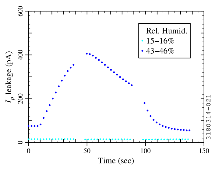
Figure C.2: Leakage scans for the off-line station without mitigation at different ambient humidities ($V_{b}=+150$ V, temperature = 21.5 to 23.5^∘C).

We conclude that, in a dry environment (RH $\mathrel{\hbox to0.0pt{\raise 2.15277pt\hbox{$<$}\hss}{\lower 2.15277pt\hbox{$\sim$}}}30$%), the leakage current for our SEY stations is relatively stable, and mitigation is not needed. With higher humidity and no mitigation, leakage corrections are large: at RH = 46%, the leakage with $V_{b}=+150$ V exceeds our Phase II value of $I_{p}\approx 200$ pA, and varies significantly over the time of an SEY scan. A dry nitrogen blanket ensures low and stable leakage current. However, a dry environment does not remove the need to measure the leakage current; even with the N₂ blanket, we observe long-term variation in the leakage, as discussed in the next section.

Appendix D Mitigated Leakage Current

Figure D.1: Comparison of long-term trends: (a) measured leakage currents, (b) tunnel air temperature, (c, d) leakage model parameters as a function of time. The measurements were done over approximately 2.5 years, from 27 Sep 2011 (time = 0) to 25 Feb 2014 (time = 882 days). The gray lines correspond to quarterly calendar dates. Temperatures were measured with thermocouples in the tunnel at 40E ($\sim 10$ m East of the SEY stations) and 40W ($\sim 10$ m to the West of the stations).

In Phase II, we used an N₂ gas blanket to mitigate leakage (Section 4.4) and did a leakage scan prior to each SEY scan (Section 4.5). Measured leakage currents are shown in Fig. D.1a: $I_{pl}$ and $I_{tl}$ were measured with $V_{b}=+150$ V and $-20$ V, respectively. As can be seen, the leakage current has varied by a factor of $\sim 2$ in Phase II. The leakage current changes enough over time to make repeated leakage scans necessary—a constant-leakage assumption would introduce significant systematic errors into the SEY calculation.

The leakage current varies non-randomly, though it does not decrease steadily or change seasonally. Fig. D.1a suggests that the leakage current is higher when the accelerator is running and lower during summer and winter down periods. One difference between high-current operation and down periods is the tunnel air temperature, as illustrated in Fig. D.1b. The air temperature increases by about 8^∘C when CHESS currents are stored. Comparison of Figs. D.1a and D.1b shows that the leakage current is indeed correlated with temperature. This correlation could come about if the leakage properties of the ceramic or stand-offs are temperature-dependent, or if the moisture content of the gas blanket is temperature-sensitive.

Figs. D.1c and D.1d show the model parameters (see Appendix B) calculated from the measured leakage currents. The resistance to ground ($R_{\parallel}$) shows a clear inverse correlation with the measured leakage, as expected; $\Gamma_{\parallel}$ also shows a time dependence, though it is more difficult to interpret. Fig. D.1d suggests that $\Gamma_{\parallel}$ has some seasonal correlation and a slight downward trend, which might be artifacts of the semi-empirical nature of the model for the transient response.

References

- [1] K. Harkay, in Proceedings of ECLOUD 2004: 31st ICFA Advanced Beam Dynamics Workshop on Electron-Cloud Effects, Napa, CA, CERN-2005-001, p. 9 (2004).
- [2] K. C. Harkay & R. A. Rosenberg, Phys. Rev. ST Accel. Beams 6, 034402 (2003).
- [3] J. Q. Wang et al., Phys. Rev. ST Accel. Beams 7, 094401 (2004).
- [4] T. Holmquist & J. T. Rogers, Phys. Rev. Lett. 79, p. 3186 (1997).
- [5] M. Tobiyama et al., Phys. Rev. ST Accel. Beams 9, 012801 (2006).
- [6] M. Izawa, Y. Sato, & T. Toyomasu, Phys. Rev. Lett. 74, p. 5044 (1995).
- [7] W. Fischer et al., Phys. Rev. ST Accel. Beams 11, 041002 (2008).
- [8] R. Cappi et al., Phys. Rev. ST Accel. Beams 5, 094401 (2002).
- [9] R. J. Macek et al., Phys. Rev. ST Accel. Beams 11, 010101 (2008).
- [10] J. A. Holmes et al., in Proceedings of the 2008 European Particle Accelerator Conference, Genoa, Italy, p. 1640 (2008).
- [11] A. Kulikov et al., in Proceedings of the 2001 Particle Accelerator Conference, Chicago, IL, p. 1903 (2001).
- [12] F. Zimmermann, in Proceedings of ECLOUD 2012: Joint INFN-CERN-EuCARD-AccNet Workshop on Electron-Cloud Effects, La Biodola, Elba, Italy, CERN-2013-002, p. 9 (2013).
- [13] Y. Suetsugu et al., J. Vac. Sci. Technol. A 30, 031602 (2012).
- [14] M. T. F. Pivi et al., in Proceedings of the 2010 International Particle Accelerator Conference, Kyoto, Japan, p. 3578 (2010).
- [15] G. Rumolo, W. Bruns, & Y. Papaphilippou, in Proceedings of the 2008 European Particle Accelerator Conference, Genoa, Italy, p. 661 (2008).
- [16] M. A. Furman, in Proceedings of ECLOUD 2012: Joint INFN-CERN-EuCARD-AccNet Workshop on Electron-Cloud Effects, La Biodola, Elba, Italy, CERN-2013-002, p. 1 (2013).
- [17] M. A. Palmer et al., in Proceedings of the 2009 Particle Accelerator Conference, Vancouver, BC, p. 4200 (2009).
- [18] D. Rubin, in Proceedings of ECLOUD 2010: 49th ICFA Advanced Beam Dynamics Workshop on Electron Cloud Physics, Ithaca, NY, p. 30 (2013).
- [19] “The CESR Test Accelerator Electron Cloud Research Program: Phase I Report,” Tech. Rep. CLNS-12-2084, LEPP, Cornell University, Ithaca, NY (2013).
- [20] J. R. Calvey et al., Phys. Rev. ST Accel. Beams 17, 061001 (2014).
- [21] J. A. Crittenden et al., Nucl. Instrum. Methods Phys. Res. A749, p. 42 (2014).
- [22] J. P. Sikora et al., Nucl. Instrum. Methods Phys. Res. A754, p. 28 (2014).
- [23] R. A. Rosenberg et al., J. Vac. Sci. Technol. A 21, p. 1625 (2003).
- [24] V. Baglin et al., in Proceedings of the 2000 European Particle Accelerator Conference, Vienna, Austria, p. 217 (2000).
- [25] J. M. Jimenez et al., in Mini Workshop on Electron Cloud Simulations for Proton and Positron Beams—ECLOUD’02, Geneva, Switzerland, CERN-2002-001, p. 17 (2002).
- [26] S. Kato & M. Nishiwaki, in Proceedings of ECLOUD 2007: International Workshop on Electron-Cloud Effects, Daegu, Korea, KEK Proceedings 2007-10, p. 72 (2007).
- [27] S. Kato & M. Nishiwaki, “Study on Graphitization and DLC Coating on KEKB LER Chambers,” Presented at AEC 2009: Workshop on Anti e-Cloud Coatings, Geneva, Switzerland, October 2009, Talk 24.
- [28] B. Henrist et al., in Proceedings of the 2002 European Particle Accelerator Conference, Paris, France, p. 2553 (2002).
- [29] C. Yin Vallgren et al., Phys. Rev. ST Accel. Beams 14, 071001 (2011).
- [30] C. Yin Vallgren et al., in Proceedings of the 2011 International Particle Accelerator Conference, San Sebastián, Spain, p. 1590 (2011).
- [31] M. T. F. Pivi et al., Nucl. Instrum. Methods Phys. Res. A621, p. 47 (2010).
- [32] R. E. Kirby, in Proceedings of ECLOUD 2004: 31st ICFA Advanced Beam Dynamics Workshop on Electron-Cloud Effects, Napa, CA, CERN-2005-001, p. 107 (2004).
- [33] R. E. Kirby, “Artifacts in Secondary Electron Emission Yield Measurements,” Tech. Rep. SLAC-PUB-10541, SLAC, Stanford, CA (2004).
- [34] D. J. Scott et al., in Proceedings of the 2012 International Particle Accelerator Conference, New Orleans, LA, p. 166 (2012).
- [35] M. A. Furman & M. T. F. Pivi, Phys. Rev. ST Accel. Beams 5, 124404 (2002).
- [36] W. Hartung et al., “Report on Instrumentation and Methods for In-Situ Measurements of the Secondary Electron Yield in an Accelerator Environment,” Tech. Rep. arXiv:1407.0772, Cornell University Library, Ithaca, New York (2014).
- [37] J. Kim et al., in Proceedings of ECLOUD 2010: 49th ICFA Advanced Beam Dynamics Workshop on Electron Cloud Physics, Ithaca, NY, p. 140 (2013).
- [38] J. Kim et al., in Proceedings of the 2011 Particle Accelerator Conference, New York, NY, p. 1253 (2011).
- [39] W. Hartung et al., in IPAC2013: Proceedings of the 4th International Particle Accelerator Conference, Shanghai, China, p. 3493 (2013).
- [40] F. Le Pimpec et al., Nucl. Instrum. Methods Phys. Res. A551, p. 187 (2005).
- [41] Y. Suetsugu et al., in Proceedings of the 2010 International Particle Accelerator Conference, Kyoto, Japan, p. 2021 (2010).
- [42] J. J. Scholtz et al., Appl. Surf. Sci. 111, p. 259 (1997).
- [43] M. Nishiwaki & S. Kato, Shinku: J. Vac. Soc. Jpn. 48, p. 118 (2005).
- [44] F. Le Pimpec et al., J. Vac. Sci. Technol. A 23, p. 1625 (2005).
- [45] R. Cimino et al., Phys. Rev. Lett. 109, 064801 (2012).
- [46] H. L. Curtis, Bull. Bur. Stand. (U. S.) 11, p. 359 (1915).
- [47] R. F. Field, J. Appl. Phys. 17, p. 318 (1946).
- [48] H. R. Baker & R. N. Bolster, IEEE Trans. Electr. Insul. 11, p. 76 (1976).