Lensing time delays as a substructure constraint: a case study with the cluster SDSS J1004+4112.

Abstract

Gravitational lensing time delays are well known to depend on cosmological parameters, but they also depend on the details of the mass distribution of the lens. It is usual to model the mass distribution and use time-delay observations to infer cosmological parameters, but it is naturally also possible to take the cosmological parameters as given and use time delays as constraints on the mass distribution. This paper develops a method to isolate what exactly those constraints are, using a principal-components analysis of ensembles of free-form mass models. We find that time delays provide tighter constraints on the distribution of matter in the very high dense regions of the lensing clusters. We apply it to the cluster lens SDSS J1004+4112, whose rich lensing data includes two time delays. We find, assuming a concordance cosmology, that the time delays constrain the central region of the cluster to be rounder and less lopsided than would be allowed by lensed images alone. This detailed information about the distribution of the matter is very useful for studying the dense regions of the galaxy clusters which are very difficult to study with direct measurements. A further time-delay measurement, which is expected, will make this system even more interesting.

1 Introduction

While $\Lambda$CDM cosmology is a very successful framework, the underlying nature of both $\Lambda$ (dark energy) and CDM (dark matter) remains unknown. The interaction of baryons with both of these is well understood during the linear-growth era of structures, but less so when clusters and galaxies start to form. $N$-body simulations of CDM give dark-matter distributions which roughly follows cuspy profiles with a characteristic radius, so-called well-known NFW profiles (Navarro et al., 1997), however hydrodynamical simulations and other analytic studies show that in the presence of baryons, NFW is no longer a good fit in the innermost part of the haloes (see for example Schaller et al. (2014); Mohammed et al. (2014b)). The distribution of matter in the innermost part of the galaxy clusters is dominated by the baryonic component, particularly with BCG and other elliptical galaxies. So, the distribution is different than that of dark-matter and does not follow NFW profile, which is a very good fit in the outskirts of the cluster. Due to the high potential well of galaxies, some dark-matter contracts adiabatically making its profile steeper at the centre (Blumenthal et al., 1986; Gnedin et al., 2004; Read & Gilmore, 2005). Generally, the centres of the BCG host active nuclei (AGN), which through feedback pushes the gas near the centre of the halo to the outskirts (Dehnen, 2005; Mashchenko et al., 2006; Teyssier et al., 2013; Martizzi et al., 2013). For low mass halos AGN feedback can push all the gas outside the halo whereas for high mass halos AGN feedback is not that strong. At the very transition from big groups and galaxy clusters, the AGN feedback is strong enough to push some gas outside the halo but not all. These processes make the centre of the halo very dynamic and redistribute the matter near the centre of galaxy clusters. It is difficult to resolve the structures in those high dense regions by direct observations, however, strong gravitational lensing (SL) is capable of resolving those scales (Abdelsalam et al., 1998; Hammer, 1991; Liesenborgs et al., 2009; Halkola et al., 2008; Kneib, 2002; Mohammed et al., 2014a; Sharon et al., 2014). The precise identification of the multiply-imaged background galaxies/quasars at different redshifts can make SL very powerful. However, there are still degeneracies that preclude strong constraints on the central regions of galaxy clusters. In this paper we suggest that lensing time delays may provide additional information on the central substructure.

The idea of measuring time delays in multiply-imaged lensed systems was discussed theoretically long before any had been discovered. Refsdal (1964) and Refsdal (1966) notably brought some remarkable insights, which we may summarise as follows. First, the time delays due to a lens of mass $M$ is of order $GM/c^{3}$, hence weeks to years for galaxy and cluster masses, which is conveniently human-scaled. Second, whereas the image data on a lens are all angular quantities and hence dimensionless, a time delay introduces a dimension, which in fact is proportional to the Hubble time. Third, since lensing depends on the ratio of source-lens and observer-lens distances, and these distances depend on the cosmological model, time delays coming from different redshifts can potentially measure the cosmological parameters.

But lensing time delays also depend on the mass distribution of the lens, and this introduces uncertainty. To measure cosmological parameters one needs a strong prior (Sereno & Paraficz, 2014), especially if only a single lens is used (Suyu et al., 2014). If only the Hubble time is sought, while the $\Omega$ parameters are assumed, an ensemble of lenses gives better-constrained results (Saha et al., 2006; Oguri, 2007; Coles, 2008; Paraficz & Hjorth, 2010; Rathna Kumar et al., 2014), but still not as precise (so far) as from the CMB.

In this paper, we reverse the traditional process, and take the cosmological parameters as given. Now, in lenses with sources at only one redshift and given cosmological parameters, a time delay breaks the steepness degeneracy. But in situations like SDSS J1004+4112, where the steepness is already partly constrained by other lensing observables, time delays provide information about the shape of the mass distribution, particularly very close to the centre, which is very difficult to probe with direct observations. These central regions are also very difficult to probe with weak lensing or flexion data. We develop a method to quantify what time-delay measurements tell us about a lensing mass distribution. We then apply the method to SDSS J1004+4112, which has two measured time delays. A further time delay is expected, so the results and interpretation are preliminary. Nonetheless, they provide insight into what may be possible.

2 The cluster SDSS J1004+4112

The SDSS cluster J1004+4112 at redshift 0.68 has three strongly-lensed systems. At redshift 1.74, there is a quasar (Q) lensed into five images (Q1-Q5) (Inada et al., 2003, 2005). Further, there is a galaxy (A) at redshift 3.332 lensed into five images, and another galaxy (B) at redshift 2.74 is lensed into two images (Sharon et al., 2005) (see Figure 1). Still another candidate lensed system (C) is known, but not yet confirmed spectroscopically.

Figure 1: Multiple images of the quasar, labelled Q1 to Q5 (red) in order of time delay (measured or expected). Showing galaxy A and B images in blue and green respectively.

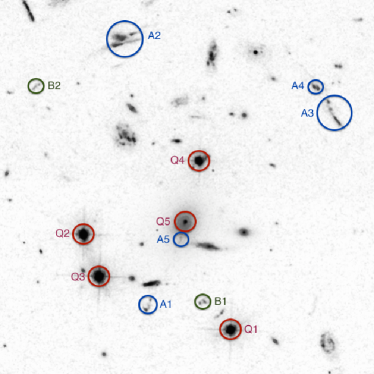
The Q system is natural for time-delay measurements. Two of the four possible time delays (between Q1-Q2 and Q1-Q3) of the quasar images have been measured (Fohlmeister et al., 2007, 2008) and a third is expected. The image separation is large (up to $14^{\prime\prime}$), and since time delays scale with the square of the image separation, the time delays are much longer than with galaxy lenses. Image Q3 lags the nearby Q2 by 40 days and lags Q1 by 821 days. The cluster gas has also been observed in X-rays (Ota et al., 2006). As data have accumulated, many different models have been published (Oguri et al., 2004; Williams & Saha, 2004; Kawano & Oguri, 2006; Saha et al., 2007; Inada et al., 2008; Liesenborgs et al., 2009; Oguri, 2010).

Figure 2: The reference model (equation 6) using all the data constraints. Density (left panel) means projected density in $\rm kg\,m^{-2}$ and potential (right panel) is $t_{\rm grav}$ in years. Lensed images and cluster galaxies are marked.

3 Time delays in lensing

Let us briefly recall the physics of time delays. This is conveniently done using Fermat’s principle as applied to gravitational lensing (Blandford & Narayan, 1986). Consider a sky-projected density $\Sigma(\vec{x})$ at redshift $z_{L}$. Here $\vec{x}$ represents the physical (not comoving) coordinates perpendicular to the line of sight. The gravitational time delay due to this mass will be

$$\nabla^{2}t_{\rm grav}=-(1+z_{L})\frac{8\pi G}{c^{3}}\,\Sigma(\vec{x}\,)\,.$$ (1)

Now consider a source at $\vec{x}_{s}$. A light ray coming from this source, being deflected at the lens so that it heads to the observer, will have an additional geometrical time delay of

$$t_{\rm geom}=\frac{(1+z_{L})}{2c}\frac{d_{S}}{d_{L}d_{LS}}\left|\vec{x}-\vec{x}_{s}\right|^{2}$$ (2)

where the $d_{L}$ is the angular-diameter distance to the lens, and $d_{S}$ and $d_{LS}$ are angular diameter distances from observer to source and from lens to source respectively. In a flat cosmology

$$d_{z_{1},z_{2}}=\frac{c/H_{0}}{1+z_{2}}\int_{z_{1}}^{z_{2}}\frac{dz}{\sqrt{\Omega_{m}(1+z)^{3}+\Omega_{\Lambda}}}$$ (3)

gives the various angular-diameter distances.

The total time delay is then

$$t(\vec{x},\vec{x}_{s})=t_{\rm geom}(\vec{x},\vec{x}_{s})+t_{\rm grav}(\vec{x})\,.$$ (4)

Images will form where $t(\vec{x},\vec{x}_{s})$ has a minimum, saddle point, or maximum. The tensor magnification is the inverse matrix of second derivatives of $t(\vec{x})$. Note that the dependence on $\vec{x}_{s}$ has been differentiated out. Flexion consists of the derivatives of the tensor magnification, hence third derivatives of the time.

Lens modelling consists of reconstructing $\Sigma(\vec{x})$ and $\vec{x}_{s}$. For a quasar source, $\vec{x}_{s}$ is a single point, for an extended source a superposition of source points must be considered. The earliest detailed lens models (Young et al., 1981) already noted the non-uniqueness of lens models. Falco et al. (1985) quantified the most important of these, now known as the steepness degeneracy or the mass-sheet degeneracy: steeper mass profiles give longer time delays, while leaving image positions and shapes the same. As modellers explored models further, it turned out that the shape of the mass distribution also affects time delays (Saha & Williams, 1997; Zhao & Qin, 2003; Saha & Williams, 2006). Degeneracies have also been studied theoretically (Schneider & Sluse, 2013). Having sources at multiple different redshifts (high redshift contrast) tends to suppress degeneracies (AbdelSalam et al., 1998; Saha & Read, 2009) but does not eliminate them completely (Liesenborgs et al., 2008; Liesenborgs & De Rijcke, 2012).

It is useful to break down lensing time delays into three factors: lens substructure, lens size and cosmology. The time delay between the innermost and outermost images can be written as

$$\Delta t_{\rm in,out}=f_{\rm lens}\frac{A_{\rm lens}}{A_{\rm sky}}\,\frac{d_{L}d_{S}}{d_{LS}}\quad A_{\rm lens}=\frac{\pi}{4}(\theta_{\rm in}+\theta_{\rm out})^{2}.$$ (5)

Cosmology enters through the distance factors, while $A_{\rm lens}$ is the size of the lens on the sky, and is fixed by the astrometry. With these factors fixed, $f_{\rm lens}$ is the remaining dependence on substructure. Typical values are 2–6 for systems with 2+1 images, and 0.5–2 for systems with 4+1 images (Saha et al., 2006). That is to say, substructure is very important for time delays. This dependence is undesirable when estimating cosmological parameters, but it is welcome for inferring substructure.

4 Isolating the time-delay modes

In this section we produce a form of principal components analysis (PCA) to isolate the information that time delays provide on the mass distribution, assuming the cosmological parameters are known. A somewhat related technique, for lensing clusters with multiple source redshifts but not necessarily including time delays, is developed by Lubini et al. (2014).

We reconstruct the mass distribution in two ways: first, including the measured time delays (say TD models), and second, with no time-delay information (say NTD models). For each of TD and NTD, we reconstructed an ensemble of mass maps (30 in number). Each mass map is on a grid (size $74\times 74$).

We now wish to find the variation present in the NTD ensemble but not in the TD ensemble. This will provide information on substructure possibilities left by image data (only) but ruled out by time delays. Let $X_{n}^{i}$ denote the projected density of the $i$th TD model ($i$ going from 1 to 30 in this paper) at the $n$th grid point (of $74^{2}=5476$ grid points). Similarly use $Y_{n}^{i}$ for the NTD mass maps. Next, we choose a reference $Z_{n}$,

$$Z_{n}=\langle X_{n}^{i}\rangle$$ (6)

which is the ensemble average of the TD maps. Then

$$\Delta X_{n}^{i}=X_{n}^{i}-Z_{n}$$ (7)

is the ensemble variation about the reference. Then we introduce a moment matrix

$$M_{mn}(X)=\left\langle\Delta X_{m}^{i}\,\Delta X_{n}^{i}\right\rangle$$ (8)

where the average is again over the TD maps. $M_{mn}(X)$ is just the covariance between pairs of grid points. The eigenvalues and eigenvectors of $M_{mn}(X)$ describe how sets of grid points tend to vary together. Let us denote them by $\lambda_{k}(X)$, and $V_{n}^{k}(X)$ respectively; the superscript $k$ denotes the $k$th eigenvalue and eigenvector ($k=1$ having the largest eigenvalue). In practice, the first few eigenvalues dominate. The vector

$$Z_{n}\pm\sqrt{|\lambda_{k}(X)|}\,V_{n}^{k}(X),$$ (9)

displayed as a density map, shows the principal mode of variation of the mass model. (There is no sum over $k$.) These variation modes are, of course, orthogonal.

We then proceed to the NTD maps. Let these be $Y^{i}_{n}$ and let

$$\Delta Y_{n}^{i}=Y_{n}^{i}-Z_{n}$$ (10)

be the variations with respect to the reference model. We now subtract off the variation modes of TD mass maps

$$\Delta\bar{Y}_{n}^{i}=\Delta Y_{n}^{i}-\sum_{k}\left({\textstyle\sum_{m}}\Delta Y^{i}_{m}V_{m}^{k}(X)\right)V_{n}^{k}(X)$$ (11)

leaving variations that are orthogonal to the TD variations. Using these, we build another moment matrix

$$M_{mn}(Y)=\left\langle\Delta\bar{Y}_{m}^{i}\,\Delta\bar{Y}_{n}^{i}\right\rangle.$$ (12)

The eigenvalues and eigenvectors of $M_{mn}(Y)$ contain the modes present in NTD maps models but absent from the TD maps. These modes can be conveniently displayed as

$$Z_{n}\pm\sqrt{|\lambda_{k}(Y)|}\,V_{n}^{k}(Y).$$ (13)

We call these “variations ruled out by the time delays” and these are the main results of this paper. One sign of the $\pm$ must be chosen for definiteness, but it does not matter which one.

Figure 3: Time delay estimates using TD models (upper) and NTD models (lower). TD2, TD3, TD4 and TD5 (or NTD2, NTD3, NTD4, NTD5) are the time delays for image Q2, Q3, Q4 and Q5 respectively with respect to Q1. Vertical dashed lines show the input time delays from Fohlmeister et al. (2008).

5 Application to SDSS J1004+4112

The mass distribution $\Sigma(\vec{x})$ can be reconstructed in different ways: Oguri (2010) uses a parametrized form, Saha et al. (2007) built it out of mass tiles or pixels, while Liesenborgs et al. (2009) used an adaptive superposition of Plummer components. The latter, and in particular the GRALE code, is used in the present work.

5.1 Mass reconstruction using GRALE

As mentioned above, GRALE (Liesenborgs et al., 2006, 2007, 2009) makes free-form mass models for the lensing cluster, as a superposition of many Plummer lenses. Except for the redshift and general location, no information from the lens itself is used. The inversion input consists of (1) lensed-image positions and source redshifts, (2) regions where additional images have not been identified but could be present, and (3) time delays if any. Each of these is used to define a fitness measure of a mass distribution.

• For a given mass map, the input multiple images are ray-traced back to the source plane. The ‘overlap fitness’ of the mass map expresses how well these back-projected images overlap. It is important to consider fractional overlap rather than simple source-plane distances to avoid favouring extreme magnification (tiny sources).

• The back-projection may give rise to extra images. If they are not in regions specified by the modeller as allowed, they are spurious. These penalize the mass map through a ‘null fitness’ measure. Through the null fitness, GRALE uses the non-occurrence of images at random locations as useful data.

• The ‘time-delay’ fitness measures how well the time delay in a mass distribution agrees with the observations.

GRALE uses a multi-objective genetic algorithm to find free-form mass maps which provide optimal fits to the data according to the above criteria. If more Plummer-lens components are allowed, the fitness will tend to be better. Accordingly, we used a heuristic Occam’s-razor criterion to find a compromise between better fitness and more components (Mohammed et al., 2014a). This effect sets the resolution adaptively. No additional priors or regularization are used.

5.2 Mass models

Our mass maps for SDSS J1004+4112 were of two kinds, as follows.

• No time delay (or NTD) models. We used the three image systems (Q, A and B; total 12 images), but gave no time-delay information in this case. GRALE finds an optimal solution, restricting extra images using the technique of null spaces, for this dataset. We repeated the same procedure 30 times to generate a statistical ensemble of 30 models.

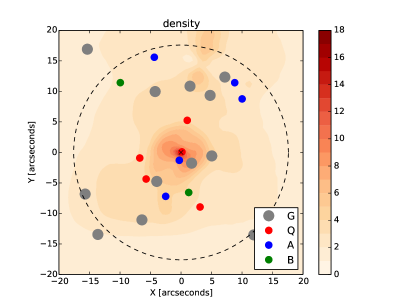
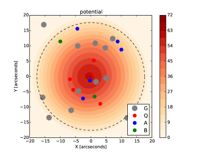
• Time delay (or TD) models. For these we used the same data set, plus the two measured time delays: 40 days in Q2–Q3 and 821 days in Q1–Q3 (see Figure 1). Following the same procedure, we made an ensemble of 30 mass maps. Figure 2 shows the ensemble average of the TD models, which is used as the reference $Z_{n}$ from Section 4. The left panel of Figure 2 shows the projected density and the right panel shows the potential in the colour code. This mass distribution shows slight differences from Liesenborgs et al. (2009), because the present work uses an adaptive resolution scheme, but these differences do not appear to be significant.

The method described in Section 4 is then applied to the TD and NTD models. Tests in Mohammed et al. (2014a) indicate that GRALE ensembles of this size underestimate the actual uncertainties by a factor of two, but do explore the different uncertainties. Thus, the eigenvalues reported below are certainly underestimates, but the eigenvectors should be a good representation of the variation.

Figure 4: Distribution of eigenvalues $\lambda_{k}(X)$ and $\lambda_{k}(Y)$, labelled as TD and NTD respectively, ranked by absolute value.

Figure 5: The main/largest variation in surface density ruled out by time delays (upper panel). The red and the blue color bars represents positive and negative values (in $\rm kg\,m^{-2}$) respectively. The two lower panels show the second and third largest variation ruled out by time delays.

Figure 6: The main/largest variation ruled out by time delays. The red and the blue colour bars represents positive and negative values (in years) respectively.

5.3 Results and interpretation

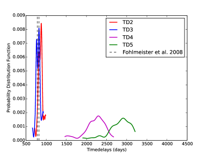
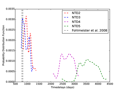
Figure 3 shows the distribution of time delays in the TD and NTD ensembles. As expected in the TD models, the first two time delays, which were also used as data inputs, show little variation (though larger than the observational uncertainties) while the other two show large variations. In the NTD models, all the time delays show large variations. Most of the TD models also favour lower time delays for Q4 and Q5, as compared to the NTD models estimate. Thus, existing time-delay measurements constrain future measurements to some degree, but not very tightly, indicating that future measurements will bring substantial new information.

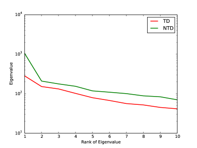
Figure 4 shows the eigenvalues of the NTD and TD modes. The largest NTD mode evidently dominates, being a factor of five larger than the second largest mode. When time delays are included, it is also the case that one TD mode is much larger than the rest.

Figure 7: Variation of enclosed mass of the reference model around the largest NTD mode (shown in Figure 5) as a function of projected radius. Linear scales on the left, log scales on the right.

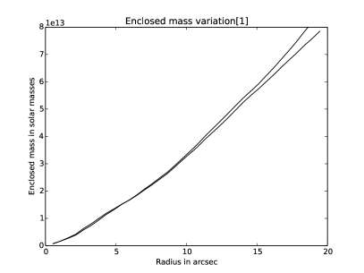
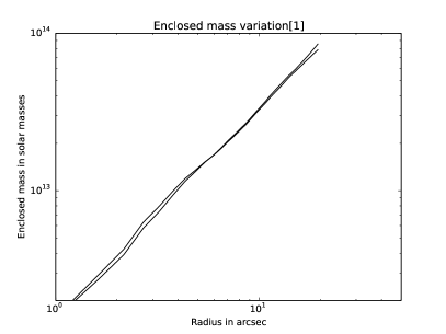
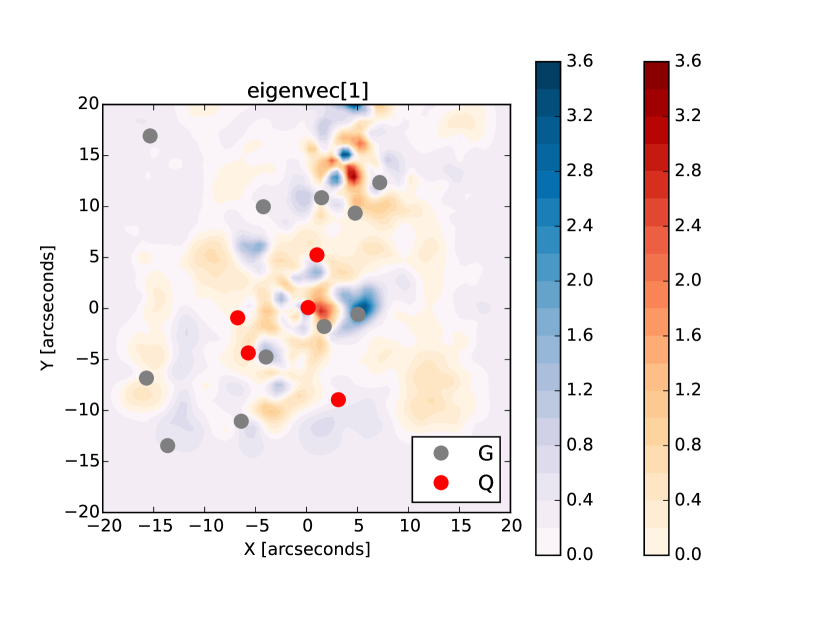
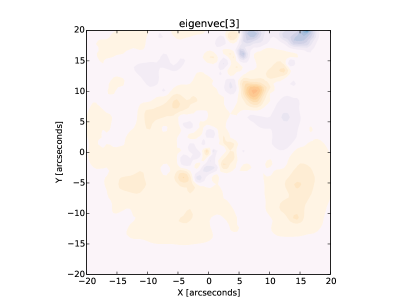
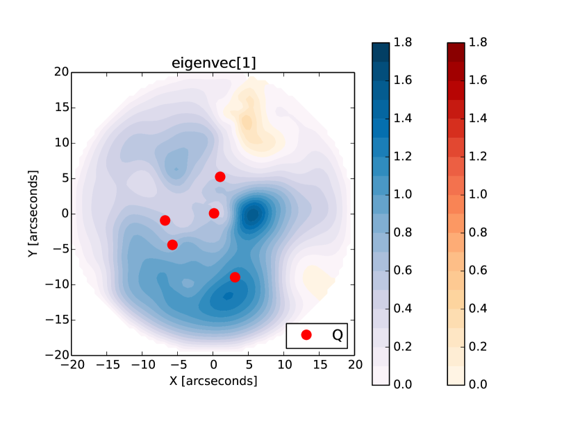
Figure 5 presents the main result of this paper. It illustrates the largest NTD variation mode that is absent in the TD ensemble (cf. equation 13), in other words, the largest variations ruled out by the time-delay measurements. The upper panel of the figure shows the eigenvector corresponding to the largest eigenvalue. The two central blobs in the upper panel of Figure 5 (blue and red, hence anti-correlated) allow the mass to shift the local mass peak towards or away from the cluster centre, and hence change the steepness of the mass profile. Without the TD constraints, the central peak of the mass distribution can be more lopsided, whereas the TD constraints force the central peak to be rounder. The rather large uncertainties (20%–40% in $\Sigma$) in the central region of the NTD models is reduced in the TD models. This local uncertainty of 20%–40% is, however, less than 1% of the total mass in the strong-lensing region. That is to say, time delays are constraining substructures that are only a percent of the total. The red and blue blobs also are in the vicinity of the two galaxies in the very central region. That may be coincidental, but it is worth remarking that the mass in the blobs is of the order of a galaxy-halo mass, such as may be tidally stripped from a galaxy near the centre of a cluster. This suggests that time delays may give very sophisticated information about the variation of the mass near the environment of the galaxies in the central region, or in other words, about the sub-structures in a dense environment. Therefore, the third time-delay, which is expected for the image Q4, could be very useful in extracting the substructure information of the cluster near its centre. Note that this interesting region is not accessible through the more well-known techniques of weak lensing and flexion.

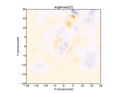
The lower two panels of Figure 5 shows the second and third largest variation modes. These variations modes are weaker, also evident from Figure 4 as all other eigenvalues after the first one are sub-dominant. The number of non-zero eigenvalues for NTD should equal the number of time-delay measurements (two in this case), but in practice further modes are present, and only gradually die away. These are basically noise modes, which exist because we have only 30 models for our principal-components analysis. (Numerical noise due to round-off error in the matrix operations is negligible.)

Upon measuring the short Q2-Q3 time delay Fohlmeister et al. (2007) already noted that substructure would be necessary to account for their observation. We have not considered separately the case where only this one time delay is known. We see in Figure 4, however, that only one of the NTD eigenvalues is larger than the TD eigenvalues, indicating that only one of the measured time delays (surely the longer Q1-Q3 value) gives a substructure constraint. This does not mean that the Q2-Q3 measurement can be explained without substructure; only that the measurement on its own is not constraining what that substructure could be.

Figure 6 shows the variation in lens potential $t_{\rm grav}$ corresponding to the density variation from the main panel in Figure 5. Here we can see the effect of measuring the delays between Q1, Q2, and Q3. The NTD models have $t_{\rm grav}$ between Q1 and Q2 varying by about 0.5 years, that is, varying by 25% of the measured value. Between Q2 and Q3, the time delay varies by about 0.3 years in the NTD models, which is more than twice the measured delay between this pair. Between Q3 and Q4 there is little variation. This does not mean that the NTD models have little variation in the Q3–Q4 delay; it just means that similar variation is present in the TD models, and hence not ruled out by the Q1–Q2–Q3 measurements. All this is what one would have expected from Figure 3. Surprising, however, is that the largest variation ruled out by the time delays is the blob $5^{\prime\prime}$ west of the cluster centre, not near any of the images.

Figure 7 shows the enclosed mass and its variation. The enclosed mass is comparable with Figure 3 of Oguri (2010), as expected. As also evident from figure 5, the NTD mode is not like a global change of steepness — the steepness appears to have been already constrained by the image data, because of the redshift contrast between the Q, A and B systems. So the time delays are giving us information not on the steepness but about the shape of the profile. The NTD models allow for strongly E/W ellipticity in the central region, changing to a more N/S elongation further out, but the time delays force the model to be rounder and less lopsided.

6 Discussion

This paper expresses the information that comes from lensing time delays in a way that is orthogonal to other lensing observables. We used the cluster SDSS J1004+4112 because of the richness of strong-lensing information. SDSS J1029+2623 (Fohlmeister et al., 2013; Oguri et al., 2013) would also be interesting for a similar study, as would MACS J1149+2223 (Kelly et al., 2014; Oguri, 2014) if time delays for the recently-discovered supernova can be measured. The main results are shown in figures 5 and 6. The interpretation is very preliminary, because a new time delay is expected soon, but nonetheless shows two interesting features.

First, it is remarkable how a small mass redistribution can produce a large difference in time delays. As Figure 5 shows, the main mass-redistribution ruled out by the two published time delays is a small blob that is only $\sim 1\%$ of the total mass in the strong-lensing region, and yet this redistribution can change a time delay by 50%. It appears that time delays are providing substructure constraints at the 1% level.

Second, the mass redistribution is not mainly near the images, but mainly in another region of the cluster. Overall, the time delays reduce the allowed lopsidedness of the cluster, but it is intriguing that the main redistribution appears to shift mass from the neighbourhood of one cluster galaxy to the vicinity of another cluster galaxy.

The expected third time-delay measurement in this cluster will be very interesting. As seen in Figure 1, the two time delays we used in our analysis are between Q1–Q2 and Q1–Q3. All of these images are towards the west and south-east of the cluster. The new measurement would involve Q4, which lies to the north.

So, we conclude that strong lensing with time delays provides important constraints on the distribution of matter near the centre of the lensing cluster, regions not accessible to weak lensing or flexion. Additionally, time delays may provide new information on the distribution of matter in the densest regions of clusters and indirectly on the role of AGN feedback, adiabatic contraction, and other dynamical processes.

References

- Abdelsalam et al. (1998) Abdelsalam H. M., Saha P., Williams L. L. R., 1998, MNRAS, 294, 734
- AbdelSalam et al. (1998) AbdelSalam H. M., Saha P., Williams L. L. R., 1998, AJ, 116, 1541
- Blandford & Narayan (1986) Blandford R., Narayan R., 1986, ApJ, 310, 568
- Blumenthal et al. (1986) Blumenthal G. R., Faber S. M., Flores R., Primack J. R., 1986, ApJ, 301, 27
- Coles (2008) Coles J., 2008, ApJ, 679, 17
- Dehnen (2005) Dehnen W., 2005, MNRAS, 360, 892
- Falco et al. (1985) Falco E. E., Gorenstein M. V., Shapiro I. I., 1985, ApJL, 289, L1
- Fohlmeister et al. (2008) Fohlmeister J., Kochanek C. S., Falco E. E., Morgan C. W., Wambsganss J., 2008, ApJ, 676, 761
- Fohlmeister et al. (2007) Fohlmeister J. et al., 2007, ApJ, 662, 62
- Fohlmeister et al. (2013) Fohlmeister J., Kochanek C. S., Falco E. E., Wambsganss J., Oguri M., Dai X., 2013, ApJ, 764, 186
- Gnedin et al. (2004) Gnedin O. Y., Kravtsov A. V., Klypin A. A., Nagai D., 2004, ApJ, 616, 16
- Halkola et al. (2008) Halkola A., Hildebrandt H., Schrabback T., Lombardi M., Bradač M., Erben T., Schneider P., Wuttke D., 2008, A&A, 481, 65
- Hammer (1991) Hammer F., 1991, ApJ, 383, 66
- Inada et al. (2008) Inada N., Oguri M., Falco E. E., Broadhurst T. J., Ofek E. O., Kochanek C. S., Sharon K., Smith G. P., 2008, PASJ, 60, L27
- Inada et al. (2005) Inada N. et al., 2005, PASJ, 57, L7
- Inada et al. (2003) Inada N. et al., 2003, Nature, 426, 810
- Kawano & Oguri (2006) Kawano Y., Oguri M., 2006, PASJ, 58, 271
- Kelly et al. (2014) Kelly P. L. et al., 2014, ArXiv e-prints, 1411.6009
- Kneib (2002) Kneib J.-P., 2002, in The Shapes of Galaxies and their Dark Halos, Natarajan P., ed., pp. 50–57
- Liesenborgs & De Rijcke (2012) Liesenborgs J., De Rijcke S., 2012, MNRAS, 425, 1772
- Liesenborgs et al. (2006) Liesenborgs J., De Rijcke S., Dejonghe H., 2006, MNRAS, 367, 1209
- Liesenborgs et al. (2007) Liesenborgs J., De Rijcke S., Dejonghe H., Bekaert P., 2007, MNRAS, 380, 1729
- Liesenborgs et al. (2008) Liesenborgs J., De Rijcke S., Dejonghe H., Bekaert P., 2008, MNRAS, 386, 307
- Liesenborgs et al. (2009) Liesenborgs J., De Rijcke S., Dejonghe H., Bekaert P., 2009, MNRAS, 397, 341
- Lubini et al. (2014) Lubini M., Sereno M., Coles J., Jetzer P., Saha P., 2014, MNRAS, 437, 2461
- Martizzi et al. (2013) Martizzi D., Teyssier R., Moore B., 2013, MNRAS, 432, 1947
- Mashchenko et al. (2006) Mashchenko S., Couchman H. M. P., Wadsley J., 2006, Nature, 442, 539
- Mohammed et al. (2014a) Mohammed I., Liesenborgs J., Saha P., Williams L. L. R., 2014a, MNRAS, 439, 2651
- Mohammed et al. (2014b) Mohammed I., Martizzi D., Teyssier R., Amara A., 2014b, ArXiv e-prints
- Navarro et al. (1997) Navarro J. F., Frenk C. S., White S. D. M., 1997, ApJ, 490, 493
- Oguri (2007) Oguri M., 2007, ApJ, 660, 1
- Oguri (2010) Oguri M., 2010, PASJ, 62, 1017
- Oguri (2014) Oguri M., 2014, ArXiv e-prints, 1411.6443
- Oguri et al. (2004) Oguri M. et al., 2004, ApJ, 605, 78
- Oguri et al. (2013) Oguri M. et al., 2013, MNRAS, 429, 482
- Ota et al. (2006) Ota N. et al., 2006, ApJ, 647, 215
- Paraficz & Hjorth (2010) Paraficz D., Hjorth J., 2010, ApJ, 712, 1378
- Rathna Kumar et al. (2014) Rathna Kumar S., Stalin C. S., Prabhu T. P., 2014, ArXiv:1404.2920
- Read & Gilmore (2005) Read J. I., Gilmore G., 2005, MNRAS, 356, 107
- Refsdal (1964) Refsdal S., 1964, MNRAS, 128, 307
- Refsdal (1966) Refsdal S., 1966, MNRAS, 132, 101
- Saha et al. (2006) Saha P., Coles J., Macciò A. V., Williams L. L. R., 2006, ApJL, 650, L17
- Saha & Read (2009) Saha P., Read J. I., 2009, ApJ, 690, 154
- Saha & Williams (1997) Saha P., Williams L. L. R., 1997, MNRAS, 292, 148
- Saha & Williams (2006) Saha P., Williams L. L. R., 2006, ApJ, 653, 936
- Saha et al. (2007) Saha P., Williams L. L. R., Ferreras I., 2007, ApJ, 663, 29
- Schaller et al. (2014) Schaller M. et al., 2014, ArXiv e-prints
- Schneider & Sluse (2013) Schneider P., Sluse D., 2013, A&A, 559, A37
- Sereno & Paraficz (2014) Sereno M., Paraficz D., 2014, MNRAS, 437, 600
- Sharon et al. (2014) Sharon K., Gladders M. D., Rigby J. R., Wuyts E., Bayliss M. B., Johnson T. L., Florian M. K., Dahle H., 2014, ApJ, 795, 50
- Sharon et al. (2005) Sharon K. et al., 2005, ApJL, 629, L73
- Suyu et al. (2014) Suyu S. H. et al., 2014, ApJL, 788, L35
- Teyssier et al. (2013) Teyssier R., Pontzen A., Dubois Y., Read J. I., 2013, MNRAS, 429, 3068
- Williams & Saha (2004) Williams L. L. R., Saha P., 2004, AJ, 128, 2631
- Young et al. (1981) Young P., Gunn J. E., Oke J. B., Westphal J. A., Kristian J., 1981, ApJ, 244, 736
- Zhao & Qin (2003) Zhao H., Qin B., 2003, ApJ, 582, 2