CERN PH-TH/2014-254
Hamiltonian Truncation Study of the Theory
in Two Dimensions
Slava Rychkova,b,c, Lorenzo G. Vitaled
a CERN, Theory Division, Geneva, Switzerland
b Laboratoire de Physique Théorique de l’École normale supérieure, Paris, France
c Faculté de Physique, Université Pierre et Marie Curie, Paris, France
d Institut de Théorie des Phénomènes Physiques, EPFL, CH-1015 Lausanne, Switzerland
Abstract
We defend the Fock-space Hamiltonian truncation method, which allows to calculate numerically the spectrum of strongly coupled quantum field theories, by putting them in a finite volume and imposing a UV cutoff. The accuracy of the method is improved via an analytic renormalization procedure inspired by the usual effective field theory. As an application, we study the two-dimensional theory for a wide range of couplings. The theory exhibits a quantum phase transition between the symmetry-preserving and symmetry-breaking phases. We extract quantitative predictions for the spectrum and the critical coupling and make contact with previous results from the literature. Future directions to further improve the accuracy of the method and enlarge its scope of applications are outlined.
December 2014
1 Introduction
How do we extract predictions about a strongly coupled quantum field theory (QFT) which is not exactly solvable? The lattice would be one answer, but it’s not the only one. Hamiltonian truncation techniques, which generalize the Rayleigh-Ritz method familiar from quantum mechanics, are a viable deterministic alternative to the lattice Monte Carlo simulations, at least for some theories. These techniques remain insufficiently explored, compared to the lattice, and their true range of applicability may be much wider than what is currently believed. There exist several incarnations of Hamiltonian truncation, some better known than others, differing by the choice of basis and of the quantization frame. For example, Discrete Light Cone Quantization (DLCQ) [2] and Truncated Conformal Space Approach (TCSA) [3] are two representatives of this family of methods.
Here we will be concerned with what is perhaps the simplest setting for the Hamiltonian truncation—the theory in two spacetime dimensions. Moreover, we will consider the most straightforward realization of the method—we will quantize at fixed time rather than on the light cone, and use the Fock space basis for the Hilbert space rather than the abstruse conformal bases.111The use of a conformal basis in two dimensions requires compactifying the scalar field [4], see the discussion in section 4.5. We will expand the Hamiltonian into ladder operators, as on the first page of every QFT textbook. We will however take this Hamiltonian more seriously than in most textbooks. Namely, we will use it to extract non-perturbative predictions, rather than as a mere starting point for the perturbative calculations. Concretely, we will (1) put the theory into a (large) finite volume, to make the spectrum discrete, (2) truncate the Hilbert space to a finite dimensional subspace of low-energy states, and (3) diagonalize the truncated Hamiltonian numerically.
In spite or perhaps because of its extreme simplicity, this concrete idea has so far received even less attention than its more sophisticated cousins mentioned above. The only prior works known to us are [5, 6].222A more extensive description of this work can be found in [7] and [8]. Another paper [9] studied the two-dimensional Yukawa model without scalar self-interaction. Here, we will follow up on these early explorations with our own detailed study.
While the basic idea and the qualitative conclusions of our work will be similar to [5, 6], our implementation contains several conceptual and technical novelties. In particular, we will pay special attention to the convergence rate of the method, and will develop analytical tools allowing to accelerate the convergence, improve the accuracy, and better understand the involved systematic errors.
The advances reported in this paper, as well as the ongoing progress in developing the other variants of the Hamiltonian truncation [10, 11, 12], [13, 14, 1] make us hopeful that in a not too distant future these methods will turn into precision tools for studying strongly coupled QFTs.
The structure of the paper is clear from the table of contents. In section 2 we present the problem and the basic methodology used to study the spectrum numerically.
Section 3 elucidates the ideas behind the renormalization procedure, its implementations adopted in the numerical study, and provides some tests of the analytical results. The reader afraid of the technicalities may skip it. Yet it is precisely this section which is the theoretical heart of the paper.
Section 4 contains the main numerical application of the work, i.e. the calculation of the spectrum of the two-dimensional theory. The dependence of the numerical results on the physical and unphysical parameters is analyzed carefully, and an estimate of the critical coupling is provided. Computations were performed using a python code included with the arXiv submission.
In section 5 we compare our method to the existing ones in the literature. Most of these prior studies focused in particular on the critical coupling estimates.
We conclude in section 6. Appendix A presents some technical details useful for the practical implementation of the procedure. Appendix B provides the perturbative checks of our method, alongside a discussion of the Borel-summability of the model.
We would like to mention right away that this paper was developed in parallel with Ref. [1] published three months ago and devoted to the TCSA approach in dimensions. The concrete example treated in [1] was the theory in dimensions, which has the same phase structure as the case studied here. The attentive reader will notice many similarities in section 4 regarding the physics discussion, and in section 3 regarding the renormalization procedure. However, concerning the latter, there is also a difference of principle which will be stressed in section 3.5 below.
2 The problem and the method
2.1 Hamiltonian
We will be studying the two-dimensional theory, defined by the following Euclidean action:
| (2.1) | |||
| (2.2) |
Here denotes normal ordering. Normal ordering of the free massive scalar action simply means that we set to zero the ground state energy density (in infinite flat space, and before adding the quartic perturbation). The quartic interaction term is then assumed normal-ordered with respect to the mass appearing in the free action. In perturbation theory this simply corresponds to forbidding the diagrams with lines beginning and ending inside the same quartic vertex. In terms of operators, this means that we are adding counterterms [15]:
| (2.3) |
Here
| (2.4) |
is a logarithmically UV-divergent quantity.
Although absent in (2.1), below we will also need to consider perturbations given by the normal-ordered operator:
| (2.5) |
The above equations specify what we mean by the theory in infinite flat space, and also define the mass parameter and the quartic coupling in terms of which we will parametrize the theory. All physical quantities (such as particles masses and S-matrix elements) are then finite functions of and . Also the change of the ground state energy density due to turning on the coupling is finite and observable in this theory. This change can be thought of as the contribution of the theory (2.1) to the cosmological constant.
Since both and are dimensionful, physics depends on their dimensionless ratio , while (or ) sets the overall mass scale. We will assume to have a stable vacuum. Both signs of are interesting, but in this paper we will only consider the case . Notice that this does not mean that we will always be in the phase of preserved symmetry , since the mass parameter undergoes renormalization. In fact, as we will see below, for and the theory finds itself in the phase where the symmetry is spontaneously broken. This is a nonperturbative phenomenon. For , the fate of the symmetry is of course determined by the sign of .
In this paper we will study the above theory not in infinite space but on a cylinder of the form , where is the circle of length and will be thought of as Euclidean time. We will impose the periodic boundary conditions around the circle. We will describe the theory on this geometry in the Hamiltonian formalism, taking advantage of the fact that the finite volume spectrum is discrete.
Now, what is the Hamiltonian which describes the theory (2.1) on ? The correct answer to this question involves a subtlety, so let us proceed pedagogically.
We first discuss the Hamiltonian which describes the free massive scalar. In canonical quantization, the field operator is expanded into modes:
| (2.6) |
where the momenta take discrete values , , , and the ladder operators satisfy the usual commutation relations:
| (2.7) |
The Hilbert space of the theory is the Fock space of these ladder operators, spanned by the states
| (2.8) |
where is the normalization factor to get a unit-normalized state. The free scalar Hamiltonian is then given by:
| (2.9) |
The only subtlety here is the c-number term . The point is that we want the oscillator part of the finite volume Hamiltonian to be normal-ordered. However, the normal ordering counterterm in infinite space and for finite is slightly different, and compensates for this mismatch. It is nothing but the Casimir energy of the scalar field, and is given by (see [16]):
| (2.10) |
This expression can be derived in many equivalent ways. One method is to regulate the difference of the zero-point energies:
| (2.11) |
Another method is to compute the partition function of the theory on the torus , which can be done from the path integral formulation of the theory. The partition function defined in this way enjoys the property of modular invariance. This method naturally produces a term in the free energy of the form .
We next discuss the finite-volume Hamiltonian for the interacting theory. It will have the form:
| (2.12) | |||
| (2.13) |
The normal ordering here is defined on the circle of length in the Hamiltonian sense, just putting all creation operators to the left. Thus:
| (2.14) |
The origin of the terms in (2.12) lies again in the fact that the normal-ordering counterterms added when defining ,
| (2.15) |
are not exactly the same as in the infinite space definition (2.3). The difference is
| (2.16) |
where in the second equality we used .
To compute we rewrite in the form adapted to the Hamiltonian quantization:
| (2.17) |
The difference is finite and is readily calculated using the Abel-Plana formula:
| (2.18) |
This allows us to complete the terms in (2.12). Thus, the Hamiltonian on a circle of finite length corresponding to the infinite space theory (2.3) is given by:
| (2.19) | |||
| (2.20) |
We see that the Hamiltonian (2.19) differs from the “naive” Hamiltonian
| (2.21) |
by “correction terms”, proportional to and . The presence of these terms is conceptually important. They would be also straightforward to include into numerical analysis, for any . However, in this paper we will be focussing on the case . In this regime the corrections due to and are exponentially suppressed, and their numerical impact is negligible. For this reason, and to simplify the discussion, we will omit the exponentially suppressed corrections. With this proviso, from now on we will use the “naive” Hamiltonian (2.21).
2.2 Truncation
We next explain the truncation method. We will work in the Hilbert space spanned by the free massive scalar states. The Hamiltonian acts in this space, and the problem is to diagonalize it. We thus use the free massive scalar states as a basis into which we expand the eigenstates of the interacting theory. Let us think of the Hamiltonian as an infinite matrix where numbers the states in :
| (2.22) |
Notice that the states as introduced above form an orthonormal basis of . To find the spectrum of the theory in finite volume, we need to diagonalize the matrix . This diagonalization can be done separately in sectors having fixed quantum numbers corresponding to the operators commuting with the Hamiltonian.
The first such quantum number is the momentum: . In this paper we will be working in the sector of states of vanishing total momentum:
| (2.23) |
In a large volume, the states of nonzero momentum should correspond to boosted zero-momentum states, and their energies should be related to zero-momentum energies by the Lorentz-invariant dispersion relation. It would be interesting to check this in future work.
The second conserved quantum number is the spatial parity , which acts . It maps the state (2.8) into . In this paper we will be working in the -invariant sector,333The extension of our method to the -odd sector is straightforward. We consider only the -even sector, because we do not expect bound states with . whose orthonormal basis consists of the states
| (2.24) |
where is the normalization factor:
| (2.25) |
The restriction to the subspace will be tacitly assumed in all of the rest of the paper.
The final conserved quantum number is the already mentioned global symmetry (the field parity). Its eigenvalue on the states (2.8) is . Below we will be considering both the -even and -odd sector.
Each of the two sectors still contains infinitely many states. We will thus have to truncate the Hilbert space. The truncation variable will be the -eigenvalue:
| (2.26) |
We will truncate by considering all states of . The parameter should be thought of as a UV cutoff. The truncated Hilbert space is finite-dimensional, and the matrix restricted to this space can be diagonalized numerically. This is what we will do.
In principle, one could imagine alternative truncation schemes. For example, one can truncate in the maximal wavenumber . Such a truncation would be closer to the usual way one implements the UV cutoff in field theory. By itself, however, it does not render the Hilbert space finite-dimensional. One could also think of truncating in the total occupation number of the state, or in the individual occupation numbers per oscillator, and so on. Our initial exploration of such subsidiary cutoffs did not produce any dramatic gains in the performance of the method. In the end we decided to stick to the cutoff in . As we will see in the next section, this cutoff allows for a natural implementation of the renormalization of the Hamiltonian, necessary to improve the convergence of the method. In the future it may be interesting to return to the other cutoffs, and explore them more systematically.
3 UV cutoff dependence and renormalization
3.1 General remarks
It is not difficult to write a code which computes the matrix restricted to the subspace444See appendix A for some tricks speeding up this computation. and diagonalizes it. The results of these numerical calculations will be discussed below. As we will see, as the UV cutoff is increased, the energy levels computed using the truncated Hilbert space (‘truncated energy levels’) tend to some finite limits. These limits should be naturally identified with the exact energy levels. An interesting theoretical question then arises: what is the convergence rate of the method? There is also a related practical question: how can the convergence be improved? These questions will be discussed in this section.
By calculating the truncated energy levels we are discarding the contribution to the low-energy physics coming from the high energy states of the Hilbert space. Since the UV divergences have been already taken care of, this contribution is power-suppressed and goes to as the cutoff is increased. In the standard Wilsonian approach to the renormalization group, by integrating out high-momentum (or short-distance) degrees of freedom one gets a flow in the space of Hamiltonians, along which the same physics is described in terms of low-momentum degrees of freedom with renormalized couplings. We would like to apply the same philosophy to our case, although we may expect some differences, because our cutoff prescription—cutting off in —is different from the ones normally used in field theory. First of all, it breaks the Lorentz invariance. Second, the fact that we truncate in the total energy of the state, rather than in that of its individual constituents, renders our cutoff effectively non-local. Thus, we should be prepared to see non-local as well as Lorentz-violating operators generated by the flow. We will see, however, that to leading order it will be sufficient to renormalize a few local operators in the Hamiltonian. It will be possible to do this computation in perturbation theory, since the potential we add to the free Hamiltonian is a relevant deformation and becomes less important in the UV. The dimensionless parameter which sets the convergence of the truncated energy levels and the asymptotic magnitude of the counterterms will be . All these considerations will be made concrete in the following.
We start our analysis from the exact eigenvalue equation:
| (3.1) |
where is an infinite-dimensional vector living in the full Hilbert space . Here and below, we use curly to denote energy levels of the interacting theory, while will be used to denote free scalar energy levels.
In our methodology the Hilbert space is divided in two subspaces:
| (3.2) |
where is the low-energy sector of the Hilbert space, treated numerically, while is spanned by an infinite number of discarded high-energy states. So we have , and Eq. (3.1) takes the following form in components:
| (3.3) |
Here we denoted
| (3.4) |
where () is the orthogonal projector on .
Using the second equation in (3.3) to eliminate from the first one, we obtain:
| (3.5) |
or, equivalently,
| (3.6) | |||
| (3.7) |
This equation is very important. Notice that is nothing but the Hamiltonian truncated to the low-energy Hilbert space. Notice furthermore that the mixing between the high and low-energy states is due only to , since is diagonal.
Eq. (3.6) is exact, yet it resembles the truncated eigenvalue equation, with a correction . This equation will be a very convenient starting point to answer the two questions posed at the beginning of this section.
We will now start making approximations. First, we expand in and keep only the zeroth term
| (3.8) |
By dimensional reasons, we expect that the next term in the expansion,
| (3.9) |
will be suppressed with respect to the one we keep by . It will be very interesting to include this term in future work, and we will comment below about how this can be done.
Equation (3.8) defines as an operator on . The definition depends on the eigenvalue that we are trying to compute. This subtlety will be dealt with below, while for the moment let us replace by some reference energy . Even then, the definition seems impractical since it involves a sum over infinitely many states in . Indeed, the matrix elements of according to this definition are given by:
| (3.10) |
Fortunately, in the next section we will give a simplified approximate expression for not involving infinite sums. As we will see, to leading order will be approximated by a sum of local terms:
| (3.11) |
To this leading order, adding to results in simply renormalizing the local couplings. As we will see, a more accurate expression for contains subleading corrections, which in general cannot be expressed as integrals of local operators. The appearance of these nonlocal corrections is due to the above-mentioned fact that truncating in total energy is not a fully local way of regulating the theory.
3.2 Computation of
Consider then the matrix elements (3.10) of for in the truncated basis. We will write them in the form
| (3.12) | |||
| (3.13) |
We are interested in the large- asymptotics for . Of course, for finite the energy levels are discrete and this function should be properly thought of as a distribution (a sum of delta-functions). However, since the high-energy spectrum is dense, the fluctuations due to discreteness will tend to average out when integrating in . Below we will find a continuous approximation for , valid on average. Such an approximation will be good enough for computing the integral in (3.12) with reasonable accuracy. A small loss of accuracy will occur because of the sharp cutoff at ; this will be discussed below in sections 4.3 and 4.4.
Our calculation of will follow the method introduced in [1], section 5.3. It will be based on the fact that the same quantity appears also in the following matrix element:
| (3.14) |
where we inserted a completeness relation in the second step. A word about notation: the Euclidean time dependence of various operators is always meant in the interaction representation, e.g.
| (3.15) |
If the time dependence is not shown, it means that the operator is taken at .
Eq. (3.14) says that is basically the Laplace transform of . The leading non-analytic part of for will come from the leading piece of as . Our method will proceed by first extracting the leading non-analytic part of , and then taking its inverse Laplace transform to get at .
We will present the computation for a general case when the potential contains both and terms:
| (3.16) |
Our Hamiltonian (2.21) has , . Turning on corresponds to an extra contribution to the mass. Having this coupling will be useful for a check of the formalism in section 3.4 below.
We have
| (3.17) |
where we used periodicity and invariance under spatial translations. The non-analyticity of for comes from the integration region where the product of two local operators is singular, i.e. when they are inserted at near-coinciding points. Let us focus on one term in the sum, and rewrite it using Wick’s theorem as:
| (3.18) |
Here is the two-point function of in the free theory on the circle of length . The ’s are integer combinatorial factors (operator product expansion coefficients):
| (3.19) |
In (3.18), the leading non-analytic behavior as will come from the propagator powers . The remaining normal-ordered operators can be Taylor expanded in , :
| (3.20) |
The terms are not shown because they will vanish upon integration. The terms will produce a subleading singularity as . The corresponding contributions to will be suppressed by compared to the leading ones. In this work these subleading contributions will be neglected, but it will be interesting and important to include them in the future.555The subleading contributions will give rise to new, derivative, operators in the Hamiltonian. Since our regulator breaks Lorentz invariance, the derivatives in and are not going to enter symmetrically in these subleading terms.
Eq. (3.20) means that at leading order the correction Hamiltonian will contain terms of the form (3.11) with . To find the couplings , we need to evaluate the non-analytic part of the following quantities:
| (3.21) |
As we will see below, for the behavior will be analytic (for this is a triviality). This implies that only terms will be generated in (3.11).
To evaluate (3.21), we will need a few well-known facts about . In the infinite volume limit the rotation invariance is restored, and the two-point function is a modified Bessel function of the second kind, depending on the distance :
| (3.22) |
It has a logarithmic short distance behavior and decays exponentially at long distances:666 is Euler’s constant.
| (3.23) |
For a finite , the two-point function is obtained from the case via periodization:
| (3.24) |
The periodization corrections are exponentially small for . In our work, this condition will be always satisfied, and so we will use in place of .777The induced error can be estimated by approximating for small . This implies a shift , . For and () the coefficient . This is consistent with having neglected the exponentially suppressed and terms when passing from (2.19) to (2.21).
So we will replace by in (3.21). The non-analytic behavior of the integral comes from the small region, where the short-distance logarithmic asymptotic (3.23) is applicable. To regulate spurious IR divergences, it’s convenient to calculate the first derivative with respect to :
| (3.25) |
where we also replaced by its short-distance asymptotics. The resulting integrals are convergent and readily evaluated:888Mathematica’s Integrate function sometimes gives wrong results for integrals of this type, so be careful.
| (3.26) | |||
modulo errors induced by using the short-distance asymptotics of . These errors are suppressed by . The corresponding corrections to are suppressed by , and will be omitted. Also, as mentioned above, we see that is analytic.
We now have to pass from the small- behavior to the large- asymptotics. Differentiating Eq. (3.14) we have
| (3.27) |
where we defined
| (3.28) |
Thus from the inverse Laplace transforms of we should be able to determine the asymptotics of . These inverse Laplace transforms are found from the following table of direct transforms:
| (3.29) | |||
Since we are only interested in the large- asymptotics, the IR cutoff is not important—its value only influences the analytic parts.
Gathering everything, we obtain the following formula for the leading asymptotic behavior of :
| (3.30) |
where
| (3.31) |
As the notation suggests, the -functions in (3.30) are evaluated at . This equation is the main result of this section. We subjected it to several tests, which we are going to describe below.
Before proceeding, let us comment on the evaluation of the next-to-leading term (3.9) in the renormalization procedure, which will be important in future developments of the method. From this term we will extract the contribution to the coefficients . This correction term is the most interesting of all corrections, since it dominates in the limit . Technically, we should generalize and in Eq. (3.14) to functions of two variables ( and ) and extract the leading non-analytic pieces for . This calculation will involve Wick contractions among the operators in , the cyclic ones being the only nontrivial part.
We shall now move on to the tests of Eq. (3.31).
Test 1
Let us plug (3.30) into (3.12), and do the integral neglecting the dependence on and .999We stress that in numerical computations it will be important to retain these subleading corrections. This gives of the form (3.11), i.e. as a sum of local counterterms with coefficients which are functions of . For example, the part is given by ():
| (3.32) |
This expression was checked as follows. Working in infinite volume, we computed the order perturbative corrections to the vacuum energy, particle mass, and scattering amplitude, imposing the cutoff on the intermediate state energy (thus working in the ‘old-fashioned’ Hamiltonian perturbation theory formalism, rather than in terms of Feynman diagrams). We then checked that the leading dependence of these results is precisely the one implied by (3.32). This way of arriving at (3.32) is more laborious than the one given above, and we do not report the details.
Test 2
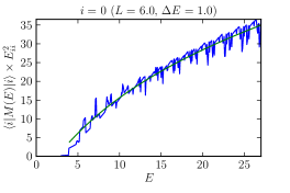
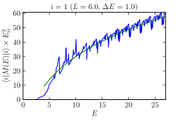
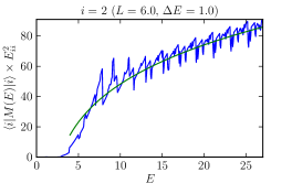
A direct check of the asymptotics (3.30) can be done by comparing it with the actual value of computed from its definition (3.13). One example is given in figure 1, where we consider the diagonal matrix elements , the state of particles at rest, . We choose , , and . The green smooth curves are the theoretical asymptotics from (3.30). The blue irregular curves represent the moving average of over the interval with . To facilitate the comparison, both are plotted multiplied by . We see that the two curves agree quite well on average.
A third test, involving the coupling, will be described in section 3.4.
3.3 Renormalization procedures
By “renormalization”, in a broad sense, we mean adding to the truncated Hamiltonian extra terms designed to compensate for the truncation effects and reduce the dependence of the results. In this section we will describe in detail the three renormalization prescriptions used in our numerical work.
Consider thus the Hamiltonian
| (3.33) |
In the main numerical studies in section 4 we will set . The opposite case , will be considered in the check in section 3.4.
We are interested in the spectrum of on a circle of length . Three approximations to this spectrum, in order of increasing accuracy, can be obtained as follows.
1. Raw truncation (marked ‘raw’ in plots)
In this simplest approach, we are not performing any renormalization. The truncated Hamiltonian is constructed by restricting to the subspace of the full Hilbert space, spanned by the states of energy . The spectrum of will be called the ‘raw spectrum’. According to Eqs. (3.30), (3.32), we expect that the raw spectrum approximates the exact spectrum with an error which scales as (up to logarithms).
2. Local renormalization (marked ‘ren.’ in plots)
In this approach, we construct a correction Hamiltonian by the formula (3.12). We use the asymptotics (3.30) for , in which we neglect with respect to . This gives a local of the form (3.11) with
| (3.34) | ||||
The choice of the reference energy will be discussed shortly. We then construct the ‘renormalized’ Hamiltonian
| (3.35) |
Thus correct the couplings, while shifts the ground state energy density. Notice that the ’s scale as (up to logarithmic terms).
The renormalized Hamlitonian acts in the same truncated Hilbert space as the truncated Hamiltonian . Its energy levels will be called the ‘renormalized spectrum’. This construction implements the first nontrivial approximation to the exact equation (3.6). The local coupling renormalization accounts for the leading error affecting the raw spectrum. Further corrections, discussed below, are suppressed by one more power of . So we expect that the renormalized spectrum approximates the exact spectrum with an error which scales as .
Let us now discuss the reference energy in (3.34). Recall that was introduced as a placeholder for the eigenstate energy in the definition (3.6) of . Now, it’s important to realize that the eigenstate energies do not remain in the limit of large . The excitations above the ground state, ,101010We use small roman letters to number states in the Fock space, which are eigenstates of , and large letters to number the eigenstates of the interacting Hamiltonian. do stay , but the ground state energy itself grows linearly:
| (3.36) |
Here is the interacting vacuum energy density (the cosmological constant), which is finite and observable in our theory.111111Recall that the free vacuum energy density was set to zero by normal ordering the free scalar Hamiltonian.
We will therefore use the following recipe. We will choose close to, although not necessarily equal, the ground state energy of the theory. The precise choice will be specified when we present the numerical results. With this choice we compute the coupling renormalizations (3.34) and the renormalized spectrum. The differences will now be , and the error induced by this mismatch will truly be suppressed. Moreover, even this error can be further corrected, as we discuss below.
We briefly mention here an alternative approach. One can insist that be adjusted, e.g. iteratively, until it exactly equals the eigenvalue which comes out from diagonalizing . This has to be done separately for each eigenstate, and so is rather expensive. We tried this method and found that it gives results in close agreement with those obtained from our simpler recipe for , combined with the correction procedure described below.
3. Local renormalization with a subleading correction (marked ‘subl.’ in plots)
We will now describe the third approach which improves on the previous one by taking into account not only the renormalization of the local couplings, but also the first subleading corrections due to the eigenstate energy and . As explained above, these corrections can be considered smaller than the local ones by a further factor. They will take care of the mismatch between (3.12) and the local coupling renormalization. The corresponding correction Hamiltonian has the following matrix elements between the truncated Hilbert space states:
| (3.37) |
(no summation over the repeated indexes). The are the differences between the renormalization coefficients fully dependent on and and the local ones defined in (3.34):
| (3.38) | ||||
There is a small technical subtlety in using the given expressions. For close to , the argument of the -functions is small in the part of the integration region close to . In this region it makes little sense to use (3.31), valid for large . From figure 1 we see that the asymptotics sets in roughly at . We therefore use the following prescription in evaluating (3.38): we use (3.31) for , while we set ’s to zero below this threshold.
The full procedure is then as follows. We compute the local renormalized Hamiltonian (3.35) with the reference value fixed around the ground state energy. We diagonalize , determining the renormalized spectrum (in practice only a few lowest eigenvalues) and the corresponding eigenstates:
| (3.39) |
Every eigenvalue is then corrected by adding (3.37) at first order in perturbation theory:
| (3.40) |
From the computational point of view the evaluation of this correction can be considered inexpensive, since it scales as the square of the basis dimension, whereas the matrix diagonalization typically scales as its cube. The energy levels will be called ‘renormalized subleading’ or simply ‘subleading’.
Second-order corrections can also be considered:
| (3.41) |
These turn out to be negligible, except when there are two almost-degenerate eigenvalues.
3.4 A test for the perturbation
We will now perform a test of our method in a controlled situation when the exact answers are known.121212This test is analogous to the one in [1], section 6. Consider the theory described by the action (cf. (2.1)):
| (3.42) |
The finite volume Hamiltonian corresponding to this problem has the form
| (3.43) |
Just as in section 2.1, the extra constant term appears because of the difference in the normal ordering counterterms in the infinite space and on the circle. These terms are exponentially suppressed for , but for the time being it will be instructive to keep them.
In full form, we have:
| (3.44) |
We expect, of course, that this Hamiltonian corresponds to a free scalar of a mass
| (3.45) |
We will now use a Bogoliubov transformation to show this explicitly. The derivation is standard and is given here only for completeness. The transformation has the form
| (3.46) |
with assumed real and depending only on . The ’s then satisfy the same oscillator commutation relations as the ’s. We want to map (3.44) onto
| (3.47) |
The conditions that the two Hamiltonians match take the form:
| (3.48) |
This is indeed satisfied provided that
| (3.49) |
which proves the expression (3.45) for the new mass. The same derivation gives the value of the vacuum energy:
| (3.50) |
Up to the constant , the last expression can be intuitively understood [1] by starting from the zero-point energy and subtracting the terms zeroth and first order in .
The series in (3.50) is convergent and can be summed using the Abel-Plana formula. We find that the constant is canceled, and the final result is given by
| (3.51) |
where is the Casimir energy of the free scalar field of mass , given by (2.10) with .
The physical interpretation of (3.51) is clear. Apart from the usual Casimir energy term, we have an induced extensive vacuum energy, corresponding to a finite vacuum energy density . Usually, when one studies the Casimir energy, the vacuum energy density in the infinite space limit is assumed to vanish. However, our situation here is different. We already finetuned to zero the vacuum energy density of the original, unperturbed, theory, i.e. the one described by the action . Once this is done, the vacuum energy density of the perturbed theory becomes finite and observable.
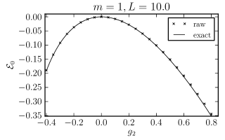
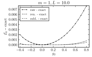
We will now compare the above exact results with the numerical results obtained by using the Hamiltonian truncation. We will be considering the case , which means that we will not be sensitive to the exponentially suppressed constant term in the initial Hamiltonian. We thus start directly from the Hamiltonian of the form (3.33) with , . We calculate its spectrum using the three procedures from section 3.3. In the shown plots we chose , , and varied from to .131313The reference energy in (3.34) was set to the value of the ground state energy given by the raw truncation procedure. For illustrative purposes numerics were done with a rather low cutoff , for which the truncated Hilbert space contains about 300 states. Figure 2 compares the ground state energy. In the left plot, the agreement between the raw and the exact result is already pretty good. The right plot shows the difference between the numerics and the exact value. We see that the renormalization greatly reduces the discrepancy over the raw procedure, and the results are made slightly better by including the subleading correction.
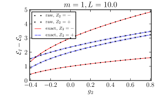
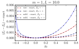
In figure 3 we do the same comparison for the spectrum of excitations above the vacuum, . In the left plot we pick the first two -odd states (one and three particles at rest), and the first two -even states (two particles at rest, and with one unit of momentum in the opposite directions). Already the raw spectrum agrees well with the exact values. In the right plot we present the differences, focussing on the first two excited levels only (one even and one odd). Notice that for the difference between and is only in the vacuum energy coefficient , which shifts all eigenvalues in the same way. The first non-trivial corrections for the spectrum of excitations are therefore the subleading ones. The improvement over the raw results is significant.
3.5 Comparison to Ref. [1]
The reader will have noticed that our treatment of the UV cutoff dependence and renormalization is similar to Ref. [1], sections 5 and 7.3. There is however a difference of principle that we will now explain.
Both in this work and in Ref. [1] the starting point for the renormalization is Eq. (3.6). While Ref. [1] also presents this equation, it then takes an alternative route, justifying the renormalization procedure on the basis of the Hamiltonian perturbation theory, see [1], Eq. (5.8). This equation is then further subjected to an RG improvement procedure in section 5.3 of [1], leading ultimately to a result which differs from our Eq. (3.6) only by some subleading corrections.
Although the RG improvement introduced in [1] might be useful for understanding the physical picture, it appears to be a detour that is not strictly necessary for doing the computations. Eq. (3.6) appears to provide the best starting point for the discussion of renormalization corrections.
A discussion on earlier approaches to analytic renormalization, in the context of TCSA, can be found section 5.4 of [1].
4 Study of the theory
In the previous sections we have developed the method and tested it in the simple setting of the perturbation. We will now move on to the main task of this paper—to study the spectrum of the theory described by the Hamiltonian (2.21).
The main physical parameter varied in our study will be the quartic coupling . The physics depends on the dimensionless ratio , and we will work in the units where the mass term .
The second parameter will be the size of the spatial circle . This plays the role of the IR cutoff, to render the spectrum discrete. In practice one is usually interested in the infinite volume limit , and we will try to approach this limit. However, even a finite is physical, in the sense that the energy levels on the circle are well-defined physical observables.
The third parameter we will vary is the cutoff on the size of the Hilbert space (the maximal energy of the free scalar Fock states included in the truncated Hilbert space). This parameter plays the role of the UV cutoff. It is unphysical. The continuum limit is recovered for .
We will typically present the results derived using the renormalization procedures both without (marked ‘ren.’ in the plots) and with (marked ‘subl.’) subleading corrections (see section 3.3). These procedures are expected to converge to the exact spectrum at the rate which goes as and (modulo logarithms). We take the difference between them as a rough idea of the current error of the method.
4.1 Varying
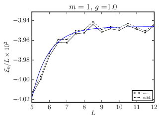
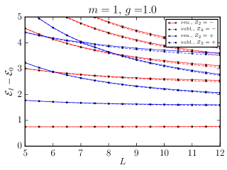
In figure 4 we present the ground state energy and the low energy spectrum of excitations for . This extends well beyond the range where perturbation theory is accurate (see appendix B). In this plot we use a fixed value , and choose the UV cutoff .141414This corresponds to keeping 12870(12801) states in the even(odd) sector of the Hilbert space. We use the two renormalization procedures explained in section 3.3.
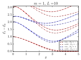
The left plot shows the dependence of the ground state ( vacuum) energy on . The vacuum is simply the state of the lowest energy, and it resides in the -even sector. There is not much structure in this plot, except for the fact that the vacuum energy is negative and grows in absolute value as is increased, becoming of the same order of magnitude as for the largest considered here. This has a consequence for the renormalization procedure used in our study. Recall that in the local renormalization (the one marked ‘ren.’) the coupling are renormalized using Eqs. (3.34) which involve the reference energy . Everywhere in this section we set to the value of the vacuum energy computed using raw truncation. We already mentioned in section 3.3 that since the vacuum energy may become large, the integrals in (3.34) have to be evaluated without expanding in . We are fortunate here that the vacuum energy becomes large and negative, and so the renormalization corrections become smaller if nonzero is taken into account. A large and positive vacuum energy would be a big problem for the performance of our method.151515That the vacuum energy becomes negative both here and in section 3.4 is probably more than just a coincidence. See the discussion in [1], note 21.
The right plot shows the 5 lowest excitations above the vacuum, with the excitations colored in blue(resp. red). As we can see the first odd level becomes almost degenerate with the vacuum for . This is a signal of the spontaneous -symmetry breaking. We therefore expect a second-order phase transition to occur at a critical point . For , the theory should flow at large distances to a CFT. Since the theory is in the same universality class as the Ising model, we expect this IR CFT to be the minimal model . We will analyze the region around in more detail below. For we are in the -broken phase. In this phase, the higher excitations should also be doubly degenerate in infinite volume. For a finite the exact degeneracy is lifted and becomes approximate. This degeneracy is not observed clearly in figure 4, probably because is not large enough.161616The discussed phase diagram is the same as for the model in dimensions studied in [1] using the TCSA. In that case it was possible to observe approximate degeneracy for the first and second excited states.
In the region of small , it is possible to validate the numerical results by comparing them to perturbation theory. In appendix B, we do this comparison for the ground state energy and the mass of the lowest excitation. For small , we find good agreement with the perturbative predictions computed through .
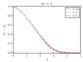
It is interesting to understand the sensitivity of the spectrum plot in figure 4 to the chosen value of . We therefore show in figure 5 similar plots for equal to , , and respectively equal to , and .171717 is adjusted to have roughly the same size of the Hilbert space in all three cases. Smaller give larger energy spacings for the one-particle momentum excitations, and allow to go to larger . To avoid clutter, only the results for the subleading renormalization (the third, most precise method in section 3.3) are presented.
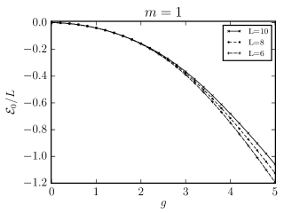
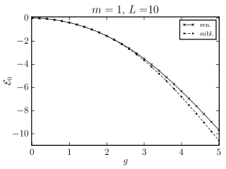
In the left plot we show the vacuum energy density . For a sufficiently large this is supposed to become independent of . We see that this constancy is verified with an excellent accuracy for . In this region we are in the massive phase, and the finite corrections are expected to be exponentially small (see section 4.3 below). The dependence on becomes more pronounced around , which is as it should be because the mass gap goes to zero here. However, in the -broken phase the corrections remain significant, while theoretically they should become again exponentially suppressed. Therefore, for , we are forced to interpret the variation with not as a physical effect but being due to finite truncation effects. This is consistent with the significant difference between the results obtained with the two renormalization procedures in figure 4.
In the right plot of figure 5 we show the physical particle mass . Once again, in the unbroken massive phase there is hardly any dependence on , while around there appears variation, which will be studied quantitatively in section 4.2 below. This plot will also be used below to extract an estimate of .
Overall, the truncation effects seem to be too large for to allow precise quantitative claims about this range of couplings (apart from the fact that the symmetry appears broken). Head-on treatment of that range would require a refinement of the method, by improving the renormalization procedure. An alternative way to access this region is to use the strong/weak coupling duality due to Chang [17]. In a companion work [18] we will both test this duality, and use it to study the -broken phase of the model.
4.2 The critical point
We will now try to determine with some precision the critical coupling , and study the lowest operator dimensions of the CFT at the phase transition. According to the standard renormalization group theory, for close to the physical mass should behave as:
| (4.1) |
where is a theory-dependent constant,181818Which also depends on from which direction one approaches the fixed point. and is a critical exponent, common for all theories in the Ising model universality class, and expressible via the dimension of the most relevant -even scalar operator, , of the CFT:
| (4.2) |
We used our numerical results obtained for , renormalized with subleading corrections (see figure 5) to perform the fit of to the formula (4.1), replacing by . Admittedly, our procedure is careless, since we do not take into account the corrections to scaling. We view the results which we will now present as preliminary; they should be validated by future studies as our method progresses. Another uncertainty concerns the range of chosen to do the fit. On the one hand, should be close to , on the other hand right close to the spectrum is modified by finite size corrections. Looking at the right plot in figure 5, we subjectively picked the -interval , which by the eye seems to give a nice powerlaw close to a straight line. To introduce some way to estimate the systematic error, we selected a few subintervals contained in the basic interval, and fitted the parameters , for each such subinterval.191919In the future, the fit procedure could be refined by taking into account the value of at . We obtained and . This value of is compatible with the two-dimensional Ising model value , giving us confidence that the procedure is sensible. To improve the estimate of , we fix to this theoretically known value and redo the fit. We then get .
The above error estimate may be too optimistic, because we completely ignored the error in induced by truncation effects. We have also performed the fit taking the , ‘renormalized subleading’ results as central values, and the difference between these central values and the ‘renormalized’ results without subleading correction as the error (we consider the two-sided error ). Following this procedure and doing the fit in the interval we obtained . This is our final, conservative, estimate.
We now perform another comparison with the theoretically known CFT operator dimensions. Namely, for the excitations should go as
| (4.3) |
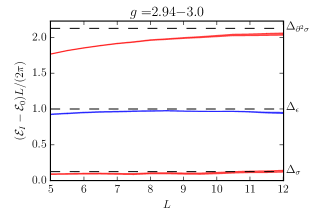
where are the CFT dimensions. This asymptotics should be valid for where the theory has flown sufficiently close to the IR fixed point. To check this, in figure 6 we plot the three lowest excitation energies multiplied by .
In this figure, we consider and vary the quartic coupling within our ‘optimistic’ uncertainty range around the fixed point, . We have to vary the UV cutoff as a function of in order to have a manageable number of basis elements in the low energy truncated Hilbert space . So decreases from at to at , while the truncated Hilbert space dimension stays for each around 10000 - 15000 per sector. To avoid clutter, we show only the ‘renormalized subleading’ results (but see figure 8 below, where the results without subleading corrections are also shown).
4.3 dependence
We will now present several plots which show explicitly how the spectrum of the theory varies for increasing while keeping fixed. These plots are analogous to figure 5, but the information is presented somewhat differently.
-unbroken phase
Let us look first at the -unbroken phase. We fix , which is at the outer border or the perturbativity range (see appendix B). Figure 7 shows then the vacuum energy density and the spectrum, for .
In the left plot we see that the vacuum energy density tends to a constant value. We don’t worry too much about the fluctuations around the limit which happen for some values of , like an upward fluctuation for or a downward fluctuation for . These fluctuations are due to the fact that in our renormalization procedure we neglected the discreteness of the distribution , replacing it by a continuous approximation. As figure 1 shows, this approximation is meant to work only on average. The sharpness of the cutoff disrupts the validity of the approximation, and must be behind the above fluctuations. In the future it will be important to find a way to work around these fluctuations. One way would be to consider a cutoff which is not totally sharp.202020Ref. [1], section 6.4 and appendix D, describes a method which for conformal bases used in that work allowed to perform renormalization taking into account the discreteness of the sequence . It’s not clear if that method extends to the massive Fock space bases used here.
Ignoring for the time being the fluctuations, let us discuss the approach of the vacuum energy density to its infinite volume limit. As is well known, in a massive phase the rate of this approach is exponentially fast and is given by:
| (4.4) |
This formula can be derived by considering the partition function of the theory on a torus where and are the lengths of the circles. The is extracted by considering the limit , and so it’s natural to treat as space and as the inverse temperature. The condition means that we are interested in low temperatures. The deviation of the free energy can then be described in terms of thermodynamics of a gas of particles of mass . This type of arguments is standard in the thermodynamic Bethe ansatz calculations in integrable theories, in which case also the subleading terms in (4.4) can be determined; see e.g. [19], Eq. (3.13). However, the leading term that we show is more general. It does not require integrability nor knowing anything about how the particles interact - we can treat them as free in this computation. In fact (4.4) can be also determined by taking the large limit of the free scalar Casimir energy (2.10) with .
The blue curve in the left plot is the fit of our numerical data by Eq. (4.4) with fixed to the value determined from the numerical spectrum (see below). We see that the rate of the approach to the infinite limit is reasonably well described by the theoretically predicted dependence.212121Since , the effect we are observing here is formally dominant with respect to the exponentially suppressed and corrections, which were omitted in section 2.1. Still, the hierarchy is not very large, and a more careful comparison may be warranted in the future, taking also those corrections into account.
The accompanying right plot shows the spectrum of excitations above the vacuum. Observe the remarkably small difference between the two renormalization procedures (we use this difference as an idea about the error of the method). The first excited state in the odd sector should for large approach the infinite-volume physical mass . It shows hardly any variation with in the shown range, which is consistent with the rate of approach being exponentially fast in [20]. We extract .
The second excited state, which belongs to the even sector, for large asymptotes to 1.47(4) which within error bars coincides with . This state corresponds to having two particles at rest. Notice that we do not observe any states in the energy range between and . Such states would be interpreted as two-particle bound states. As is well known, the interaction is perturbatively repulsive, so we do not expect bound states at weak coupling. Moreover it is known rigorously that two-particle bound states are absent everywhere below the phase transition; see [21], section 17.2. What we observe here is consistent with these results.
Notice that the ‘two-particles at rest’ state approaching , as well as the ‘three-particles at rest’ state going to , show a much larger variation with compared to the one-particle state. That this variation is not exponentially suppressed is a consequence of particle-particle interactions. Since the interactions are short-ranged, their effect is expected to go like the inverse volume, [22]. It should be possible to use this effect to extract information about the two-particle -matrix.222222Such analyses are standard in the TCSA approach to RG flows; see [23, 14] for the first and a recent example.
For small , it is easy to calculate these corrections explicitly using the first-order perturbation theory for the Hamiltonain (2.21). For the two-particle and three-particle states at rest we get232323These formulas are valid for a fixed finite and . In this limit the splittings between different states with the same number of particles are sufficiently large so that we can neglect their mixing. In the opposite limit one should apply quasi-degenerate perturbation theory.
| (4.5) |
The positiveness of the corrections explains the “bumps” at small coupling in the corresponding curves in figure 4 (the first -even and the second -odd states).
The even state just above the one asymptoting to should be identified as corresponding to two particles moving in the opposite directions on the circle with one unit of momentum each. Using the one-particle dispersion relation, the energy of this state should be roughly plus the corrections due to the particle interactions in finite volume. Because of the prefactor, the dispersion relation corrections are significant even at the maximal values of that we are considering; they seem to explain most of the difference between the first two even states. At larger , we expect the particle interaction corrections to take over, since their strength decreases only as .
Our final comment about the spectrum plot concerns the pattern of level crossings. In a non-integrable quantum field theory, we do not expect energy levels of the same symmetry to cross when varying the volume. In fact, the absence or presence of level crossings can be used as an empirical check of integrability (see [24] for a related recent discussion). Since the theory is, for all we know, non-integrable, levels with the same quantum number should not cross. Most levels in figure 7 do not cross trivially because they never come close each other. However, there is one interesting “avoided” crossing: the third and fourth levels head for a collision around but then repel. Many more such avoidances are present in the higher energy spectrum (not shown in figure 7).
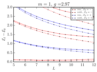
The critical point
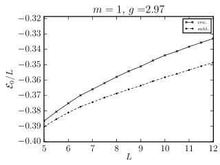
In figure 8 we show analogous plots for the neighborhood of the critical point. We fix , i.e. the central value for our estimate. One drastic change compared to figure 7 is that the energy differences (plotted on the left) no longer tend to constants but scale as , as expected for a CFT. This is the same plot as in figure 6, except that here we do not multiply by , and we show results for both renormalization methods, to get an idea of possible error bars. Evidently, even if is not exactly equal to the critical coupling, the mass gap is sufficiently small so that it is not visible for the values of shown in this plot.
On the right we show the vacuum energy density, which, as expected, seems to approach a constant. However, the uncertainty, measured by whether or not we include the subleading corrections, remains significant. Theoretically, the asymptotics of approach to the limit should be , where is the central charge of the critical point. Instead, we see something like a approach. Clearly, one should work to reduce the truncation errors before the agreement is achieved.
It should be remarked that the vacuum energy is always subject to larger errors than the spectrum of excitations. This is related to the fact that the unit operator, whose coefficient shifts the vacuum energy, is the most relevant operator of the theory, and gets the largest renormalization when the states above are integrated out. However, whichever uncertainty in the coefficient of the unit operator cancels when we compute the spectrum of excitations.
4.4 dependence
To get a better feel for the convergence of our method, and to demonstrate the difference between the three procedures explained in section 3.3, we will present here plots of the spectrum and vacuum energy as a function of , while keeping the other parameters fixed.
So, figure 9 shows the results for , , with varying from to . On the left we see that the renormalization dramatically improves the convergence of the vacuum energy with respect to the raw results, while the subsequent subleading correction is very small. The plot on the right refers to the first excited level (). In this case we see that the further improvement due to the subleading correction is non-negligible. There are small oscillations due to discretization effects, as already discussed in section 4.3. The higher excitations, not shown in the plot, show a similar pattern of convergence.
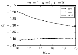
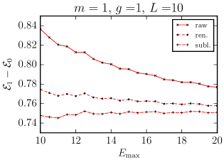
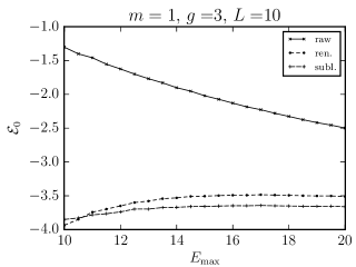
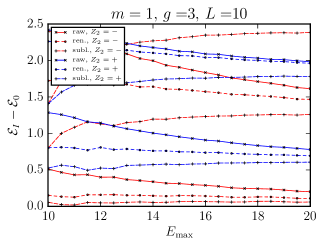
Figure 9 shows the same plots for . Once again the improvements due to renormalization are evident. For a change, here we show more states in the spectrum of excitations.
4.5 Comparison to the TCSA methods
As already mentioned, Ref. [1] recently studied the theory in dimensions using the TCSA method. The results of that study, and in particular the phase diagram of the theory, turned out to be quite similar to the one we found here; see [1], section 7. The TCSA uses the basis of conformal operators of the free massless scalar field theory, which via the state-operator correspondence is the same as the basis of states of this theory put on the sphere . In the TCSA, both the and perturbations are included into the part of the Hamiltonian. This should be contrasted with our current method, where is included into . We will mention here just one advantage and one complication of working with the conformal basis and treating all potential terms as a perturbation. The advantage is that the Hamiltonian matrix for a general sphere radius is related to the matrix via a simple rescaling. The complication is that the conformal basis is not orthonormal, requiring introduction of a Gram matrix or dealing with an eigenvalue problem which is not symmetric.
There were several reasons why [1] considered . First of all, the main point of that paper was to show that the TCSA works in . Second, there were technical reasons to postpone the physically more interesting case to the future. The final reason is that, at least naively, conformal basis does not work in , because the scalar field dimension becomes zero, rendering the spectrum dense and numerical treatment impossible.
In spite of this basic difficulty, a recent paper [4] proposed a way to use the conformal basis in dimensions. The idea of this work is to compactify the free scalar boson on a circle of a finite length . Compactification renders the CFT spectrum discrete, and one hopes that for a sufficiently small compactification effects will be negligible. It’s important to realize that the procedure of [4] modifies the quantum mechanical dynamics only for the zero mode, while all higher oscillator modes don’t feel it.242424For example, it would be wrong to think of their procedure as considering the scalar boson in a quartic potential cut off at the boundaries of the interval and periodically extended to the whole real line. Such a periodized potential would not even give a UV-complete theory, because of the spikes at the cutoff points.
On the conceptual level, the difference between our paper and [4] lies in the choice of the trial wavefunction basis for the oscillators modes. They choose periodic plane waves on a circle of radius for the zero mode, and harmonic oscillator wavefunctions of frequency for the modes with . We instead choose harmonic oscillator wavefunctions of frequency for all modes. Of course the technique for evaluating the matrix elements is also different, since we use prosaic ladder operators, while they are able to use the Kac-Moody algebra acting in the free scalar boson CFT.
Apart from which we will not discuss further, the basic parameters used in [4] to parametrize the phase diagram are: the length of the spatial circle , which is the same as our , and the quadratic and quartic couplings .252525These are denoted in [4], but we capitalized to avoid the confusion with our notation in section 3. The latter translate to our parameters as follows:262626The factor in the quartic arises from the difference of the normalization. The extra term in appears from the difference in implementing the normal ordering prescription, see their Eq. (65) and the discussion in [18].
| (4.6) | |||
| (4.7) |
In the -preserving phase, their strongest coupled point had and , which gives . From our perspective, this is an extremely weakly coupled case, where even ordinary perturbation theory would be largely adequate.
It appears that in the -preserving phase our trial wavefunction basis for the zero mode is more efficient than that of [4], since it consists of wavefunctions peaked at , as opposed to being evenly spread over a long interval. We hasten to add however that the main goal of [4] was to study the -broken phase in the regime of negative , something that we have not even attempted in this paper. In our forthcoming work [18], dedicated to the -broken phase, careful choice of the wavefunction basis for the zero mode will also play an important role.
5 Comparison with prior work
The theory in two dimensions has been previously studied, in the strongly coupled region, with a variety of techniques. Table 1 summarizes the predictions for the critical coupling. Here we only mention the methods which, at least in principle, allow for a systematic improvement of the results, leaving out simple-minded variational studies. Many of these papers normalize the quartic coupling as ; we translate all results to our normalization.
The clear trend in the table is that the critical coupling estimate seems to increase with time. The first two studies are rather old and do not assign an uncertainty to their results. The next result (DMRG) has the smallest claimed error, but as we will see below there are strong reasons to believe that it is grossly underestimated. The stated uncertainty of the two remaining predictions is also significantly smaller than ours. Their central values are below our result, although consistent with it at a level if we use the conservative error estimate. As we will discuss in section 5.4, this slight discrepancy may be due to a subtlety in implementing the matching to a continuum limit in their procedures.
| Method | Year, ref. | |
|---|---|---|
| DLCQ | 1.38 | 1988 [25] |
| QSE diagonalization | 2.5 | 2000 [5] |
| DMRG | 2.4954(4) | 2004 [26] |
| Lattice Monte Carlo | 2009 [27] | |
| Uniform matrix product states | 2.766(5) | 2013 [28] |
| Renormalized Hamiltonian truncation | 2.97(14) | This work |
We will now review the methods in Table 1, following the chronological order.
5.1 DLCQ
In [29, 25], the theory was studied using the Discretized Light Cone Quantization (DLCQ). This is a Hamiltonian truncation method in which the theory is quantized in the light-cone coordinates , using as ‘space’ and as ‘time’. The Hilbert space consists of states of several particles all moving in the direction, and having a fixed total momentum . This method was much touted in the past because of the apparent reduction in the number of states (since only particles moving in one direction are needed), and the simplicity of the vacuum structure, which in perturbation theory coincides with the free theory vacuum. In practical computations, one discretizes (hence Discretized LCQ) the momentum fraction of constituent particles with a step . This is sometimes presented as a result of compactifying the direction on a circle of length .
Refs. [29, 25] used DLCQ to compute the physical particle mass as a function of , observing that it goes to zero for a certain critical value of . They find for [29], and later report an even smaller value based on extrapolating the results to [25]. These results are in a stark disagreement with the more recent calculations by other techniques in Table 1. A careful repetition of these old studies is called for. It is known that DLCQ calculations are subject to severe truncation effects [30], which may be the source of the discrepancy.
We would like to mention here a recent proposal to avoid the discretization altogether, and instead truncate the light-cone Hilbert space by using a carefully constructed orthonormal basis of multi-particle wavefunctions. This alternative approach may be the future of the light-cone quantization. It already proved very promising in the study of 2d gauge theories [10, 11], but was not yet applied to the theory (see [12] for the preparatory work).
As a final comment on the light-cone quantization, we note that the method is bound to become more complicated in the -broken phase, possibly requiring a scan of the zero mode to find the true vacuum.
5.2 QSE diagonalization
Ref. [5] (see also [6, 7, 8]) studied the theory using the Hamiltonian truncation in the same basic setup as ours, calling it “modal field theory”. However, the implementation details are quite different. They use a quasi-sparse eigenvector (QSE) method, which reduces the Hilbert space dimension by throwing out the Fock states whose contributions to the physical eigenstate one is studying are small. In a later work [6] they developed a stochastic error correction (SEC) method, which corrects for the resulting truncation. While the idea is similar to our renormalization, there are some differences. One difference is that their method is perturbative, unlike our basic equation (3.6) which is all-order in . Another difference is that SEC computes infinite sums involved in the definition of via Monte Carlo sampling, while we found an analytic approximation for this correction term.
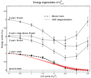
In figure 11 we show their results for the finite volume spectrum [5]. These results are based on QSE with 250 states (no SEC). Using this plot, Ref. [5] estimated the critical coupling as . On the same plot we overlay our results for the lowest -odd state from figure 4. Our predictions for the physical mass are in disagreement with [5] in the range , where the truncation errors due to finite are small. Notice that even though our results refer to a smaller value of than [5], this cannot explain the differences, since the finite volume effects for the one-particle state are negligible in this range of (see figure 7). One possible explanation is that the momentum cutoff used in [5] is not sufficiently high to describe the continuum limit. In any case, it is this disagreement which is ultimately responsible for the difference in our estimates of .
The QSE method of [6] looks somewhat similar in spirit to the Numerical RG (NRG) method recently employed in the context of TCSA [31, 24]. At the same time, the latter method seems to us more flexible and systematic. It would be interesting to apply the NRG method to the theory and see if it can help resolve the above discrepancy.
5.3 DMRG
Ref. [26] studied the theory using the Density Matrix Renormalization Group (DMRG) [32]. As a starting point of this approach, the -direction is discretized with a spacing , while time is kept continuous. The Hamiltonian describing such a discretized theory is
| (5.1) |
where are the field variables on each lattice site and are the corresponding canonical momenta. The Hilbert space on each site is infinite, unlike in the more standard DMRG applications. Ref. [26] truncates this Hilbert space to first harmonic oscillator states. The finite-system version of the DMRG algorithm [32] is used, truncating to most dominant density matrix eigenstates. This corresponds to the superblock Hamiltonian dimension .
The critical value of the coupling is obtained approaching the critical point from inside of the -broken region, and studying how the vacuum expectation value approaches zero in this limit. The quoted value has an extremely small uncertainty: . However, careful reading of the paper leaves us unconvinced that all sources of systematic error were properly taken into account. First, no attempt is made at extrapolating to , while Figure 4 of [26] shows clearly that convergence in is slow and the results for have not yet stabilized. Second, the value of is determined in Figure 7 of [26] by fitting a straight line through two points.
Finally, we believe that the matching to the continuum limit should have been done more carefully. In the units , the smallest physical lattice spacing in [26] is .272727This is found from where their smallest . This is factor 3 larger than the spacing used in the lattice Monte Carlo study [27] discussed in section 5.4 below. Since Ref. [26] used the simplest nearest-neighbor discretization of the -derivative, the matching procedure will likely be plagued by the same basic problem as the one we will explain in section 5.4.
5.4 Lattice Monte Carlo
In [27] (see [33] for earlier work) the critical coupling of the theory was determined by Monte Carlo (MC) simulations on the two-dimensional square lattice. They find , somewhat below our prediction. This discrepancy is not necessarily a reason to worry, as it may go away with further development of our method. In addition, it appears that the MC computation is subject to a subtle systematic error which was not discussed in [27]. This error is particularly troubling because similar errors likely affect, to varying degree, all techniques involving the discretization of space, including also the DMRG and MPS methods discussed in sections 5.3 and 5.5. Below we will review the lattice computation and explain this potential error.
Ref. [27] simulated the lattice action (the subscript stands for “lattice”)
| (5.2) |
Here is the lattice spacing. The normal ordering on the lattice is defined by subtracting a loop of the lattice propagator (BZ = the Brillouin zone ):
| (5.3) | |||
| (5.4) |
So operationally, (5.3) is plugged into (5.2) and the resulting action is MC-simulated.
In the normalization in which , Ref. [27] explored the range of lattice spacings - .282828See their Table II. The value of is computed from . Their lattices had up to 10241024 sites, which corresponds to a sufficiently large physical volume varying from for to for . Depending on , the critical quartic coupling was found to vary from to . Their final answer for was obtained by fitting and extrapolating to .
The systematic error that we have in mind concerns the matching between the lattice and the continuum. Naively, the lattice theory (5.2) seems to go to the continuum limit theory as , with and turning into and . However, let us try to establish this correspondence more carefully.
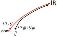
In figure 12 we show, schematically, two RG flows: the lattice flow specified by the couplings and the continuum flow specified by . The latter couplings have to be found so that the flows become the same at large distances. We can check if this is the case computing some observables at intermediate distances, when the flows are still perturbative.292929We are focussing on the case when the coupling is strong, which is relevant for the critical point. The case of small is simpler, as the matching can be performed at . If a sufficient number of observable agree at intermediate distances, the two flows have converged and will stay the same also at larger distances. In the language of effective field theory, this would be an example of perturbative matching (see e.g. [34]).303030In this discussion we ignore another complication arising from the fact that the two-dimensional theory has infinitely many additional relevant couplings beyond and , since all powers of are relevant. Strictly speaking establishing correspondence between the lattice and the continuum may require turning on these extra couplings.
At what distance scale should we do the matching? First of all, to match the continuum theory, the lattice theory should at the very least become approximately rotationally invariant. The leading deviation from rotation invariance comes from the lattice propagator (5.4), which at small momenta behaves as
| (5.5) |
To ensure that this is approximately rotationally invariant, we must have .
On the other hand, the matching momentum cannot be too small since the theory is then strongly coupled. The smallest allowed matching momentum can be computed by considering the diagrams which give a correction to the quartic coupling. For momenta these diagrams are, omitting logarithmic factors,
| (5.6) |
which becomes comparable to the coupling itself for . Putting the two constraints together, we conclude that the matching must be done at momenta such that
| (5.7) |
Now, to match the mass, we have to consider the correction to the propagator, which in the considered region of momenta behaves like
| (5.8) |
where the terms dependent on indicate the schematic dependence of the correction on the lattice spacing. This suggests that
| (5.9) |
However, such a conclusion would be on shaky grounds. The problem is that at the lowest allowed momenta the correction to the propagator due to the rotation invariance breaking has the same parametric order of magnitude, , as the putative mass matching correction.
The above discussion suggests that the chosen form of the lattice discretization prevents performing a controlled matching between the lattice and the continuum theory, because the matching corrections from loop diagrams cannot be cleanly disentangled from the rotation invariance breaking effects in the propagator. This may seem unusual to a lattice practitioner. However, the theory we are considering is a bit unusual, having a coupling constant of dimension exactly 2.
We consider it possible that this problem contributes to the mismatch between the lattice determination of and our results. Our discussion also suggests the recipe to remedy the problem: one should redo the lattice simulation using an improved actions, in which the leading effect of rotation symmetry breaking is absent due to judiciously chosen next-to-nearest interaction terms [35]. In such a setup the matching can be done, and the correspondence between and can be established rigorously.
5.5 Uniform matrix product states
This method was applied to the theory in [28]. The starting point of this approach is the discretized Hamiltonian (5.1). The lowest energy states are searched for in a finite variational subspace of the full Hilbert space, consisting of the so-called matrix product states (MPS), whose precise definition can be found in [28]. The MPS states are parametrized by a 3-tensor of size . Here, represents the size of the truncated Hilbert space per lattice site, while is a parameter which bounds the degree of entanglement of the ground state across different lattice sites. The variational states are found by minimizing the energy through an imaginary-time evolution algorithm. The physical predictions are recovered in the limit , .
As is well known, the MPS methods are essentially equivalent to DMRG (see e.g. [36]). Comparing with the DMRG study in section 5.5, and should be identified with and . Ref. [28] uses and up to 128, commenting that used in [26] are not sufficient. They observe that an insufficiently large shifts the critical point to lower , and provide a physical explanation for this effect. They do two measurements of , both approaching the critical point from above, one using and another from the lowest excitation energy. Since their two measurements differ at a level, the value cited in Table 1 was obtained by expanding the error bars to include both of them.
6 Discussion
In this work we revisited one of the simplest realizations of the “exact diagonalization” methods, as opposed to standard lattice Monte Carlo methods, and shown that it can be used effectively as a numerical tool to extract non-perturbative predictions about a quantum field theory. The numerical setup is relatively simple, and the error coming from the UV regulator can be reduced by adding analytically computed correction terms to the Hamiltonian.
Our choice of the model to study here—the two-dimensional theory—was dictated by several considerations:
-
•
the model is not supersymmetric nor integrable, hence not amenable to analytical methods, apart from perturbation theory at small coupling ;
-
•
the model has been studied in the past by a variety of numerical techniques, allowing for a fair comparison of the results and of the implementation difficulties ;
-
•
the model is literally the textbook example of a quantum field theory. In fact we hope that our exercise also has a considerable pedagogical value, helping to bridge the conceptual gap between perturbative and non-perturbative QFT questions.
However we stress that the idea of the paper is completely general, and it should be possible to apply similar techniques to any quantum field theory.
In this exploratory work we did not push particularly hard on the numerical side of the calculations—it takes a few single-core days on a desktop to reproduce all the plots in this paper. Our analytical calculations of the renormalization coefficients can and will be advanced, further improving the accuracy. The current state of the method allowed us to compute the low-energy spectrum in the -invariant phase with a reasonable accuracy, and to observe qualitatively the change to the -broken phase at strong coupling. Our estimate for the critical coupling is in a slight disagreement with the existing results. As discussed in section 5.4, this may be partly due to a technical subtlety in the lattice regularization. It would be interesting to resolve this tension in future work.
Comparisons with other Hamiltonian truncation techniques, such as TCSA or light-cone quantization, are scattered throughout the paper (see sections 3.5, 4.5, 5.1). At this point in history we don’t want to be religious about which one of these methods is most promising—all have to be explored without prejudice to see which one gives more accurate predictions, depending perhaps on the problem under consideration. One of the main challenges for all these techniques is their application to higher dimension, where the truncated Hilbert space for a given UV cutoff is larger, while the interesting interaction terms are less relevant, resulting in more significant truncation errors. In the TCSA context, these issues recently started being addressed in [1]. Another challenge is the application to gauge theories. Here the light-cone quantization seems to have gained an upper hand, at least in , thanks to the extremely efficient conformal bases recently proposed in [10, 11].
The grand question at stake is—shall we live to see the computation of the proton mass becoming accessible to every theorist, or will it forever remain in the realm of dedicated collaborations wielding supercomputers? Currently computations of the low-energy QCD spectrum with dynamical quark flavors with a few percent accuracy take about one supercomputer-year, roughly equivalent to a single-core-years.
Acknowledgements
We thank Daniele Dorigoni, Matthijs Hogervorst, Robert Konik, Giuseppe Mussardo, Agostino Patella, David Simmons-Duffin and Balt van Rees for the useful discussions, Dean Lee for the permission to use the plot in figure 11, and Mark Windoloski and Dean Lee for providing a copy of [8]. This research was partly supported by the National Centre of Competence in Research SwissMAP, funded by the Swiss National Science Foundation. The work of L.V. is supported by the Swiss National Science Foundation under grant 200020-150060.
Appendix A Speeding up the Hamiltonian matrix computation
In our computations, most time is spent in matrix diagonalization. Still, matrix evaluation should also be organized efficiently. Here we list some tricks useful to speed it up. These tricks are realized in our python code, included with the arXiv submission.
Diagonal/offdiagonal decomposition
Let’s split into three parts:
| (A.1) |
where have only diagonal/offdiagonal matrix elements. includes and the terms in of the form313131Here and below denotes an unordered set.
| (A.2) |
The rest of the terms in get assigned to and . Only the matrix elements of need to be evaluated, while those of are obtained by transposition. We include into the , terms in , as well as the operators
| (A.3) |
satisfying the following lexicographic ordering condition:323232It’s not hard to see that is impossible given and . So any operator (A.3) gets assigned either to or to .
| (A.4) |
Notice that this condition depends only on the absolute values of momenta, hence it is -invariant. This ensures that all three terms in the decomposition (A.1) are separately -invariant. This will be important below, when we describe our method to evaluate the matrix elements.
Keeping track of the energy
Each elementary operator , a product of ladder operators, increases/decreases energy of any basis vector it acts upon by a fixed amount . Since we will be working in the space of low-energy states of energies , we can drop from all operators for which
| (A.5) |
Moreover, when acting on a basis state the result is guaranteed to be zero in unless
| (A.6) |
Combinatorial factors for oscillator ordering
To reduce the number of elementary operators in , it’s worth ordering them. We have
| (A.7) |
where the symmetry factor
| (A.8) |
-conservation
In this paper we work in the Hilbert space of states of energies . Internally we represent a state , see (2.8), as a sequence of occupation numbers for each momentum mode:
| (A.9) |
where is the maximal possible mode number for the given and .
The matrix is then computed as follows. The diagonal part from is trivial so we do not discuss it. For the rest, we take a particular state and act on it with elementary operators , one by one. Each operator gives one particular state times a numerical coefficient. We accumulate this coefficient in the matrix element . Thus the matrix is generated column by column. As discussed above, we can do this computation for and get by transposition. We generate the matrix separately in each of the sectors.
The computation we just discussed produces the matrix in the full Hilbert space of , states. However, in this paper we are interested in the subspace of this space. The basis of this subspace consists of symmetrized linear combinations (2.24) of the basic Fock states. In principle, the matrix in the subspace could be obtained once the full matrix is computed, but this is wasteful. We will now describe a method which generates the matrix in the subspace directly.
When we store the symmetrized state internally, we only store . If , then we keep only one of these two vectors (no matter which one), since they give rise to the same .
We have to compute the matrix with respect to the symmerized basis, which we will call :
| (A.10) |
Consider also the matrix with respect to the Fock basis, whose computation was discussed above. Let’s split it into three pieces:
| (A.11) |
where the index runs over -invariant , and the rest of the Fock basis is split into ’s and ’s. Since , we have
| (A.12) |
and finally
| (A.13) |
From here we obtain a recipe for an economic way to compute . Namely, we compute and accumulate the coefficients and , and then multiply by .
Appendix B Perturbation theory checks
Some statements in this appendix are wrong, see Note Added below.
We computed the first two perturbative corrections to the ground state energy density and the physical particle mass for the theory defined by the action (2.1):
| (B.1) | |||
| (B.2) |
(). Recall that at is set to zero. Because the interaction is normal ordered the contributions are absent. The coefficients are numerical with a shown number of significant digits and an error estimate if needed.333333It’s likely that exact expressions for these coefficients can be found, but since this is not the focus of our work, we have not invested the effort. The size of the coefficients suggests that the series are perturbative for .
The coefficients were obtained by numerical integration of Feynman diagrams. It is much easier to perform this integration in the coordinate space, since the propagator (3.22) is exponentially decreasing at large distances, and also because parallel lines in multiloop diagrams correspond in the -space to trivially raising the propagator to a power. For example, the correction to comes from the diagram
| (B.3) |
evaluated at the (Euclidean) external momentum . In the -space this gives the integral (we omit the combinatorial factors)
| (B.4) |
We pick , introduce the polar coordinates and evaluate the integral via Monte Carlo.
In figure 13 we compare the above perturbative results with the numerical spectra obtained with our method for , . Perturbative computations refer to the infinite volume, but is sufficiently large so that the expected exponentially small corrections should not disturb the comparison. We use the cutoff . Notice that is extracted as , where is the lowest -odd eigenstate, while is extracted as .
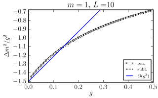
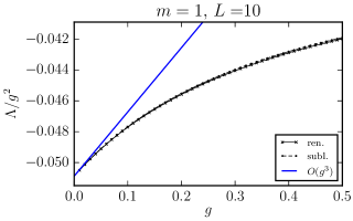
To facilitate the comparison, we plot and divided by . The reasonably good match in the region of small shows that our numerical method agrees with both and coefficients of the perturbative expansion. At the same time, higher order corrections are clearly non-negligible—they would become comparable to the correction at .
It should be noticed that it has been rigorously shown in the constructive field theory literature that perturbation theory in the two-dimensional theory is Borel-summable for small ; see [37] and the discussion in [21], section 23.2. Using Lipatov-type arguments [38, 39], the asymptotic behavior of the perturbative series coefficients is predicted to be343434The order of magnitude of coefficients (but not the alternating signs) were justified rigorously in [40].
| (B.5) |
where one has to look for a saddle point in and which gives the minimal . Given this asymptotics, one could hope that the Borel transform is regular for all positive , with a leading singularity at the negative coupling . It is not obvious to us how this analytic structure would be compatible with the phase transition at a finite .
As a side remark, we notice that the two-dimensional theory in the -symmetric phase seems sufficiently simple so that the perturbation theory can be worked out, by a numerical integration of Feynman integrals, to a very high order. The asymptotic behavior of the coefficients can be also worked out with many subleading terms. Given that, we would like to challenge the resurgence/Borel transform community (see e.g. [41]) to reproduce the dependence with a precision matching that of our method.
Note added (Aug 2018) The coefficient in (B.2) is wrong as we forgot to include another diagram which contributes this coefficient. With both diagrams included, the value of the coefficient changes to . Analytic values of both diagrams were computed in [42] which reacted to the challenge stated in the previous paragraph. With the coefficient corrected, the perturbative prediction becomes tangent to the numerical one at small ; see Fig. 14. We thank Marco Serone, Gabriele Spada and Giovanni Villadoro for their magnificent paper, and for informing us about our mistake.
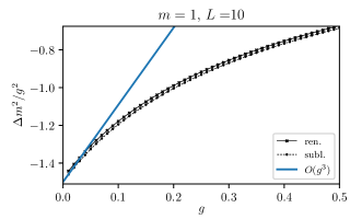
References
- [1] M. Hogervorst, S. Rychkov, and B. C. van Rees, “Truncated conformal space approach in dimensions: A cheap alternative to lattice field theory?,” Phys. Rev. D91 (2015) 025005, arXiv:1409.1581 [hep-th].
- [2] S. J. Brodsky, H.-C. Pauli, and S. S. Pinsky, “Quantum chromodynamics and other field theories on the light cone,” Phys.Rept. 301 (1998) 299–486, arXiv:hep-ph/9705477 [hep-ph].
- [3] V. P. Yurov and Al. B. Zamolodchikov, “Truncated Conformal Space Approach to Scaling Lee-Yang Model,” Int.J.Mod.Phys. A5 (1990) 3221–3246.
- [4] A. Coser, M. Beria, G. P. Brandino, R. M. Konik, and G. Mussardo, “Truncated Conformal Space Approach for 2D Landau-Ginzburg Theories,” J. Stat. Mech. 1412 (2014) P12010, arXiv:1409.1494 [hep-th].
- [5] D. Lee, N. Salwen, and D. Lee, “The Diagonalization of quantum field Hamiltonians,” Phys.Lett. B503 (2001) 223–235, arXiv:hep-th/0002251 [hep-th].
- [6] D. Lee, N. Salwen, and M. Windoloski, “Introduction to stochastic error correction methods,” Phys.Lett. B502 (2001) 329–337, arXiv:hep-lat/0010039 [hep-lat].
- [7] N. Salwen, Non-perturbative methods in modal field theory. arXiv:hep-lat/0212035 [hep-lat]. Ph.D. thesis, Harvard University, 2001.
- [8] M. Windoloski, A Non-perturbative Study of Three-Dimensional Quartic Scalar Field Theory Using Modal Field Theory. Ph.D. thesis, University of Massachusetts Amherst, 2000.
- [9] I. Brooks, E.D. and S. C. Frautschi, “Scalars Coupled to Fermions in (1+1)-dimensions,” Z.Phys. C23 (1984) 263.
- [10] E. Katz, G. M. Tavares, and Y. Xu, “Solving 2D QCD with an adjoint fermion analytically,” JHEP 1405 (2014) 143, arXiv:1308.4980 [hep-th].
- [11] E. Katz, G. M. Tavares, and Y. Xu, “A solution of 2D QCD at Finite using a conformal basis,” arXiv:1405.6727 [hep-th].
- [12] S. Chabysheva and J. Hiller, “Basis of symmetric polynomials for many-boson light-front wave functions,” arXiv:1409.6333 [hep-ph].
- [13] P. Giokas and G. Watts, “The renormalisation group for the truncated conformal space approach on the cylinder,” arXiv:1106.2448 [hep-th].
- [14] M. Lencses and G. Takacs, “Excited state TBA and renormalized TCSA in the scaling Potts model,” JHEP 09 (2014) 052, arXiv:1405.3157 [hep-th].
- [15] S. R. Coleman, “The Quantum Sine-Gordon Equation as the Massive Thirring Model,” Phys.Rev. D11 (1975) 2088.
- [16] M. Bordag, G. L. Klimchitskaya, U. Mohideen, and V. M. Mostepanenko, “Advances in the Casimir effect,” Int. Ser. Monogr. Phys. 145 (2009) 1–768.
- [17] S.-J. Chang, “The Existence of a Second Order Phase Transition in the Two-Dimensional Field Theory,” Phys.Rev. D13 (1976) 2778.
- [18] S. Rychkov and L. G. Vitale, “Hamiltonian truncation study of the theory in two dimensions. II. The -broken phase and the Chang duality,” Phys. Rev. D93 no. 6, (2016) 065014, arXiv:1512.00493 [hep-th].
- [19] A. Zamolodchikov, “Thermodynamic Bethe Ansatz in Relativistic Models. Scaling Three State Potts and Lee-Yang Models,” Nucl.Phys. B342 (1990) 695–720.
- [20] M. Lüscher, “Volume Dependence of the Energy Spectrum in Massive Quantum Field Theories. 1. Stable Particle States,” Commun.Math.Phys. 104 (1986) 177.
- [21] J. Glimm and A. M. Jaffe, Quantum Physics. A Functional Integral Point Of View. Springer, 1987.
- [22] M. Lüscher, “Volume Dependence of the Energy Spectrum in Massive Quantum Field Theories. 2. Scattering States,” Commun.Math.Phys. 105 (1986) 153–188.
- [23] V. Yurov and Al. B. Zamolodchikov, “Truncated fermionic space approach to the critical 2-D Ising model with magnetic field,” Int.J.Mod.Phys. A6 (1991) 4557–4578.
- [24] G. Brandino, R. Konik, and G. Mussardo, “Energy Level Distribution of Perturbed Conformal Field Theories,” J.Stat.Mech. 1007 (2010) P07013, arXiv:1004.4844 [cond-mat.stat-mech].
- [25] A. Harindranath and J. Vary, “Stability of the Vacuum in Scalar Field Models in 1 + 1 Dimensions,” Phys.Rev. D37 (1988) 1076–1078.
- [26] T. Sugihara, “Density matrix renormalization group in a two-dimensional lambda Hamiltonian lattice model,” JHEP 0405 (2004) 007, arXiv:hep-lat/0403008 [hep-lat].
- [27] D. Schaich and W. Loinaz, “An improved lattice measurement of the critical coupling in theory,” Phys.Rev. D79 (2009) 056008, arXiv:0902.0045 [hep-lat].
- [28] A. Milsted, J. Haegeman, and T. J. Osborne, “Matrix product states and variational methods applied to critical quantum field theory,” Phys.Rev. D88 (2013) 085030, arXiv:1302.5582 [hep-lat].
- [29] A. Harindranath and J. Vary, “Solving Two-Dimensional Theory By Discretized Light Front Quantization,” Phys.Rev. D36 (1987) 1141–1147.
- [30] B. van de Sande, “Convergence of discretized light cone quantization in the small mass limit,” Phys.Rev. D54 (1996) 6347–6350, arXiv:hep-ph/9605409 [hep-ph].
- [31] R. M. Konik and Y. Adamov, “Numerical renormalization group for continuum one-dimensional systems,” Phys. Rev. Lett. 98 (2007) 147205, arXiv:cond-mat/0701605 [cond-mat.str-el].
- [32] S. R. White, “Density-matrix algorithms for quantum renormalization groups,” Phys. Rev. B 48 (1993) 10345.
- [33] W. Loinaz and R. Willey, “Monte Carlo simulation calculation of critical coupling constant for continuum in two-dimensions,” Phys.Rev. D58 (1998) 076003, arXiv:hep-lat/9712008 [hep-lat].
- [34] I. Z. Rothstein, “TASI lectures on effective field theories,” arXiv:hep-ph/0308266 [hep-ph].
- [35] K. Symanzik, “Continuum Limit and Improved Action in Lattice Theories. 1. Principles and Theory,” Nucl.Phys. B226 (1983) 187.
- [36] U. Schollwöck, “The density-matrix renormalization group in the age of matrix product states,” Annals of Physics 326 (2011) 96.
- [37] J.-P. Eckmann, J. Magnen, and R. Sénéor, “Decay properties and Borel summability for the Schwinger functions in theories,” Comm. Math. Phys. 39 (1975) 251.
- [38] L. Lipatov, “Divergence of Perturbation Series and Pseudoparticles,” JETP Lett. 25 (1977) 104–107.
- [39] E. Brezin, J. Le Guillou, and J. Zinn-Justin, “Perturbation Theory at Large Order. 1. The Interaction,” Phys.Rev. D15 (1977) 1544–1557.
- [40] S. Breen, “Leading Large Order Asymptotics For Perturbation Theory,” Commun.Math.Phys. 92 (1983) 179–194.
- [41] A. Cherman, D. Dorigoni, G. V. Dunne, and M. Ünsal, “Resurgence in Quantum Field Theory: Nonperturbative Effects in the Principal Chiral Model,” Phys.Rev.Lett. 112 no. 2, (2014) 021601, arXiv:1308.0127 [hep-th].
- [42] M. Serone, G. Spada, and G. Villadoro, “ Theory I: The Symmetric Phase Beyond NNNNNNNNLO,” arXiv:1805.05882 [hep-th].