Causal Dynamical Triangulations (CDT) provide a non-perturbative formulation of Quantum Gravity assuming the existence of a global time foliation. In our earlier study we analyzed the effect of including $d$ copies of a massless scalar field in the two-dimensional CDT model with imaginary time. For $d>1$ we observed the formation of a “blob”, somewhat similar to that observed in four-dimensional CDT without matter. In the two-dimensional case the “blob” has a Hausdorff dimension $D_{H}=3$. In this paper we study the spectral dimension $D_{S}$ of the two-dimensional CDT-universe, both for $d=0$ (pure gravity) and $d=4$. We show that in both cases the spectral dimension is consistent with $D_{S}=2$.

1 Introduction

Quantizing gravity remains one of big challenges for Theoretical Physics. Causal Dynamical Triangulations (CDT) is one of a number of attempts to define non-perturbatively a theory of quantum gravity. We refer to [1] for a recent review. In CDT spacetime is discretized (triangulated) in such a way that a global time foliation exists. This time foliation permits one to perform a Wick rotation to imaginary time for each configuration, and it makes it possible to study the CDT spacetimes using standard methods of statistical mechanics, i.e. Monte Carlo simulations.

The existence of a global time foliation has important consequences. The regularized theory of quantum gravity defined this way differs from the regularized theory without this constraint. If the constraint of a time foliation is not imposed and we use triangulations with Euclidean signature, the regularization is denoted Euclidean dynamical triangulation (EDT). In four dimensions EDT seems not to result in an interesting continuum limit when the UV cut off (the link length in the triangulations) is taken to zero. That was the reason for inventing the formalism of CDT, which might indeed have an interesting continuum limit in the case of the three– and four–dimensional theories, [2, 3, 4, 5]. The regularized two-dimensional theories can be solved analytically both for CDT and for EDT [6, 7, 8] and the continuum limit corresponds to 2d Hořava-Lifshitz quantum gravity [12, 13] and $c_{L}=26$ Liouville quantum gravity [9, 10, 11], respectively, ($c_{L}$ denoting the central charge of the Liouville theory). If one couples matter to the regularized 2d quantum gravity theories one can explicitly solve modified EDT models which in the continuum limit correspond to rational (p,q)-minimal conformal field theories with central charge $c_{M}\leq 1$ coupled to 2d Liouville quantum gravity with corresponding Liouville central charge $c_{L}=26-c_{M}$. When $c_{M}>1$ the combined regularized theory seeming degenerate to a theory of branched polymers. This is the so-called $c_{M}=1$ barrier. It has not been possible to solve analytically CDT coupled to matter fields except in a few cases where the relation to a central charge of the matter fields is not so clear [14]. However, one can study CDT coupled to matter fields with well-defined central charges numerically. Ising models and Potts models coupled to CDT, as well as Gaussian scalar fields coupled to CDT have been studied using Monte Carlo simulations [15, 16].

In these Monte Carlo simulations the following was observed: for $c_{M}\leq 1$ the interaction between matter and geometry is weak in the sense that the critical exponents of the matter fields are the same as the exponents of matter fields in flat spacetime (this is in contrast to the critical exponents of matter in EDT). At the same time the Hausdorff dimension $d_{H}$ of the CDT spacetime is 2 if the matter fields have central charges $0\leq c_{M}\leq 1$ (again in contrast to the Hausdorff dimension of EDT spacetime). However, like in EDT there seems to be a $c_{M}=1$ barrier. The EDT $c_{M}=1$ barrier can be viewed as the proliferation of baby universes such that the EDT geometries degenerate into so-called branched polymers. The imposed time foliation in CDT prevents such a generation of baby universes. Instead the $c_{M}=1$ barrier manifests itself by the generation of a “blob”. By a “blob” we mean the following: in the computer simulations we choose a certain volume of spacetime, i.e. the number of triangles $N$. Also we choose a certain number of time-foliations $L$. For each lattice time $t\in[0,L]$ there is associated a space-volume $n(t)$. However, for a fixed $N$ and if $L$ is sufficiently large, the space volume $n(t)$ is only significantly different from zero in some sub-interval of $L$. This defines the extent of the blob, and this distribution of $n(t)$ is in sharp contrast with the situation for $c_{M}\leq 1$ where $n(t)$ is uniformly distributed over the whole range $L$ of times. Moreover the time extension of the blob seems to scale universally as $N^{1/3}$ no matter which $c_{M}>1$ is used and which kind of critical matter (Gaussian fields, multiple Ising spins etc.) one uses. This scaling behavior indicated that the Hausdorff dimension $D_{H}$ of the blob is 3. The formation of a “blob” has been observed also in higher dimensional CDT where it has been identified with a “de Sitter” like phase of the quantum universe of the CDT model [17, 4].

To further understand the geometries generated by the CDT models, we measure in this article the spectral dimension $D_{S}$ of two-dimension CDT, both for $c_{M}=0$ and for $c_{M}>1$ where we have the dynamical generation of a “blob”. We use the diffusion equation on the CDT configurations to determine the spectral dimension and we find $D_{S}=2$ in all cases. The topology of the spacetime manifold we use is by construction that of a torus. However, as described above, when a blob is formed we have effectively a change in topology from a torus to a sphere since the thin “stalk” which constitutes spacetime outside the blob carries almost no spacetime volume. We show that the standard method used to measure $D_{S}$ can be used to discriminate between the two if we use suitable long diffusion time.

In Sec.  2 we briefly recall the definition of the 2d CDT model and the geometric scaling used in the case of pure gravity and gravity interacting with matter fields. In the Sec.  3 we shortly discuss the behavior of the spectral dimension defined using the return probability of the diffusion process on a regular two-dimensional surface with a topology of a torus and of a sphere. We use these results to analyze results of numerical simulations in the cases $c_{M}=0$ and $c_{M}=4$ (four Gaussian fields coupled to geometry). The last section contains conclusions and discussion.

2 Definition of the 2d CDT model

The CDT model in 1+1 dimensions represents the path integral as a sum over piecewise linear spacetimes built of triangles [6]. The vertices of triangles are parametrized by an integer time variable, with two vertices at time $t$ and one vertex at $t\pm 1$. Spatial slices at integer time have the topology of the circle $S_{1}$. An alternative formulation can be based on the dual lattice with points in the centers of the triangles, connected by links, dual to the links of the original triangles. The dual vertices can be viewed as placed at half-integer times. In the dual formulation each vertex is connected to three other vertices, two in the same time slice and one above or below at half-integer time. Links joining vertices with the same time index form a circle. The dual formulation is completely equivalent to the one formulated in terms of triangles and will be used in this paper. In [6] the starting point was Lorentzian spacetime, where two of the links of each triangle had time-like signature. However, a Wick rotation could be performed for each triangulation such that all triangles became ordinary Euclidean equilateral triangles where all links have lengths $a$. We work here with this Wick rotated CDT version. In practice we take $a=1$ and postpone the discussion of the continuum limit $a\to 0$ until later. In this formulation we map the quantum system into a statistical system, described by the partition function

$$Z=\sum_{T}\int^{\prime}\prod_{i,\mu}d\phi_{i}^{\mu}\;\frac{1}{C_{T}}\;\exp\left(-\lambda N_{T}-S_{M}(\phi_{i}^{\mu})\right)$$ (1)

where $\lambda$ is a cosmological constant, $N_{T}$ is the number of vertices in a (dual) triangulation $T$ and $C_{T}$ is a symmetry factor of the triangulation. $S_{M}(\phi)$ denotes the matter action coupled to geometry. We choose here $d$ Gaussian scalar fields $\phi_{i}^{\mu},~{}\mu=1,\dots,d$, which thus represent a conformal field theory with central charge $c_{M}=d$. The discretized Gaussian action, suitable for the (dual) triangulation is

$$S_{M}=\frac{1}{2}\sum_{i\leftrightarrow j,\mu}(\phi_{i}^{\mu}-\phi_{j}^{\mu})^{2}$$ (2)

The summation is over all neighboring pairs of vertices. The action is invariant under translation $\phi_{i}\to\phi_{i}+\phi_{0}$, and we fix this zero-mode in the action (2) by fixing the ”center of mass” of $\phi$. This is indicated by the prime-label in $\int$. $d=0$ corresponds to pure CDT gravity where $c_{M}=0$. The requirement that the universe (the dual triangulation) does not consist of disconnected components implies that at each time slice of the dual lattice we have at least one link pointing back in time and one link pointing forward. For convenience of the computer simulations and in order to minimize boundary effects we choose periodic boundary conditions in the time directions and we fix the number of integer time steps to be $L$. The partition function (1) can be expressed as a sum

$$Z=\sum_{N}e^{-\lambda N}\;Z_{N},$$ (3)

where in $Z_{N}$ we sum over triangulations with $N$ vertices. A simple quantity we can measure in the computer simulations is the spatial volume distribution as a function of time: $n(t)$. For two-dimensional spacetime $n(t)$ will be a length, and in our (dual) triangulation it will be the number of vertices at time $t$. If a given triangulation has $N$ vertices we obviously have $\sum_{t}n(t)=N$. As mention above it is precisely $n(t)$ which signals the $c_{M}=1$ transition ($n(t)$ changes from an uniform distribution to a “blob”-distribution).

For the model containing scalar matter fields an analytic solution is not known but the model can readily be studied using numerical methods. When performing Monte Carlo simulations it is convenient to (approximately) fix the spacetime volume $N$ (the number of vertices). In order to do that we use a modified partition function

$$Z_{N}=\sum_{N_{T}}\exp\left(-\lambda N_{T}\right)Z_{N_{T}}\exp\left(-\frac{\epsilon}{2}(N_{T}-N)^{2}\right)$$ (4)

where $\epsilon$ controls the size of spacetime volume fluctuations. This technique was used successfully in [16] where models with $d\geq 1$ were studied. What we observed by measuring $n(t)$ using the partition function (4) was the formation of a “blob” for $d>1$, very similar to what happens in higher dimensional CDT, as mentioned above. Fig.  1 presents such blob-profiles $n_{N}(t)$ for the case of four Gaussian fields ($d=4$). The left figure shows the average spatial volume profile $n_{N}(t)$ for different values of the spacetime volume $N$. The right figure shows that all these curves can be scaled to form a universal curve $n_{U}(t_{U})=N^{1-1/D_{H}}n_{N}(t/N^{1/D_{H}})$ with $D_{H}=3$ being the the Hausdorff dimension of the blob.

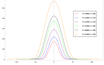
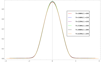
Figure 1: Average volume profile for $d=4$ (left). Universal scaled profile, assuming Hausdorff dimension $D_{H}=3$ (right).

The behavior shows that matter plays a very important role, inducing a quite nontrivial scaling of the geometry even for this simple model. When $N\to\infty$ the “stalk”, the spacetime outside the blob, effectively disappears and it is only present because our computer algorithm does not allow the spatial volume at a given time to be zero. The creation of a “blob” with non-trivial scaling properties and a corresponding stalk should be compared to the situation where $c_{M}\leq 1$. In Fig. 2 we present similar measurements for the case $d=0$. The $n(t)$’s on the plot have an artificial maximum around time $t=0$, because our procedure of superimposing different measured configurations defines a “center of mass” and allocates time $t=0$ to this center of mass before making the superposition. In this way we explicitly break the time-translation invariance. One observes that no stalk (and thus no blob) is formed. As before the spatial volume profiles $n_{N}(t)$ can be scaled to a universal profile $n_{U}(t_{U})$, but this time with the canonical dimension $D_{H}=2$ which one would naively expect.

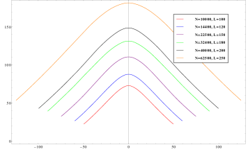
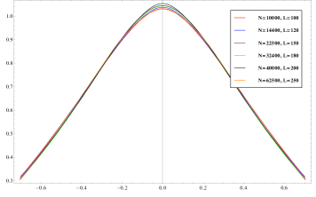
Figure 2: Average volume profile for pure gravity (left) and it’s scaled version (right).

3 The spectral dimension

On a fixed, smooth geometry the diffusion process is governed by the diffusion equation

$$\frac{\partial}{\partial\sigma}\,K_{g}(\xi,\xi_{0};\sigma)=\Delta_{g}K_{g}(\xi,\xi_{0};\sigma),$$ (5)

where $\sigma$ is the fictitious diffusion time and $\Delta_{g}$ the Laplace operator corresponding to the metric $g_{ab}(\xi)$. $K_{g}(\xi,\xi_{0};\sigma)$ is the probability density of diffusion from $\xi_{0}$ to $\xi$ in a diffusion time $\sigma$. The return probability is defined as $K(\xi_{0},\sigma)=K_{g}(\xi=\xi_{0};\sigma)$ and one has the following behavior for short diffusion time $\sigma$:

$$K(\xi_{0},\sigma)\sim\frac{1}{\sigma^{D_{S}/2}}(1+O(\sigma)),~{}~{}~{}D_{S}=-2\lim_{\sigma\to 0}\log K(\xi_{0},\sigma).$$ (6)

where $D_{S}$ is denoted the spectral dimension and for a smooth manifold is equal to the dimension $D$ of the manifold. The correction $O(\sigma)$ has an asymptotic power expansion in $\sigma$ (the heat kernel expansion) where the coefficients depend on the local curvature and derivatives of the curvature at $\xi_{0}$.

Let us consider the return probability in two cases: a two-dimensional sphere with the radius $R$ and a two-dimensional torus with the radii $R_{1}$ and $R_{2}$ with $R_{1}R_{2}=R^{2}$ and $R_{1}/R_{2}=\rho$. In both cases the $K(\xi_{0},\sigma)$ does not depend on the initial position $\xi_{0}$ and we write $K_{g}(\xi=\xi_{0};\sigma)=K(\sigma)$. For the sphere we have

$$K(\sigma)\propto\sum_{n=0}^{\infty}(2n+1)e^{-n(n+1)\sigma/R^{2}},$$ (7)

while the expression for the torus is

$$K(\sigma)\propto(1+2\sum_{p=1}^{\infty}e^{-\frac{4p^{2}\pi^{2}\sigma}{R^{2}\rho}})(1+2\sum_{q=1}^{\infty}e^{-\frac{4q^{2}\pi^{2}\sigma\rho}{R^{2}}}).$$ (8)

In both cases we define

$$D_{S}(\sigma)=-2\frac{d\log K(\sigma)}{d\log\sigma},~{}~{}~{}{\rm i.e.}~{}~{}~{}\lim_{\sigma\to 0}D_{S}(\sigma)=D_{S}.$$ (9)

In Fig. 3 we show the behavior of $D_{S}(\sigma)$ for small $\sigma$. In both cases $D_{S}(\sigma)=2$ for small $\sigma$ since the spacetime is two-dimensional. Further, in both cases $D_{S}(\sigma)$ eventually goes to zero simply because we have a finite spacetime volume and the large time diffusion will be dominated by the zero mode of the Laplacian, the constant mode, i.e. $K(\xi,\xi_{0},\sigma)\propto 1/V$ for $\sigma\to\infty$. For a torus we see a non-trivial dependence on $\rho$.

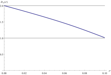
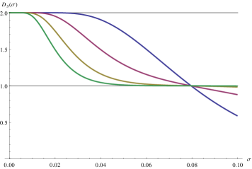
Figure 3: Behavior of $D_{S}(\sigma)$ for a sphere (left) and for a torus (right). In all cases the area of a manifold is $1$. For a torus we show curves for $\rho=1,2,3,4$ and $R^{2}=1$.

This dependence is illustrated in Fig. 4. For $R_{2}>>R_{1}$ we see the appearance of a second plateau at $D_{S}\approx 1$, reflecting the effective one-dimensional structure at a larger scale. Thus $D_{S}(\sigma)$ contains information about the spectral dimension ($D_{S}=2$ in both cases due to the small $\sigma$ behavior) and about the large scale geometry of the manifold (obtained for intermediate $\sigma$). Finally, the scaling for intermediate and large $\sigma$ also provides information about $D_{S}$ since one in this region can obtain scaling by using the variable $\sigma/V^{2/D_{S}}$ and comparing the diffusion for different spacetime volumes $V$.

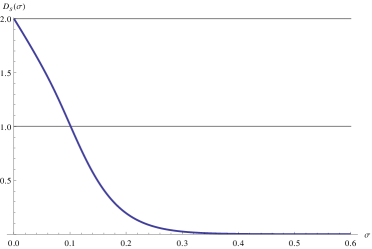
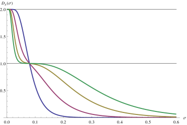
Figure 4: $D_{S}(\sigma)$ for a sphere (left) and a torus (right) for large $\sigma$. In the right plot we compare the behavior for a torus with $\rho=1,~{}2,~{}3$ and 4.

The matter action used in (2) leads to a natural discretized version of the scalar Laplacian which appears in eq. (5). The spectral properties of this operator can be analyzed in order to obtain additional information about the fractal properties of the “blob”-geometry. The diffusion process in the discrete diffusion-time variable $s$ defines a probability field $P_{i}(s;T)$ for a particular geometric configuration $T$ ($i$’s label vertices in the triangulation $T$) by the following equation, which is the discrete analogy of the standard diffusion equation (5):

$$P_{i}(s+1;T)=\frac{1}{3}\sum_{j\to i}P_{j}(s;T)$$ (10)

The summation is over the three vertices $j$ neighboring vertex $i$. The initial condition for $s=0$ is $P_{i}(0;T)=\delta_{i,i_{0}}$, where typically $i_{0}$ is chosen to belong to spatial slice with the largest spatial volume. We measure the average return probability $P(s)=\langle P_{i_{0},i_{0}}(s;T)\rangle$ where the average is taken over initial points $i_{0}$ and configurations $T$. The diffusion process is performed on systems with a finite spacetime volume $N$ and again we study the limiting behavior and the scaling for large $N$. A function $D_{S}(s)$ which is the discretized analogy to (6) is defined as

$$D_{S}(s+1)=-2\log\left(\frac{P(s+2)}{P(s)}\right)/\log\left(\frac{s+2}{s}\right).$$ (11)

We use the discretized logarithmic derivative in the expression above in a form which permits to discriminate between even and odd times $s$.

Below we show that we have qualitatively similar behavior to $D_{S}(\sigma)$ when we measured (11) for CDT triangulations. Extracting information from such numerical “measurements” requires some care. We would like to define the spectral dimension $D_{S}$ as the limit of the function $D_{S}(s)$ for small $s$. However, for very short time $s=1,2,\ldots,s_{0}$ we expect lattice artifacts to interfere with the “correct” continuum result (below we will see that $s_{0}\approx 200$). For larger times the value of $D_{S}$ is seen as a plateau of the function $D_{S}(s)$, but there will be an uncertainty in identifying the plateau and extracting the corresponding value $D_{S}$. For even larger times we expect scaling similar to that described for smooth 2d manifolds as a function of the spacetime volume $N$, but for sufficient long diffusion times we enter a range where we may have a combination of numerical uncertainty and finite-size effects related to the stalk/bulk interference (in the case where we have a “blob”).

Let us first discuss the case $d=4$. In Fig. 5 we show the dependence of $D_{s}(s)$ for small $s$ and we compare it with the pure gravity ($d=0$) behavior. In both cases the plot of $D_{s}(s)$ splits for very small $s$ into two curves, corresponding to even and odd diffusion times. This is a typical lattice artifact. We can trust the estimate only for times larger than the range of the even/odd split at $s\approx 200$. For larger $s$ the plot has a plateau corresponding to $D_{S}\approx 2$, similar to that for a continuous two-dimensional geometry.

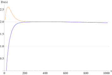
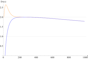
Figure 5: Dependence of $D_{s}(s)$ for $d=4$ (left) and pure gravity (right) at small $s$, $N=40000$, $L=200$ for both cases.

We conclude that the value of the spectral dimension is consistent with the canonical value $D_{S}=2$ both for $d=4$ and $d=0$. For $d=0$ this was expected since we have in that case $D_{H}=2$ and since all indication is that for $c_{M}\leq 1$ the CDT geometries can be considered as genuine two-dimensional without any significant fractal structure.

For $d=4$ it was not clear what to expect. As mentioned above the Hausdorff dimension is in this case $D_{H}=3$. The value $D_{H}=3$ is thus not transmitted to the spectral dimension $D_{S}$. The value $D_{S}=2$ is further confirmed by looking at the scale dependence of $D_{S}(s)$. In Fig.  6 we plot $D_{S}(s)$ as a function of the scaling variable $s/N^{2/D_{S}}$ with $D_{S}=2$. For the range of $s$ studied we see no trace of the toroidal geometry. Diffusion is completely dominated by the “blob”.

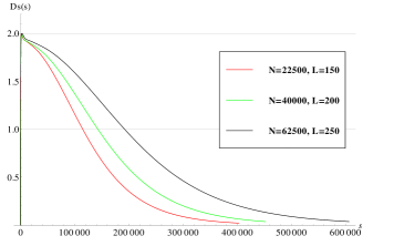
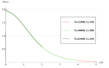
Figure 6: Scaling of $D_{S}(s)$ as a function of $s$ for $d=4$ and a number of volumes $N$. The left plot is not scaled, the right plot is the same curve scaled as a function of $s/N$.

This is in contrast to the case of pure gravity ($d=0$). In Fig. 7 we show $D_{S}(s)$ measured for $d=0$. It behaves qualitatively similar to $D_{S}(s)$ calculated using the continuum diffusion equation on a regular torus and it shows scaling when we use the re-scaled diffusion time $s/N$. The plateau $D_{S}(s)=1$ as a function of $\rho$ is shown in Fig.  8. We see as expected that the plateau becomes more pronounced with increasing $\rho$.

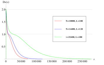
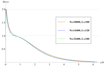
Figure 7: Scaling of $D_{S}(s)$ as a function of $s$ for pure gravity and a number of volumes $N$. The left plot is not scaled, the right plot is the same curve scaled as a function of $s/N$.

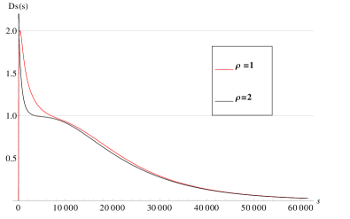
Figure 8: $D_{S}(s)$ for pure gravity: $\rho=1$ and $\rho=4$, we set $N=10000$ for both cases and $L=100$ and $L=200$.

4 Summary

We have measured the spectral dimension of two-dimensional CDT quantum gravity coupled to four scalar fields. In this model spacetime scales anomalously, forming a blob where the time scales as $N^{1/3}$ and space as $N^{2/3}$, $N$ being the volume of spacetime. We found that despite of this anomalous scaling, indicating that the Hausdorff dimension $D_{H}=3$, the spectral dimension $D_{S}=2$, like for smooth two-dimensional spacetimes.

We compared this behavior with that of pure gravity (two-dimensional CDT without matter fields), where the Hausdorff dimension $D_{H}=2$ and where no blob is formed. Although this system admits the existence of an analytic solution for some quantities of interest, this is not the case for the heat kernel of the Laplacian, which has to be studied numerically. We show that the spectral dimension is $D_{S}=2$, but in contrast to the $d=4$ case the diffusion would explore the full toroidal topology, and by varying the asymmetry parameter $\rho$ of the torus one could observe a secondary plateau at $D_{S}=1$, expressing the fact if one of the radii of the torus is small, long time diffusion will effectively see a one-dimensional thin tube.

Acknowledgments. HZ is partly supported by the International PhD Projects Programme of the Foundation for Polish Science within the European Regional Development Fund of the European Union, agreement no. MPD/2009/6. JJ acknowledges the support of grant DEC-2012/06/A/ST2/00389 from the National Science Centre Poland. JA and AG acknowledge support from the ERC-Advance grant 291092, “Exploring the Quantum Universe” (EQU). JA acknowledges support of FNU, the Free Danish Research Council, from the grant “quantum gravity and the role of black holes”.

References

- [1] J. Ambjørn, A. Görlich, J. Jurkiewicz and R. Loll, Phys. Rept. 519 (2012) 127 [arXiv:1203.3591, hep-th].
-
[2]
J. Ambjorn, J. Jurkiewicz and R. Loll,
Phys. Rev. D 64 (2001) 044011
[hep-th/0011276].
C. Anderson, S.J. Carlip, J.H. Cooperman, P. Hořava, R.K. Kommu and P.R. Zulkowski, Phys. Rev. D 85 (2012) 044027 [arXiv:1111.6634, hep-th].
S. Jordan and R. Loll, Phys. Lett. B 724 (2013) 155-159 [arXiv:1305.4582, hep-th]; Phys. Rev. D 88 (2013) 044055 [arXiv:1307.5469, hep-th]. - [3] J. Ambjørn, J. Jurkiewicz and R. Loll, Nucl. Phys. B 610 (2001) 347 [hep-th/0105267]; Phys. Rev. D 72 (2005) 064014 [hep-th/0505154]; Phys. Rev. Lett. 93 (2004) 131301 [hep-th/0404156].
- [4] J. Ambjørn, A. Görlich, J. Jurkiewicz and R. Loll, Phys. Rev. D 78 (2008) 063544 [arXiv:0807.4481, hep-th]; Phys. Rev. Lett. 100 (2008) 091304 [arXiv:0712.2485, hep-th].
-
[5]
J. Ambjørn, A. Görlich, S. Jordan, J. Jurkiewicz and R. Loll,
Phys. Lett. B 690 (2010) 413
[arXiv:1002.3298, hep-th].
J. Ambjørn, S. Jordan, J. Jurkiewicz and R. Loll, Phys. Rev. Lett. 107 (2011) 211303 [arXiv:1108.3932, hep-th]; Phys. Rev. D 85 (2012) 124044 [arXiv:1205.1229, hep-th].
J. Ambjørn, A. Görlich, J. Jurkiewicz, R. Loll, J. Gizbert-Studnicki and T. Trzesniewski, Nucl. Phys. B 849 (2011) 144 [arXiv:1102.3929, hep-th].
J. Ambjørn, J. Gizbert-Studnicki, A. Görlich and J. Jurkiewicz, JHEP 1209 (2012) 017 [arXiv:1205.3791, hep-th]; JHEP 1406 (2014) 034 [arXiv:1403.5940 [hep-th]].
J. Ambjorn, A. Görlich, J. Jurkiewicz, A. Kreienbuehl and R. Loll, Class. Quant. Grav. 31 (2014) 165003 [arXiv:1405.4585 [hep-th]]. - [6] J. Ambjorn and R. Loll, Nucl. Phys. B 536 (1998) 407 [hep-th/9805108].
- [7] F. David, Nucl. Phys. B 257 (1985) 543.
- [8] V. A. Kazakov, A. A. Migdal and I. K. Kostov, Phys. Lett. B 157 (1985) 295.
- [9] V.G. Knizhnik, Alexander M. Polyakov, A.B. Zamolodchikov, Mod.Phys.Lett. A3 (1988) 819.
- [10] F. David, Mod. Phys. Lett. A 3 (1988) 1651.
- [11] J. Distler and H. Kawai, Nucl. Phys. B 321 (1989) 509.
- [12] P. Hořava, Phys. Rev. D 79 (2009) 084008 [arXiv:0901.3775, hep-th].
- [13] J. Ambjorn, L. Glaser, Y. Sato and Y. Watabiki, Phys. Lett. B 722 (2013) 172 [arXiv:1302.6359 [hep-th]].
-
[14]
J. Ambjorn and A. Ipsen,
Phys. Rev. D 88 (2013) 6, 067502
[arXiv:1305.3148 [hep-th]].
J. Ambjorn, L. Glaser, A. Gorlich and Y. Sato, Phys. Lett. B 712 (2012) 109 [arXiv:1202.4435 [hep-th]].
M. R. Atkin and S. Zohren, Phys. Lett. B 712 (2012) 445 [arXiv:1202.4322 [hep-th]]; JHEP 1211 (2012) 037 [arXiv:1203.5034 [hep-th]].
J. Ambjorn, B. Durhuus and J. F. Wheater, J. Phys. A 47 (2014) 365001 [arXiv:1405.6782 [hep-th]]. -
[15]
J. Ambjorn, K. N. Anagnostopoulos, R. Loll and I. Pushkina,
Nucl. Phys. B 807 (2009) 251
[arXiv:0806.3506 [hep-lat]].
J. Ambjorn, K. N. Anagnostopoulos and R. Loll, Phys. Rev. D 61 (2000) 044010 [hep-lat/9909129]; Phys. Rev. D 60 (1999) 104035 [hep-th/9904012]. - [16] J. Ambjorn, A. T. Goerlich, J. Jurkiewicz and H.-G. Zhang, Nucl. Phys. B 863 (2012) 421 [arXiv:1201.1590 [gr-qc]].
- [17] J. Ambjørn, J. Jurkiewicz and R. Loll, Phys. Lett. B 607 (2005) 205 [hep-th/0411152].
- [18] Y. Watabiki, Prog. Theor. Phys. Suppl. 114 (1993) 1.
- [19] H. Kawai, N. Kawamoto, T. Mogami and Y. Watabiki, Phys. Lett. B 306 (1993) 19 [hep-th/9302133].
-
[20]
J. Ambjorn and Y. Watabiki,
Nucl. Phys. B 445 (1995) 129
[hep-th/9501049].
J. Ambjorn, J. Jurkiewicz and Y. Watabiki, Nucl. Phys. B 454 (1995) 313 [hep-lat/9507014]. -
[21]
J. Ambjorn, J. Barkley, T. Budd and R. Loll,
Phys. Lett. B 706 (2011) 86
[arXiv:1110.3998 [hep-th]];
Phys. Lett. B 706 (2011) 86
[arXiv:1110.3998 [hep-th]].
J. Ambjorn and T. G. Budd, Phys. Lett. B 718 (2012) 200 [arXiv:1209.6031 [hep-th]]; Phys. Lett. B 724 (2013) 328 [arXiv:1305.3674 [hep-th]]. - [22] J. Ambjorn, D. Boulatov, J. L. Nielsen, J. Rolf and Y. Watabiki, JHEP 9802 (1998) 010 [hep-th/9801099].