Stochastic motion of bumps in planar neural fields

Daniel Poll Department of Mathematics, University of Houston, Houston, Texas 77204 (dbpoll@math.uh.edu)    Zachary P. Kilpatrick Department of Mathematics, University of Houston, Houston, Texas 77204, USA (zpkilpat@math.uh.edu)
Abstract

We analyze the effects of spatiotemporal noise on stationary pulse solutions (bumps) in neural field equations on planar domains. Neural fields are integrodifferential equations whose integral kernel describes the strength and polarity of synaptic interactions between neurons at different spatial locations of the network. Fluctuations in neural activity are incorporated by modeling the system as a Langevin equation evolving on a planar domain. Noise causes bumps to wander about the domain in a purely diffusive way. Utilizing a small noise expansion along with a solvability condition, we can derive an effective stochastic equation describing the bump dynamics as two-dimensional Brownian motion. The diffusion coefficient can then be computed explicitly. We also show that weak external inputs can pin the bump so it no longer wanders diffusively. Inputs reshape the effective potential that guides the dynamics of the bump position, so it tends to lie near attractors which can be single points or contours in the plane. Perturbative analysis shows the bump position evolves as a multivariate Ornstein-Uhlenbeck process whose relaxation constants are determined by the shape of the input. Our analytical approximations all compare well to statistics of bump motion in numerical simulations.

keywords:
neural field, stochastic differential equations, spatially extended noise, effective diffusion

1 Introduction

Persistent and localized neural activity has been observed in a number of experiments probing mechanisms of sensation [51, 32] and memory [43, 28]. In particular, recordings from prefrontal cortex during spatial working memory tasks link the spatiotemporal dynamics of neural activity to an animal’s resulting behavior [26]. When a monkey is trained to recall the specific position of a cue, the network location of persistent activity encodes the corresponding cue location. Any displacement of the persistent activity from its initial location is reflected by errors the monkey makes in recalling the cue’s position [54]. In a related way, persistent activity in the entorhinal cortex [29] and hippocampus [16] can store an animal’s physical location in its environment, constituting an internal “global positioning system” [1]. While most studies of spatial working memory tend to focus on recalling an analog variable in one-dimension [49], networks performing such spatial navigation have been shown to represent space in two [42] and even three dimensions [55].

Continuum neural field equations on planar domains are a well accepted model of spatially structured neuronal activity evolving on the surface of in vitro and in vivo brain tissue [50, 8]. However, analyses of such equations tend to focus exclusively on deterministic spatiotemporal dynamics [41, 24, 35, 44], ignoring the impact of the nervous system’s fluctuations [20]. Extending his seminal work on the stability of stationary bump solutions in one-dimension [2], Amari was the first to explore the dynamics of spatially coherent activity in planar neural fields, focusing on Dnsubscript𝐷𝑛D_{n}-symmetric azimuthal instabilities of radially symmetric bumps [4, 3]. Several authors have extended this work, studying the solutions that emerge from such symmetry breaking instabilities such as multi-bumps [44], breathers [24], and labyrinthine patterns [18]. In addition, D1subscript𝐷1D_{1}-symmetric modes of radially symmetric bumps can be destabilized by incorporating an additional negative feedback variable into the evolution equations, modeling spike frequency adaptation [17] or synaptic depression [11]. In this case, bumps no longer remain stationary when deformed by shifting perturbations. Indeed, these previous studies have shed light on how the architecture and parameters of neural field models shape the dynamics of their solutions.

Noise fluctuations have a considerable impact on the large scale dynamics of neuronal activity [25]. A wide variety of previous modeling studies have explored how noise and chaos affect bulk neuronal activity in high-dimensional spiking networks [48, 19, 6]. However, recent work has also shown that incorporating weak noise into neural field models can qualitatively reshape their long term dynamics [8]. Studies of this sort proceed by casting the model in terms of a Langevin equation evolving on a spatial domain subject to spatiotemporal noise. Weak additive noise can shift the threshold of Turing bifurcations, beyond which stationary spatial patterns form [30]. Furthermore, noise leads to diffusive motion of fronts [13] and bumps [36], so they execute a random walk about their mean position. Analysis and simulation of these phenomena is inspired by studies of stochastic front propagation in reaction-diffusion PDE models [5, 45]. Complementary to these perturbative approaches, Kruger and Stannat have recently developed a multiscale decomposition of solutions to stochastic neural field models which allows for a rigorous treatment of the existence and stability of solutions [38]. Furthermore, Faugeras and Ingles have addressed the issue of well-posedness of solutions to stochastic neural fields [21]. Neural fields and reaction-diffusion models tend to possess translation symmetry, and, as a result, their spatially structured solutions are neutrally stable to spatial translations that preserve their profile. However, if the translation symmetry of a neural field equation is broken by spatial heterogeneity, its solutions will be linearly stable to translating perturbations. In this case, they will tend to stay close to their initial position in the presence of weak noise perturbations [13, 36].

We extend these previous findings by exploring the stochastic motion of bumps in planar neural fields, reaching beyond current work that tends to explore one-dimensional domains [30, 8]. Our principle finding is that weak noise causes stationary bumps to execute two-dimensional Brownian motion, which can be quantified with an effective diffusion coefficient. Our derivations require the enforcement of a solvability condition for the linearization of a nonlinear Langevin equation on the plane. Since bump position represents a memory of an initial condition, we are interested in what features of the model shape the long term diffusion of the bump. Thus, we also analyze the impact of external inputs on stochastic bump motion, finding they tend to pin the bumps to their peaks. The paper proceeds by first introducing the stochastic neural field model on the plane in section 2. We then begin section 3 by reviewing previous analyses of existence and stability of radially symmetric bumps [44], providing intuition for the impact of noise perturbations on bump position. Subsequently, we derive an effective equation for the dynamics of radially symmetric bumps subject to weak noise, deriving an effective diffusion coefficient for the variance of the bump’s position. In section 4, we extend these results by incorporating the effects of an external input on the stochastic dynamics of bumps. Inputs stabilize bumps to translating perturbations, so the position of noise-driven bumps evolves approximately as an Ornstein-Uhlenbeck process in two-dimensions.

2 Stochastic neural fields on planar domains

We will analyze the effective diffusion of stationary bump solutions in planar neural field equations with noise. A wide variety of previous studies have analyzed the existence and stability of bumps in two-dimensional neural fields. Studies in bounded domains are often eased by the fact that solutions can be decomposed into finite expansions of basis functions [10, 22]. There are also several successful analysis of the existence and stability of bumps on unbounded domains, such as 2superscript2{\mathbb{R}}^{2} [40, 44]. As a starting point, we will review some previous analyses of bump solutions in the planar neural field model [47, 52, 44, 3]

u(𝐱,t)t=u(𝐱,t)+2w(𝐱𝐲)f(u(𝐲,t))𝑑𝐲,𝑢𝐱𝑡𝑡𝑢𝐱𝑡subscriptsuperscript2𝑤𝐱𝐲𝑓𝑢𝐲𝑡differential-d𝐲\frac{\partial u({\mathbf{x}},t)}{\partial t}=-u({\mathbf{x}},t)+\int_{{\mathbb{R}}^{2}}w({\mathbf{x}}-{\mathbf{y}})f(u({\mathbf{y}},t))\;d{\mathbf{y}}, (1)

where u(𝐱,t)𝑢𝐱𝑡u({\mathbf{x}},t) denotes the total synaptic input to the neural field at the position 𝐱=(x1,x2)2𝐱subscript𝑥1subscript𝑥2superscript2{\mathbf{x}}=(x_{1},x_{2})\in{\mathbb{R}}^{2}. The integral term describes the synaptic connectivity of the network, so that w(𝐱𝐲)𝑤𝐱𝐲w({\mathbf{x}}-{\mathbf{y}}) describes the strength (amplitude) and polarity (sign) of connectivity from neurons at location 𝐲𝐲{\mathbf{y}} to neurons at location 𝐱𝐱{\mathbf{x}}. In our analysis, we utilize a sum of N+1𝑁1N+1 modified Bessel functions as our typical weight function w𝑤w to demonstrate the results we derive

w(𝐱𝐲)=j=0NcjK0(αj𝐱𝐲),𝑤𝐱𝐲superscriptsubscript𝑗0𝑁subscript𝑐𝑗subscript𝐾0subscript𝛼𝑗norm𝐱𝐲w({\mathbf{x}}-\mathbf{y})=\sum_{j=0}^{N}c_{j}K_{0}(\alpha_{j}||\mathbf{x-y}||), (2)

where Kvsubscript𝐾𝑣K_{v} is a modified Bessel function of the second kind of order v𝑣v. The constants cjsubscript𝑐𝑗c_{j} and αjsubscript𝛼𝑗\alpha_{j} scale the amplitude and spatial decay of the j𝑗jth term in the Bessel function sum. One advantage of the weight function (2) is that integrals arising in (1) can be computed analytically with the aid of Hankel transforms [40, 24, 44]. Note that ||.||||.|| denotes the standard Euclidean 2-norm

𝐱=x12+x22norm𝐱superscriptsubscript𝑥12superscriptsubscript𝑥22||{\mathbf{x}}||=\sqrt{x_{1}^{2}+x_{2}^{2}}

so that w𝑤w of the form (2) will be radially symmetric. The function f𝑓f denotes the firing rate of the model, which is a representation of the fraction of total active neurons, 0f10𝑓10\leq f\leq 1. Experimental data suggests f𝑓f should roughly be a sigmoidal function [53]

f(u)=11+eγ(uκ)𝑓𝑢11superscript𝑒𝛾𝑢𝜅f(u)=\frac{1}{1+e^{-\gamma(u-\kappa)}} (3)

where γ𝛾\gamma is the gain and κ𝜅\kappa is the threshold. The effective equations we derive for the stochastic motion of bumps will hold for general firing rate functions f𝑓f, but we consider the high gain limit γ𝛾\gamma\rightarrow\infty of (3) to compute the resulting formulas explicitly. In this case [2, 3]

f(u):=H(uκ)={1:uκ,0:u<κ,assign𝑓𝑢𝐻𝑢𝜅cases:1absent𝑢𝜅:0absent𝑢𝜅\displaystyle f(u):=H(u-\kappa)=\begin{cases}1:&u\geq\kappa,\\ 0:&u<\kappa,\end{cases} (4)

so the firing rate function is a Heaviside function.

The planar neural field equation (1) in the absence of noise has been studied extensively, demonstrating a wide variety of neural patterns [40, 44, 18, 3]. However, our main concern is the impact of noise on stationary bump solutions of (1). We focus on a model that incorporates additive noise into a planar neural field, an extension of recent studies that have explored how noise shapes spatiotemporal dynamics of neural fields in one-dimensional domains [39, 7, 30, 8]. The model takes the form of a Langevin equation on the plane 2superscript2{\mathbb{R}}^{2} forced by a spatiotemporal noise process

du(𝐱,t)=(u(𝐱,t)+2w(𝐱𝐲)f(u(𝐲,t))𝑑𝐲)dt+ε1/2dW(𝐱,t).𝑑𝑢𝐱𝑡𝑢𝐱𝑡subscriptsuperscript2𝑤𝐱𝐲𝑓𝑢𝐲𝑡differential-d𝐲𝑑𝑡superscript𝜀12𝑑𝑊𝐱𝑡du({\mathbf{x}},t)=\bigg{(}-u({\mathbf{x}},t)+\int_{{\mathbb{R}}^{2}}w({\mathbf{x}}-{\mathbf{y}})f(u({\mathbf{y}},t))\;d{\mathbf{y}}\bigg{)}dt+\varepsilon^{1/2}dW({\mathbf{x}},t). (5)

The term dW(𝐱,t)𝑑𝑊𝐱𝑡dW({\mathbf{x}},t) is the increment of a spatially varying Wiener process with spatial correlations defined

dW(𝐱,t)=0,dW(𝐱,t)dW(𝐲,s)=C(𝐱𝐲)δ(ts)dtds,formulae-sequencedelimited-⟨⟩𝑑𝑊𝐱𝑡0delimited-⟨⟩𝑑𝑊𝐱𝑡𝑑𝑊𝐲𝑠𝐶𝐱𝐲𝛿𝑡𝑠𝑑𝑡𝑑𝑠\langle dW({\mathbf{x}},t)\rangle=0,\;\;\langle dW({\mathbf{x}},t)dW({\mathbf{y}},s)\rangle=C({\mathbf{x}}-{\mathbf{y}})\delta(t-s)dtds, (6)

so that ε𝜀\varepsilon describes the intensity of the noise, which we assume to be weak (ε1much-less-than𝜀1\varepsilon\ll 1). The function C(𝐱𝐲)𝐶𝐱𝐲C({\mathbf{x}}-{\mathbf{y}}) describes the spatial correlation in each noise increment between two points 𝐱,𝐲2𝐱𝐲superscript2{\mathbf{x}},{\mathbf{y}}\in{\mathbb{R}}^{2}. The spatial correlation function C(𝐱𝐲)𝐶𝐱𝐲C({\mathbf{x}}-{\mathbf{y}}) can be related directly to the spatial filter (𝐱𝐲)𝐱𝐲{\mathcal{F}}({\mathbf{x}}-{\mathbf{y}}). First, we note that dW(𝐱,t)𝑑𝑊𝐱𝑡dW({\mathbf{x}},t) can be defined by convolving a spatially white noise process d𝒴(𝐱,t)𝑑𝒴𝐱𝑡d{\mathcal{Y}}({\mathbf{x}},t), satisfying d𝒴(𝐱,t)=0delimited-⟨⟩𝑑𝒴𝐱𝑡0\langle d{\mathcal{Y}}({\mathbf{x}},t)\rangle=0 and d𝒴(𝐱,t)d𝒴(𝐲,s)=δ(𝐱𝐲)δ(ts)dtdsdelimited-⟨⟩𝑑𝒴𝐱𝑡𝑑𝒴𝐲𝑠𝛿𝐱𝐲𝛿𝑡𝑠𝑑𝑡𝑑𝑠\langle d{\mathcal{Y}}({\mathbf{x}},t)d{\mathcal{Y}}({\mathbf{y}},s)\rangle=\delta({\mathbf{x}}-{\mathbf{y}})\delta(t-s)dtds, with the filter (𝐱𝐲)𝐱𝐲{\mathcal{F}}({\mathbf{x}}-{\mathbf{y}}), so

dW(𝐱,t)=Ω(𝐱𝐲)𝑑𝒴(𝐲,t)𝑑𝐲.𝑑𝑊𝐱𝑡subscriptΩ𝐱𝐲differential-d𝒴𝐲𝑡differential-d𝐲\displaystyle dW({\mathbf{x}},t)=\int_{\Omega}{\mathcal{F}}({\mathbf{x}}-{\mathbf{y}})d{\mathcal{Y}}({\mathbf{y}},t)d{\mathbf{y}}.

Thus, we can determine how the variance of dW(𝐱,t)𝑑𝑊𝐱𝑡dW({\mathbf{x}},t) depends on the filter (𝐱𝐲)𝐱𝐲{\mathcal{F}}({\mathbf{x}}-{\mathbf{y}}) by computing

dW(𝐱,t)dW(𝐲,t)delimited-⟨⟩𝑑𝑊𝐱𝑡𝑑𝑊𝐲𝑡\displaystyle\langle dW({\mathbf{x}},t)dW({\mathbf{y}},t)\rangle =Ω(𝐱𝐱)𝑑𝒴(𝐱,t)𝑑𝐱Ω(𝐲𝐲)𝑑𝒴(𝐲,t)𝑑𝐲absentdelimited-⟨⟩subscriptΩ𝐱superscript𝐱differential-d𝒴superscript𝐱𝑡differential-dsuperscript𝐱subscriptΩ𝐲superscript𝐲differential-d𝒴superscript𝐲𝑡differential-dsuperscript𝐲\displaystyle=\left\langle\int_{\Omega}{\mathcal{F}}({\mathbf{x}}-{\mathbf{x}}^{\prime})d{\mathcal{Y}}({\mathbf{x}}^{\prime},t)d{\mathbf{x}}^{\prime}\int_{\Omega}{\mathcal{F}}({\mathbf{y}}-{\mathbf{y}}^{\prime})d{\mathcal{Y}}({\mathbf{y}}^{\prime},t)d{\mathbf{y}}^{\prime}\right\rangle
=ΩΩ(𝐱𝐱)(𝐲𝐲)d𝒴(𝐱,t)d𝒴(𝐲,t)𝑑𝐲𝑑𝐱absentsubscriptΩsubscriptΩ𝐱superscript𝐱𝐲superscript𝐲delimited-⟨⟩𝑑𝒴superscript𝐱𝑡𝑑𝒴superscript𝐲𝑡differential-dsuperscript𝐲differential-dsuperscript𝐱\displaystyle=\int_{\Omega}\int_{\Omega}{\mathcal{F}}({\mathbf{x}}-{\mathbf{x}}^{\prime}){\mathcal{F}}({\mathbf{y}}-{\mathbf{y}}^{\prime})\langle d{\mathcal{Y}}({\mathbf{x}}^{\prime},t)d{\mathcal{Y}}({\mathbf{y}}^{\prime},t)\rangle d{\mathbf{y}}^{\prime}d{\mathbf{x}}^{\prime}
=ΩΩ(𝐱𝐱)(𝐲𝐲)δ(𝐱𝐲)𝑑𝐲𝑑𝐱δ(ts)𝑑t𝑑sabsentsubscriptΩsubscriptΩ𝐱superscript𝐱𝐲superscript𝐲𝛿superscript𝐱superscript𝐲differential-dsuperscript𝐲differential-dsuperscript𝐱𝛿𝑡𝑠differential-d𝑡differential-d𝑠\displaystyle=\int_{\Omega}\int_{\Omega}{\mathcal{F}}({\mathbf{x}}-{\mathbf{x}}^{\prime}){\mathcal{F}}({\mathbf{y}}-{\mathbf{y}}^{\prime})\delta({\mathbf{x}}^{\prime}-{\mathbf{y}}^{\prime})d{\mathbf{y}}^{\prime}d{\mathbf{x}}^{\prime}\delta(t-s)dtds
dW(𝐱,t)dW(𝐲,t)delimited-⟨⟩𝑑𝑊𝐱𝑡𝑑𝑊𝐲𝑡\displaystyle\langle dW({\mathbf{x}},t)dW({\mathbf{y}},t)\rangle =Ω(𝐱𝐱)(𝐲𝐱)𝑑𝐱δ(ts)𝑑t𝑑sabsentsubscriptΩ𝐱superscript𝐱𝐲superscript𝐱differential-dsuperscript𝐱𝛿𝑡𝑠differential-d𝑡differential-d𝑠\displaystyle=\int_{\Omega}{\mathcal{F}}({\mathbf{x}}-{\mathbf{x}}^{\prime}){\mathcal{F}}({\mathbf{y}}-{\mathbf{x}}^{\prime})d{\mathbf{x}}^{\prime}\delta(t-s)dtds
=C(𝐱𝐲)δ(ts)dtds,absent𝐶𝐱𝐲𝛿𝑡𝑠𝑑𝑡𝑑𝑠\displaystyle=C({\mathbf{x}}-{\mathbf{y}})\delta(t-s)dtds, (7)

so

C(𝐱𝐲)=Ω(𝐱𝐱)(𝐲𝐱)𝑑𝐱.𝐶𝐱𝐲subscriptΩ𝐱superscript𝐱𝐲superscript𝐱differential-dsuperscript𝐱\displaystyle C({\mathbf{x}}-{\mathbf{y}})=\int_{\Omega}{\mathcal{F}}({\mathbf{x}}-{\mathbf{x}}^{\prime}){\mathcal{F}}({\mathbf{y}}-{\mathbf{x}}^{\prime})d{\mathbf{x}}^{\prime}. (8)

The last equality in (7) holds due to our definition of dW(𝐱,t)𝑑𝑊𝐱𝑡dW({\mathbf{x}},t). Note that (8) implies that C(𝐱𝐲)𝐶𝐱𝐲C({\mathbf{x}}-{\mathbf{y}}) should be an even symmetric function, since the arguments of both functions (𝐱)𝐱{\mathcal{F}}({\mathbf{x}}) can be exchanged. In other words, the points 𝐱𝐱{\mathbf{x}} and 𝐲𝐲{\mathbf{y}} in C(𝐱𝐲)𝐶𝐱𝐲C({\mathbf{x}}-{\mathbf{y}}) can also be exchanged.

As an example, consider the noise filter (𝐱)=cos(x1)+cos(x2)+sin(x1)+sin(x2)𝐱subscript𝑥1subscript𝑥2subscript𝑥1subscript𝑥2{\mathcal{F}}({\mathbf{x}})=\cos(x_{1})+\cos(x_{2})+\sin(x_{1})+\sin(x_{2}). To compute the associated spatial correlation function, we must restrict integration to a compact domain Ω2Ωsuperscript2\Omega\subset{\mathbb{R}}^{2} of size 2Mπ×2Mπ2𝑀𝜋2𝑀𝜋2M\pi\times 2M\pi (M𝑀M\in\mathbb{Z}). Note, in numerical simulations, we are forced to do so anyway. By utilizing (8), we find

C(𝐱𝐲)=𝐶𝐱𝐲absent\displaystyle C({\mathbf{x}}-{\mathbf{y}})= Ω(𝐱𝐱)(𝐲𝐱)𝑑𝐱subscriptΩ𝐱superscript𝐱𝐲superscript𝐱differential-dsuperscript𝐱\displaystyle\int_{\Omega}{\mathcal{F}}({\mathbf{x}}-{\mathbf{x}}^{\prime}){\mathcal{F}}({\mathbf{y}}-{\mathbf{x}}^{\prime})d{\mathbf{x}}^{\prime}
=\displaystyle= Ωj=12[cos(xjxj)+sin(xjxj)]j=12[cos(yjxj)+sin(yjxj)]d𝐱subscriptΩsuperscriptsubscript𝑗12delimited-[]subscript𝑥𝑗superscriptsubscript𝑥𝑗subscript𝑥𝑗superscriptsubscript𝑥𝑗superscriptsubscript𝑗12delimited-[]subscript𝑦𝑗superscriptsubscript𝑥𝑗subscript𝑦𝑗superscriptsubscript𝑥𝑗𝑑𝐱\displaystyle\int_{\Omega}\sum_{j=1}^{2}\left[\cos(x_{j}-x_{j}^{\prime})+\sin(x_{j}-x_{j}^{\prime})\right]\sum_{j=1}^{2}\left[\cos(y_{j}-x_{j}^{\prime})+\sin(y_{j}-x_{j}^{\prime})\right]d{\mathbf{x}}
=\displaystyle= Ωj=12[cos2(xj)cos(xj)cos(yj)+sin2(xj)sin(xj)sin(yj)]d𝐱subscriptΩsuperscriptsubscript𝑗12delimited-[]superscript2superscriptsubscript𝑥𝑗subscript𝑥𝑗subscript𝑦𝑗superscript2superscriptsubscript𝑥𝑗subscript𝑥𝑗subscript𝑦𝑗𝑑𝐱\displaystyle\int_{\Omega}\sum_{j=1}^{2}\left[\cos^{2}(x_{j}^{\prime})\cos(x_{j})\cos(y_{j})+\sin^{2}(x_{j}^{\prime})\sin(x_{j})\sin(y_{j})\right]d{\mathbf{x}}
=\displaystyle= 2M2π2j=12[cos(xj)cos(yj)+sin(xj)sin(yj)]2superscript𝑀2superscript𝜋2superscriptsubscript𝑗12delimited-[]subscript𝑥𝑗subscript𝑦𝑗subscript𝑥𝑗subscript𝑦𝑗\displaystyle 2M^{2}\pi^{2}\sum_{j=1}^{2}\left[\cos(x_{j})\cos(y_{j})+\sin(x_{j})\sin(y_{j})\right]
C(𝐱𝐲)=𝐶𝐱𝐲absent\displaystyle C({\mathbf{x}}-{\mathbf{y}})= 2M2π2[cos(x1y1)+cos(x2y2)].2superscript𝑀2superscript𝜋2delimited-[]subscript𝑥1subscript𝑦1subscript𝑥2subscript𝑦2\displaystyle 2M^{2}\pi^{2}\left[\cos(x_{1}-y_{1})+\cos(x_{2}-y_{2})\right]. (9)

Note that the size of the domain is controlled by M𝑀M and this also scales the relationship between the noise filter and correlation function, which is important to remember when comparing numerical to analytical results. We will employ this canonical spatial noise filter in our explorations of stochastic bump motion.

3 Wandering bumps in 2superscript2{\mathbb{R}}^{2}

We begin by studying bumps in the unbounded domain Ω=2Ωsuperscript2\Omega=\mathbb{R}^{2}, first in the absence of noise (1) and then in the presence of additive noise (5). Recent studies have shown traveling waves and bumps in stochastic neural fields wander diffusively about their mean position, but these analyses have focused on one-dimensional domains[8, 36]. Our analysis will allow us to approximate the diffusion coefficient of a bump driven by noise in a two-dimensional domain. Since we are exploring the model (5) in 2superscript2{\mathbb{R}}^{2}, we can utilize Hankel transforms to compute integral terms [24].

3.1 Existence and stability of bumps

To begin, we review prior results constructing rotationally symmetric stationary bump solutions in the noise-free system (1) [47, 44, 3]. Specifically, we employ the assumption that the weight function (2) is rotationally symmetric to look for stationary solutions of the form u(𝐱,t):=U(𝐱)=U(𝐱)assign𝑢𝐱𝑡𝑈𝐱𝑈norm𝐱u({\mathbf{x}},t):=U({\mathbf{x}})=U(||{\mathbf{x}}||). In this case, the neural field equation (1) simplifies to

U(𝐱)=2w(𝐱𝐲)f(U(𝐲))𝑑𝐲.𝑈norm𝐱subscriptsuperscript2𝑤𝐱𝐲𝑓𝑈𝐲differential-d𝐲U(||{\mathbf{x}}||)=\int_{\mathbb{R}^{2}}w({\mathbf{x}}-{\mathbf{y}})f(U({\mathbf{y}}))d{\mathbf{y}}. (10)

By changing variables to polar coordinates 𝐱=(x1,x2)𝐫=(r,θ)𝐱subscript𝑥1subscript𝑥2maps-to𝐫𝑟𝜃{\mathbf{x}}=(x_{1},x_{2})\mapsto{\mathbf{r}}=(r,\theta), we can convert (10) to a double integral of the form

U(r)=02π0w(|𝐫𝐫|)f(U(𝐫))r𝑑r𝑑θ.𝑈𝑟superscriptsubscript02𝜋superscriptsubscript0𝑤𝐫superscript𝐫𝑓𝑈superscript𝐫superscript𝑟differential-dsuperscript𝑟differential-dsuperscript𝜃U(r)=\int_{0}^{2\pi}\int_{0}^{\infty}w(|\mathbf{r-r^{\prime}}|)f(U({\mathbf{r}}^{\prime}))r^{\prime}dr^{\prime}d\theta^{\prime}. (11)

Note that if we assume a Heaviside firing rate function (4), then (11) becomes

U(r)=02π0aw(|𝐫𝐫|)r𝑑r𝑑θ,𝑈𝑟superscriptsubscript02𝜋superscriptsubscript0𝑎𝑤𝐫superscript𝐫superscript𝑟differential-dsuperscript𝑟differential-dsuperscript𝜃\displaystyle U(r)=\int_{0}^{2\pi}\int_{0}^{a}w(|\mathbf{r-r^{\prime}}|)r^{\prime}dr^{\prime}d\theta^{\prime}, (12)

where U(𝐫)>κ𝑈𝐫𝜅U({\mathbf{r}})>\kappa when r<a𝑟𝑎r<a and U(𝐫)<κ𝑈𝐫𝜅U({\mathbf{r}})<\kappa when r>a𝑟𝑎r>a, so that ra𝑟𝑎r\equiv a defines the boundary of the bump. An advantage of utilizing a Heaviside firing rate function (4) is that the stability of the bump can be probed by analyzing the dynamics of the boundary. When we analyze the stochastic motion of the bump, we will also derive effective equations by focusing on perturbations of the bump boundary by spatiotemporal noise. We can evaluate the integral in (12) using Hankel transform and Bessel function identities, as in [24, 44]

U(r)=0w^(ρ)J0(rρ)J1(aρ)𝑑ρ,𝑈𝑟superscriptsubscript0^𝑤𝜌subscript𝐽0𝑟𝜌subscript𝐽1𝑎𝜌differential-d𝜌\displaystyle U(r)=\int_{0}^{\infty}\widehat{w}(\rho)J_{0}(r\rho)J_{1}(a\rho)d\rho, (13)

where Jν(z)subscript𝐽𝜈𝑧J_{\nu}(z) is a Bessel function of the first kind of order ν𝜈\nu and the Hankel transform is defined

w^(ρ)=2ei𝐡𝐫w(𝐫)𝑑𝐫,^𝑤𝜌subscriptsuperscript2superscripte𝑖𝐡𝐫𝑤𝐫differential-d𝐫\displaystyle\widehat{w}(\rho)=\int_{{\mathbb{R}}^{2}}{\rm e}^{i{\bf h}\cdot{\mathbf{r}}}w({\mathbf{r}})d{\mathbf{r}},

where ρ=𝐡𝜌norm𝐡\rho=||{\bf h}||.

Refer to caption
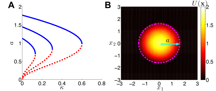
Fig. 1: Stationary bump solutions u(𝐱,t)=U(r)𝑢𝐱𝑡𝑈𝑟u({\mathbf{x}},t)=U(r) to the deterministic model (1) with weight function (2) and Heaviside firing rate (4). (A) A wider stable (solid) and narrower unstable (dashed) branch of solutions to U(a)=κ𝑈𝑎𝜅U(a)=\kappa emerges from a saddle-node bifurcation at a critical value of κ𝜅\kappa above which no solutions exist. Weight function parameters are (left to right) [c1,c2,c3,c4]=[10/9,10/9,1/3,1/3];[4/3,4/3,2/5,1/3];[5/3,5/3,1/2,1/2]subscript𝑐1subscript𝑐2subscript𝑐3subscript𝑐410910913134343251353531212[c_{1},c_{2},c_{3},c_{4}]=[10/9,-10/9,-1/3,1/3];[4/3,-4/3,-2/5,1/3];[5/3,-5/3,-1/2,1/2]. (B) An example of a stationary bump U(𝐱)𝑈𝐱U({\mathbf{x}}) for the parameters κ=0.2𝜅0.2\kappa=0.2 and [c1,c2,c3,c4]=[5/3,5/3,1/2,1/2]subscript𝑐1subscript𝑐2subscript𝑐3subscript𝑐453531212[c_{1},c_{2},c_{3},c_{4}]=[5/3,-5/3,-1/2,1/2]. We have fixed [α1,α2,α3,α4]=[1,2,1/4,1/2]subscript𝛼1subscript𝛼2subscript𝛼3subscript𝛼4121412[\alpha_{1},\alpha_{2},\alpha_{3},\alpha_{4}]=[1,2,1/4,1/2], as in (19).

To illustrate our analysis, we consider the weight (2) given by a sum of modified Bessel functions [44]. Using the fact that the corresponding Hankel transform of K0(sr)subscript𝐾0𝑠𝑟K_{0}(sr) is (ρ,s)=(ρ2+s2)1𝜌𝑠superscriptsuperscript𝜌2superscript𝑠21{\mathcal{H}}(\rho,s)=(\rho^{2}+s^{2})^{-1}, we have

w^(ρ)=j=1Ncj(ρ,αj).^𝑤𝜌superscriptsubscript𝑗1𝑁subscript𝑐𝑗𝜌subscript𝛼𝑗\displaystyle\widehat{w}(\rho)=\sum_{j=1}^{N}c_{j}{\mathcal{H}}(\rho,\alpha_{j}). (14)

The bump solution (13) can then be evaluated by using the formula (14) along with the identity

0J0(ρr)J1(ρa)ρ2+s2𝑑ρ(a,r,s)={1sI1(sa)K0(sr):r>a,1s2a1sI0(sr)K1(sa):r<a,superscriptsubscript0subscript𝐽0𝜌𝑟subscript𝐽1𝜌𝑎superscript𝜌2superscript𝑠2differential-d𝜌𝑎𝑟𝑠cases1𝑠subscript𝐼1𝑠𝑎subscript𝐾0𝑠𝑟:absent𝑟𝑎1superscript𝑠2𝑎1𝑠subscript𝐼0𝑠𝑟subscript𝐾1𝑠𝑎:absent𝑟𝑎\displaystyle\int_{0}^{\infty}\frac{J_{0}(\rho r)J_{1}(\rho a)}{\rho^{2}+s^{2}}d\rho\equiv{\mathcal{I}}(a,r,s)=\left\{\begin{array}[]{ll}\frac{1}{s}I_{1}(sa)K_{0}(sr)&:r>a,\\ \frac{1}{s^{2}a}-\frac{1}{s}I_{0}(sr)K_{1}(sa)&:r<a,\end{array}\right. (17)

where Iνsubscript𝐼𝜈I_{\nu} is the modified Bessel function of the first kind of order ν𝜈\nu. We can thus generate an explicit solution for the stationary bump U(r)𝑈𝑟U(r), given

U(r)=2πak=0Nck(a,r,αk).𝑈𝑟2𝜋𝑎superscriptsubscript𝑘0𝑁subscript𝑐𝑘𝑎𝑟subscript𝛼𝑘\displaystyle U(r)=2\pi a\sum_{k=0}^{N}c_{k}{\mathcal{I}}(a,r,\alpha_{k}).

Applying the threshold condition U(a)=κ𝑈𝑎𝜅U(a)=\kappa, we can generate an implicit equation relating the bump radius a𝑎a with the threshold κ𝜅\kappa and weight parameters

U(a)=2πak=0NckαkI1(αka)K0(αka)=κ.𝑈𝑎2𝜋𝑎superscriptsubscript𝑘0𝑁subscript𝑐𝑘subscript𝛼𝑘subscript𝐼1subscript𝛼𝑘𝑎subscript𝐾0subscript𝛼𝑘𝑎𝜅U(a)=2\pi a\sum_{k=0}^{N}\frac{c_{k}}{\alpha_{k}}I_{1}(\alpha_{k}a)K_{0}(\alpha_{k}a)=\kappa. (18)

In general, explicit solutions for a𝑎a cannot be computed and (18) must be solved numerically using root finding algorithms. Note also that satisfaction of the threshold condition (18) is not sufficient for proving the existence of a bump. For instance, the possibility of ring solutions must be eliminated by ensuring there are no other threshold crossing points [44, 18]. Furthermore, we must develop a linear stability analysis to identify those bumps that will persist in the presence of perturbations. This will especially be important in our analysis of the stochastic system (5), since it will rely on the assumption that the perturbed solutions retains a profile similar to the unperturbed system.

We demonstrate the results of this existence analysis by utilizing a Mexican hat type weight distributions such as [44, 11]

w(r)=c1K0(r)+c2K0(2r)+c3K0(r/4)+c4K0(r/2),𝑤𝑟subscript𝑐1subscript𝐾0𝑟subscript𝑐2subscript𝐾02𝑟subscript𝑐3subscript𝐾0𝑟4subscript𝑐4subscript𝐾0𝑟2\displaystyle w(r)=c_{1}K_{0}(r)+c_{2}K_{0}(2r)+c_{3}K_{0}(r/4)+c_{4}K_{0}(r/2), (19)

where we have fixed the spatial scales [α1,α2,α3,α4]=[1,2,1/4,1/2]subscript𝛼1subscript𝛼2subscript𝛼3subscript𝛼4121412[\alpha_{1},\alpha_{2},\alpha_{3},\alpha_{4}]=[1,2,1/4,1/2] and will take c1,c4>0subscript𝑐1subscript𝑐40c_{1},c_{4}>0 and c2,c3<0subscript𝑐2subscript𝑐30c_{2},c_{3}<0 to generate a lateral inhibitory kernel. Typically, weight functions like (19) lead to a maximum of two bump solutions, as shown in Fig. 1.

As mentioned, we must be aware of the possibility of azimuthal instabilities of the stationary bump when developing our linear stability theory [44, 9]. Thus, while it may be convenient to analogize the shifting and expanding/contracting perturbations of 1D bumps [2] with D1subscript𝐷1D_{1} and circularly symmetric perturbations of 2D bumps [47], one should be sure not to stop here. A full analysis of azimuthal perturbations to the bump (11), Dnsubscript𝐷𝑛D_{n}-symmetric perturbations (n𝑛n\in\mathbb{Z}, n>1𝑛1n>1), is necessary since bumps can destabilize through such symmetry-breaking instabilities [44, 11]. It is worth noting that this fact was originally identified by Amari in 1978 [4], and other systematic analyses were carried out in the last decade [44, 18].

To determine the stability of stationary solution, we will consider small, smooth perturbations of the stationary bump solution (11) of the form u(𝐱,t):=U(𝐱)+εΨ(𝐱,t)assign𝑢𝐱𝑡𝑈𝐱𝜀Ψ𝐱𝑡u({\mathbf{x}},t):=U({\mathbf{x}})+\varepsilon\Psi({\mathbf{x}},t) where ε1much-less-than𝜀1\varepsilon\ll 1. We substitute this into equation (1) and Taylor expand to linear order to generate the equation

Ψ(𝐱,t)t=Ψ(𝐱,𝐭)+2w(𝐱𝐲)f(U(𝐲))Ψ(𝐲,t)𝑑𝐲.Ψ𝐱𝑡𝑡Ψ𝐱𝐭subscriptsuperscript2𝑤𝐱𝐲superscript𝑓𝑈𝐲Ψ𝐲𝑡differential-d𝐲\frac{\partial\Psi({\mathbf{x}},t)}{\partial t}=-\Psi(\mathbf{x,t})+\int_{\mathbb{R}^{2}}w({\mathbf{x}}-\mathbf{y})f^{\prime}(U(\mathbf{y}))\Psi(\mathbf{y},t)d\mathbf{y}. (20)

Applying seperation of variables Ψ(𝐱,t)=Ψ(𝐱)b(t)Ψ𝐱𝑡Ψ𝐱𝑏𝑡\Psi({\mathbf{x}},t)=\Psi({\mathbf{x}})b(t) and rearranging terms results in the solutions b(t)=eλt𝑏𝑡superscript𝑒𝜆𝑡b(t)=e^{\lambda t} and

(λ+1)Ψ(𝐱)=2w(𝐱𝐲)f(U(𝐲))Ψ(𝐲)𝑑𝐲.𝜆1Ψ𝐱subscriptsuperscript2𝑤𝐱𝐲superscript𝑓𝑈𝐲Ψ𝐲differential-d𝐲(\lambda+1)\Psi({\mathbf{x}})=\int_{\mathbb{R}^{2}}w({\mathbf{x}}-\mathbf{y})f^{\prime}(U(\mathbf{y}))\Psi(\mathbf{y})d\mathbf{y}. (21)

We can immediately identify neutrally stable perturbations, those corresponding to λ=0𝜆0\lambda=0, by letting Ψ(𝐱)=Uxj(𝐱)Ψ𝐱subscript𝑈subscript𝑥𝑗𝐱\Psi({\mathbf{x}})=U_{x_{j}}({\mathbf{x}}) with j{1,2}𝑗12j\in\{1,2\}. We apply integration by parts and the definition of a stationary solution U𝑈U given in (10) into (21) to yield

(λ+1)Uxj(𝐱)𝜆1subscript𝑈subscript𝑥𝑗𝐱\displaystyle(\lambda+1)U_{x_{j}}({\mathbf{x}}) =2w(𝐱𝐲)f(U(𝐲))Uyj(𝐲)𝑑𝐲=2w(𝐱𝐲)yj(f(U(𝐲)))𝑑𝐲absentsubscriptsuperscript2𝑤𝐱𝐲superscript𝑓𝑈𝐲subscript𝑈subscript𝑦𝑗𝐲differential-d𝐲subscriptsuperscript2𝑤𝐱𝐲subscript𝑦𝑗𝑓𝑈𝐲differential-d𝐲\displaystyle=\int_{\mathbb{R}^{2}}w({\mathbf{x}}-\mathbf{y})f^{\prime}(U(\mathbf{y}))U_{y_{j}}(\mathbf{y})\;d\mathbf{y}=\int_{\mathbb{R}^{2}}w({\mathbf{x}}-\mathbf{y})\frac{\partial}{\partial y_{j}}\big{(}f(U(\mathbf{y}))\big{)}\;d\mathbf{y}
=2yj(w(𝐱𝐲))f(U(𝐲))𝑑𝐲=2xj(w(𝐱𝐲))f(U(𝐲))𝑑𝐲absentsubscriptsuperscript2subscript𝑦𝑗𝑤𝐱𝐲𝑓𝑈𝐲differential-d𝐲subscriptsuperscript2subscript𝑥𝑗𝑤𝐱𝐲𝑓𝑈𝐲differential-d𝐲\displaystyle=\int_{\mathbb{R}^{2}}\frac{\partial}{\partial y_{j}}\big{(}w({\mathbf{x}}-\mathbf{y})\big{)}f(U(\mathbf{y}))\;d\mathbf{y}=\int_{\mathbb{R}^{2}}\frac{\partial}{\partial x_{j}}\big{(}w({\mathbf{x}}-\mathbf{y})\big{)}f(U(\mathbf{y}))\;d\mathbf{y}
=xj(2w(𝐱𝐲)f(U(𝐲))𝑑𝐲)=Uxj(𝐱).absentsubscript𝑥𝑗subscriptsuperscript2𝑤𝐱𝐲𝑓𝑈𝐲differential-d𝐲subscript𝑈subscript𝑥𝑗𝐱\displaystyle=\frac{\partial}{\partial x_{j}}\bigg{(}\int_{\mathbb{R}^{2}}w({\mathbf{x}}-\mathbf{y})f(U(\mathbf{y}))\;d\mathbf{y}\bigg{)}=U_{x_{j}}({\mathbf{x}}). (22)

Thus, by the linearity of the integral

ΨZ(𝐱)=h1Ux1(𝐱)+h2Ux2(𝐱)subscriptΨ𝑍𝐱subscript1subscript𝑈subscript𝑥1𝐱subscript2subscript𝑈subscript𝑥2𝐱\displaystyle\Psi_{Z}({\mathbf{x}})=h_{1}U_{x_{1}}({\mathbf{x}})+h_{2}U_{x_{2}}({\mathbf{x}}) (23)

generates the class of solutions corresponding to the eigenvalue λ1=0subscript𝜆10\lambda_{1}=0. Note, we will not have such a class of perturbations in the case of stationary external inputs, as the translation symmetry of (1) will then be broken.

Prior to analyzing other azimuthal perturbations to the bump (11), we briefly discuss how perturbations of the form (23) impact the long term bump position. In fact, it is precisely this neutral stability of the bump that leads to purely diffusive motion of the bump in the stochastic model (5). Specifically, we focus on the case of a Heaviside firing rate function (4), so we can track the position 𝚫=(Δ1,Δ2)2𝚫subscriptΔ1subscriptΔ2superscript2{\bm{\Delta}}=(\Delta_{1},\Delta_{2})\in{\mathbb{R}}^{2}, i.e. the spatial mean, of the bump by utilizing the level set condition u(𝐱,t)=κ𝑢𝐱𝑡𝜅u({\mathbf{x}},t)=\kappa, which can be written

κ=𝜅absent\displaystyle\kappa= u(a+εb(θ,t),θ,t)=U(a+εb(θ,t))+εΨ(a+εb(θ,t),θ,t)𝑢𝑎𝜀𝑏𝜃𝑡𝜃𝑡𝑈𝑎𝜀𝑏𝜃𝑡𝜀Ψ𝑎𝜀𝑏𝜃𝑡𝜃𝑡\displaystyle u(a+\varepsilon b(\theta,t),\theta,t)=U(a+\varepsilon b(\theta,t))+\varepsilon\Psi(a+\varepsilon b(\theta,t),\theta,t)
κ=𝜅absent\displaystyle\kappa= U(a)+εU(a)b(θ,t)+εΨ(a,θ,t)+𝒪(ε2),𝑈𝑎𝜀superscript𝑈𝑎𝑏𝜃𝑡𝜀Ψ𝑎𝜃𝑡𝒪superscript𝜀2\displaystyle U(a)+\varepsilon U^{\prime}(a)b(\theta,t)+\varepsilon\Psi(a,\theta,t)+{\mathcal{O}}(\varepsilon^{2}), (24)

where b(θ,t)𝑏𝜃𝑡b(\theta,t) describes the perturbation of the bump boundary R(θ,t)=a+εb(θ,t)𝑅𝜃𝑡𝑎𝜀𝑏𝜃𝑡R(\theta,t)=a+\varepsilon b(\theta,t) at angular coordinate θ𝜃\theta and ε1much-less-than𝜀1\varepsilon\ll 1. Note we can employ the stationary level set condition U(a)=κ𝑈𝑎𝜅U(a)=\kappa to cancel leading order terms in (24) to yield [24]

b(θ,t)=Ψ(a,θ,t)|U(a)|+𝒪(ε).𝑏𝜃𝑡Ψ𝑎𝜃𝑡superscript𝑈𝑎𝒪𝜀\displaystyle b(\theta,t)=\frac{\Psi(a,\theta,t)}{|U^{\prime}(a)|}+{\mathcal{O}}(\varepsilon). (25)

If we specifically denote Ψ(a,θ,t)Ψ𝑎𝜃𝑡\Psi(a,\theta,t) to be a neutrally stable perturbation (23), then Ψ(a,θ,t)=ΨZ(a,θ)Ψ𝑎𝜃𝑡subscriptΨ𝑍𝑎𝜃\Psi(a,\theta,t)=\Psi_{Z}(a,\theta) and b(θ,t)=b1(θ)𝑏𝜃𝑡subscript𝑏1𝜃b(\theta,t)=b_{1}(\theta), so that to first order

b1(θ)=ΨZ(a,θ)|U(a)|=h1U(a)cosθ+h2U(a)sinθ|U(a)|=h1cosθh2sinθ,subscript𝑏1𝜃subscriptΨ𝑍𝑎𝜃superscript𝑈𝑎subscript1superscript𝑈𝑎𝜃subscript2superscript𝑈𝑎𝜃superscript𝑈𝑎subscript1𝜃subscript2𝜃\displaystyle b_{1}(\theta)=\frac{\Psi_{Z}(a,\theta)}{|U^{\prime}(a)|}=\frac{h_{1}U^{\prime}(a)\cos\theta+h_{2}U^{\prime}(a)\sin\theta}{|U^{\prime}(a)|}=-h_{1}\cos\theta-h_{2}\sin\theta, (26)

where we have computed

x1U(𝐱)|r=a=U(a)cosθ,x2U(𝐱)|r=a=U(a)sinθ.formulae-sequenceevaluated-atsubscript𝑥1𝑈norm𝐱𝑟𝑎superscript𝑈𝑎𝜃evaluated-atsubscript𝑥2𝑈norm𝐱𝑟𝑎superscript𝑈𝑎𝜃\displaystyle\left.\frac{\partial}{\partial x_{1}}U(||{\mathbf{x}}||)\right|_{r=a}=U^{\prime}(a)\cos\theta,\hskip 28.45274pt\left.\frac{\partial}{\partial x_{2}}U(||{\mathbf{x}}||)\right|_{r=a}=U^{\prime}(a)\sin\theta. (27)

Thus, the new bump boundary R0(θ)a+εb1(θ)subscript𝑅0𝜃𝑎𝜀subscript𝑏1𝜃R_{0}(\theta)\approx a+\varepsilon b_{1}(\theta) can be approximated in polar coordinates as

R0(θ)=aεh1cosθεh2sinθ.subscript𝑅0𝜃𝑎𝜀subscript1𝜃𝜀subscript2𝜃\displaystyle R_{0}(\theta)=a-\varepsilon h_{1}\cos\theta-\varepsilon h_{2}\sin\theta. (28)

This approximates the long-term perturbation to the bump boundary limtR(θ,t)R0(θ)subscript𝑡𝑅𝜃𝑡subscript𝑅0𝜃\lim_{t\to\infty}R(\theta,t)\approx R_{0}(\theta) by simply using the leading order term in the expansion b(θ,t)=b1(θ)+j=0,j1bj(θ)eλjt𝑏𝜃𝑡subscript𝑏1𝜃superscriptsubscriptformulae-sequence𝑗0𝑗1subscript𝑏𝑗𝜃superscriptesubscript𝜆𝑗𝑡b(\theta,t)=b_{1}(\theta)+\sum_{j=0,j\neq 1}^{\infty}b_{j}(\theta){\rm e}^{\lambda_{j}t}, as limtb(θ,t)=b1(θ)subscript𝑡𝑏𝜃𝑡subscript𝑏1𝜃\lim_{t\to\infty}b(\theta,t)=b_{1}(\theta) since all other Reλj<0Resubscript𝜆𝑗0{\rm Re}\lambda_{j}<0. This utilizes the well known result that circularly symmetric bump solutions to (1) are neutrally stable to D1subscript𝐷1D_{1} symmetric perturbations of the bump boundary [24, 44]. Now, define the centroid (center of mass) 𝚫=(Δ1,Δ2)𝚫subscriptΔ1subscriptΔ2{\bm{\Delta}}=(\Delta_{1},\Delta_{2}) as the first moments of mass along the xlimit-from𝑥x- and ylimit-from𝑦y-directions scaled by the total mass for the lamina ΩRsubscriptΩ𝑅\Omega_{R} of uniform density enclosed by the curve (28). In Cartesian coordinates, these quantities are given by the double integral formulae Δ1=ΩRx𝑑x𝑑y/ΩR𝑑x𝑑ysubscriptΔ1subscriptsubscriptΩ𝑅𝑥differential-d𝑥differential-d𝑦subscriptsubscriptΩ𝑅differential-d𝑥differential-d𝑦\Delta_{1}=\int\int_{\Omega_{R}}xdxdy/\int\int_{\Omega_{R}}dxdy and Δ2=ΩRy𝑑x𝑑y/ΩR𝑑x𝑑ysubscriptΔ2subscriptsubscriptΩ𝑅𝑦differential-d𝑥differential-d𝑦subscriptsubscriptΩ𝑅differential-d𝑥differential-d𝑦\Delta_{2}=\int\int_{\Omega_{R}}ydxdy/\int\int_{\Omega_{R}}dxdy. By utilizing polar coordinates (x,y)=(rcosθ,rsinθ)𝑥𝑦𝑟𝜃𝑟𝜃(x,y)=(r\cos\theta,r\sin\theta), and plugging in the formula for the closed curve R(θ)𝑅𝜃R(\theta) (28), we can compute:

Δ1subscriptΔ1\displaystyle\Delta_{1} =02π0R(θ)r2cosθdrdθ02π0R(θ)r𝑑r𝑑θ=1302π(aεh1cosθεh2sinθ)3cosθdθ1202π(aεh1cosθεh2sinθ)2𝑑θabsentsuperscriptsubscript02𝜋superscriptsubscript0𝑅𝜃superscript𝑟2𝜃𝑑𝑟𝑑𝜃superscriptsubscript02𝜋superscriptsubscript0𝑅𝜃𝑟differential-d𝑟differential-d𝜃13superscriptsubscript02𝜋superscript𝑎𝜀subscript1𝜃𝜀subscript2𝜃3𝜃𝑑𝜃12superscriptsubscript02𝜋superscript𝑎𝜀subscript1𝜃𝜀subscript2𝜃2differential-d𝜃\displaystyle=\frac{\int_{0}^{2\pi}\int_{0}^{R(\theta)}r^{2}\cos\theta drd\theta}{\int_{0}^{2\pi}\int_{0}^{R(\theta)}rdrd\theta}=\frac{\frac{1}{3}\int_{0}^{2\pi}(a-\varepsilon h_{1}\cos\theta-\varepsilon h_{2}\sin\theta)^{3}\cos\theta d\theta}{\frac{1}{2}\int_{0}^{2\pi}(a-\varepsilon h_{1}\cos\theta-\varepsilon h_{2}\sin\theta)^{2}d\theta}
=a2302π(a3εh1cosθ3εh2sinθ)cosθdθa202π(a2εh1cosθ2εh2sinθ)𝑑θ+𝒪(ε2)εh1absentsuperscript𝑎23superscriptsubscript02𝜋𝑎3𝜀subscript1𝜃3𝜀subscript2𝜃𝜃𝑑𝜃𝑎2superscriptsubscript02𝜋𝑎2𝜀subscript1𝜃2𝜀subscript2𝜃differential-d𝜃𝒪superscript𝜀2𝜀subscript1\displaystyle=\frac{\frac{a^{2}}{3}\int_{0}^{2\pi}\left(a-3\varepsilon h_{1}\cos\theta-3\varepsilon h_{2}\sin\theta\right)\cos\theta d\theta}{\frac{a}{2}\int_{0}^{2\pi}\left(a-2\varepsilon h_{1}\cos\theta-2\varepsilon h_{2}\sin\theta\right)d\theta}+{\mathcal{O}}(\varepsilon^{2})\approx-\varepsilon h_{1}

and

Δ2subscriptΔ2\displaystyle\Delta_{2} =02π0R(θ)r2sinθdrdθ02π0R(θ)r𝑑r𝑑θ=1302π(aεh1cosθεh2sinθ)3sinθdθ1202π(aεh1cosθεh2sinθ)2𝑑θabsentsuperscriptsubscript02𝜋superscriptsubscript0𝑅𝜃superscript𝑟2𝜃𝑑𝑟𝑑𝜃superscriptsubscript02𝜋superscriptsubscript0𝑅𝜃𝑟differential-d𝑟differential-d𝜃13superscriptsubscript02𝜋superscript𝑎𝜀subscript1𝜃𝜀subscript2𝜃3𝜃𝑑𝜃12superscriptsubscript02𝜋superscript𝑎𝜀subscript1𝜃𝜀subscript2𝜃2differential-d𝜃\displaystyle=\frac{\int_{0}^{2\pi}\int_{0}^{R(\theta)}r^{2}\sin\theta drd\theta}{\int_{0}^{2\pi}\int_{0}^{R(\theta)}rdrd\theta}=\frac{\frac{1}{3}\int_{0}^{2\pi}(a-\varepsilon h_{1}\cos\theta-\varepsilon h_{2}\sin\theta)^{3}\sin\theta d\theta}{\frac{1}{2}\int_{0}^{2\pi}(a-\varepsilon h_{1}\cos\theta-\varepsilon h_{2}\sin\theta)^{2}d\theta}
=a2302π(a3εh1cosθ3εh2sinθ)sinθdθa202π(a2εh1cosθ2εh2sinθ)𝑑θ+𝒪(ε2)εh2.absentsuperscript𝑎23superscriptsubscript02𝜋𝑎3𝜀subscript1𝜃3𝜀subscript2𝜃𝜃𝑑𝜃𝑎2superscriptsubscript02𝜋𝑎2𝜀subscript1𝜃2𝜀subscript2𝜃differential-d𝜃𝒪superscript𝜀2𝜀subscript2\displaystyle=\frac{\frac{a^{2}}{3}\int_{0}^{2\pi}\left(a-3\varepsilon h_{1}\cos\theta-3\varepsilon h_{2}\sin\theta\right)\sin\theta d\theta}{\frac{a}{2}\int_{0}^{2\pi}\left(a-2\varepsilon h_{1}\cos\theta-2\varepsilon h_{2}\sin\theta\right)d\theta}+{\mathcal{O}}(\varepsilon^{2})\approx-\varepsilon h_{2}.

Thus a perturbation in the bump profile of the form (23) will yield a proportional shift in the bump’s center of mass (Δ1,Δ2)=ε(h1,h2)subscriptΔ1subscriptΔ2𝜀subscript1subscript2(\Delta_{1},\Delta_{2})=-\varepsilon(h_{1},h_{2}). This foreshadows the impact of noise-induced perturbations to the bump’s position, which we explore in section 3.2. Effectively, we will show the primary contribution to the stochastic motion of bumps is the D1subscript𝐷1D_{1}-symmetric portion of the spatiotemporal noise, which is filtered by the bump as a spatial translation of its boundary and center of mass.

Lastly, we briefly review the analysis of azimuthal perturbations to the bump boundary. Note that in the case of a Heaviside firing rate function (4), then

f(U(𝐱))=δ(U(r)κ)=δ(ra)|U(a)|,superscript𝑓𝑈𝐱𝛿𝑈𝑟𝜅𝛿𝑟𝑎superscript𝑈𝑎\displaystyle f^{\prime}(U({\mathbf{x}}))=\delta(U(r)-\kappa)=\frac{\delta(r-a)}{|U^{\prime}(a)|}, (29)

where U(a)superscript𝑈𝑎U^{\prime}(a) is the normal derivative of U(𝐱)𝑈𝐱U({\mathbf{x}}) along the bump boundary r=a𝑟𝑎r=a, in polar coordinates 𝐫=(r,θ)𝐫𝑟𝜃{\mathbf{r}}=(r,\theta). Thus, the eigenvalue equation (21) becomes

(λ+1)Ψ(𝐫)=a|U(a)|02πw(|𝐫𝐚|)Ψ(a,θ)𝑑θ,𝜆1Ψ𝐫𝑎superscript𝑈𝑎superscriptsubscript02𝜋𝑤𝐫superscript𝐚Ψ𝑎superscript𝜃differential-dsuperscript𝜃\displaystyle(\lambda+1)\Psi({\mathbf{r}})=\frac{a}{|U^{\prime}(a)|}\int_{0}^{2\pi}w(|{\mathbf{r}}-{\mathbf{a}}^{\prime}|)\Psi(a,\theta^{\prime})d\theta^{\prime}, (30)

where 𝐚=(a,θ)superscript𝐚𝑎superscript𝜃{\mathbf{a}}^{\prime}=(a,\theta^{\prime}) in polar coordinates, equivalently 𝐚=a(cosθ,sinθ)superscript𝐚𝑎𝜃𝜃{\mathbf{a}}^{\prime}=a(\cos\theta,\sin\theta) in Cartesian coordinates. Stability of the bump is thus determined by the spectrum of a compact linear operator acting on continuous, bounded functions Ψ(r,θ)Ψ𝑟𝜃\Psi(r,\theta) defined on the disc of radius ra𝑟𝑎r\leq a. The essential spectrum contains functions Ψ(𝐫)Ψ𝐫\Psi({\mathbf{r}}) that vanish on the boundary Ψ(a,θ)=0Ψ𝑎𝜃0\Psi(a,\theta)=0 for all θ𝜃\theta, so λ=1𝜆1\lambda=-1, contributing to no instabilities. We can thus identify the discrete spectrum by setting 𝐫=𝐚=(a,θ)𝐫𝐚𝑎𝜃{\mathbf{r}}={\mathbf{a}}=(a,\theta) in (30), so

(λ+1)Ψ(a,θ)=a|U(a)|02πw(2asin(θθ2))Ψ(a,θ)𝑑θ,𝜆1Ψ𝑎𝜃𝑎superscript𝑈𝑎superscriptsubscript02𝜋𝑤2𝑎𝜃superscript𝜃2Ψ𝑎superscript𝜃differential-dsuperscript𝜃\displaystyle(\lambda+1)\Psi(a,\theta)=\frac{a}{|U^{\prime}(a)|}\int_{0}^{2\pi}w\left(2a\sin\left(\frac{\theta-\theta^{\prime}}{2}\right)\right)\Psi(a,\theta^{\prime})d\theta^{\prime},

where we have utilized the identity

|𝐚𝐚|=2a22a2cos(θθ)=2asin(θθ2).𝐚superscript𝐚2superscript𝑎22superscript𝑎2𝜃superscript𝜃2𝑎𝜃superscript𝜃2\displaystyle|{\mathbf{a}}-{\mathbf{a}}^{\prime}|=\sqrt{2a^{2}-2a^{2}\cos(\theta-\theta^{\prime})}=2a\sin\left(\frac{\theta-\theta^{\prime}}{2}\right).

Any perturbation can be decomposed into the infinite series of Fourier modes Ψ(a,θ)=n=0AnΨn(θ)+BnΨn¯(θ)Ψ𝑎𝜃superscriptsubscript𝑛0subscript𝐴𝑛subscriptΨ𝑛𝜃subscript𝐵𝑛¯subscriptΨ𝑛𝜃\Psi(a,\theta)=\sum_{n=0}^{\infty}A_{n}\Psi_{n}(\theta)+B_{n}\bar{\Psi_{n}}(\theta), where Ψn(θ)=einθsubscriptΨ𝑛𝜃superscripte𝑖𝑛𝜃\Psi_{n}(\theta)={\rm e}^{in\theta} and Ψ¯n(θ)=einθsubscript¯Ψ𝑛𝜃superscripte𝑖𝑛𝜃\bar{\Psi}_{n}(\theta)={\rm e}^{-in\theta} [23, 44]. We can thus compute all the eigenvalues of the discrete spectrum by evaluating the expression

λn=1+a|U(a)|02πw(2asin(θ/2))einθsubscript𝜆𝑛1𝑎superscript𝑈𝑎superscriptsubscript02𝜋𝑤2𝑎𝜃2superscripte𝑖𝑛𝜃\displaystyle\lambda_{n}=-1+\frac{a}{|U^{\prime}(a)|}\int_{0}^{2\pi}w(2a\sin(\theta/2)){\rm e}^{-in\theta}

each associated with Ψn(θ)subscriptΨ𝑛𝜃\Psi_{n}(\theta) for n0𝑛subscriptabsent0n\in\mathbb{Z}_{\geq 0}. Note, λnsubscript𝜆𝑛\lambda_{n} will always be real, since rescaling θ2θmaps-to𝜃2𝜃\theta\mapsto 2\theta:

Im{λn}=2a|U(a)|0πw(2asinθ)sin(2nθ)𝑑θ=0.Imsubscript𝜆𝑛2𝑎superscript𝑈𝑎superscriptsubscript0𝜋𝑤2𝑎𝜃2𝑛𝜃differential-d𝜃0\displaystyle{\rm Im}\{\lambda_{n}\}=-\frac{2a}{|U^{\prime}(a)|}\int_{0}^{\pi}w(2a\sin\theta)\sin(2n\theta)d\theta=0.

Therefore, the eigenvalue is real

λn=Re{λn}=1+a|U(a)|02πw(2asin(θ/2))cos(nθ)𝑑θ.subscript𝜆𝑛Resubscript𝜆𝑛1𝑎superscript𝑈𝑎superscriptsubscript02𝜋𝑤2𝑎𝜃2𝑛𝜃differential-d𝜃\displaystyle\lambda_{n}={\rm Re}\{\lambda_{n}\}=-1+\frac{a}{|U^{\prime}(a)|}\int_{0}^{2\pi}w(2a\sin(\theta/2))\cos(n\theta)d\theta. (31)

Note, the bump profile perturbation Ψ(𝐫,t)Ψ𝐫𝑡\Psi({\mathbf{r}},t) will be related to the bump boundary perturbation b(θ,t)𝑏𝜃𝑡b(\theta,t) via the formula (25), as discussed above. The n𝑛nth order boundary perturbation has Dnsubscript𝐷𝑛D_{n} symmetry; e.g. n=0𝑛0n=0 uniformly expands/contracts the bump, n=1𝑛1n=1 shifts the bump.

By specifying the weight function w(r)𝑤𝑟w(r), we can compute the eigenvalue (31) explicitly using Bessel functions to evaluate the integral

02πw(|𝐚𝐚|)cos(nθ)𝑑θsuperscriptsubscript02𝜋𝑤𝐚superscript𝐚𝑛superscript𝜃differential-dsuperscript𝜃\displaystyle\int_{0}^{2\pi}w(|{\mathbf{a}}-{\mathbf{a}}^{\prime}|)\cos(n\theta^{\prime})d\theta^{\prime} =02π(0w^(ρ)J0(ρ|𝐚𝐚|)ρ𝑑ρ)cosθdθabsentsuperscriptsubscript02𝜋superscriptsubscript0^𝑤𝜌subscript𝐽0𝜌𝐚superscript𝐚𝜌differential-d𝜌superscript𝜃𝑑superscript𝜃\displaystyle=\int_{0}^{2\pi}\left(\int_{0}^{\infty}\widehat{w}(\rho)J_{0}(\rho|{\mathbf{a}}-{\mathbf{a}}^{\prime}|)\rho d\rho\right)\cos\theta^{\prime}d\theta^{\prime}
=2π0w^(ρ)Jn(ρr)Jn(ρa)ρ𝑑ρ.absent2𝜋superscriptsubscript0^𝑤𝜌subscript𝐽𝑛𝜌𝑟subscript𝐽𝑛𝜌𝑎𝜌differential-d𝜌\displaystyle=2\pi\int_{0}^{\infty}\widehat{w}(\rho)J_{n}(\rho r)J_{n}(\rho a)\rho d\rho.

Thus, we can write (31) as

λn=1+0w^(ρ)Jn(ρr)Jn(ρa)ρ𝑑ρ0w^(ρ)J1(ρr)J1(ρa)ρ𝑑ρ.subscript𝜆𝑛1superscriptsubscript0^𝑤𝜌subscript𝐽𝑛𝜌𝑟subscript𝐽𝑛𝜌𝑎𝜌differential-d𝜌superscriptsubscript0^𝑤𝜌subscript𝐽1𝜌𝑟subscript𝐽1𝜌𝑎𝜌differential-d𝜌\displaystyle\lambda_{n}=-1+\frac{\int_{0}^{\infty}\widehat{w}(\rho)J_{n}(\rho r)J_{n}(\rho a)\rho d\rho}{\int_{0}^{\infty}\widehat{w}(\rho)J_{1}(\rho r)J_{1}(\rho a)\rho d\rho}.

Since we know λ1=0subscript𝜆10\lambda_{1}=0, the bump will be stable if λn<0subscript𝜆𝑛0\lambda_{n}<0 for all n1𝑛1n\neq 1. Employing the general weight distribution (2), we find

λn=1+j=1NcjKn(αja)In(αja)j=1NcjK1(αja)I1(αja).subscript𝜆𝑛1superscriptsubscript𝑗1𝑁subscript𝑐𝑗subscript𝐾𝑛subscript𝛼𝑗𝑎subscript𝐼𝑛subscript𝛼𝑗𝑎superscriptsubscript𝑗1𝑁subscript𝑐𝑗subscript𝐾1subscript𝛼𝑗𝑎subscript𝐼1subscript𝛼𝑗𝑎\displaystyle\lambda_{n}=-1+\frac{\sum_{j=1}^{N}c_{j}K_{n}(\alpha_{j}a)I_{n}(\alpha_{j}a)}{\sum_{j=1}^{N}c_{j}K_{1}(\alpha_{j}a)I_{1}(\alpha_{j}a)}. (32)

More specifically, we could focus on the Mexican hat weight distribution (19) along with the parameters given in Fig. 1A. Indeed, checking the formula for the eigenvalues (32), we find λn<0subscript𝜆𝑛0\lambda_{n}<0 (n1𝑛1n\neq 1) for all solutions along the upper branch of wide bump solutions.

3.2 Effective equations for stochastic bump motion

We now explore how noise impacts the long term position of bumps in the network (5). Previous authors have analyzed the impact of noise on waves in reaction-diffusion [45, 5, 46] and neural field models [7, 8, 36] using small-noise expansions, but those studies tend to be on one-dimensional domains. Noise causes waves to execute an effective Brownian motion in their instantaneous position. As we will show, this analysis naturally extends to the effective stochastic dynamics of bumps in two-dimensional (2D) domains. The position 𝚫(t)=(Δ1(t),Δ2(t))𝚫𝑡subscriptΔ1𝑡subscriptΔ2𝑡{\bm{\Delta}}(t)=(\Delta_{1}(t),\Delta_{2}(t)) wanders diffusively, as a 2D random walk, as long as noise is small so that the profile of the bump remains close to the solution of the deterministic system (1). As mentioned, this relies upon the neutral stability of the noise free system; different behavior will arise when we break this symmetry with inputs, shown in section 4.

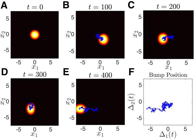
To begin, we assume that the weak additive noise (of 𝒪(ε1/2)𝒪superscript𝜀12{\mathcal{O}}(\varepsilon^{1/2})) in (5) affects the bump in two ways. Both are weak (𝒪(ε1/2)𝒪superscript𝜀12{\mathcal{O}}(\varepsilon^{1/2})) compared to the amplitude of the bump, allowing us to exploit regular perturbation theory to analyze the Langevin equation (5). First, the bump diffuses from its original position x𝑥x on long timescales according to the stochastic variable 𝚫(t)=(Δ1(t),Δ2(t))𝚫𝑡subscriptΔ1𝑡subscriptΔ2𝑡{\bm{\Delta}}(t)=(\Delta_{1}(t),\Delta_{2}(t)) (see Fig. 2, for example). Second, there are fluctuations in the bump profile on short timescales [5], according to the expansion ε1/2Φ+εΦ1+ε3/2Φ2+superscript𝜀12Φ𝜀subscriptΦ1superscript𝜀32subscriptΦ2\varepsilon^{1/2}\Phi+\varepsilon\Phi_{1}+\varepsilon^{3/2}\Phi_{2}+\cdots. This suggests the following ansatz for the impact of noise on the bump solution U(𝐱)𝑈𝐱U({\mathbf{x}}):

u(𝐱,t)=U(𝐱𝚫(t))+ε1/2Φ(𝐱𝚫(t),t)+.𝑢𝐱𝑡𝑈𝐱𝚫𝑡superscript𝜀12Φ𝐱𝚫𝑡𝑡u({\mathbf{x}},t)=U({\mathbf{x}}-{\bm{\Delta}}(t))+\varepsilon^{1/2}\Phi({\mathbf{x}}-{\bm{\Delta}}(t),t)+\cdots. (33)

Substituting (33) into (5) and truncating to 𝒪(1)𝒪1{\mathcal{O}}(1), we find that U(𝐱)𝑈𝐱U({\mathbf{x}}) still satisfies (10). Proceeding to linear order in ε1/2superscript𝜀12\varepsilon^{1/2}, we find

dΦ(𝐱,t)=Φ(𝐱,t)+ε1/2U(𝐱)d𝚫(t)+dW(𝐱,t),𝑑Φ𝐱𝑡Φ𝐱𝑡superscript𝜀12𝑈𝐱𝑑𝚫𝑡𝑑𝑊𝐱𝑡d\Phi({\mathbf{x}},t)={\mathcal{L}}\Phi({\mathbf{x}},t)+\varepsilon^{-1/2}\nabla U({\mathbf{x}})\cdot d{\bm{\Delta}}(t)+dW({\mathbf{x}},t), (34)

where U(𝐱)=(Ux1(𝐱),Ux2(𝐱))T𝑈𝐱superscriptsubscript𝑈subscript𝑥1𝐱subscript𝑈subscript𝑥2𝐱𝑇\nabla U({\mathbf{x}})=(U_{x_{1}}({\mathbf{x}}),U_{x_{2}}({\mathbf{x}}))^{T} denotes the gradient of U(𝐱)𝑈𝐱U({\mathbf{x}}) and {\mathcal{L}} is a non-self-adjoint linear operator of the form

p(𝐱)=p(𝐱)+2w(𝐱𝐲)f(U(𝐲))p(𝐲)𝑑𝐲𝑝𝐱𝑝𝐱subscriptsuperscript2𝑤𝐱𝐲superscript𝑓𝑈𝐲𝑝𝐲differential-d𝐲\displaystyle{\mathcal{L}}p({\mathbf{x}})=-p({\mathbf{x}})+\int_{{\mathbb{R}}^{2}}w({\mathbf{x}}-{\mathbf{y}})f^{\prime}(U({\mathbf{y}}))p({\mathbf{y}})d{\mathbf{y}} (35)

for any L2superscript𝐿2L^{2} integrable function p(𝐱)𝑝𝐱p({\mathbf{x}}) on 2superscript2{\mathbb{R}}^{2}. We ensure a bounded solution to (34) exists by requiring the inhomogeneous part is orthogonal to all elements of the null space of the adjoint operator superscript{\mathcal{L}}^{*}. The adjoint is defined by utilizing the L2superscript𝐿2L^{2} inner product

2[p(𝐱)]q(𝐱)𝑑𝐱=2p(𝐱)[q(𝐱)]𝑑𝐱,subscriptsuperscript2delimited-[]𝑝𝐱𝑞𝐱differential-d𝐱subscriptsuperscript2𝑝𝐱delimited-[]superscript𝑞𝐱differential-d𝐱\displaystyle\int_{{\mathbb{R}}^{2}}\left[{\mathcal{L}}p({\mathbf{x}})\right]q({\mathbf{x}})d{\mathbf{x}}=\int_{{\mathbb{R}}^{2}}p({\mathbf{x}})\left[{\mathcal{L}}^{*}q({\mathbf{x}})\right]d{\mathbf{x}},

where p(𝐱)𝑝𝐱p({\mathbf{x}}), q(𝐱)𝑞𝐱q({\mathbf{x}}) are L2superscript𝐿2L^{2} integrable on 2superscript2{\mathbb{R}}^{2}. Thus

q(𝐱)=q(𝐱)+f(U(𝐱))2w(𝐱𝐲)q(𝐲)𝑑𝐲.superscript𝑞𝐱𝑞𝐱superscript𝑓𝑈𝐱subscriptsuperscript2𝑤𝐱𝐲𝑞𝐲differential-d𝐲\displaystyle{\mathcal{L}}^{*}q({\mathbf{x}})=-q({\mathbf{x}})+f^{\prime}(U({\mathbf{x}}))\int_{{\mathbb{R}}^{2}}w({\mathbf{x}}-{\mathbf{y}})q({\mathbf{y}})d{\mathbf{y}}. (36)

The span of the nullspace of superscript{\mathcal{L}}^{*} can be described by two functions, which we can compute explicitly for a general firing rate function. That is, we can find an infinite number of solutions to the null space equation

φ(𝐱)=f(U(𝐱))2w(𝐱𝐲)φ(𝐲)𝑑𝐲,𝜑𝐱superscript𝑓𝑈𝐱subscriptsuperscript2𝑤𝐱𝐲𝜑𝐲differential-d𝐲\displaystyle\varphi({\mathbf{x}})=f^{\prime}(U({\mathbf{x}}))\int_{{\mathbb{R}}^{2}}w({\mathbf{x}}-{\mathbf{y}})\varphi({\mathbf{y}})d{\mathbf{y}}, (37)

which can always be decomposed into a linear combination of two functions φ1(𝐱)subscript𝜑1𝐱\varphi_{1}({\mathbf{x}}) and φ2(𝐱)subscript𝜑2𝐱\varphi_{2}({\mathbf{x}}). Specifically, we take φ1(𝐱)=f(U(𝐱))Ux1(𝐱)subscript𝜑1𝐱superscript𝑓𝑈𝐱subscript𝑈subscript𝑥1𝐱\varphi_{1}({\mathbf{x}})=f^{\prime}(U({\mathbf{x}}))U_{x_{1}}({\mathbf{x}}) and φ2(𝐱)=f(U(𝐱))Ux2(𝐱)subscript𝜑2𝐱superscript𝑓𝑈𝐱subscript𝑈subscript𝑥2𝐱\varphi_{2}({\mathbf{x}})=f^{\prime}(U({\mathbf{x}}))U_{x_{2}}({\mathbf{x}}), and note that by plugging into (37), we have

f(U(𝐱))Uxj(𝐱)=f(U(𝐱))2w(𝐱𝐲)f(U(𝐱))Uxj(𝐲)𝑑𝐲,superscript𝑓𝑈𝐱subscript𝑈subscript𝑥𝑗𝐱superscript𝑓𝑈𝐱subscriptsuperscript2𝑤𝐱𝐲superscript𝑓𝑈𝐱subscript𝑈subscript𝑥𝑗𝐲differential-d𝐲\displaystyle f^{\prime}(U({\mathbf{x}}))U_{x_{j}}({\mathbf{x}})=f^{\prime}(U({\mathbf{x}}))\int_{{\mathbb{R}}^{2}}w({\mathbf{x}}-{\mathbf{y}})f^{\prime}(U({\mathbf{x}}))U_{x_{j}}({\mathbf{y}})d{\mathbf{y}},

which holds due to to the equations in (22). Thus, we can derive an effective equation for the position variable 𝚫(t)𝚫𝑡{\bm{\Delta}}(t) by taking the inner product of φ1subscript𝜑1\varphi_{1} and φ2subscript𝜑2\varphi_{2} with both sides of (34) to yield

2f(U(𝐱))Ux1(𝐱)(Ux1(𝐱)dΔ1(t)+Ux2(𝐱)dΔ2(t)+ε1/2dW(𝐱,t))𝑑𝐱subscriptsuperscript2superscript𝑓𝑈𝐱subscript𝑈subscript𝑥1𝐱subscript𝑈subscript𝑥1𝐱𝑑subscriptΔ1𝑡subscript𝑈subscript𝑥2𝐱𝑑subscriptΔ2𝑡superscript𝜀12𝑑𝑊𝐱𝑡differential-d𝐱\displaystyle\int_{{\mathbb{R}}^{2}}f^{\prime}(U({\mathbf{x}}))U_{x_{1}}({\mathbf{x}})\left(U_{x_{1}}({\mathbf{x}})d\Delta_{1}(t)+U_{x_{2}}({\mathbf{x}})d\Delta_{2}(t)+\varepsilon^{1/2}dW({\mathbf{x}},t)\right)d{\mathbf{x}} =0absent0\displaystyle=0 (38)
2f(U(𝐱))Ux2(𝐱)(Ux1(𝐱)dΔ1(t)+Ux2(𝐱)dΔ2(t)+ε1/2dW(𝐱,t))𝑑𝐱subscriptsuperscript2superscript𝑓𝑈𝐱subscript𝑈subscript𝑥2𝐱subscript𝑈subscript𝑥1𝐱𝑑subscriptΔ1𝑡subscript𝑈subscript𝑥2𝐱𝑑subscriptΔ2𝑡superscript𝜀12𝑑𝑊𝐱𝑡differential-d𝐱\displaystyle\int_{{\mathbb{R}}^{2}}f^{\prime}(U({\mathbf{x}}))U_{x_{2}}({\mathbf{x}})\left(U_{x_{1}}({\mathbf{x}})d\Delta_{1}(t)+U_{x_{2}}({\mathbf{x}})d\Delta_{2}(t)+\varepsilon^{1/2}dW({\mathbf{x}},t)\right)d{\mathbf{x}} =0.absent0\displaystyle=0.

Moreover, we can exploit the odd and even symmetries of the spatial derivatives Ux1subscript𝑈subscript𝑥1U_{x_{1}} and Ux2subscript𝑈subscript𝑥2U_{x_{2}} that must hold since U(𝐱)𝑈𝐱U({\mathbf{x}}) is radially symmetric. Namely, Ux1subscript𝑈subscript𝑥1U_{x_{1}} is odd-symmetric along the x1subscript𝑥1x_{1}-axis and even along the x2subscript𝑥2x_{2}-axis, and Ux2subscript𝑈subscript𝑥2U_{x_{2}} is even-symmetric along the x1subscript𝑥1x_{1}-axis and odd along the x2subscript𝑥2x_{2}-axis. Lastly, f(U(𝐱))superscript𝑓𝑈𝐱f^{\prime}(U({\mathbf{x}})) is radially symmetric since U(𝐱)𝑈𝐱U({\mathbf{x}}) is. This means 2f(U(𝐱))Ux1(𝐱)Ux2(𝐱)𝑑𝐱=0subscriptsuperscript2superscript𝑓𝑈𝐱subscript𝑈subscript𝑥1𝐱subscript𝑈subscript𝑥2𝐱differential-d𝐱0\int_{{\mathbb{R}}^{2}}f^{\prime}(U({\mathbf{x}}))U_{x_{1}}({\mathbf{x}})U_{x_{2}}({\mathbf{x}})d{\mathbf{x}}=0. This allows us to rearrange the system (38), yielding a pair of independent equations for the diffusion of the bump along the x1subscript𝑥1x_{1} and x2subscript𝑥2x_{2} axes

dΔj(t)=ε1/22f(U(𝐱))Uxj(𝐱)𝑑W(𝐱,t)𝑑𝐱2f(U(𝐱))Uxj2(𝐱)𝑑𝐱,j{1,2}.formulae-sequence𝑑subscriptΔ𝑗𝑡superscript𝜀12subscriptsuperscript2superscript𝑓𝑈𝐱subscript𝑈subscript𝑥𝑗𝐱differential-d𝑊𝐱𝑡differential-d𝐱subscriptsuperscript2superscript𝑓𝑈𝐱superscriptsubscript𝑈subscript𝑥𝑗2𝐱differential-d𝐱𝑗12d\Delta_{j}(t)=-\varepsilon^{1/2}\frac{\int_{{\mathbb{R}}^{2}}f^{\prime}(U({\mathbf{x}}))U_{x_{j}}({\mathbf{x}})dW({\mathbf{x}},t)d{\mathbf{x}}}{\int_{{\mathbb{R}}^{2}}f^{\prime}(U({\mathbf{x}}))U_{x_{j}}^{2}({\mathbf{x}})d{\mathbf{x}}},\;\;\;\;j\in\{1,2\}. (39)

With the stochastic system (39) in hand, we can approximate the effective diffusivity of the bump. First, note that the mean position of the bump averaged across realizations does not change in time (𝚫(t)=(0,0)Tdelimited-⟨⟩𝚫𝑡superscript00𝑇\langle{\bm{\Delta}}(t)\rangle=(0,0)^{T}) since noise has mean zero (W(𝐱,t)=0delimited-⟨⟩𝑊𝐱𝑡0\langle W({\mathbf{x}},t)\rangle=0). Computing the variance of the stochastic variable 𝚫(t)𝚫𝑡{\bm{\Delta}}(t), we find it obeys pure diffusion in two-dimensions:

Δj(t)2delimited-⟨⟩subscriptΔ𝑗superscript𝑡2\displaystyle\langle\Delta_{j}(t)^{2}\rangle =ε22f(U(𝐱))Uxj(𝐱)f(U(𝐲))Uxj(𝐲)W(𝐱,t)W(𝐲,t)𝑑𝐲𝑑𝐱[2f(U(𝐱))Uxj2(𝐱)𝑑𝐱]2absent𝜀subscriptsuperscript2subscriptsuperscript2superscript𝑓𝑈𝐱subscript𝑈subscript𝑥𝑗𝐱superscript𝑓𝑈𝐲subscript𝑈subscript𝑥𝑗𝐲delimited-⟨⟩𝑊𝐱𝑡𝑊𝐲𝑡differential-d𝐲differential-d𝐱superscriptdelimited-[]subscriptsuperscript2superscript𝑓𝑈𝐱superscriptsubscript𝑈subscript𝑥𝑗2𝐱differential-d𝐱2\displaystyle=\varepsilon\frac{\int_{{\mathbb{R}}^{2}}\int_{{\mathbb{R}}^{2}}f^{\prime}(U({\mathbf{x}}))U_{x_{j}}({\mathbf{x}})f^{\prime}(U({\mathbf{y}}))U_{x_{j}}({\mathbf{y}})\langle W({\mathbf{x}},t)W({\mathbf{y}},t)\rangle d{\mathbf{y}}d{\mathbf{x}}}{\left[\int_{{\mathbb{R}}^{2}}f^{\prime}(U({\mathbf{x}}))U_{x_{j}}^{2}({\mathbf{x}})d{\mathbf{x}}\right]^{2}}
Δj(t)2delimited-⟨⟩subscriptΔ𝑗superscript𝑡2\displaystyle\langle\Delta_{j}(t)^{2}\rangle =εDjt,j{1,2},formulae-sequenceabsent𝜀subscript𝐷𝑗𝑡𝑗12\displaystyle=\varepsilon D_{j}t,\;\;\;\;j\in\{1,2\}, (40)

and using the definition of the spatiotemporal noise W(𝐱,t)𝑊𝐱𝑡W({\mathbf{x}},t) in (6), we find

Dj=22f(U(𝐱))Uxj(𝐱)f(U(𝐲))Uxj(𝐲)C(𝐱𝐲)𝑑𝐲𝑑𝐱[2f(U(𝐱))Uxj2(𝐱)𝑑𝐱]2.subscript𝐷𝑗subscriptsuperscript2subscriptsuperscript2superscript𝑓𝑈𝐱subscript𝑈subscript𝑥𝑗𝐱superscript𝑓𝑈𝐲subscript𝑈subscript𝑥𝑗𝐲𝐶𝐱𝐲differential-d𝐲differential-d𝐱superscriptdelimited-[]subscriptsuperscript2superscript𝑓𝑈𝐱superscriptsubscript𝑈subscript𝑥𝑗2𝐱differential-d𝐱2\displaystyle D_{j}=\frac{\int_{{\mathbb{R}}^{2}}\int_{{\mathbb{R}}^{2}}f^{\prime}(U({\mathbf{x}}))U_{x_{j}}({\mathbf{x}})f^{\prime}(U({\mathbf{y}}))U_{x_{j}}({\mathbf{y}})C({\mathbf{x}}-{\mathbf{y}})d{\mathbf{y}}d{\mathbf{x}}}{\left[\int_{{\mathbb{R}}^{2}}f^{\prime}(U({\mathbf{x}}))U_{x_{j}}^{2}({\mathbf{x}})d{\mathbf{x}}\right]^{2}}. (41)

This allows us to calculate the effective diffusion of bumps in the stochastic planar neural field (5). We simply need to compute the constituent functions Uxjsubscript𝑈subscript𝑥𝑗U_{x_{j}} and f(U)superscript𝑓𝑈f^{\prime}(U) and evaluate the integrals in (41), which we now do in the case of Heaviside firing rates (4).
Refer to caption
Fig. 2: Numerical simulation of the stochastic neural field (5) on the plane 2superscript2{\mathbb{R}}^{2} with Heaviside firing rate (4) and Bessel function weight (2). (A-E) Snapshots of a simulation of a bump wandering on the plane, due to noise with spatial correlation function C(𝐱)=cos(𝐱)𝐶𝐱𝐱C({\mathbf{x}})=\cos({\mathbf{x}}), at time points t=0,100,200,300,400𝑡0100200300400t=0,100,200,300,400. Thin lines represents the stochastic trajectory of the bump during the time between the previous and current snapshot. (F) Plot of the trajectory of the bump centroid for t[0,400]𝑡0400t\in[0,400] demonstrates how its stochastic trajectory behaves as 2D Brownian motion. Other parameters are κ=0.2𝜅0.2\kappa=0.2, ϵ=0.04italic-ϵ0.04\epsilon=0.04, and w𝑤w is (19) with [c1,c2,c3,c4]=[5/3,5/3,1/2,1/2]subscript𝑐1subscript𝑐2subscript𝑐3subscript𝑐453531212[c_{1},c_{2},c_{3},c_{4}]=[5/3,-5/3,-1/2,1/2]. We approximate the center of mass of the bump using argmax𝐱u(𝐱,t)subscriptargmax𝐱𝑢𝐱𝑡{\rm argmax}_{{\mathbf{x}}}u({\mathbf{x}},t).
Refer to caption
Refer to caption
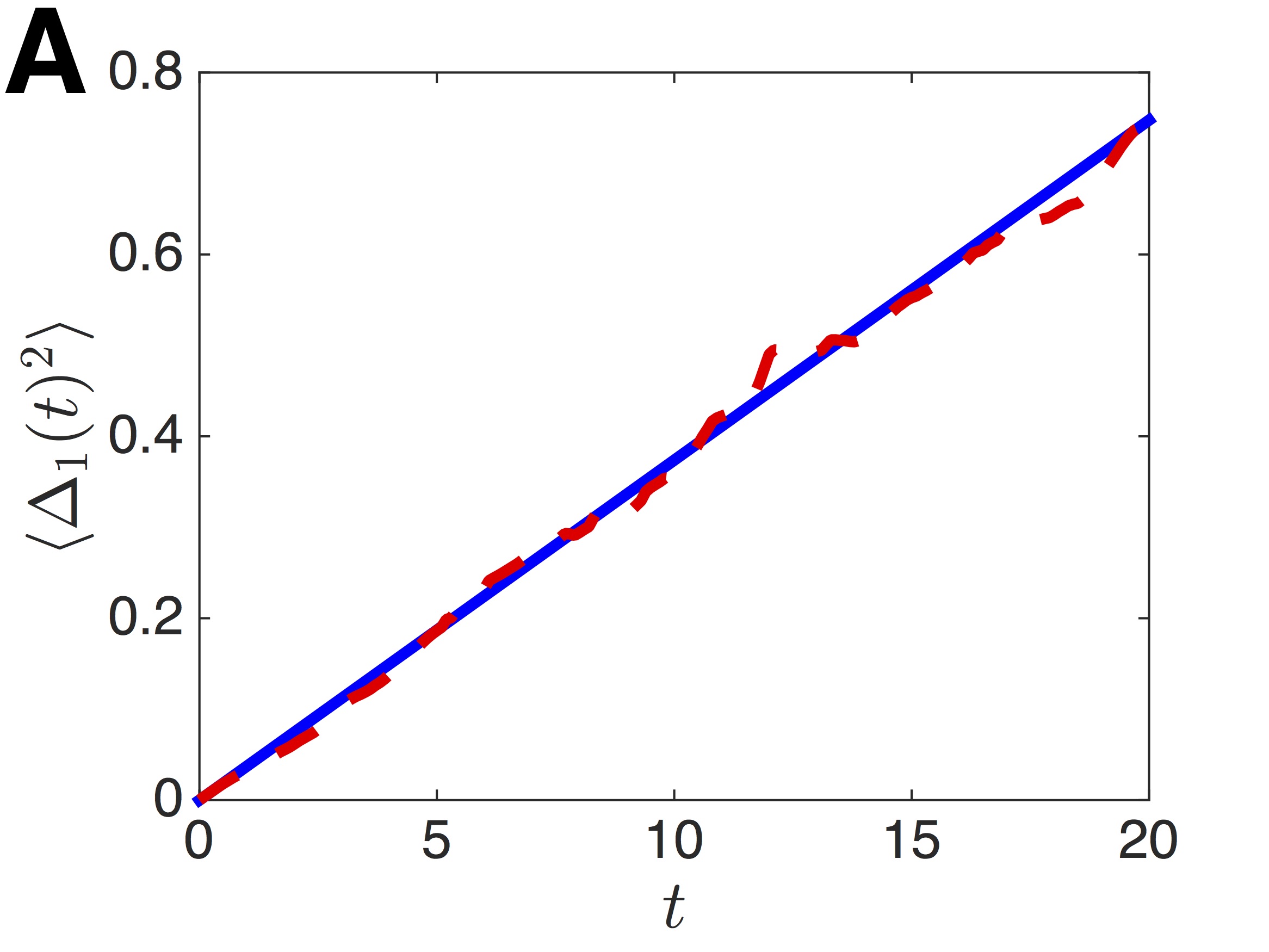
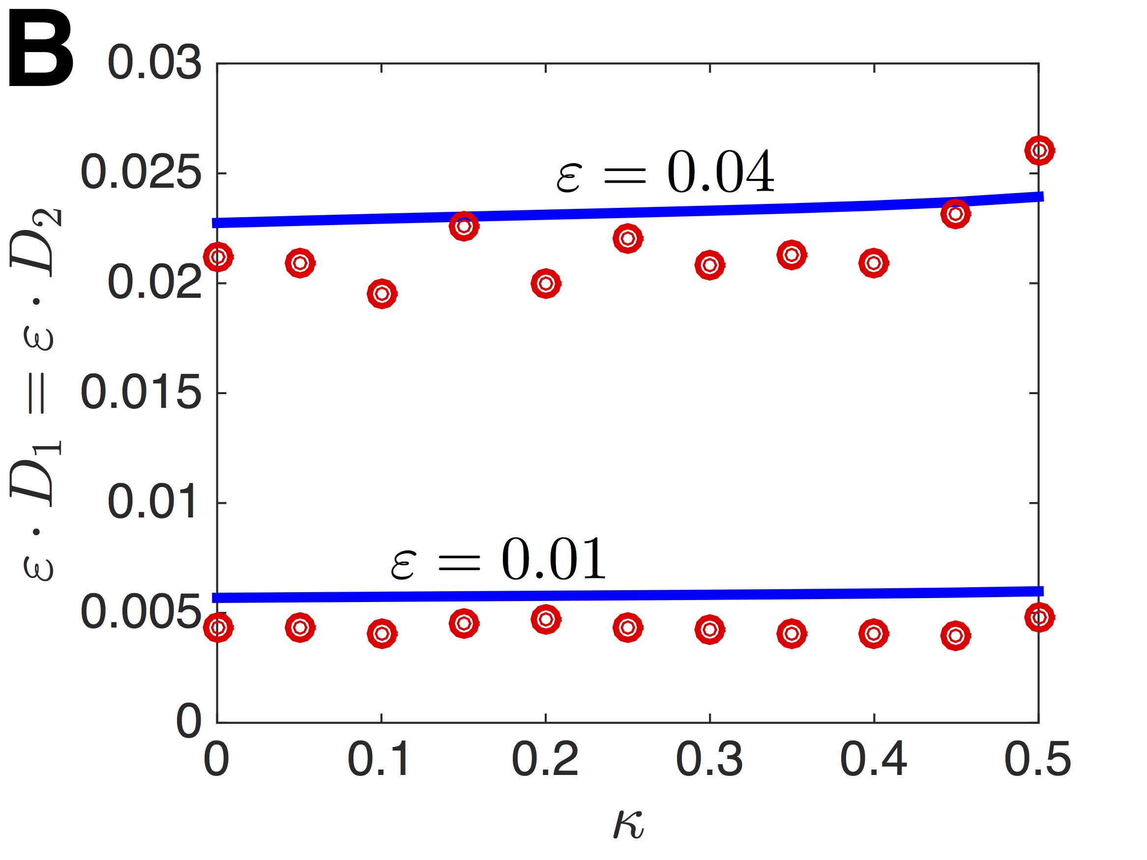
Fig. 3: Variance of the bump position 𝚫(t)=(Δ1(t),Δ2(t))𝚫𝑡subscriptΔ1𝑡subscriptΔ2𝑡{\bm{\Delta}}(t)=(\Delta_{1}(t),\Delta_{2}(t)) evolving according to the stochastic model (5) with Heaviside firing rate (4) and Bessel function weight (2). (A) Long-term variance Δ12\langle\Delta_{1}^{2}\rangle\rangle scales linearly as pure diffusion, and the slope is given by the diffusion coefficient D𝐷D defined by the formula (43). Parameters are κ=0.2𝜅0.2\kappa=0.2 and ε=0.05𝜀0.05\varepsilon=0.05. (B) Plot of the effective diffusion coefficient εD𝜀𝐷\varepsilon\cdot D versus the activity threshold κ𝜅\kappa. The weight function w𝑤w is (19) with [c1,c2,c3,c4]=[5/3,5/3,1/2,1/2]subscript𝑐1subscript𝑐2subscript𝑐3subscript𝑐453531212[c_{1},c_{2},c_{3},c_{4}]=[5/3,-5/3,-1/2,1/2]. Numerical variances are computed using 1000 realizations each.

3.3 Explicit results for the Heaviside firing rate

We now show that we can explicitly calculate the effective diffusion coefficient (41) in the case of a Heaviside firing rate function (4), weight kernel comprised of modified Bessel functions (2), and the following cosine noise correlation function derived in (9):

C(𝐱)=cos(x1)+cos(x2).𝐶𝐱subscript𝑥1subscript𝑥2C({\mathbf{x}})=\cos(x_{1})+\cos(x_{2}). (42)

Analogous to our linear stability calculations, by selecting a Heaviside firing rate function (4), we find that the associated functional derivative f(U)superscript𝑓𝑈f^{\prime}(U) is given by (29). Thus, the domain of integration of the terms in (41) collapse from 2superscript2{\mathbb{R}}^{2} to the closed curve r=a𝑟𝑎r=a, in polar coordinates 𝐫=(r,θ)𝐫𝑟𝜃{\mathbf{r}}=(r,\theta). Furthermore, the spatial derivatives Ux1subscript𝑈subscript𝑥1U_{x_{1}} and Ux2subscript𝑈subscript𝑥2U_{x_{2}} are given by the formulas (27), so that we can simply rewrite the term in the denominator of (41) as an integral over the angular coordinate θ𝜃\theta

(2f(U(𝐱))Uxj2(𝐱)𝑑𝐱)2=superscriptsubscriptsuperscript2superscript𝑓𝑈𝐱superscriptsubscript𝑈subscript𝑥𝑗2𝐱differential-d𝐱2absent\displaystyle\left(\int_{{\mathbb{R}}^{2}}f^{\prime}(U({\mathbf{x}}))U_{x_{j}}^{2}({\mathbf{x}})d{\mathbf{x}}\right)^{2}= (1|U(a)|02π0δ(ra)[U(a)cosθ]2r𝑑r𝑑θ)2superscript1superscript𝑈𝑎superscriptsubscript02𝜋superscriptsubscript0𝛿𝑟𝑎superscriptdelimited-[]superscript𝑈𝑎𝜃2𝑟differential-d𝑟differential-d𝜃2\displaystyle\left(\frac{1}{|U^{\prime}(a)|}\int_{0}^{2\pi}\int_{0}^{\infty}\delta(r-a)\left[U^{\prime}(a)\cos\theta\right]^{2}rdrd\theta\right)^{2}
=\displaystyle= (a|U(a)|02π[U(a)cosθ]2𝑑θ)2=a2π2U(a)2.superscript𝑎superscript𝑈𝑎superscriptsubscript02𝜋superscriptdelimited-[]superscript𝑈𝑎𝜃2differential-d𝜃2superscript𝑎2superscript𝜋2superscript𝑈superscript𝑎2\displaystyle\left(\frac{a}{|U^{\prime}(a)|}\int_{0}^{2\pi}\left[U^{\prime}(a)\cos\theta\right]^{2}d\theta\right)^{2}=a^{2}\pi^{2}U^{\prime}(a)^{2}.

We can apply a similar approach to the calculation of the numerator of (41), given by

a2π2U(a)2Djsuperscript𝑎2superscript𝜋2superscript𝑈superscript𝑎2subscript𝐷𝑗\displaystyle a^{2}\pi^{2}U^{\prime}(a)^{2}D_{j} =22f(U(𝐱))Uxj(𝐱)f(U(𝐲))Uxj(𝐲)C(𝐱𝐲)𝑑𝐲𝑑𝐱absentsubscriptsuperscript2subscriptsuperscript2superscript𝑓𝑈𝐱subscript𝑈subscript𝑥𝑗𝐱superscript𝑓𝑈𝐲subscript𝑈subscript𝑥𝑗𝐲𝐶𝐱𝐲differential-d𝐲differential-d𝐱\displaystyle=\int_{{\mathbb{R}}^{2}}\int_{{\mathbb{R}}^{2}}f^{\prime}(U({\mathbf{x}}))U_{x_{j}}({\mathbf{x}})f^{\prime}(U({\mathbf{y}}))U_{x_{j}}({\mathbf{y}})C({\mathbf{x}}-{\mathbf{y}})d{\mathbf{y}}d{\mathbf{x}}
=a202π02πcosθcosϕC(a(cosθ,sinθ)Ta(cosϕ,sinϕ)T)𝑑θ𝑑ϕ.absentsuperscript𝑎2superscriptsubscript02𝜋superscriptsubscript02𝜋𝜃italic-ϕ𝐶𝑎superscript𝜃𝜃𝑇𝑎superscriptitalic-ϕitalic-ϕ𝑇differential-d𝜃differential-ditalic-ϕ\displaystyle=a^{2}\int_{0}^{2\pi}\int_{0}^{2\pi}\cos\theta\cos\phi\ C(a(\cos\theta,\sin\theta)^{T}-a(\cos\phi,\sin\phi)^{T})d\theta d\phi.

Rewriting by using the cosine correlation function (42) and utilizing the identity cos(xy)=cosxcosy+sinxsiny𝑥𝑦𝑥𝑦𝑥𝑦\cos(x-y)=\cos x\cos y+\sin x\sin y, we have

π2U(a)2Dj=superscript𝜋2superscript𝑈superscript𝑎2subscript𝐷𝑗absent\displaystyle\pi^{2}U^{\prime}(a)^{2}D_{j}= (02πcos(acosθ)cosθdθ)2+(02πcos(asinθ)cosθdθ)2superscriptsuperscriptsubscript02𝜋𝑎𝜃𝜃𝑑𝜃2superscriptsuperscriptsubscript02𝜋𝑎𝜃𝜃𝑑𝜃2\displaystyle\left(\int_{0}^{2\pi}\cos(a\cos\theta)\cos\theta d\theta\right)^{2}+\left(\int_{0}^{2\pi}\cos(a\sin\theta)\cos\theta d\theta\right)^{2}
+(02πsin(acosθ)cosθdθ)2+(02πsin(asinθ)cosθdθ)2.superscriptsuperscriptsubscript02𝜋𝑎𝜃𝜃𝑑𝜃2superscriptsuperscriptsubscript02𝜋𝑎𝜃𝜃𝑑𝜃2\displaystyle+\left(\int_{0}^{2\pi}\sin(a\cos\theta)\cos\theta d\theta\right)^{2}+\left(\int_{0}^{2\pi}\sin(a\sin\theta)\cos\theta d\theta\right)^{2}.

Applying the substitution v=asinθ𝑣𝑎𝜃v=a\sin\theta, we find that

02πcos(asinθ)cosθdθ=1aaacosvdv+1aaacosvdv=superscriptsubscript02𝜋𝑎𝜃𝜃𝑑𝜃1𝑎superscriptsubscript𝑎𝑎𝑣𝑑𝑣1𝑎superscriptsubscript𝑎𝑎𝑣𝑑𝑣absent\displaystyle\int_{0}^{2\pi}\cos(a\sin\theta)\cos\theta d\theta=\frac{1}{a}\int_{-a}^{a}\cos vdv+\frac{1}{a}\int_{a}^{-a}\cos vdv= 0,0\displaystyle\ 0,
02πsin(asinθ)cosθdθ=1aaasinvdv+1aaasinvdv=superscriptsubscript02𝜋𝑎𝜃𝜃𝑑𝜃1𝑎superscriptsubscript𝑎𝑎𝑣𝑑𝑣1𝑎superscriptsubscript𝑎𝑎𝑣𝑑𝑣absent\displaystyle\int_{0}^{2\pi}\sin(a\sin\theta)\cos\theta d\theta=\frac{1}{a}\int_{-a}^{a}\sin vdv+\frac{1}{a}\int_{a}^{-a}\sin vdv= 0.0\displaystyle\ 0.

Furthermore, breaking up the domain of integration of the first summand, we find

02πcos(acosθ)cosθdθ=superscriptsubscript02𝜋𝑎𝜃𝜃𝑑𝜃absent\displaystyle\int_{0}^{2\pi}\cos(a\cos\theta)\cos\theta d\theta= π/2π/2cos(acosθ)cosθdθ+π/23π/2cos(acosθ)cosθdθsuperscriptsubscript𝜋2𝜋2𝑎𝜃𝜃𝑑𝜃superscriptsubscript𝜋23𝜋2𝑎𝜃𝜃𝑑𝜃\displaystyle\int_{-\pi/2}^{\pi/2}\cos(a\cos\theta)\cos\theta d\theta+\int_{\pi/2}^{3\pi/2}\cos(a\cos\theta)\cos\theta d\theta
=\displaystyle= π/2π/2cos(acosθ)cosθdθ+π/2π/2cos(acos(θ+π))cos(θ+π)𝑑θsuperscriptsubscript𝜋2𝜋2𝑎𝜃𝜃𝑑𝜃superscriptsubscript𝜋2𝜋2𝑎𝜃𝜋𝜃𝜋differential-d𝜃\displaystyle\int_{-\pi/2}^{\pi/2}\cos(a\cos\theta)\cos\theta d\theta+\int_{-\pi/2}^{\pi/2}\cos(a\cos(\theta+\pi))\cos(\theta+\pi)d\theta
=\displaystyle= π/2π/2cos(acosθ)cosθdθπ/2π/2cos(acosθ)cosθdθ=0.superscriptsubscript𝜋2𝜋2𝑎𝜃𝜃𝑑𝜃superscriptsubscript𝜋2𝜋2𝑎𝜃𝜃𝑑𝜃0\displaystyle\int_{-\pi/2}^{\pi/2}\cos(a\cos\theta)\cos\theta d\theta-\int_{-\pi/2}^{\pi/2}\cos(a\cos\theta)\cos\theta d\theta=0.

Lastly, we must compute the remaining summand, for which we make use of integration by parts

02πsin(cosθ)cosθdθ=2a0πsin2θcos(acosθ)𝑑θ=2πJ1(a),superscriptsubscript02𝜋𝜃𝜃𝑑𝜃2𝑎superscriptsubscript0𝜋superscript2𝜃𝑎𝜃differential-d𝜃2𝜋subscript𝐽1𝑎\displaystyle\int_{0}^{2\pi}\sin(\cos\theta)\cos\theta d\theta=2a\int_{0}^{\pi}\sin^{2}\theta\cos(a\cos\theta)d\theta=2\pi J_{1}(a),

where we have made use of the explicit integral representation of a Bessel function of the first kind of order ν𝜈\nu:

Jν(z)=1πzν(2ν1)!!0πsin2νθcos(zcosθ)𝑑θ.subscript𝐽𝜈𝑧1𝜋superscript𝑧𝜈double-factorial2𝜈1superscriptsubscript0𝜋superscript2𝜈𝜃𝑧𝜃differential-d𝜃\displaystyle J_{\nu}(z)=\frac{1}{\pi}\frac{z^{\nu}}{(2\nu-1)!!}\int_{0}^{\pi}\sin^{2\nu}\theta\cos(z\cos\theta)d\theta.

Thus, we can finally write

Dj=4J1(a)2U(a)2,j=1,2.formulae-sequencesubscript𝐷𝑗4subscript𝐽1superscript𝑎2superscript𝑈superscript𝑎2𝑗12\displaystyle D_{j}=\frac{4J_{1}(a)^{2}}{U^{\prime}(a)^{2}},\ \ \ \ j=1,2. (43)

Effective diffusion along both the x1subscript𝑥1x_{1} and x2subscript𝑥2x_{2} axes is identical, due to radial symmetry of the bump along with the D4subscript𝐷4D_{4} symmetry of the correlation function (42). We demonstrate our analytical results, in comparison to statistics from numerical simulations, in Fig. 3.

4 Stimulus-pinned bumps in 2superscript2{\mathbb{R}}^{2}

In this section, we explore how the interaction of external inputs and noise determines the stochastic dynamics of bumps. In previous work, we have shown in one-dimensional domains that both external inputs [36] and coupling between bumps in multiple layers [33, 34, 12] can help stabilize bumps to the translating perturbations of noise. Inputs pin bumps in place so their motion is mostly restricted to the peak(s) of the input function, and the stochastic variable describing the bump’s location can be approximated with a mean-reverting (Ornstein-Uhlenbeck) process. Thus, we consider an external stationary stimulus I(𝐱)𝐼𝐱I({\mathbf{x}}) acting on our stochastic system (5), and our modified model takes the form

du(𝐱,t)=(u(𝐱,t)+2w(𝐱𝐲)f(u(𝐱,t))𝑑𝐲+I(𝐱))dt+ε1/2dW(𝐱,t).𝑑𝑢𝐱𝑡𝑢𝐱𝑡subscriptsuperscript2𝑤𝐱𝐲𝑓𝑢𝐱𝑡differential-d𝐲𝐼𝐱𝑑𝑡superscript𝜀12𝑑𝑊𝐱𝑡du({\mathbf{x}},t)=\left(-u({\mathbf{x}},t)+\int_{{\mathbb{R}}^{2}}w({\mathbf{x}}-{\mathbf{y}})f(u({\mathbf{x}},t))\;d{\mathbf{y}}+I({\mathbf{x}})\right)dt+\varepsilon^{1/2}dW({\mathbf{x}},t). (44)

The primary forms of input we employ are a radially symmetric Gaussian

I(𝐱)=I(r)=A0er2/σ2,𝐼𝐱𝐼𝑟subscript𝐴0superscriptesuperscript𝑟2superscript𝜎2\displaystyle I({\mathbf{x}})=I(r)=A_{0}{\rm e}^{-r^{2}/\sigma^{2}}, (45)

and a translationally symmetric Gaussian

I(𝐱)=I(x1)=A0ex12/σ2,𝐼𝐱𝐼subscript𝑥1subscript𝐴0superscriptesuperscriptsubscript𝑥12superscript𝜎2\displaystyle I({\mathbf{x}})=I(x_{1})=A_{0}{\rm e}^{-x_{1}^{2}/\sigma^{2}}, (46)

where I(x1)𝐼subscript𝑥1I(x_{1}) denotes independence from the second coordinate of the spatial vector 𝐱=(x1,x2)𝐱subscript𝑥1subscript𝑥2{\mathbf{x}}=(x_{1},x_{2}). We begin by reviewing the existence and stability of radially symmetric bumps in the noise free system (ε0𝜀0\varepsilon\to 0), as this foreshadows the impact of inputs on the stochastic dynamics of bumps. Essentially, the local stability of bumps to translating perturbations is altered by the input’s spatial heterogeneity.

4.1 Existence and stability of bumps

We begin by constructing the modified equations for radially symmetric bump solutions u(𝐱,t)=U(𝐱)=U(r)𝑢𝐱𝑡𝑈𝐱𝑈𝑟u({\mathbf{x}},t)=U({\mathbf{x}})=U(r) to the model (44) in the absence of noise (ε0𝜀0\varepsilon\to 0). Previous work has shown that inputs can stabilize stationary bumps in purely excitatory neural field models that incorporate linear adaptation [23] by altering the evolution of expanding/contracting (O(2)𝑂2O(2)-symmetric) perturbations to bump profiles. Here, we show inputs stabilize bumps to translating (D1subscript𝐷1D_{1}-symmetric) perturbations. We focus on the case where the external input I(𝐱)𝐼𝐱I({\mathbf{x}}) is rotationally symmetric, so in polar coordinates, I(r,θ)=I(r,θ+s)𝐼𝑟𝜃𝐼𝑟𝜃𝑠I(r,\theta)=I(r,\theta+s) for s[0,2π]𝑠02𝜋s\in[0,2\pi]. Thus, our stationary bump solution satisfies the stationary equation

U(𝐱)=2w(𝐱𝐲)f(U(𝐲))𝑑𝐲+I(𝐱),𝑈norm𝐱subscriptsuperscript2𝑤𝐱𝐲𝑓𝑈𝐲differential-d𝐲𝐼𝐱U(||{\mathbf{x}}||)=\int_{{\mathbb{R}}^{2}}w({\mathbf{x}}-{\mathbf{y}})f(U({\mathbf{y}}))d{\mathbf{y}}+I({\mathbf{x}}), (47)

and by changing to polar coordinates 𝐱=(x1,x2)(r,θ)𝐱subscript𝑥1subscript𝑥2maps-to𝑟𝜃{\mathbf{x}}=(x_{1},x_{2})\mapsto(r,\theta), we have

U(r)=02π0w(|𝐫𝐫|)f(U(𝐫))r𝑑r𝑑θ+I(r).𝑈𝑟superscriptsubscript02𝜋superscriptsubscript0𝑤𝐫superscript𝐫𝑓𝑈superscript𝐫superscript𝑟differential-dsuperscript𝑟differential-dsuperscript𝜃𝐼𝑟\displaystyle U(r)=\int_{0}^{2\pi}\int_{0}^{\infty}w(|{\mathbf{r}}-{\mathbf{r}}^{\prime}|)f(U({\mathbf{r}}^{\prime}))r^{\prime}dr^{\prime}d\theta^{\prime}+I(r). (48)

Assuming a Heaviside firing rate function (4), the integral in (48) collapses to a compact domain

U(r)=02π0aw(|𝐫𝐫|)r𝑑r𝑑θ+I(r),𝑈𝑟superscriptsubscript02𝜋superscriptsubscript0𝑎𝑤𝐫superscript𝐫superscript𝑟differential-dsuperscript𝑟differential-dsuperscript𝜃𝐼𝑟\displaystyle U(r)=\int_{0}^{2\pi}\int_{0}^{a}w(|{\mathbf{r}}-{\mathbf{r}}^{\prime}|)r^{\prime}dr^{\prime}d\theta^{\prime}+I(r), (49)

where ra𝑟𝑎r\equiv a defines the boundary bump as in the input-free case (12). We can evaluate (49) explicitly by assuming the weight function formula is a sum of modified Bessel functions (2), finding

U(r)=2πaj=1Nck(a,r,αk)+I(r),𝑈𝑟2𝜋𝑎superscriptsubscript𝑗1𝑁subscript𝑐𝑘𝑎𝑟subscript𝛼𝑘𝐼𝑟\displaystyle U(r)=2\pi a\sum_{j=1}^{N}c_{k}{\mathcal{I}}(a,r,\alpha_{k})+I(r),

where (a,r,s)𝑎𝑟𝑠{\mathcal{I}}(a,r,s) is defined by the formula (17). To relate the bump radius a𝑎a to the threshold κ𝜅\kappa of the Heaviside firing rate function (4), we apply the condition U(a)=κ𝑈𝑎𝜅U(a)=\kappa, which can be written

U(a)=2πaj=1NckαkI1(αka)K0(αka)+I(a)=κ.𝑈𝑎2𝜋𝑎superscriptsubscript𝑗1𝑁subscript𝑐𝑘subscript𝛼𝑘subscript𝐼1subscript𝛼𝑘𝑎subscript𝐾0subscript𝛼𝑘𝑎𝐼𝑎𝜅\displaystyle U(a)=2\pi a\sum_{j=1}^{N}\frac{c_{k}}{\alpha_{k}}I_{1}(\alpha_{k}a)K_{0}(\alpha_{k}a)+I(a)=\kappa.

One can then solve this nonlinear equation using numerical root finding.

To determine the stability of the input-driven stationary bump solution (48), we study the impact of small smooth pertubations by employing the ansatz u(𝐱,t)=U(𝐱)+εΨ(𝐱,t)𝑢𝐱𝑡𝑈𝐱𝜀Ψ𝐱𝑡u({\mathbf{x}},t)=U({\mathbf{x}})+\varepsilon\Psi({\mathbf{x}},t) where ε1much-less-than𝜀1\varepsilon\ll 1. Substituting this expansion into (44), when W0𝑊0W\equiv 0, and truncating to linear order yields the equation (20) as in the input-free case. The main difference is that bumps are defined by (48), incorporating the input term I(𝐱)𝐼𝐱I({\mathbf{x}}). Furthermore, applying separation of variables Ψ(𝐱,t)=Ψ(𝐱)eλtΨ𝐱𝑡Ψ𝐱superscripte𝜆𝑡\Psi({\mathbf{x}},t)=\Psi({\mathbf{x}}){\rm e}^{\lambda t} and rearranging terms yields the eigenvalue equation (21). However, when U(𝐱)𝑈𝐱U({\mathbf{x}}) satisfies (48), such bumps are no longer neutrally stable to perturbations that shift their position. It is straightforward to show this in the case of a Heaviside firing rate function (4), in which case eigenvalues associated with the Fourier modes Ψn(θ)=einθsubscriptΨ𝑛𝜃superscripte𝑖𝑛𝜃\Psi_{n}(\theta)={\rm e}^{in\theta} are given by the expression (31), so the eigenvalue λ1subscript𝜆1\lambda_{1} associated with shifts perturbations Ψ1(θ)=eiθsubscriptΨ1𝜃superscripte𝑖𝜃\Psi_{1}(\theta)={\rm e}^{i\theta} is given by the formula

λ1=1+a|U(a)|02πw(2asin(θ/2))cos(θ)𝑑θ,subscript𝜆11𝑎superscript𝑈𝑎superscriptsubscript02𝜋𝑤2𝑎𝜃2𝜃differential-d𝜃\displaystyle\lambda_{1}=-1+\frac{a}{|U^{\prime}(a)|}\int_{0}^{2\pi}w(2a\sin(\theta/2))\cos(\theta)d\theta, (50)

and since U(r)𝑈𝑟U(r) is given by (49), then

|U(a)|=a02πw(2asin(θ/2))cos(θ)𝑑θI(a).superscript𝑈𝑎𝑎superscriptsubscript02𝜋𝑤2𝑎𝜃2𝜃differential-d𝜃superscript𝐼𝑎\displaystyle|U^{\prime}(a)|=a\int_{0}^{2\pi}w(2a\sin(\theta/2))\cos(\theta)d\theta-I^{\prime}(a).

Thus, we can rewrite (50) as

λ1=I(a)a02πw(2asin(θ/2))cos(θ)𝑑θI(a)<0,subscript𝜆1superscript𝐼𝑎𝑎superscriptsubscript02𝜋𝑤2𝑎𝜃2𝜃differential-d𝜃superscript𝐼𝑎0\displaystyle\lambda_{1}=\frac{I^{\prime}(a)}{a\int_{0}^{2\pi}w(2a\sin(\theta/2))\cos(\theta)d\theta-I^{\prime}(a)}<0,

where the inequality holds when I(r)𝐼𝑟I(r) is a monotone decreasing function, as we have assumed for the radially symmetric Gaussian (45). This indicates the bump will be linearly stable to perturbations that alter its position, indicative of the mean-reverting stochastic dynamics that emerge when weak noise is considered in (44). Eigenvalues of all Fourier modes, representing azimuthal perturbations of the bump (49), can be computed numerically from the formula (31).
Refer to caption
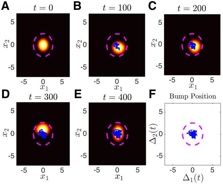
Fig. 4: Numerical simulation of the stochastic neural field (44) on the plane 2superscript2{\mathbb{R}}^{2} with Heaviside firing rate (4) and Bessel function weight (2), subject to radially symmetric Gaussian input (45). Thin lines represents the stochastic trajectory of the bump during the time between the previous and current snapshot. Dashed circle is a plot of the level set I(𝐱)=κ𝐼𝐱𝜅I({\mathbf{x}})=\kappa. (A-E) Snapshots of a simulation of a bump wandering on the plane, due to noise with spatial correlation function C(𝐱)=cos(𝐱)𝐶𝐱𝐱C({\mathbf{x}})=\cos({\mathbf{x}}), at time points t=0,100,200,300,400𝑡0100200300400t=0,100,200,300,400. Input causes the trajectory to stay in the vicinity of the peak of the radially symmetric Gaussian (45) at the origin (x1,x2)=(0,0)subscript𝑥1subscript𝑥200(x_{1},x_{2})=(0,0). (F) Plot of the trajectory of the bump centroid for t[0,400]𝑡0400t\in[0,400] demonstrates how its stochastic trajectory behaves as 2D OU process. Parameters are ε=0.04𝜀0.04\varepsilon=0.04, κ=0.2𝜅0.2\kappa=0.2, A0=1subscript𝐴01A_{0}=1, σ=2𝜎2\sigma=2, and w𝑤w is (19) with [c1,c2,c3,c4]=[5/3,5/3,1/2,1/2]subscript𝑐1subscript𝑐2subscript𝑐3subscript𝑐453531212[c_{1},c_{2},c_{3},c_{4}]=[5/3,-5/3,-1/2,1/2].
Refer to caption
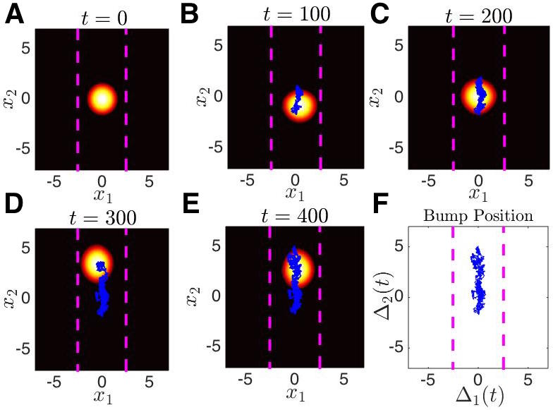
Fig. 5: Numerical simulation of the stochastic neural field (44) on the plane 2superscript2{\mathbb{R}}^{2} with Heaviside firing rate (4) and Bessel function weight (2), subject to translationally symmetric Gaussian input (46). Thin lines represents the stochastic trajectory of the bump during the time between the previous and current snapshot. Dashed lines ar a plot of the level set I(𝐱)=κ𝐼𝐱𝜅I({\mathbf{x}})=\kappa. (A-E) Snapshots of a simulation of a bump wandering on the plane, due to noise with spatial correlation function C(𝐱)=cos(𝐱)𝐶𝐱𝐱C({\mathbf{x}})=\cos({\mathbf{x}}), at time points t=0,100,200,300,400𝑡0100200300400t=0,100,200,300,400. Input cause the trajectory to stay in the vicinity of the peak of the translationally symmetric Gaussian (46) along the line x1=0subscript𝑥10x_{1}=0. (F) Plot of the trajectory of the bump centroid for t[0,400]𝑡0400t\in[0,400] demonstrates how its stochastic trajectory behaves as 2D OU process. Parameters are ε=0.04𝜀0.04\varepsilon=0.04, κ=0.2𝜅0.2\kappa=0.2, A0=1subscript𝐴01A_{0}=1, σ=2𝜎2\sigma=2, and w𝑤w is (19) with [c1,c2,c3,c4]=[5/3,5/3,1/2,1/2]subscript𝑐1subscript𝑐2subscript𝑐3subscript𝑐453531212[c_{1},c_{2},c_{3},c_{4}]=[5/3,-5/3,-1/2,1/2].

4.2 Stochastic bump motion in the presence of weak inputs

Our analysis of the stochastic motion of bumps in the stationary input-driven system (44) employs a similar approach to our analysis of the input-free (I(𝐱)0𝐼𝐱0I({\mathbf{x}})\equiv 0) system (5). However, the effective equations that emerge are no longer translationally invariant, now depending on the spatial heterogeneity imposed by the input I(𝐱)𝐼𝐱I({\mathbf{x}}). Our analysis assumes that inputs are weak, having the same amplitude as the noise term [12], so we write I(𝐱)=ε1/2I~(𝐱)𝐼𝐱superscript𝜀12~𝐼𝐱I({\mathbf{x}})=\varepsilon^{1/2}\tilde{I}({\mathbf{x}}). In this case, the 𝒪(1)𝒪1{\mathcal{O}}(1) terms are identical to the input-free deterministic system (1) with stationary bump solution (10). We can then derive a system of nonlinear stochastic differential equations for the effective motion of the bump’s position 𝚫(t)=(Δ1(t),Δ2(t))𝚫𝑡subscriptΔ1𝑡subscriptΔ2𝑡{\bm{\Delta}}(t)=(\Delta_{1}(t),\Delta_{2}(t)), which we can then truncate to a multivariate Ornstein-Uhlenbeck (OU) process assuming 𝚫(t)𝚫𝑡{\bm{\Delta}}(t) remains small. This captures the fact that bumps are systematically drawn back to the location of the peak(s) of the external input as demonstrated in Fig. 4 and Fig. 5.

Employing the ansatz (33), assuming the bump’s profile has fluctuations ε1/2Φ(𝐱,t)superscript𝜀12Φ𝐱𝑡\varepsilon^{1/2}\Phi({\mathbf{x}},t) on fast timescales and stochastically varying position 𝚫(t)𝚫𝑡{\bm{\Delta}}(t) on longer timescales, we truncate to linear order in ε1/2superscript𝜀12\varepsilon^{1/2} and find

dΦ(𝐱,t)=Φ(𝐱,t)+ε1/2U(𝐱)d𝚫(t)+dW(𝐱,t)+I~(𝐱+𝚫(t)),𝑑Φ𝐱𝑡Φ𝐱𝑡superscript𝜀12𝑈𝐱𝑑𝚫𝑡𝑑𝑊𝐱𝑡~𝐼𝐱𝚫𝑡d\Phi({\mathbf{x}},t)=\mathcal{L}\Phi({\mathbf{x}},t)+\varepsilon^{-1/2}\nabla U({\mathbf{x}})\cdot d\mathbf{\Delta}(t)+dW({\mathbf{x}},t)+\tilde{I}({\mathbf{x}}+\mathbf{\Delta}(t)), (51)

where U(𝐱)=(Ux1(𝐱),Ux2(𝐱))T𝑈𝐱superscriptsubscript𝑈subscript𝑥1𝐱subscript𝑈subscript𝑥2𝐱𝑇\nabla U({\mathbf{x}})=(U_{x_{1}}({\mathbf{x}}),U_{x_{2}}({\mathbf{x}}))^{T} and {\mathcal{L}} is the non-self-adjoint linear operator (35) with adjoint superscript{\mathcal{L}}^{*} given by (36). As before, the nullspace of superscript{\mathcal{L}}^{*} is spanned by the two functions φ1(𝐱)=f(U(𝐱))Ux1(𝐱)subscript𝜑1𝐱superscript𝑓𝑈𝐱subscript𝑈subscript𝑥1𝐱\varphi_{1}({\mathbf{x}})=f^{\prime}(U({\mathbf{x}}))U_{x_{1}}({\mathbf{x}}) and φ2(𝐱)=f(U(𝐱))Ux2(𝐱)subscript𝜑2𝐱superscript𝑓𝑈𝐱subscript𝑈subscript𝑥2𝐱\varphi_{2}({\mathbf{x}})=f^{\prime}(U({\mathbf{x}}))U_{x_{2}}({\mathbf{x}}). Thus, we can enforce solvability of the 𝒪(ε1/2)𝒪superscript𝜀12{\mathcal{O}}(\varepsilon^{1/2}) equation (51) to yield the pair of nonlinear stochastic differential equations

dΔj(t)=ε1/2Gj(𝚫(t))dtε1/2d𝒲j(t),𝑑subscriptΔ𝑗𝑡superscript𝜀12subscript𝐺𝑗𝚫𝑡𝑑𝑡superscript𝜀12𝑑subscript𝒲𝑗𝑡\displaystyle d\Delta_{j}(t)=-\varepsilon^{1/2}G_{j}({\bm{\Delta}}(t))dt-\varepsilon^{1/2}d{\mathcal{W}}_{j}(t), (52)

where the restorative dynamics of the input are described by the nonlinear function

Gj(𝚫)=2f(U(𝐱))Uxj(𝐱)I~(𝐱+𝚫)𝑑𝐱2f(U(𝐱))Uxj2(𝐱)𝑑𝐱,j{1,2},formulae-sequencesubscript𝐺𝑗𝚫subscriptsuperscript2superscript𝑓𝑈𝐱subscript𝑈subscript𝑥𝑗𝐱~𝐼𝐱𝚫differential-d𝐱subscriptsuperscript2superscript𝑓𝑈𝐱superscriptsubscript𝑈subscript𝑥𝑗2𝐱differential-d𝐱𝑗12\displaystyle G_{j}({\bm{\Delta}})=\frac{\int_{{\mathbb{R}}^{2}}f^{\prime}(U({\mathbf{x}}))U_{x_{j}}({\mathbf{x}})\tilde{I}({\mathbf{x}}+{\bm{\Delta}})d{\mathbf{x}}}{\int_{{\mathbb{R}}^{2}}f^{\prime}(U({\mathbf{x}}))U_{x_{j}}^{2}({\mathbf{x}})d{\mathbf{x}}},\ \ \ \ \ j\in\{1,2\}, (53)

and spatiotemporal noise provides the effective noise perturbations to the bump position through the white noise terms

𝒲j(t)=2f(U(𝐱))Uxj(𝐱)W(𝐱,t)𝑑𝐱2f(U(𝐱))Uxj2(𝐱)𝑑𝐱,j{1,2}.formulae-sequencesubscript𝒲𝑗𝑡subscriptsuperscript2superscript𝑓𝑈𝐱subscript𝑈subscript𝑥𝑗𝐱𝑊𝐱𝑡differential-d𝐱subscriptsuperscript2superscript𝑓𝑈𝐱superscriptsubscript𝑈subscript𝑥𝑗2𝐱differential-d𝐱𝑗12\displaystyle{\mathcal{W}}_{j}(t)=\frac{\int_{{\mathbb{R}}^{2}}f^{\prime}(U({\mathbf{x}}))U_{x_{j}}({\mathbf{x}})W({\mathbf{x}},t)d{\mathbf{x}}}{\int_{{\mathbb{R}}^{2}}f^{\prime}(U({\mathbf{x}}))U_{x_{j}}^{2}({\mathbf{x}})d{\mathbf{x}}},\ \ \ \ \ j\in\{1,2\}. (54)

Note that d𝒲j(t)=0delimited-⟨⟩𝑑subscript𝒲𝑗𝑡0\langle d{\mathcal{W}}_{j}(t)\rangle=0 and d𝒲(t)d𝒲(s)=2Djδ(ts)dtdsdelimited-⟨⟩𝑑𝒲𝑡𝑑𝒲𝑠2subscript𝐷𝑗𝛿𝑡𝑠𝑑𝑡𝑑𝑠\langle d{\mathcal{W}}(t)d{\mathcal{W}}(s)\rangle=2D_{j}\delta(t-s)dtds with Djsubscript𝐷𝑗D_{j} given by (41). As we demonstrated in our analysis of stimulus-driven bump existence and stability, 𝚫¯=(0,0)¯𝚫00\bar{{\bm{\Delta}}}=(0,0) is a stable fixed point of the noise-free system Δ˙j(t)=ε1/2Gj(𝚫(t))subscript˙Δ𝑗𝑡superscript𝜀12subscript𝐺𝑗𝚫𝑡\dot{\Delta}_{j}(t)=-\varepsilon^{1/2}G_{j}({\bm{\Delta}}(t)); j=1,2𝑗12j=1,2. Linearizing about this solution yields the multivariate OU process

dΔj(t)+ε1/2βjΔj(t)dt=ε1/2d𝒲j(t),𝑑subscriptΔ𝑗𝑡superscript𝜀12subscript𝛽𝑗subscriptΔ𝑗𝑡𝑑𝑡superscript𝜀12𝑑subscript𝒲𝑗𝑡\displaystyle d\Delta_{j}(t)+\varepsilon^{1/2}\beta_{j}\Delta_{j}(t)dt=\varepsilon^{1/2}d{\mathcal{W}}_{j}(t), (55)

where

βj=G(0)=2f(U(𝐱))Uxj(𝐱)I~xj(𝐱)𝑑𝐱2f(U(𝐱))Uxj2(𝐱)𝑑𝐱,j{1,2},formulae-sequencesubscript𝛽𝑗superscript𝐺0subscriptsuperscript2superscript𝑓𝑈𝐱subscript𝑈subscript𝑥𝑗𝐱subscript~𝐼subscript𝑥𝑗𝐱differential-d𝐱subscriptsuperscript2superscript𝑓𝑈𝐱superscriptsubscript𝑈subscript𝑥𝑗2𝐱differential-d𝐱𝑗12\displaystyle\beta_{j}=G^{\prime}(0)=\frac{\int_{{\mathbb{R}}^{2}}f^{\prime}(U({\mathbf{x}}))U_{x_{j}}({\mathbf{x}})\tilde{I}_{x_{j}}({\mathbf{x}})d{\mathbf{x}}}{\int_{{\mathbb{R}}^{2}}f^{\prime}(U({\mathbf{x}}))U_{x_{j}}^{2}({\mathbf{x}})d{\mathbf{x}}},\ \ \ \ \ j\in\{1,2\}, (56)

assuming 2f(U(𝐱))Uxj(𝐱)I~xk(𝐱)𝑑𝐱0subscriptsuperscript2superscript𝑓𝑈𝐱subscript𝑈subscript𝑥𝑗𝐱subscript~𝐼subscript𝑥𝑘𝐱differential-d𝐱0\int_{{\mathbb{R}}^{2}}f^{\prime}(U({\mathbf{x}}))U_{x_{j}}({\mathbf{x}})\tilde{I}_{x_{k}}({\mathbf{x}})d{\mathbf{x}}\equiv 0, when jk𝑗𝑘j\neq k, which is the case when I(𝐱)𝐼𝐱I({\mathbf{x}}) is even symmetric along the x1subscript𝑥1x_{1} and x2subscript𝑥2x_{2} directions as (45) and (46) are. In this case, we can use standard properties of an OU process to compute the mean Δj(t)=Δj(0)eε1/2βjtdelimited-⟨⟩subscriptΔ𝑗𝑡subscriptΔ𝑗0superscript𝑒superscript𝜀12subscript𝛽𝑗𝑡\langle\Delta_{j}(t)\rangle=\Delta_{j}(0)e^{-\varepsilon^{1/2}\beta_{j}t} and variance

Δj(t)2=ε1/2Djβj(1e2ε1/2βjt),delimited-⟨⟩subscriptΔ𝑗superscript𝑡2superscript𝜀12subscript𝐷𝑗subscript𝛽𝑗1superscript𝑒2superscript𝜀12subscript𝛽𝑗𝑡\displaystyle\langle\Delta_{j}(t)^{2}\rangle=\frac{\varepsilon^{1/2}D_{j}}{\beta_{j}}\left(1-e^{-2\varepsilon^{1/2}\beta_{j}t}\right), (57)

so the variance Δj(t)2delimited-⟨⟩subscriptΔ𝑗superscript𝑡2\langle\Delta_{j}(t)^{2}\rangle will approach a constant ε1/2Dj/βjsuperscript𝜀12subscript𝐷𝑗subscript𝛽𝑗\varepsilon^{1/2}D_{j}/\beta_{j} as t𝑡t\to\infty and the mean converges to the fixed point 𝚫¯=(0,0)¯𝚫00\bar{{\bm{\Delta}}}=(0,0). Thus, we can describe the stochastic dynamics of the position 𝚫(t)𝚫𝑡{\bm{\Delta}}(t) approximately using a multivariate OU process (55) or with higher order corrections through the nonlinear SDE (52).
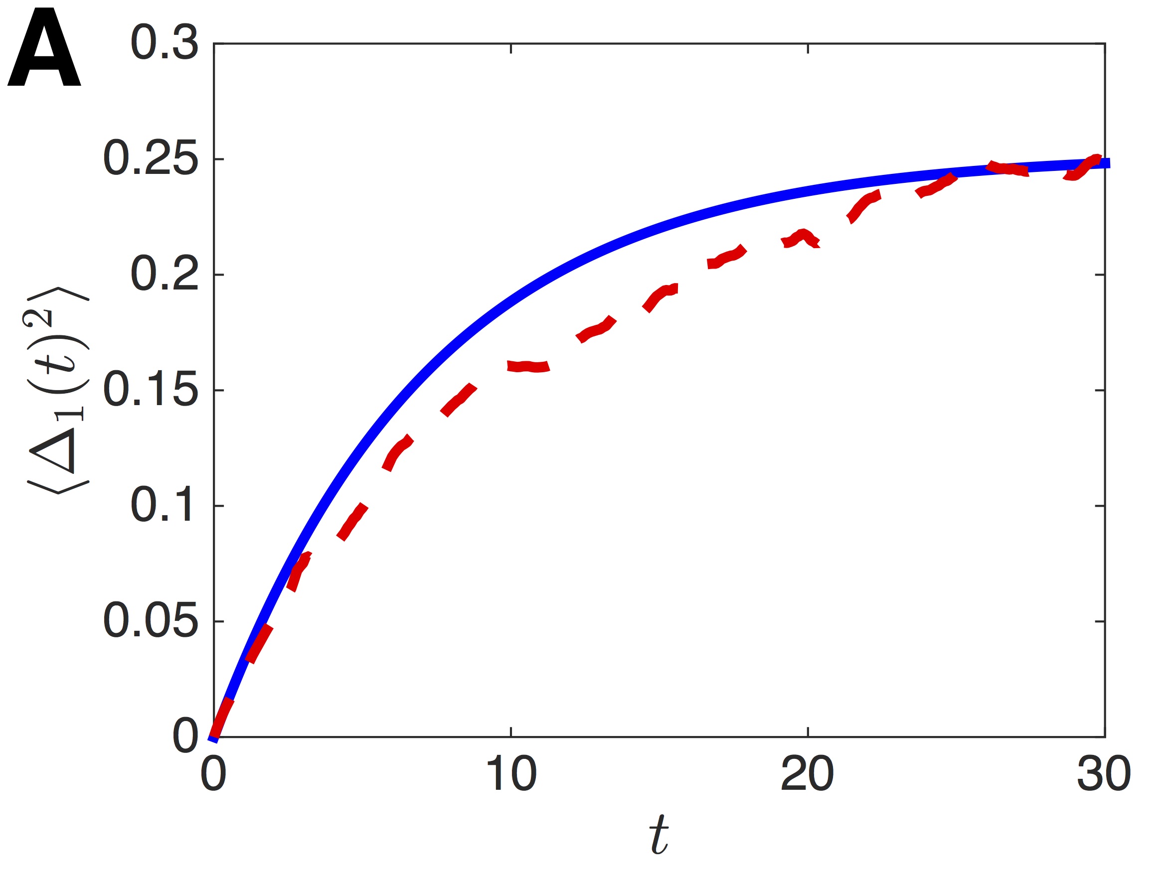
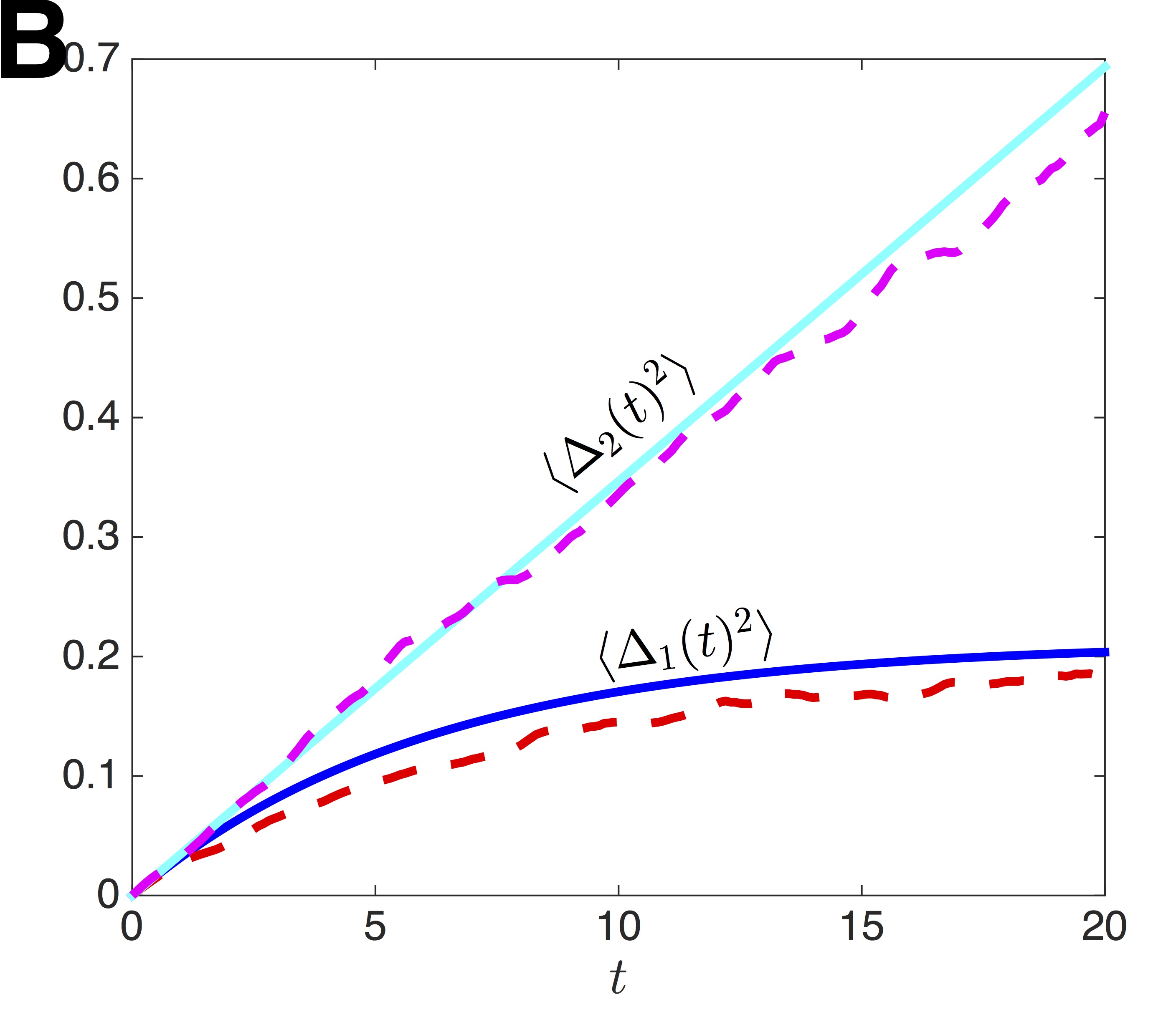
Refer to caption
Refer to caption
Fig. 6: Variance of the bump position 𝚫(t)=(Δ1(t),Δ2(t))𝚫𝑡subscriptΔ1𝑡subscriptΔ2𝑡{\bm{\Delta}}(t)=(\Delta_{1}(t),\Delta_{2}(t)) evolving according to the stochastic model (44) with Heaviside firing rate (4) and Bessel function weight (2). (A) Long-term variance Δ1(t)2delimited-⟨⟩subscriptΔ1superscript𝑡2\langle\Delta_{1}(t)^{2}\rangle saturates according to a multivariate Ornstein-Uhlenbeck process when input is given by a radially symmetric Gaussian (45). Results from numerical simulations (dashed line) are well matched to our theoretical result (57). An identical picture exists for Δ2(t)2delimited-⟨⟩subscriptΔ2superscript𝑡2\langle\Delta_{2}(t)^{2}\rangle, the variance along the x2subscript𝑥2x_{2} direction. (B) Variance along the x2subscript𝑥2x_{2} direction Δ2(t)2delimited-⟨⟩subscriptΔ2superscript𝑡2\langle\Delta_{2}(t)^{2}\rangle climbs linearly and variance Δ1(t)2delimited-⟨⟩subscriptΔ1superscript𝑡2\langle\Delta_{1}(t)^{2}\rangle along the x1subscript𝑥1x_{1} direction saturates when input is given by a translationally symmetric Gaussian (46). Parameters are κ=0.2𝜅0.2\kappa=0.2, A0=1subscript𝐴01A_{0}=1, σ=2𝜎2\sigma=2, and w𝑤w is (19) with [c1,c2,c3,c4]=[5/3,5/3,1/2,1/2]subscript𝑐1subscript𝑐2subscript𝑐3subscript𝑐453531212[c_{1},c_{2},c_{3},c_{4}]=[5/3,-5/3,-1/2,1/2]. Numerical calculations of variance use 1000 realizations each.

4.3 Explicit results for the Heaviside firing rate

We can explicitly calculate the variances Δj(t)2delimited-⟨⟩subscriptΔ𝑗superscript𝑡2\langle\Delta_{j}(t)^{2}\rangle as described by the formula (57) in the case of a Heaviside firing rate function (4), Bessel function weight kernel (2), and cosine noise correlations (42). Thus, the derivative f(U)superscript𝑓𝑈f^{\prime}(U) is given by (29), spatial derivatives Uxjsubscript𝑈subscript𝑥𝑗U_{x_{j}} (j=1,2𝑗12j=1,2) are given by (27), and the diffusion coefficients Djsubscript𝐷𝑗D_{j} (j=1,2𝑗12j=1,2) are defined by the formula (43). Again, the impact of spatiotemporal noise in bump dynamics is primarily determined by interactions that occur at the bump boundary ra𝑟𝑎r\equiv a. Furthermore, in the case of a radially symmetric input such as the Gaussian (45), we can compute the coefficients

βj=2f(U(𝐱))Uxj(𝐱)I~xj(𝐱)𝑑𝐱2f(U(𝐱))Uxj2(𝐱)𝑑𝐱=aπI~(a)aπU(a)=I~(a)U(a),j={1,2}.formulae-sequencesubscript𝛽𝑗subscriptsuperscript2superscript𝑓𝑈𝐱subscript𝑈subscript𝑥𝑗𝐱subscript~𝐼subscript𝑥𝑗𝐱differential-d𝐱subscriptsuperscript2superscript𝑓𝑈𝐱superscriptsubscript𝑈subscript𝑥𝑗2𝐱differential-d𝐱𝑎𝜋superscript~𝐼𝑎𝑎𝜋superscript𝑈𝑎superscript~𝐼𝑎superscript𝑈𝑎𝑗12\displaystyle\beta_{j}=\frac{\int_{{\mathbb{R}}^{2}}f^{\prime}(U({\mathbf{x}}))U_{x_{j}}({\mathbf{x}})\tilde{I}_{x_{j}}({\mathbf{x}})d{\mathbf{x}}}{\int_{{\mathbb{R}}^{2}}f^{\prime}(U({\mathbf{x}}))U_{x_{j}}^{2}({\mathbf{x}})d{\mathbf{x}}}=\frac{a\pi\tilde{I}^{\prime}(a)}{a\pi U^{\prime}(a)}=\frac{\tilde{I}^{\prime}(a)}{U^{\prime}(a)},\ \ \ \ \ j=\{1,2\}. (58)

Therefore, in the long time limit, the variances Δj(t)2delimited-⟨⟩subscriptΔ𝑗superscript𝑡2\langle\Delta_{j}(t)^{2}\rangle will saturate to

limtΔj(t)2=ε1/2Djβj=4εJ1(a)2I(a)U(a).subscript𝑡delimited-⟨⟩subscriptΔ𝑗superscript𝑡2superscript𝜀12subscript𝐷𝑗subscript𝛽𝑗4𝜀subscript𝐽1superscript𝑎2superscript𝐼𝑎superscript𝑈𝑎\displaystyle\lim_{t\to\infty}\langle\Delta_{j}(t)^{2}\rangle=\frac{\varepsilon^{1/2}D_{j}}{\beta_{j}}=\frac{4\varepsilon J_{1}(a)^{2}}{I^{\prime}(a)U^{\prime}(a)}. (59)

We compare our explicit calculation of the variance to results from numerical calculations for the case of a radially symmetric Gaussian (45) in Fig. 6A.

In the case of the translationally symmetric Gaussian (46), we have that Ix2(𝐱)0subscript𝐼subscript𝑥2𝐱0I_{x_{2}}({\mathbf{x}})\equiv 0, so β20subscript𝛽20\beta_{2}\equiv 0. As a result Δ2(t)2=εD2tdelimited-⟨⟩subscriptΔ2superscript𝑡2𝜀subscript𝐷2𝑡\langle\Delta_{2}(t)^{2}\rangle=\varepsilon D_{2}t, and the variance is only mean reverting along the x1subscript𝑥1x_{1} direction, as demonstrated by the numerical simulation in Fig. 5. The coefficient describing the systematic dynamics along the x1subscript𝑥1x_{1} direction is

ε1/2β1=2aA002πexp[a2cos2θ/σ2]cos2θdθπσ2|U(a)|,superscript𝜀12subscript𝛽12𝑎subscript𝐴0superscriptsubscript02𝜋expdelimited-[]superscript𝑎2superscript2𝜃superscript𝜎2superscript2𝜃𝑑𝜃𝜋superscript𝜎2superscript𝑈𝑎\displaystyle\varepsilon^{1/2}\beta_{1}=\frac{2aA_{0}\int_{0}^{2\pi}{\rm exp}\left[\displaystyle-a^{2}\cos^{2}\theta/\sigma^{2}\right]\cos^{2}\theta d\theta}{\pi\sigma^{2}|U^{\prime}(a)|}, (60)

which can be computed using quadrature to evaluate the formula (57) for j=1𝑗1j=1. We compare these theoretical results with averages across numerical realizations in Fig. 6B. Thus, the variance along the x1subscript𝑥1x_{1}-direction saturates, while the variance along the x2subscript𝑥2x_{2}-direction indefinitely climbs linearly.

4.4 Statistics of the nonlinear Langevin equation

More accurate approximations of the variances Δj2delimited-⟨⟩superscriptsubscriptΔ𝑗2\langle\Delta_{j}^{2}\rangle can be obtained by performing an analysis of the full nonlinear Langevin equation (52) for the stochastic motion of the input-driven bump. In [12], it was recently shown this can be particularly useful when there are multiple distinct fixed points of the noise free equations Δ˙j=ε1/2Gj(Δ)subscript˙Δ𝑗superscript𝜀12subscript𝐺𝑗Δ\dot{\Delta}_{j}=-\varepsilon^{1/2}G_{j}(\Delta) (j=1,2𝑗12j=1,2), as noise can eventually cause a phase-slip so a linearized approximation is no longer valid. Here, we demonstrate that a derivation of nonlinear Langevin equations can be extended to spatiotemporal patterns evolving in two-dimensions. Also, even if the position 𝚫(t)=(Δ1(t),Δ2(t))𝚫𝑡subscriptΔ1𝑡subscriptΔ2𝑡{\bm{\Delta}}(t)=(\Delta_{1}(t),\Delta_{2}(t)) does remain close to a single stable fixed point, the stationary probability density P0(𝚫)subscript𝑃0𝚫P_{0}({\bm{\Delta}}) of (52) can be considerably different than that of the truncated OU process (55). Thus, we briefly present the computation of this stationary probability density P0(𝚫)subscript𝑃0𝚫P_{0}({\bm{\Delta}}) by utilizing the associated Fokker-Planck equation, saving a more extensive study for future work.
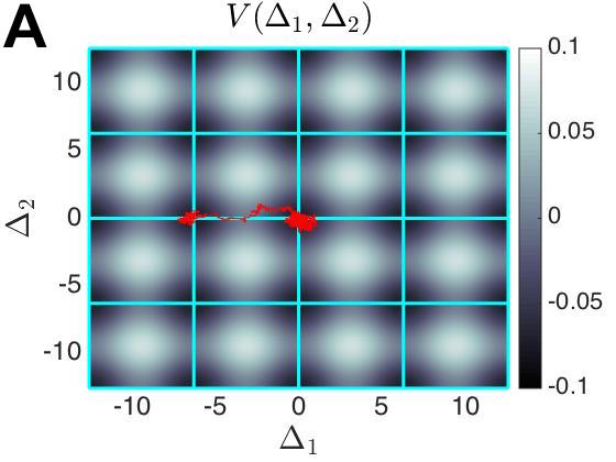
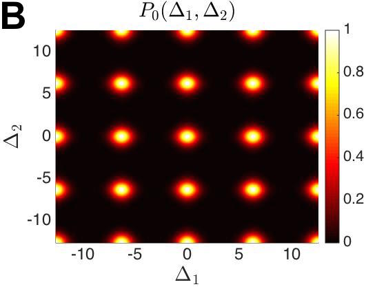
Refer to caption
Refer to caption
Fig. 7: Nonlinear dynamics in the input driven neural field (44) on the plane 2superscript2{\mathbb{R}}^{2} with Heaviside firing rate (4) and Bessel function weight (2), subject to the periodic input I~(𝐱)=0.3(cosx1+cosx2)~𝐼𝐱0.3subscript𝑥1subscript𝑥2\tilde{I}({\mathbf{x}})=0.3(\cos x_{1}+\cos x_{2}). (A) Bump position (thin line) sampled from a single realization of the system (44) for t[0,4000]𝑡04000t\in[0,4000], superimposed on a plot of the potential V(𝚫)𝑉𝚫V({\bm{\Delta}}). Over long periods of time, the stochastically-driven position of bumps tends to dwell primarily in the vicinity of minima of the potential V(𝚫)𝑉𝚫V({\bm{\Delta}}) defined by (68). However, there are rare events whereby the bump transitions to a neighboring potential well. Thick lines represent the paths of least action between attractors at (2mπ,2nπ)2𝑚𝜋2𝑛𝜋(2m\pi,2n\pi), m,n𝑚𝑛m,n\in{\mathbb{Z}}. (B) Re-normalized stationary probability density P0(𝐱)subscript𝑃0𝐱P_{0}({\mathbf{x}}) (so that P0(𝐱)max=1subscriptnormsubscript𝑃0𝐱𝑚𝑎𝑥1||P_{0}({\mathbf{x}})||_{max}=1, otherwise P0(𝐱)subscript𝑃0𝐱P_{0}({\mathbf{x}}) would be infinitesimally small everywhere) has peaks at the minima of the potential function V(𝚫)𝑉𝚫V({\bm{\Delta}}). Parameters are ε=0.025𝜀0.025\varepsilon=0.025, κ=0𝜅0\kappa=0, and weight w𝑤w is (19) with [c1,c2,c3,c4]=[5/3,5/3,1/2,1/2]subscript𝑐1subscript𝑐2subscript𝑐3subscript𝑐453531212[c_{1},c_{2},c_{3},c_{4}]=[5/3,-5/3,-1/2,1/2].

The stochastic dynamics is shaped by an underlying potential function V(𝚫)𝑉𝚫V({\bm{\Delta}}), which is the solution to the pair of equations

dVdΔ1=ε1/2G1(𝚫),dVdΔ2=ε1/2G2(𝚫),formulae-sequence𝑑𝑉𝑑subscriptΔ1superscript𝜀12subscript𝐺1𝚫𝑑𝑉𝑑subscriptΔ2superscript𝜀12subscript𝐺2𝚫\displaystyle\frac{dV}{d\Delta_{1}}=\varepsilon^{1/2}G_{1}({\bm{\Delta}}),\hskip 14.22636pt\frac{dV}{d\Delta_{2}}=\varepsilon^{1/2}G_{2}({\bm{\Delta}}), (61)

so that the attractors of the noise free system are the minima of V(𝚫)𝑉𝚫V({\bm{\Delta}}). While (61) cannot always be solved explicitly, we will present an example below where they can, for illustration. To analyze the system, we reformulate (52) as an equivalent Fokker-Planck equation [27]

P(𝚫,t)t=j=12{Δj[ε1/2Gj(𝚫)P(𝚫,t)]+εDj2P(𝚫,t)Δj2},𝑃𝚫𝑡𝑡superscriptsubscript𝑗12subscriptΔ𝑗delimited-[]superscript𝜀12subscript𝐺𝑗𝚫𝑃𝚫𝑡𝜀subscript𝐷𝑗superscript2𝑃𝚫𝑡superscriptsubscriptΔ𝑗2\displaystyle\frac{\partial P({\bm{\Delta}},t)}{\partial t}=\sum_{j=1}^{2}\left\{\frac{\partial}{\partial\Delta_{j}}\left[\varepsilon^{1/2}G_{j}({\bm{\Delta}})P({\bm{\Delta}},t)\right]+\varepsilon D_{j}\frac{\partial^{2}P({\bm{\Delta}},t)}{\partial\Delta_{j}^{2}}\right\}, (62)

where P(𝚫,t)𝑃𝚫𝑡P({\bm{\Delta}},t) is the probability of finding the bump at position 𝚫=(Δ1,Δ2)𝚫subscriptΔ1subscriptΔ2{\bm{\Delta}}=(\Delta_{1},\Delta_{2}) at time t𝑡t. Assuming there is a single stable attractor defined by the potential V(𝚫)𝑉𝚫V({\bm{\Delta}}), in the long time limit

limtP(𝚫,t)=P0(𝚫)=χexp[V(𝚫)εD],subscript𝑡𝑃𝚫𝑡subscript𝑃0𝚫𝜒𝑉𝚫𝜀𝐷\displaystyle\lim_{t\to\infty}P({\bm{\Delta}},t)=P_{0}({\bm{\Delta}})=\chi\exp\left[-\frac{V({\bm{\Delta}})}{\varepsilon D}\right], (63)

in the case of rotationally symmetric noise D1=D2=Dsubscript𝐷1subscript𝐷2𝐷D_{1}=D_{2}=D, where χ𝜒\chi is a normalization factor such that 2P0(𝚫)𝑑𝚫=1subscriptsuperscript2subscript𝑃0𝚫differential-d𝚫1\int_{{\mathbb{R}}^{2}}P_{0}({\bm{\Delta}})d{\bm{\Delta}}=1. The long time variance 𝚫2=Δ12+Δ22delimited-⟨⟩superscriptnorm𝚫2delimited-⟨⟩superscriptsubscriptΔ12delimited-⟨⟩superscriptsubscriptΔ22\langle||{\bm{\Delta}}||^{2}\rangle=\langle\Delta_{1}^{2}\rangle+\langle\Delta_{2}^{2}\rangle is thus given by the integral

Δ12+Δ22=2(Δ12+Δ22)P0(𝚫)𝑑𝚫.delimited-⟨⟩superscriptsubscriptΔ12delimited-⟨⟩superscriptsubscriptΔ22subscriptsuperscript2superscriptsubscriptΔ12superscriptsubscriptΔ22subscript𝑃0𝚫differential-d𝚫\displaystyle\langle\Delta_{1}^{2}\rangle+\langle\Delta_{2}^{2}\rangle=\int_{{\mathbb{R}}^{2}}(\Delta_{1}^{2}+\Delta_{2}^{2})P_{0}({\bm{\Delta}})d{\bm{\Delta}}. (64)

To demonstrate our analysis on a specific example, we focus on an input which allows explicit computation of the steady state distribution. Thus, we take the external input I~(𝐱)=A0(cosx1+cosx2)~𝐼𝐱subscript𝐴0subscript𝑥1subscript𝑥2\tilde{I}({\mathbf{x}})=A_{0}(\cos x_{1}+\cos x_{2}) and assume we then wish to compute the statistics of the stationary probability density P0(𝚫)subscript𝑃0𝚫P_{0}({\bm{\Delta}}). Furthermore, we take the Heaviside firing rate function (4), then the integrals (53) can be simplified by making the substitutions x1=rcosθsubscript𝑥1𝑟𝜃x_{1}=r\cos\theta and x2=rsinθsubscript𝑥2𝑟𝜃x_{2}=r\sin\theta and integrating out the radial coordinate r𝑟r, so

G1(𝚫)subscript𝐺1𝚫\displaystyle G_{1}({\bm{\Delta}}) =U(a)02πcos(θ)I~(𝐚+𝚫)𝑑θU(a)202πcos2θdθ=1U(a)π02πcos(θ)I~(𝐚+𝚫)𝑑θabsentsuperscript𝑈𝑎superscriptsubscript02𝜋𝜃~𝐼𝐚𝚫differential-d𝜃superscript𝑈superscript𝑎2superscriptsubscript02𝜋superscript2𝜃𝑑𝜃1superscript𝑈𝑎𝜋superscriptsubscript02𝜋𝜃~𝐼𝐚𝚫differential-d𝜃\displaystyle=\frac{U^{\prime}(a)\int_{0}^{2\pi}\cos(\theta)\tilde{I}({\mathbf{a}}+{\bm{\Delta}})d\theta}{U^{\prime}(a)^{2}\int_{0}^{2\pi}\cos^{2}\theta d\theta}=\frac{1}{U^{\prime}(a)\pi}\int_{0}^{2\pi}\cos(\theta)\tilde{I}({\mathbf{a}}+{\bm{\Delta}})d\theta (65)
G2(𝚫)subscript𝐺2𝚫\displaystyle G_{2}({\bm{\Delta}}) =U(a)02πsin(θ)I~(𝐚+𝚫)𝑑θU(a)202πsin2θdθ=1U(a)π02πsinθI~(𝐚+𝚫)𝑑θ,absentsuperscript𝑈𝑎superscriptsubscript02𝜋𝜃~𝐼𝐚𝚫differential-d𝜃superscript𝑈superscript𝑎2superscriptsubscript02𝜋superscript2𝜃𝑑𝜃1superscript𝑈𝑎𝜋superscriptsubscript02𝜋𝜃~𝐼𝐚𝚫differential-d𝜃\displaystyle=\frac{U^{\prime}(a)\int_{0}^{2\pi}\sin(\theta)\tilde{I}({\mathbf{a}}+{\bm{\Delta}})d\theta}{U^{\prime}(a)^{2}\int_{0}^{2\pi}\sin^{2}\theta d\theta}=\frac{1}{U^{\prime}(a)\pi}\int_{0}^{2\pi}\sin\theta\tilde{I}({\mathbf{a}}+{\bm{\Delta}})d\theta, (66)

where 𝐚=(a,θ)𝐚𝑎𝜃{\mathbf{a}}=(a,\theta). Selecting the doubly periodic function for our external input I~(𝐱)=A0(cosx1+cosx2)~𝐼𝐱subscript𝐴0subscript𝑥1subscript𝑥2\tilde{I}({\mathbf{x}})=A_{0}(\cos x_{1}+\cos x_{2}), we generate terms similar to those that arose in our explicit calculation of the diffusion coefficient Djsubscript𝐷𝑗D_{j} (43). Subsequently, we find we can evaluate these explicitly, to arrive at the compact expression

Gj(𝚫)=2A0J1(a)U(a)sin(Δj),{j=1,2}.subscript𝐺𝑗𝚫2subscript𝐴0subscript𝐽1𝑎superscript𝑈𝑎subscriptΔ𝑗𝑗12\displaystyle G_{j}({\bm{\Delta}})=-\frac{2A_{0}J_{1}(a)}{U^{\prime}(a)}\sin(\Delta_{j}),\ \ \ \ \ \{j=1,2\}. (67)

Thus, the positions Δ1subscriptΔ1\Delta_{1} and Δ2subscriptΔ2\Delta_{2} evolve independently in nonlinear system (52), in the case of this specific input function. Thus, it is straightforward to evaluate the potential function as the solution to (61), finding

V(𝚫)=2ε1/2A0J1(a)|U(a)|[cos(Δ1)+cos(Δ2)],𝑉𝚫2superscript𝜀12subscript𝐴0subscript𝐽1𝑎superscript𝑈𝑎delimited-[]subscriptΔ1subscriptΔ2\displaystyle V({\bm{\Delta}})=-\frac{2\varepsilon^{1/2}A_{0}J_{1}(a)}{|U^{\prime}(a)|}\left[\cos(\Delta_{1})+\cos(\Delta_{2})\right], (68)

which can then be utilized to compute the statistics of the stationary probability density (63). We demonstrate that stochastic trajectories of the bump tend to dwell mostly in the minima of the potential function defined by (68) in Fig. 7A. Such durations are interrupted by abrupt transitions of the bump between neighboring wells as in the one-dimensional case [36]. An example of the rescaled stationary probability density is given in Fig. 7B. We save a more thorough analysis of these results for subsequent work.

5 Discussion

We have analyzed the impact of additive noise on the stochastic motion of bumps in planar neural field equations. In networks with no spatial heterogeneity, noise causes bumps to wander according to two-dimensional Brownian motion. The diffusion coefficient associated with this motion can be approximated using an asymptotic expansion that treats the impact of noise perturbatively. Assuming the bump retains its profile, to first order, we can derive an effective diffusion equation for the bump’s position as a function of time. Notably, the dynamics of the bumps can be separated into diffusion along the canonical directions (x1,x2subscript𝑥1subscript𝑥2x_{1},x_{2}) in 2superscript2{\mathbb{R}}^{2}. In the presence of spatially heterogeneous external inputs, the stochastic bumps no longer obey dynamics well described by pure diffusion. Rather, bumps are attracted to the local maxima of the input functions, so their motion can be approximated by multivariate Ornstein-Uhlenbeck processes. In particular, we find that the geometry of the external inputs define the manifold to which bumps are attracted. Radially symmetric inputs attract bumps to a single point and translationally symmetric peaked inputs attract bumps to a one-dimensional line through 2superscript2{\mathbb{R}}^{2}.

Our primary motivation for exploring these models comes from extensive experimental literature on persistent activity representing spatial working memory [26, 42]. Particularly pertinent to this work are place cell and grid cell networks, which track a mammal’s idiothetic position in two-dimensional space as it navigates through its environment [43]. Networks in cortex and hippocampus are capable of encoding analog spatial variables for time periods lasting seconds up to tens of minutes on length scales of hundreds of meters [29]. The specific single neuron and network architectural features that engender this impressive accuracy are the subject of ongoing research [15]. We will extend the results presented here in future work by addressing how spatially heterogeneous architecture[36, 37] and the known multilayered structure of grid cell networks [29, 14] may contribute to the observed precision of spatial navigation networks of the brain. Thus, we will extend the methods we have developed for analyzing coupling between multiple layers of one-dimensional stochastic neural fields to two-dimensions [33, 12]. Furthermore, it is important to note that synaptic connections projecting from long-range axons can be subject to axonal transmission delays, as in the planar neural field study of Hutt and Rougier [31]. In future work, we plan to explore the impact of delays within and between layers of planar neural fields on the stochastic motion of bumps, as we did in our recent work on one-dimensional systems [34].

Lastly, we aim to extend this work by further analyzing the impact of external inputs on the stochastic dynamics of bumps in planar neural fields. As we found here, the local maxima of external inputs determine the most likely spatial regions to find bumps that are perturbed by spatiotemporal noise. However, this general picture may change if we consider external inputs that vary in time. For instance, stationary external inputs that turn on and off periodically will likely not pin bumps in place as well. In a similar way, we could explore how well bumps track the positions inputs that move smoothly in space, dependent on their speed. It is possible that noise may actually improve bumps’ tracking of external input positions, in some parameter regimes. We may be able to exploit relative slow or fast timescales of external inputs to extend our presented asymptotic analysis, which assumes inputs are stationary.

References

  • [1] A. Abbott, Neuroscience: Brains of norway., Nature, 514 (2014), pp. 154–157.
  • [2] S. Amari, Dynamics of pattern formation in lateral-inhibition type neural fields, Biol. Cybern., 27 (1977), pp. 77–87.
  • [3]  , Heaviside world: Excitation and self-organization of neural fields, in Neural Fields: Theory and Applications, S. Coombes, P. beim Graben, R. Potthast, and J. Wright, eds., Springer, 2014.
  • [4] S. I. Amari, Mathematical theory of nerve nets, Sangyotosho, 1978.
  • [5] J. Armero, J. Casademunt, L. Ramirez-Piscina, and J. Sancho, Ballistic and diffusive corrections to front propagation in the presence of multiplicative noise, Physical Review E, 58 (1998), p. 5494.
  • [6] M. Benayoun, J. D. Cowan, W. van Drongelen, and E. Wallace, Avalanches in a stochastic model of spiking neurons, PLoS computational biology, 6 (2010), p. e1000846.
  • [7] C. A. Brackley and M. S. Turner, Random fluctuations of the firing rate function in a continuum neural field model, Phys. Rev. E, 75 (2007), p. 041913.
  • [8] P. C. Bressloff, Spatiotemporal dynamics of continuum neural fields, Journal of Physics A: Mathematical and Theoretical, 45 (2012), p. 033001.
  • [9] P. C. Bressloff and S. Coombes, Neural ’bubble’ dynamics revisited, Cognit Comput, 5 (2013), pp. 281–294.
  • [10] P. C. Bressloff and J. D. Cowan, A spherical model for orientation and spatial–frequency tuning in a cortical hypercolumn, Philosophical Transactions of the Royal Society of London. Series B: Biological Sciences, 358 (2003), pp. 1643–1667.
  • [11] P. C. Bressloff and Z. P. Kilpatrick, Two-dimensional bumps in piecewise smooth neural fields with synaptic depression, SIAM Journal on Applied Mathematics, 71 (2011), pp. 379–408.
  • [12] P. C. Bressloff and Z. P. Kilpatrick, Nonlinear langevin equations for wandering patterns in stochastic neural fields, SIAM Journal on Applied Dynamical Systems, 14 (2015), pp. 305–334.
  • [13] P. C. Bressloff and M. A. Webber, Front propagation in stochastic neural fields, SIAM Journal on Applied Dynamical Systems, 11 (2012), pp. 708–740.
  • [14] V. H. Brun, T. Solstad, K. B. Kjelstrup, M. Fyhn, M. P. Witter, E. I. Moser, and M.-B. Moser, Progressive increase in grid scale from dorsal to ventral medial entorhinal cortex, Hippocampus, 18 (2008), pp. 1200–1212.
  • [15] Y. Burak and I. R. Fiete, Accurate path integration in continuous attractor network models of grid cells, PLoS Comput Biol, 5 (2009), p. e1000291.
  • [16] N. Burgess, E. A. Maguire, and J. O’Keefe, The human hippocampus and spatial and episodic memory, Neuron, 35 (2002), pp. 625–641.
  • [17] S. Coombes and M. Owen, Exotic dynamics in a firing rate model of neural tissue with threshold accommodation, in Fluids and Waves: Recent Trends in Applied Analysis, F. Botelho, T. Hagen, and J. E. Jamison, eds., vol. 440, American Mathematical Society: Contemporary Mathematics, 2007, pp. 123–144.
  • [18] S. Coombes, H. Schmidt, and I. Bojak, Interface dynamics in planar neural field models, J Math Neurosci, 2 (2012), p. 9.
  • [19] A. Destexhe and D. Contreras, Neuronal computations with stochastic network states, Science, 314 (2006), pp. 85–90.
  • [20] A. A. Faisal, L. P. Selen, and D. M. Wolpert, Noise in the nervous system, Nature Reviews Neuroscience, 9 (2008), pp. 292–303.
  • [21] O. Faugeras and J. Inglis, Stochastic neural field equations: A rigorous footing, Journal of mathematical biology, (2013), pp. 1–42.
  • [22] O. Faugeras, R. Veltz, and F. Grimbert, Persistent neural states: stationary localized activity patterns in nonlinear continuous n-population, q-dimensional neural networks, Neural computation, 21 (2009), pp. 147–187.
  • [23] S. E. Folias and P. C. Bressloff, Breathing pulses in an excitatory neural network, SIAM Journal on Applied Dynamical Systems, 3 (2004), pp. 378–407.
  • [24] S. E. Folias and P. C. Bressloff, Breathers in two-dimensional neural media, Phys Rev Lett, 95 (2005), p. 208107.
  • [25] M. D. Fox and M. E. Raichle, Spontaneous fluctuations in brain activity observed with functional magnetic resonance imaging, Nature Reviews Neuroscience, 8 (2007), pp. 700–711.
  • [26] S. Funahashi, C. J. Bruce, P. S. Goldman-Rakic, et al., Mnemonic coding of visual space in the monkey’s dorsolateral prefrontal cortex, J Neurophysiol, 61 (1989), pp. 331–349.
  • [27] C. W. Gardiner, Handbook of stochastic methods for physics, chemistry, and the natural sciences, Springer-Verlag, Berlin, 3rd ed ed., 2004.
  • [28] P. Goldman-Rakic, Cellular basis of working memory, Neuron, 14 (1995), pp. 477–485.
  • [29] T. Hafting, M. Fyhn, S. Molden, M.-B. Moser, and E. I. Moser, Microstructure of a spatial map in the entorhinal cortex, Nature, 436 (2005), pp. 801–806.
  • [30] A. Hutt, A. Longtin, and L. Schimansky-Geier, Additive noise-induced turing transitions in spatial systems with application to neural fields and the swift–hohenberg equation, Physica D, 237 (2008), pp. 755–773.
  • [31] A. Hutt and N. P. Rougier, Activity spread and breathers induced by finite transmission speeds in two-dimensional neural fields, Physical Review E: Statistical, Nonlinear, and Soft Matter Physics, 82 (2010), p. R055701.
  • [32] S. Katzner, I. Nauhaus, A. Benucci, V. Bonin, D. L. Ringach, and M. Carandini, Local origin of field potentials in visual cortex, Neuron, 61 (2009), pp. 35–41.
  • [33] Z. P. Kilpatrick, Interareal coupling reduces encoding variability in multi-area models of spatial working memory, Frontiers in Computational Neuroscience, 7 (2013).
  • [34]  , Delay stabilizes stochastic motion of bumps in layered neural fields, Physica D: Nonlinear Phenomena, 295 (2015), pp. 30–45.
  • [35] Z. P. Kilpatrick and P. C. Bressloff, Spatially structured oscillations in a two-dimensional excitatory neuronal network with synaptic depression, Journal of computational neuroscience, 28 (2010), pp. 193–209.
  • [36] Z. P. Kilpatrick and B. Ermentrout, Wandering bumps in stochastic neural fields, SIAM J. Appl. Dyn. Syst., 12 (2013), pp. 61–94.
  • [37] Z. P. Kilpatrick, B. Ermentrout, and B. Doiron, Optimizing working memory with heterogeneity of recurrent cortical excitation, J Neurosci, 33 (2013), pp. 18999–9011.
  • [38] J. Kruger and W. Stannat, Front propagation in stochastic neural fields: A rigorous mathematical framework, SIAM Journal on Applied Dynamical Systems, 13 (2014), pp. 1293–1310.
  • [39] C. R. Laing and A. Longtin, Noise-induced stabilization of bumps in systems with long-range spatial coupling, Physica D: Nonlinear Phenomena, 160 (2001), pp. 149–172.
  • [40] C. R. Laing and W. C. Troy, Pde methods for nonlocal models, SIAM Journal on Applied Dynamical Systems, 2 (2003), pp. 487–516.
  • [41] C. R. Laing, W. C. Troy, B. Gutkin, and G. B. Ermentrout, Multiple bumps in a neuronal model of working memory, SIAM Journal on Applied Mathematics, 63 (2002), pp. 62–97.
  • [42] B. L. McNaughton, F. P. Battaglia, O. Jensen, E. I. Moser, and M.-B. Moser, Path integration and the neural basis of the’cognitive map’, Nature Reviews Neuroscience, 7 (2006), pp. 663–678.
  • [43] E. I. Moser, E. Kropff, and M.-B. Moser, Place cells, grid cells, and the brain’s spatial representation system, Annual Review of Neuroscience, 31 (2008), p. 69.
  • [44] M. Owen, C. Laing, and S. Coombes, Bumps and rings in a two-dimensional neural field: splitting and rotational instabilities, New Journal of Physics, 9 (2007), p. 378.
  • [45] D. Panja, Effects of fluctuations on propagating fronts, Physics Reports, 393 (2004), pp. 87–174.
  • [46] F. Sagués, J. M. Sancho, and J. García-Ojalvo, Spatiotemporal order out of noise, Reviews of Modern Physics, 79 (2007), p. 829.
  • [47] J. Taylor, Neural ‘bubble’ dynamics in two dimensions: foundations, Biological Cybernetics, 80 (1999), pp. 393–409.
  • [48] C. van Vreeswijk and H. Sompolinsky, Chaos in neuronal networks with balanced excitatory and inhibitory activity, Science, 274 (1996), pp. 1724–1726.
  • [49] X.-J. Wang, Synaptic reverberation underlying mnemonic persistent activity, Trends in neurosciences, 24 (2001), pp. 455–463.
  • [50]  , Neurophysiological and computational principles of cortical rhythms in cognition, Physiol Rev, 90 (2010), pp. 1195–268.
  • [51] B. Weber, C. Burger, M. Wyss, G. Von Schulthess, F. Scheffold, and A. Buck, Optical imaging of the spatiotemporal dynamics of cerebral blood flow and oxidative metabolism in the rat barrel cortex, European Journal of Neuroscience, 20 (2004), pp. 2664–2670.
  • [52] H. Werner and T. Richter, Circular stationary solutions in two-dimensional neural fields., Biol. Cybern., 85 (2001), pp. 211–217.
  • [53] H. R. Wilson and J. D. Cowan, Excitatory and inhibitory interactions in localized populations of model neurons, Biophysical journal, 12 (1972), pp. 1–24.
  • [54] K. Wimmer, D. Q. Nykamp, C. Constantinidis, and A. Compte, Bump attractor dynamics in prefrontal cortex explains behavioral precision in spatial working memory, Nature neuroscience, 17 (2014), pp. 431–439.
  • [55] M. M. Yartsev and N. Ulanovsky, Representation of three-dimensional space in the hippocampus of flying bats, Science, 340 (2013), pp. 367–372.