Low-complexity modeling of partially available second-order statistics: theory and an efficient matrix completion algorithm

Armin Zare, Yongxin Chen, Mihailo R. Jovanović, and Tryphon T. Georgiou Financial support from the National Science Foundation under Award CMMI 1363266, the Air Force Office of Scientific Research under Award FA9550-16-1-0009, the University of Minnesota Informatics Institute Transdisciplinary Faculty Fellowship, and the University of Minnesota Doctoral Dissertation Fellowship is gratefully acknowledged. Armin Zare, Yongxin Chen, Mihailo R. Jovanović and Tryphon T. Georgiou are with the Department of Electrical and Computer Engineering, University of Minnesota, Minneapolis, MN 55455. E-mails: arminzare@umn.edu, chen2468@umn.edu, mihailo@umn.edu, tryphon@umn.edu.
Abstract

State statistics of linear systems satisfy certain structural constraints that arise from the underlying dynamics and the directionality of input disturbances. In the present paper we study the problem of completing partially known state statistics. Our aim is to develop tools that can be used in the context of control-oriented modeling of large-scale dynamical systems. For the type of applications we have in mind, the dynamical interaction between state variables is known while the directionality and dynamics of input excitation is often uncertain. Thus, the goal of the mathematical problem that we formulate is to identify the dynamics and directionality of input excitation in order to explain and complete observed sample statistics. More specifically, we seek to explain correlation data with the least number of possible input disturbance channels. We formulate this inverse problem as rank minimization, and for its solution, we employ a convex relaxation based on the nuclear norm. The resulting optimization problem is cast as a semidefinite program and can be solved using general-purpose solvers. For problem sizes that these solvers cannot handle, we develop a customized alternating minimization algorithm (AMA). We interpret AMA as a proximal gradient for the dual problem and prove sub-linear convergence for the algorithm with fixed step-size. We conclude with an example that illustrates the utility of our modeling and optimization framework and draw contrast between AMA and the commonly used alternating direction method of multipliers (ADMM) algorithm.

Index Terms:
Alternating minimization algorithm, convex optimization, disturbance dynamics, low-rank approximation, matrix completion problems, nuclear norm regularization, structured covariances.

I Introduction

Motivation for this work stems from control-oriented modeling of systems with a large number of degrees of freedom. Indeed, dynamics governing many physical systems are prohibitively complex for purposes of control design and optimization. Thus, it is common practice to investigate low-dimensional models that preserve the essential dynamics. To this end, stochastically driven linearized models often represent an effective option that is also capable of explaining observed statistics. Further, such models are well-suited for analysis and synthesis using tools from modern robust control.

An example that illustrates the point is the modeling of fluid flows. In this, the Navier-Stokes equations are prohibitively complex for control design [1]. On the other hand, linearization of the equations around the mean-velocity profile in the presence of stochastic excitation has been shown to qualitatively replicate structural features of shear flows [2, 3, 4, 5, 6, 7, 8, 9, 10]. However, it has also been recognized that a simple white-in-time stochastic excitation cannot reproduce important statistics of the fluctuating velocity field [11, 12]. In this paper, we introduce a mathematical framework to consider stochastically driven linear models that depart from the white-in-time restriction on random disturbances. Our objective is to identify low-complexity disturbance models that account for partially available second-order statistics of large-scale dynamical systems.

Thus, herein, we formulate a covariance completion problem for linear time-invariant (LTI) systems with uncertain disturbance dynamics. The complexity of the disturbance model is quantified by the number of input channels. We relate the number of input channels to the rank of a certain matrix which reflects the directionality of input disturbances and the correlation structure of excitation sources. We address the resulting optimization problem using the nuclear norm as a surrogate for rank [13, 14, 15, 16, 17, 18, 19, 20].

The relaxed optimization problem is convex and can be cast as a semidefinite program (SDP) which is readily solvable by standard software for small-size problems. A further contribution is to specifically address larger problems that general-purpose solvers cannot handle. To this end, we exploit the problem structure, derive the Lagrange dual, and develop an efficient customized Alternating Minimization Algorithm (AMA). Specifically, we show that AMA is a proximal gradient for the dual and establish convergence for the covariance completion problem. We utilize a Barzilai-Borwein (BB) step-size initialization followed by backtracking to achieve sufficient dual ascent. This enhances convergence relative to theoretically-proven sub-linear convergence rates for AMA with fixed step-size. We also draw contrast between AMA and the commonly used Alternating Direction Method of Multipliers (ADMM) by showing that AMA leads to explicit, easily computable updates of both primal and dual optimization variables.

The solution to the covariance completion problem gives rise to a class of linear filters that realize colored-in-time disturbances and account for the observed state statistics. This is a non-standard stochastic realization problem with partial spectral information [21, 22, 23, 24]. The class of modeling filters that we generate for the stochastic excitation is generically minimal in the sense that it has the same number of degrees of freedom as the original linear system. Furthermore, we demonstrate that the covariance completion problem can be also interpreted as an identification problem that aims to explain available statistics via suitable low-rank dynamical perturbations.

Our presentation is organized as follows. We summarize key results regarding the structure of state covariances and its relation to the power spectrum of input processes in Section II. We characterize admissible signatures for matrices that parametrize disturbance spectra and formulate the covariance completion problem in Section III. Section IV develops an efficient optimization algorithm for solving this problem in large dimensions. To highlight the theoretical and algorithmic developments we provide an example in Section V. We conclude with remarks and future directions in Section VI.

II Linear stochastic models and state statistics

We now discuss algebraic conditions that state covariances of LTI systems satisfy. For white-in-time stochastic inputs state statistics satisfy an algebraic Lyapunov equation. A similar algebraic characterization holds for LTI systems driven by colored stochastic processes [25, 26]. This characterization provides the foundation for the covariance completion problem that we study in this paper.

Consider a linear time-invariant system

x˙=Ax+Buy=Cx˙𝑥𝐴𝑥𝐵𝑢𝑦𝐶𝑥\begin{array}[]{rcl}\dot{x}&\!\!=\!\!&A\,x\;+\;B\,u\\[2.84544pt] {y}&\!\!{=}\!\!&{C\,x}\end{array} (1)

where x(t)n𝑥𝑡superscript𝑛x(t)\in\mathbb{C}^{n} is a state vector, y(t)p𝑦𝑡superscript𝑝y(t)\in\mathbb{C}^{p} is the output, and u(t)m𝑢𝑡superscript𝑚u(t)\in\mathbb{C}^{m} is a zero-mean stationary stochastic input. The dynamic matrix An×n𝐴superscript𝑛𝑛A\in\mathbb{C}^{n\times n} is Hurwitz, Bn×m𝐵superscript𝑛𝑚B\in\mathbb{C}^{n\times m} is the input matrix with mn𝑚𝑛m\leq n, and (A,B)𝐴𝐵(A,B) is a controllable pair. Let X𝑋X be the steady-state covariance of the state vector of system (1), X=limt𝐄(x(t)x(t))𝑋subscript𝑡𝐄𝑥𝑡superscript𝑥𝑡X=\lim_{t\to\infty}{\mathbf{E}}\left(x(t)x^{*}(t)\right), with 𝐄𝐄{\mathbf{E}} being the expectation operator. We next review key results and provide new insights into the following questions:

  • (i)

    What is the algebraic structure of X𝑋X? In other words, given a positive definite matrix X𝑋X, under what conditions does it qualify to be the steady-state covariance of (1)?

  • (ii)

    Given the steady-state covariance X𝑋X of (1), what can be said about the power spectra of input processes that are consistent with these statistics?

II-A Algebraic constraints on admissible covariances

The steady-state covariance matrix X𝑋X of the state vector in (1) satisfies [25, 26]

rank[AX+XABB0]=rank[0BB0].rankmatrix𝐴𝑋𝑋superscript𝐴𝐵superscript𝐵0rankmatrix0𝐵superscript𝐵0\operatorname*{rank}\left[\begin{matrix}AX\,+\,XA^{*}&B\\ B^{*}&0\end{matrix}\right]\,=\;\operatorname*{rank}\left[\begin{matrix}0&B\\ B^{*}&0\end{matrix}\right]. (2a)
An equivalent characterization is that there is a solution Hn×m𝐻superscript𝑛𝑚H\in\mathbb{C}^{n\times m} to the equation
AX+XA=BHHB.𝐴𝑋𝑋superscript𝐴𝐵superscript𝐻𝐻superscript𝐵A\,X\;+\;XA^{*}\;=\;-BH^{*}\;-\;HB^{*}. (2b)

Either of these conditions, together with the positive definiteness of X𝑋X, completely characterize state covariances of linear dynamical systems driven by white or colored stochastic processes [25, 26]. When the input u𝑢u is white noise with covariance W𝑊W, X𝑋X satisfies the algebraic Lyapunov equation

AX+XA=BWB.𝐴𝑋𝑋superscript𝐴𝐵𝑊superscript𝐵A\,X\;+\;XA^{*}\;=\;-B\,WB^{*}.

In this case, H𝐻H in (2b) is determined by H=12BW𝐻12𝐵𝑊H=\frac{1}{2}BW and the right-hand-side BWB𝐵𝑊superscript𝐵-B\,WB^{*} is sign-definite. In fact, except for this case when the input is white noise, the matrix Z𝑍Z defined by

Z𝑍\displaystyle Z :=:absent\displaystyle\!\!\mathrel{\mathop{:}}=\!\! (AX+XA)𝐴𝑋𝑋superscript𝐴\displaystyle-\left(AX\,+\,XA^{*}\right) (3a)
=\displaystyle\!\!=\!\! BH+HB𝐵superscript𝐻𝐻superscript𝐵\displaystyle BH^{*}\,+\,HB^{*} (3b)

may have both positive and negative eigenvalues. Additional discussion on the structure of Z𝑍Z is provided in Section III-A.

II-B Power spectrum of input process

filterlinearsystemlinearsystem\begin{array}[]{c}\mbox{linear}\\ \mbox{system}\end{array}whitenoisewhitenoise\begin{array}[]{c}\mbox{white}\\ \mbox{noise}\end{array}w𝑤wx𝑥xcolorednoisecolorednoise\begin{array}[]{c}\mbox{colored}\\ \mbox{noise}\end{array}u𝑢u
(a)
linearsystemlinearsystem\begin{array}[]{c}\mbox{linear}\\ \mbox{system}\end{array}K𝐾-K++whitenoisewhitenoise\begin{array}[]{c}\mbox{white}\\ \mbox{noise}\end{array}w𝑤wx𝑥xcolorednoisecolorednoise\begin{array}[]{c}\mbox{colored}\\ \mbox{noise}\end{array}u𝑢u
(b)
Figure 1: (a) A cascade connection of an LTI system with a linear filter that is designed to account for the sampled steady-state covariance matrix X𝑋X; (b) An equivalent feedback representation of the cascade connection in (a).

For stochastically-driven LTI systems the state statistics can be obtained from knowledge of the system model and the input statistics. Herein, we are interested in the converse: starting from the steady-state covariance X𝑋X and the system dynamics (1), we want to identify the power spectrum of the input process u𝑢u. As illustrated in Fig. 1a, we seek to construct a filter which, when driven by white noise, produces a suitable stationary input u𝑢u to (1) so that the state covariance is X𝑋X. Next, we characterize a class of filters with degree at most n𝑛n.

Consider the linear filter given by

ξ˙˙𝜉\displaystyle\dot{\xi} =\displaystyle\!\!=\!\! (ABK)ξ+Bw𝐴𝐵𝐾𝜉𝐵𝑤\displaystyle(A\,-\,BK)\,\xi\;+\;B\,w (4a)
u𝑢\displaystyle u =\displaystyle\!\!=\!\! Kξ+w𝐾𝜉𝑤\displaystyle-K\,\xi\;+\;w (4b)
where w𝑤w is a zero-mean white stochastic process with covariance Ω0succeedsΩ0\Omega\succ 0 and
K=12ΩBX1HX1,𝐾12Ωsuperscript𝐵superscript𝑋1superscript𝐻superscript𝑋1K\;=\;\frac{1}{2}\,\Omega\,B^{*}X^{-1}\;-\;H^{*}X^{-1}, (4c)

for some H𝐻H that satisfies (2b). The power spectrum of u𝑢u is determined by

Πuu(ω)=Ψ(jω)ΩΨ(jω)subscriptΠ𝑢𝑢𝜔Ψ𝑗𝜔ΩsuperscriptΨ𝑗𝜔\Pi_{uu}(\omega)\;=\;\Psi(j\omega)\,\Omega\,\Psi^{*}(j\omega)

where

Ψ(s)=IK(sIA+BK)1BΨ𝑠𝐼𝐾superscript𝑠𝐼𝐴𝐵𝐾1𝐵\Psi(s)\;=\;I\;-\;K\,(sI\,-\,A\,+\,BK)^{-1}B

is the transfer function of the filter (4). To verify this, consider the cascade connection shown in Fig. 1a, with state space representation

[x˙ξ˙]=[ABK0ABK][xξ]+[BB]wx=[I0][xξ].delimited-[]˙𝑥˙𝜉delimited-[]𝐴𝐵𝐾0𝐴𝐵𝐾delimited-[]𝑥𝜉delimited-[]𝐵𝐵𝑤𝑥delimited-[]𝐼0delimited-[]𝑥𝜉\begin{array}[]{rcl}\left[\begin{array}[]{c}\dot{x}\\ \dot{\xi}\end{array}\right]&\!\!=\!\!&\left[\begin{array}[]{cc}A&-BK\\ 0&A\,-\,BK\end{array}\right]\left[\begin{array}[]{c}x\\ \xi\end{array}\right]\,+\,\left[\begin{array}[]{c}B\\ B\end{array}\right]w\\ x&\!\!=\!\!&\left[\begin{array}[]{cc}I&0\end{array}\right]\left[\begin{array}[]{c}x\\ \xi\end{array}\right].\end{array} (5)

This representation has twice as many states as linear system (1), but it is not controllable and therefore not minimal. The coordinate transformation

[xϕ]=[I0II][xξ]delimited-[]𝑥italic-ϕdelimited-[]𝐼0𝐼𝐼delimited-[]𝑥𝜉\left[\begin{array}[]{c}x\\ \phi\end{array}\right]\;=\;\left[\begin{array}[]{cc}\phantom{-}I&0\\ -I&I\end{array}\right]\left[\begin{array}[]{c}x\\ \xi\end{array}\right]

brings system (5) into the following form

[x˙ϕ˙]=[ABKBK0A][xϕ]+[B0]wx=[I0][xϕ].delimited-[]˙𝑥˙italic-ϕdelimited-[]𝐴𝐵𝐾𝐵𝐾0𝐴delimited-[]𝑥italic-ϕdelimited-[]𝐵0𝑤𝑥delimited-[]𝐼0delimited-[]𝑥italic-ϕ\begin{array}[]{rcl}\left[\begin{array}[]{c}\dot{x}\\ \dot{\phi}\end{array}\right]&\!\!=\!\!&\left[\begin{array}[]{cc}A\,-\,BK&-BK\\ 0&A\end{array}\right]\,\left[\begin{array}[]{c}x\\ \phi\end{array}\right]\,+\,\left[\begin{array}[]{c}B\\ 0\end{array}\right]w\\ x&\!\!=\!\!&\left[\begin{array}[]{cc}I&0\end{array}\right]\left[\begin{array}[]{c}x\\ \phi\end{array}\right].\end{array}

Clearly, the input w𝑤w does not enter into the equation for ϕitalic-ϕ\phi and

x˙=(ABK)x+Bw˙𝑥𝐴𝐵𝐾𝑥𝐵𝑤\dot{x}\;=\;(A\,-\,BK)\,x\,+\,B\,w (6)

provides a minimal realization of the transfer function from white-in-time w𝑤w to x𝑥x, (sIA+BK)1Bsuperscript𝑠𝐼𝐴𝐵𝐾1𝐵(sI-A+BK)^{-1}B. In addition, the corresponding algebraic Lyapunov equation in conjunction with (4c) yields

(ABK)X+X(ABK)+BΩB=AX+XA+BΩBBKXXKB=AX+XA+BH+HB= 0.𝐴𝐵𝐾𝑋𝑋superscript𝐴𝐵𝐾𝐵Ωsuperscript𝐵absent𝐴𝑋𝑋superscript𝐴𝐵Ωsuperscript𝐵𝐵𝐾𝑋𝑋superscript𝐾superscript𝐵absent𝐴𝑋𝑋superscript𝐴𝐵superscript𝐻𝐻superscript𝐵absent 0\displaystyle\begin{array}[]{l}\!\!(A\,-\,BK)X\,+\,X(A\,-\,BK)^{*}\,+\,B\,\Omega\,B^{*}\\[2.84544pt] \hskip 28.45274pt\;=\;AX\,+\,XA^{*}\,+\,B\,\Omega\,B^{*}\,-\,BKX\,-\,XK^{*}B^{*}\\[2.84544pt] \hskip 28.45274pt\;=\;AX\,+\,XA^{*}\,+\,BH^{*}\,+\,HB^{*}\\[2.84544pt] \hskip 28.45274pt\;=\;0.\end{array} (11)

This shows that (4) generates a process u𝑢u that is consistent with X𝑋X.

As we elaborate next, compact representation (6) offers an equivalent interpretation of colored-in-time stochastic input processes as a dynamical perturbation to system (1).

II-C Stochastic control interpretation

The class of power spectra described by (4) is closely related to the covariance control problem, or the covariance assignment problem, studied in [27, 28]. To illustrate this, let us consider

x˙=Ax+Bv+Bw˙𝑥𝐴𝑥𝐵𝑣𝐵𝑤\dot{x}\;=\;A\,x\;+\;B\,v\;+\;B\,w (12a)
where w𝑤w is again white with covariance ΩΩ\Omega; see Fig. 1b. In the absence of a control input (v=0𝑣0v=0), the steady-state covariance satisfies the Lyapunov equation
AX+XA+BΩB= 0.𝐴𝑋𝑋superscript𝐴𝐵Ωsuperscript𝐵 0A\,X\;+\;XA^{*}\,+\,B\,\Omega\,B^{*}\;=\;0.
A choice of a non-zero process v𝑣v can be used to assign different values for X𝑋X. Indeed, for
v=Kx𝑣𝐾𝑥v\;=\;-K\,x (12b)

and ABK𝐴𝐵𝐾A-BK Hurwitz, X𝑋X satisfies

(ABK)X+X(ABK)+BΩB= 0.𝐴𝐵𝐾𝑋𝑋superscript𝐴𝐵𝐾𝐵Ωsuperscript𝐵 0(A\,-\,BK)\,X\;+\;X\,(A\,-\,BK)^{*}\;+\;B\,\Omega\,B^{*}\;=\;0. (13)

It is easy to see that any X0succeeds𝑋0X\succ 0 satisfying (13) also satisfies (2b) with H=XK+12BΩ𝐻𝑋superscript𝐾12𝐵ΩH=-XK^{*}+\frac{1}{2}B\,\Omega. Conversely, if X0succeeds𝑋0X\succ 0 satisfies (2b), for K=12ΩBX1HX1𝐾12Ωsuperscript𝐵superscript𝑋1superscript𝐻superscript𝑋1K=\frac{1}{2}\Omega\,B^{*}X^{-1}-H^{*}X^{-1}, then X𝑋X also satisfies (13) and ABK𝐴𝐵𝐾A-BK is Hurwitz. Thus, the following statements are equivalent:

  • A matrix X0succeeds𝑋0X\succ 0 qualifies as the stationary state covariance of (12a) via a suitable choice of state-feedback (12b).

  • A matrix X0succeeds𝑋0X\succ 0 is a state covariance of (1) for some stationary stochastic input u𝑢u.

To clarify the connection between K𝐾K and the corresponding modeling filter for u𝑢u, let

u=Kx+w.𝑢𝐾𝑥𝑤u\;=\;-K\,x\,+\,w. (14a)
Substitution of (12b) into (12a) yields
x˙˙𝑥\displaystyle\dot{x} =(ABK)x+Bwabsent𝐴𝐵𝐾𝑥𝐵𝑤\displaystyle~{}=~{}(A\,-\,BK)\,x\;+\;B\,w (14b)
=Ax+Buabsent𝐴𝑥𝐵𝑢\displaystyle~{}=~{}A\,x\;+\;B\,u

which coincides with (1). Thus, X𝑋X can also be achieved by driving (1) with u𝑢u given by (14a). The equivalence of (4) and (14) is evident. Equation (14b) shows that a colored-in-time stochastic input process u𝑢u can be interpreted as a dynamical perturbation to system (1). This offers advantages from a computational standpoint, e.g., when conducting stochastic simulations; see Section V.

In general, there is more than one choice of K𝐾K that yields a given feasible X𝑋X. A criterion for the selection of an optimal feedback gain K𝐾K, can be to minimize

limt𝐄(v(t)v(t)).subscript𝑡𝐄superscript𝑣𝑡𝑣𝑡\lim_{t\,\rightarrow\,\infty}{\mathbf{E}}\left(v^{*}(t)\,v(t)\right).

This optimality criterion relates to information theoretic notions of distance (Kullback-Leibler divergence) between corresponding models with and without control [29, 30, 31]. Based on this criterion, the optimal feedback gain K𝐾K can be obtained by minimizing trace(KXK)trace𝐾𝑋superscript𝐾\mathrm{trace}\,(KXK^{*}), subject to the linear constraint (13). This choice of K𝐾K characterizes an optimal filter of the form (14). This filter is used in Section V where we provide an illustrative example.

III Covariance completion and model complexity

In Section II, we presented the structural constraints on the state covariance X𝑋X of an LTI system. We also proposed a method to construct a class of linear filters that generate the appropriate input process u𝑢u to account for the statistics in X𝑋X. In many applications, the dynamical generator A𝐴A in (1) is known. For example, in turbulent fluid flows the mean velocity can be obtained using numerical simulations of the Navier-Stokes equations and linearization around this equilibrium profile yields A𝐴A in (1). On the other hand, stochastic excitation often originates from disturbances that are difficult to model directly. To complicate matters, the state statistics may be only partially known , i.e., only certain correlations between a limited number of states may be available. For example, such second-order statistics may reflect partial output correlations obtained in numerical simulations or experiments of the underlying physical system. Thus, we now introduce a framework for completing unknown elements of X𝑋X in a manner that is consistent with state-dynamics and, thereby, obtaining information about the spectral content and directionality of input disturbances to (1).

For colored-in-time disturbance u𝑢u that enters into the state equation in all directions, through the identity matrix, condition (2a) is trivially satisfied. Indeed, any sample covariance X𝑋X can be generated by a linear model (1) with B=I𝐵𝐼B=I. In this case, the Lyapunov-like constraint (2b) simplifies to

AX+XA=HH.𝐴𝑋𝑋superscript𝐴superscript𝐻𝐻A\,X\;+\;X\,A^{*}\;=\;-H^{*}\;-\;H.

Clearly, this equation is satisfied with H=AXsuperscript𝐻𝐴𝑋H^{*}=-A\,X. With this choice of the cross-correlation matrix H𝐻H, the dynamics represented by (14b) can be equivalently written as

x˙=12X1x+w˙𝑥12superscript𝑋1𝑥𝑤\dot{x}\;=\;-\dfrac{1}{2}\,X^{-1}\,x\;+\;w

with a white disturbance w𝑤w. This demonstrates that colored-in-time forcing u𝑢u which excites all degrees of freedom can completely overwrite the original dynamics. Thus, such an input disturbance can trivially account for the observed statistics but provides no useful information about the underlying physics.

In our setting, the structure and size of the matrix B𝐵B in (1) is not known a priori, which means that the direction of the input disturbances are not given. In most physical systems, disturbance can directly excite only a limited number of directions in the state space. For instance, in mechanical systems where inputs represent forces and states represent position and velocity, disturbances can only enter into the velocity equation. Hence, it is of interest to identify a disturbance model that involves a small number of input channels. This requirement can be formalized by restricting the input to enter into the state equation through a matrix Bn×m𝐵superscript𝑛𝑚B\in\mathbb{C}^{n\times m} with m<n𝑚𝑛m<n. Thus, our objective is to identify matrices B𝐵B and H𝐻H in (2b) to reproduce a partially known X𝑋X while striking an optimal balance with the complexity of the model; the complexity is reflected in the rank of B𝐵B, i.e., the number of input channels. This notion of complexity is closely related to the signature of Z𝑍Z, which we discuss next.

III-A The signature of Z𝑍Z

As mentioned in Section II, the matrix Z𝑍Z in (3) is not necessarily positive semidefinite. However, it is not arbitrary. We next examine admissible values of the signature on Z𝑍Z, i.e., the number of positive, negative, and zero eigenvalues. In particular, we show that the number of positive and negative eigenvalues of Z𝑍Z impacts the number of input channels in the state equation (1).

There are two sets of constraints on Z𝑍Z arising from (3a) and (3b), respectively. The first one is a standard Lyapunov equation with Hurwitz A𝐴A and a given Hermitian X0succeeds𝑋0X\succ 0. The second provides a link between the signature of Z𝑍Z and the number of input channels in (1).

First, we study the constraint on the signature of Z𝑍Z arising from (3a) which we repeat here,

AX+XA=Z.𝐴𝑋𝑋superscript𝐴𝑍A\,X\;+\;XA^{*}\;=\;-Z. (15)

The unique solution to this Lyapunov equation, with Hurwitz A𝐴A and Hermitian X𝑋X and Z𝑍Z, is given by

X=0eAtZeAtdt.𝑋superscriptsubscript0superscripte𝐴𝑡𝑍superscriptesuperscript𝐴𝑡differential-d𝑡X\;=\;\int_{0}^{\infty}\mathrm{e}^{At}\,Z\,\mathrm{e}^{A^{*}t}\,\mathrm{d}t. (16)

Lyapunov theory implies that if Z𝑍Z is positive definite then X𝑋X is also positive definite. However, the converse is not true. Indeed, for a given X0succeeds𝑋0X\succ 0, Z𝑍Z obtained from (15) is not necessarily positive definite. Clearly, Z𝑍Z cannot be negative definite either, otherwise X𝑋X obtained from (16) would be negative semidefinite. We can thus conclude that (15) does in fact introduce a constraint on the signature of Z𝑍Z. In what follows, the signature is defined as the triple

In(Z)=(π(Z),ν(Z),δ(Z))In𝑍𝜋𝑍𝜈𝑍𝛿𝑍\operatorname{In}(Z)\;=\;\left(\pi(Z),\nu(Z),\delta(Z)\right)

where π(Z),ν(Z)𝜋𝑍𝜈𝑍\pi(Z),\nu(Z), and δ(Z)𝛿𝑍\delta(Z) denote the number of positive, negative, and zero eigenvalues of Z𝑍Z, respectively.

Several authors have studied constraints on signatures of A𝐴A, X𝑋X, and Z𝑍Z that are linked through a Lyapunov equation [32, 33, 34]. Typically, such studies focus on the relationship between the signature of X𝑋X and the eigenvalues of A𝐴A for a given Z0succeeds-or-equals𝑍0Z\succeq 0. In contrast, [35] considers the relationship between the signature of Z𝑍Z and eigenvalues of A𝐴A for X0succeeds𝑋0X\succ 0 and we make use of these results.

Let {λ1,,λl}subscript𝜆1subscript𝜆𝑙\{\lambda_{1},\ldots,\lambda_{l}\} denote the eigenvalues of A𝐴A, μksubscript𝜇𝑘\mu_{k} denote the geometric multiplicity of λksubscript𝜆𝑘\lambda_{k}, and

μ(A):=max1klμk.\mu(A)\;\mathrel{\mathop{:}}=\;\max_{1\,\leq\,k\,\leq\,l}\,\mu_{k}.

The following result is a special case of [35, Theorem 2].

Proposition 1

Let A𝐴A be Hurwitz and let X𝑋X be positive definite. For Z=(AX+XA)𝑍𝐴𝑋𝑋superscript𝐴Z=-(AX+XA^{*}),

π(Z)𝜋𝑍\displaystyle\pi(Z) μ(A).absent𝜇𝐴\displaystyle\,\geq\;\mu(A). (17)

To explain the nature of the constraint π(Z)μ(A)𝜋𝑍𝜇𝐴\pi(Z)\geq\mu(A), we first note that μ(A)𝜇𝐴\mu(A) is the least number of input channels that are needed for system (1) to be controllable [36, p. 188]. Now consider the decomposition

Z=Z+Z𝑍subscript𝑍subscript𝑍Z\;=\;Z_{+}\;-\;Z_{-}

where Z+subscript𝑍Z_{+}, Zsubscript𝑍Z_{-} are positive semidefinite matrices, and accordingly X=X+X𝑋subscript𝑋subscript𝑋X=X_{+}-X_{-} with X+subscript𝑋X_{+}, Xsubscript𝑋X_{-} denoting the solutions of the corresponding Lyapunov equations. Clearly, unless the above constraint (17) holds, X+subscript𝑋X_{+} cannot be positive definite. Hence, X𝑋X cannot be positive definite either. Interestingly, there is no constraint on ν(Z)𝜈𝑍\nu(Z) other than

π(Z)+ν(Z)n𝜋𝑍𝜈𝑍𝑛\pi(Z)\;+\;\nu(Z)\;\leq\;n

which comes from the dimension of Z𝑍Z.

To study the constraint on the signature of Z𝑍Z arising from (3b), we begin with a lemma, whose proof is provided in the appendix.

Lemma 1

For a Hermitian matrix Z𝑍Z decomposed as

Z=S+S𝑍𝑆superscript𝑆\displaystyle Z\;=\;S\;+\;S^{*}

the following holds

π(Z)rank(S).𝜋𝑍rank𝑆\displaystyle\pi(Z)\;\leq\;\operatorname*{rank}(S).

Clearly, the same bound applies to ν(Z)𝜈𝑍\nu(Z), that is,

ν(Z)rank(S).𝜈𝑍rank𝑆\displaystyle\nu(Z)\;\leq\;\operatorname*{rank}(S).

The importance of these bounds stems from our interest in decomposing Z𝑍Z into summands of small rank. A decomposition of Z𝑍Z into S+S𝑆superscript𝑆S+S^{*} allows us to identify input channels and power spectra by factoring S=BH𝑆𝐵superscript𝐻S=BH^{*}. The rank of S𝑆S coincides with the rank of B𝐵B, that is, with the number of input channels in the state equation. Thus, it is of interest to determine the minimum rank of S𝑆S in such a decomposition and this is given in Proposition 2 (the proof is provided in the appendix).

Proposition 2

For a Hermitian matrix Z𝑍Z having signature (π(Z),ν(Z),δ(Z))𝜋𝑍𝜈𝑍𝛿𝑍(\pi(Z),\nu(Z),\delta(Z)),

min{rank(S)|Z=S+S}=max{π(Z),ν(Z)}.conditionalrank𝑆𝑍𝑆superscript𝑆𝜋𝑍𝜈𝑍\min\left\{\operatorname*{rank}(S)|~{}Z\,=\,S\,+\,S^{*}\right\}\,=\,\max\left\{\pi(Z),\nu(Z)\right\}.

We can now summarize the bounds on the number of positive and negative eigenvalues of the matrix Z𝑍Z defined by (3). By combining Proposition 1 with Lemma 1 we show that these upper bounds are dictated by the number of inputs in the state equation (1).

Proposition 3

Let X0succeeds𝑋0X\succ 0 denote the steady-state covariance of the state x𝑥x of a stable linear system (1) with m𝑚m inputs. If Z𝑍Z satisfies the Lyapunov equation (15), then

00\displaystyle 0 ν(Z)mabsent𝜈𝑍𝑚\displaystyle\,\leq\;\nu(Z)\;\leq\;m
μ(A)𝜇𝐴\displaystyle\mu(A) π(Z)m.absent𝜋𝑍𝑚\displaystyle\,\leq\;\pi(Z)\;\leq\;m.
Proof:

From Section II, a state covariance X𝑋X satisfies

AX+XA=BHHB.𝐴𝑋𝑋superscript𝐴𝐵superscript𝐻𝐻superscript𝐵A\,X\;+\;XA^{*}\;=\;-BH^{*}\;-\;HB^{*}.

Setting S=BH𝑆𝐵superscript𝐻S=BH^{*},

Z=BH+HB=S+S.𝑍𝐵superscript𝐻𝐻superscript𝐵𝑆superscript𝑆Z\;=\;BH^{*}\;+\;HB^{*}\;=\;S\;+\;S^{*}.

From Lemma 1,

max{π(Z),ν(Z)}rank(S)rank(B)=m.𝜋𝑍𝜈𝑍rank𝑆rank𝐵𝑚\max\{\pi(Z),\nu(Z)\}\;\leq\;\operatorname*{rank}(S)\;\leq\;\operatorname*{rank}(B)\;=\;m.

The lower bounds follow from Proposition 1. ∎

III-B Decomposition of Z𝑍Z into BH+HB𝐵superscript𝐻𝐻superscript𝐵BH^{*}+HB^{*}

Proposition 2 expresses the possibility to decompose the matrix Z𝑍Z into BH+HB𝐵superscript𝐻𝐻superscript𝐵BH^{*}+HB^{*} with S=BH𝑆𝐵superscript𝐻S=BH^{*} of minimum rank equal to max{π(Z),ν(Z)}𝜋𝑍𝜈𝑍\max\left\{\pi(Z),\nu(Z)\right\}. Here, we present an algorithm that achieves this objective. Given Z𝑍Z with signature (π(Z),ν(Z),δ(Z))𝜋𝑍𝜈𝑍𝛿𝑍(\pi(Z),\nu(Z),\delta(Z)), we can choose an invertible matrix T𝑇T to bring Z𝑍Z into the following form111The choice of T𝑇T represents a standard congruence transformation that brings Z𝑍Z into canonical form.

Z^:=TZT= 2[Iπ000Iν0000]\hat{Z}\;\mathrel{\mathop{:}}=\;T\,Z\,T^{*}\;=\;2\left[\begin{array}[]{ccc}I_{\pi}&0&0\\ 0&-I_{\nu}&0\\ 0&0&0\end{array}\right] (19)

where Iπsubscript𝐼𝜋I_{\pi} and Iνsubscript𝐼𝜈I_{\nu} are identity matrices of dimension π(Z)𝜋𝑍\pi(Z) and ν(Z)𝜈𝑍\nu(Z) [37, pages 218–223]. We first present a factorization of Z𝑍Z for π(Z)ν(Z)𝜋𝑍𝜈𝑍\pi(Z)\leq\nu(Z). With

S^=[IπIπ00IπIπ0000Iνπ00000]^𝑆delimited-[]subscript𝐼𝜋subscript𝐼𝜋00subscript𝐼𝜋subscript𝐼𝜋0000subscript𝐼𝜈𝜋00000\hat{S}\;=\,\left[\begin{array}[]{cccc}I_{\pi}&-I_{\pi}&0&0\\ I_{\pi}&-I_{\pi}&0&0\\ 0&0&-I_{\nu-\pi}&0\\ 0&0&0&0\end{array}\right] (20)

we clearly have Z^=S^+S^^𝑍^𝑆superscript^𝑆\hat{Z}=\hat{S}+\hat{S}^{*}. Furthermore, S^^𝑆\hat{S} can be written as S^=B^H^^𝑆^𝐵superscript^𝐻\hat{S}=\hat{B}\hat{H}^{*}, where

B^=[Iπ0Iπ00Iνπ00],H^=[Iπ0Iπ00Iνπ00].formulae-sequence^𝐵delimited-[]subscript𝐼𝜋0subscript𝐼𝜋00subscript𝐼𝜈𝜋00^𝐻delimited-[]subscript𝐼𝜋0subscript𝐼𝜋00subscript𝐼𝜈𝜋00\hat{B}\;=\,\left[\begin{array}[]{cc}I_{\pi}&0\\ I_{\pi}&0\\ 0&I_{\nu-\pi}\\ 0&0\end{array}\right],~{}~{}\hat{H}\;=\,\left[\begin{array}[]{cc}I_{\pi}&0\\ -I_{\pi}&0\\ 0&-I_{\nu-\pi}\\ 0&0\end{array}\right].

In case ν(Z)=π(Z)𝜈𝑍𝜋𝑍\nu(Z)=\pi(Z), Iνπsubscript𝐼𝜈𝜋I_{\nu-\pi} and the corresponding row and column are empty. Finally, the matrices B𝐵B and H𝐻H are determined by B=T1B^𝐵superscript𝑇1^𝐵B=T^{-1}\hat{B} and H=T1H^𝐻superscript𝑇1^𝐻H=T^{-1}\hat{H}.

Similarly, for π(Z)>ν(Z)𝜋𝑍𝜈𝑍\pi(Z)>\nu(Z), Z𝑍Z can be decomposed into BH+HB𝐵superscript𝐻𝐻superscript𝐵BH^{*}+HB^{*} with B=T1B^𝐵superscript𝑇1^𝐵B=T^{-1}\hat{B}, H=T1H^𝐻superscript𝑇1^𝐻H=T^{-1}\hat{H}, and

B^=[Iπν00Iν0Iν00],H^=[Iπν00Iν0Iν00].formulae-sequence^𝐵delimited-[]subscript𝐼𝜋𝜈00subscript𝐼𝜈0subscript𝐼𝜈00^𝐻delimited-[]subscript𝐼𝜋𝜈00subscript𝐼𝜈0subscript𝐼𝜈00\hat{B}\;=\,\left[\begin{array}[]{cc}I_{\pi-\nu}&0\\ 0&I_{\nu}\\ 0&I_{\nu}\\ 0&0\end{array}\right],~{}~{}\hat{H}\;=\,\left[\begin{array}[]{cc}I_{\pi-\nu}&0\\ 0&I_{\nu}\\ 0&-I_{\nu}\\ 0&0\end{array}\right].

Note that both B𝐵B and H𝐻H are full column-rank matrices.

III-C Covariance completion problem

Given the dynamical generator A𝐴A and partially observed state correlations, we want to obtain a low-complexity model for the disturbance that can explain the observed entries of X𝑋X. Here the complexity is reflected by the number of input channels, i.e., the rank of the input matrix B𝐵B. Clearly, rank(B)rank(S)rank𝐵rank𝑆\operatorname*{rank}(B)\geq\operatorname*{rank}(S). Furthermore, any S𝑆S can be factored as S=BH𝑆𝐵superscript𝐻S=BH^{*} with rank(B)=rank(S)rank𝐵rank𝑆\operatorname*{rank}(B)=\operatorname*{rank}(S) via, e.g., singular value decomposition. Thus, we focus on minimizing the rank of S𝑆S.

Rank minimization is a difficult problem because rank()rank{\rm rank}(\cdot) is a non-convex function. Recent advances have demonstrated that the minimization of the nuclear-norm (i.e., the sum of the singular values)

S:=i= 1nσi(S)\|S\|_{*}\;\mathrel{\mathop{:}}=\;\sum_{i\,=\,1}^{n}\sigma_{i}(S)

represents a good proxy for rank minimization [13, 14, 15, 16, 17, 18, 19, 20]. We thus formulate the following matrix completion problem:

  • Given a Hurwitz A𝐴A and the matrix G𝐺G, determine matrices X=X𝑋superscript𝑋X=X^{*} and Z=S+S𝑍𝑆superscript𝑆Z=S+S^{*} from the solution to

    minimizeS,XSsubjecttoAX+XA+S+S= 0(CXC)EG= 0X 0.subscriptminimize𝑆𝑋subscriptnorm𝑆subjectto𝐴𝑋𝑋superscript𝐴𝑆superscript𝑆 0missing-subexpression𝐶𝑋superscript𝐶𝐸𝐺 0missing-subexpressionsucceeds-or-equals𝑋 0\displaystyle\begin{array}[]{cl}\operatorname*{minimize}\limits_{S,\,X}&\|S\|_{*}\\[4.26773pt] \operatorname*{subject~{}to}&AX\,+\,XA^{*}\,+\,S\,+\,S^{*}\;=\;0\\[2.84544pt] &(C\,X\,C^{*})\circ E\,-\,G\;=\;0\\[2.84544pt] &X\,\succeq\,0.\end{array} (25)

In the above, the matrices A𝐴A, C𝐶C, E𝐸E, and G𝐺G represent problem data, while S𝑆S, Xn×n𝑋superscript𝑛𝑛X\in\mathbb{C}^{n\times n} are optimization variables. The entries of the Hermitian matrix G𝐺G represent partially known second-order statistics which reflect output correlations provided by numerical simulations or experiments of the underlying physical system. The symbol \circ denotes elementwise matrix multiplication and the matrix E𝐸E is the structural identity defined by

Eij={1,Gijis available0,Gijis unavailable.subscript𝐸𝑖𝑗cases1subscript𝐺𝑖𝑗is available0subscript𝐺𝑖𝑗is unavailable.E_{ij}\,=\,\left\{\begin{array}[]{ll}1,&~{}G_{ij}~{}\text{is available}\\[2.84544pt] 0,&~{}G_{ij}~{}\text{is unavailable.}\end{array}\right.

The constraint set in (25) represents the intersection of the positive semidefinite cone and two linear subspaces. These are specified by the Lyapunov-like constraint, which is imposed by the linear dynamics, and the linear constraint which relates X𝑋X to the available entries of the steady-state output covariance matrix

limt𝐄(y(t)y(t))=CXC.subscript𝑡𝐄𝑦𝑡superscript𝑦𝑡𝐶𝑋superscript𝐶\displaystyle{\lim_{t\,\rightarrow\,\infty}}{\mathbf{E}}\left(y(t)\,y^{*}(t)\right)\;=\;C\,X\,C^{*}.

As shown in Proposition 2, minimizing the rank of S𝑆S is equivalent to minimizing max{π(Z),ν(Z)}𝜋𝑍𝜈𝑍\max\,\{\pi(Z),\nu(Z)\}. Given Z𝑍Z, there exist matrices Z+0succeeds-or-equalssubscript𝑍0Z_{+}\succeq 0 and Z0succeeds-or-equalssubscript𝑍0Z_{-}\succeq 0 with Z=Z+Z𝑍subscript𝑍subscript𝑍Z=Z_{+}-Z_{-} such that rank(Z+)=π(Z)ranksubscript𝑍𝜋𝑍\operatorname*{rank}(Z_{+})=\pi(Z) and rank(Z)=ν(Z)ranksubscript𝑍𝜈𝑍\operatorname*{rank}(Z_{-})=\nu(Z). Furthemore, any such decomposition of Z𝑍Z satisfies rank(Z+)π(Z)ranksubscript𝑍𝜋𝑍\operatorname*{rank}(Z_{+})\geq\pi(Z) and rank(Z)ν(Z)ranksubscript𝑍𝜈𝑍\operatorname*{rank}(Z_{-})\geq\nu(Z). Thus, instead of (25), we can alternatively consider the following convex optimization problem, which aims at minimizing max{π(Z),ν(Z)}𝜋𝑍𝜈𝑍\max\left\{\pi(Z),\nu(Z)\right\},

minimizeX,Z+,Zmax{trace(Z+),trace(Z)}subjecttoAX+XA+Z+Z= 0(CXC)EG= 0X 0,Z+ 0,Z 0.subscriptminimize𝑋subscript𝑍subscript𝑍tracesubscript𝑍tracesubscript𝑍subjectto𝐴𝑋𝑋superscript𝐴subscript𝑍subscript𝑍 0missing-subexpression𝐶𝑋superscript𝐶𝐸𝐺 0missing-subexpressionformulae-sequencesucceeds-or-equals𝑋 0formulae-sequencesucceeds-or-equalssubscript𝑍 0succeeds-or-equalssubscript𝑍 0\displaystyle\begin{array}[]{cl}\operatorname*{minimize}\limits_{X,\,Z_{+},\,Z_{-}}&\max\left\{\mathrm{trace}(Z_{+}),\,\mathrm{trace}(Z_{-})\right\}\\[4.26773pt] \operatorname*{subject~{}to}&A\,X\,+\,XA^{*}\,+\,Z_{+}\,-\,Z_{-}\;=\;0\\[2.84544pt] &(C\,X\,C^{*})\circ E\,-\,G\;=\;0\\[2.84544pt] &X\,\succeq\,0,~{}Z_{+}\,\succeq\,0,~{}Z_{-}\,\succeq\,0.\end{array} (30)

Both (25) and (30) can be solved efficiently using standard SDP solvers [38, 39] for small- and medium-size problems. Note that (25) and (30) are obtained by relaxing the rank function to the nuclear norm and the signature to the trace, respectively. Thus, even though the original non-convex optimization problems are equivalent to each other, the resulting convex relaxations (25) and (30) are not, in general.

In Section IV, we develop an efficient customized algorithm which solves the following covariance completion problem

minimizeX,ZlogdetX+γZsubjecttoAX+XA+Z= 0(CXC)EG= 0.subscriptminimize𝑋𝑍logdet𝑋𝛾subscriptnorm𝑍subjectto𝐴𝑋𝑋superscript𝐴𝑍 0missing-subexpression𝐶𝑋superscript𝐶𝐸𝐺 0\displaystyle\begin{array}[]{cl}\operatorname*{minimize}\limits_{X,\,Z}&-\operatorname*{log\,det}X\,+\,\gamma\,\|Z\|_{*}\\[4.26773pt] \operatorname*{subject~{}to}&~{}A\,X\,+\,XA^{*}\,+\,Z\,=\,0\\[4.26773pt] &\,\,\left(CXC^{*}\right)\circ E\,-\,G\,=\,0.\end{array} (CC)

For any Z𝑍Z there exists a decomposition Z=Z+Z𝑍subscript𝑍subscript𝑍Z=Z_{+}-Z_{-} with Z+subscript𝑍Z_{+}, Z0succeeds-or-equalssubscript𝑍0Z_{-}\succeq 0 such that

Z=trace(Z+)+trace(Z).subscriptnorm𝑍tracesubscript𝑍tracesubscript𝑍\|Z\|_{*}\;=\;\mathrm{trace}(Z_{+})\,+\,\mathrm{trace}(Z_{-}).

Since

trace(Z+)+trace(Z)max{trace(Z+),trace(Z)},tracesubscript𝑍tracesubscript𝑍tracesubscript𝑍tracesubscript𝑍\mathrm{trace}(Z_{+})\,+\,\mathrm{trace}(Z_{-})\;\geq\;\max\{\mathrm{trace}(Z_{+}),\,\mathrm{trace}(Z_{-})\},

the solution to (CC) provides a possibly suboptimal solution to (30). In recent work [40, 41], we considered (CC) in the absence of the logarithmic barrier function. However, in that work, the corresponding semidefinite X𝑋X is not suitable for synthesizing the input filter (4) because X1superscript𝑋1X^{-1} appears in the expression for K𝐾K; cf. (4c). Furthermore, as we show in Section IV, another benefit of using the logarithmic barrier is that it ensures strong convexity of the smooth part of the objective function in (CC) which is exploited in our customized algorithm.

IV Customized algorithm for solving the covariance completion problem

We begin this section by bringing (CC) into a form that is convenient for alternating direction methods. We then study the optimality conditions, formulate the dual problem, and develop a customized Alternating Minimization Algorithm (AMA) for (CC). Our customized algorithm allows us to exploit the respective structure of the logarithmic barrier function and the nuclear norm, thereby leading to an efficient implementation that is well-suited for large systems.

We note that AMA was originally developed by Tseng [42] and its enhanced variants have been recently presented in [43, 44] and used, in particular, for estimation of sparse Gaussian graphical models. In Section IV-D, we show that AMA can be equivalently interpreted as a proximal gradient algorithm on the dual problem. This allows us to establish theoretical results regarding the convergence of AMA when applied to the optimization problem (CC). It also enables a principled step-size selection aimed at achieving sufficient dual ascent.

In (CC), γ𝛾\gamma determines the importance of the nuclear norm relative to the logarithmic barrier function. The convexity of (CC) follows from the convexity of the objective function

Jp(X,Z):=logdetX+γZJ_{p}(X,Z)\;\mathrel{\mathop{:}}=\;-\operatorname*{log\,det}X\,+\,\gamma\,\|Z\|_{*}

and the convexity of the constraint set. Problem (CC) can be equivalently expressed as follows,

minimizeX,ZlogdetX+γZsubjectto𝒜X+Z𝒞= 0,subscriptminimize𝑋𝑍logdet𝑋𝛾subscriptnorm𝑍subjectto𝒜𝑋𝑍𝒞 0\displaystyle\begin{array}[]{cl}\operatorname*{minimize}\limits_{X,\,Z}&-\operatorname*{log\,det}X\,+\,\gamma\,\|Z\|_{*}\\[2.84544pt] \operatorname*{subject~{}to}&~{}{\cal A}\,X\,+\,{\cal B}\,Z\,-\,{\cal C}\,=\,0,\end{array} (CC-1)

where the constraints are now given by

[𝒜1𝒜2]X+[I0]Z[0G]= 0.delimited-[]subscript𝒜1subscript𝒜2𝑋delimited-[]𝐼0𝑍delimited-[]0𝐺 0\left[\begin{array}[]{c}{\cal A}_{1}\\ {\cal A}_{2}\end{array}\right]X\,+\,\left[\begin{array}[]{c}I\\ 0\end{array}\right]Z\,-\,\left[\begin{array}[]{c}0\\ G\end{array}\right]\,=\,0.

Here, 𝒜1:n×nn×n:subscript𝒜1superscript𝑛𝑛superscript𝑛𝑛{\cal A}_{1}:\mathbb{C}^{n\times n}\to\mathbb{C}^{n\times n} and 𝒜2:n×np×p:subscript𝒜2superscript𝑛𝑛superscript𝑝𝑝{\cal A}_{2}:\mathbb{C}^{n\times n}\to\mathbb{C}^{p\times p} are linear operators, with

𝒜1(X):=AX+XA𝒜2(X):=(CXC)E\begin{array}[]{c}{\cal A}_{1}(X)\;\mathrel{\mathop{:}}=\;A\,X\;+\;XA^{*}\\[4.26773pt] {\cal A}_{2}(X)\;\mathrel{\mathop{:}}=\;(C\,X\,C^{*})\circ E\end{array}

and their adjoints, with respect to the standard inner product M1,M2:=trace(M1M2)\left<M_{1},M_{2}\right>\mathrel{\mathop{:}}=\mathrm{trace}\,(M_{1}^{*}M_{2}), are given by

𝒜1(Y)=AY+YA𝒜2(Y)=C(EY)C.superscriptsubscript𝒜1𝑌superscript𝐴𝑌𝑌𝐴superscriptsubscript𝒜2𝑌superscript𝐶𝐸𝑌𝐶\begin{array}[]{c}{\cal A}_{1}^{\dagger}(Y)\;=\;A^{*}\,Y\;+\;YA\\[4.26773pt] {\cal A}_{2}^{\dagger}(Y)\;=\;C^{*}(E\circ Y)\,C.\end{array}

IV-A SDP formulation and the dual problem

By splitting Z𝑍Z into positive and negative definite parts,

Z=Z+Z,Z+ 0,Z 0formulae-sequence𝑍subscript𝑍subscript𝑍formulae-sequencesucceeds-or-equalssubscript𝑍 0succeeds-or-equalssubscript𝑍 0Z\;=\;Z_{+}\;-\;Z_{-},~{}~{}~{}~{}Z_{+}\;\succeq\;0,~{}~{}~{}~{}Z_{-}\;\succeq\;0

it can be shown [14, Section 5.1.2] that (CC-1) can be cast as an SDP,

minimizeX,Z+,ZlogdetX+γ(trace(Z+)+trace(Z))subjectto𝒜1(X)+Z+Z= 0𝒜2(X)G= 0Z+ 0,Z 0.subscriptminimize𝑋subscript𝑍subscript𝑍logdet𝑋𝛾tracesubscript𝑍tracesubscript𝑍subjecttosubscript𝒜1𝑋subscript𝑍subscript𝑍 0missing-subexpressionsubscript𝒜2𝑋𝐺 0missing-subexpressionformulae-sequencesucceeds-or-equalssubscript𝑍 0succeeds-or-equalssubscript𝑍 0\displaystyle\begin{array}[]{cl}\operatorname*{minimize}\limits_{X,\,Z_{+},\,Z_{-}}&-\operatorname*{log\,det}X\;+\;\gamma\left(\mathrm{trace}\,(Z_{+})\,+\,\mathrm{trace}\,(Z_{-})\right)\\[4.26773pt] \operatorname*{subject~{}to}&{\cal A}_{1}(X)\,+\,Z_{+}\,-\,Z_{-}\,=\,0\\[4.26773pt] &{\cal A}_{2}(X)\,-\,G\,=\,0\\[4.26773pt] &Z_{+}\,\succeq\,0,~{}~{}~{}~{}Z_{-}\,\succeq\,0.\end{array} (P)

We next use this SDP formulation to derive the Lagrange dual of the covariance completion problem (CC-1).

Proposition 4

The Lagrange dual of (P) is given by

maximizeY1,Y2logdet(𝒜1(Y1)+𝒜2(Y2))G,Y2+nsubjecttoY12γsubscriptmaximizesubscript𝑌1subscript𝑌2logdetsuperscriptsubscript𝒜1subscript𝑌1superscriptsubscript𝒜2subscript𝑌2𝐺subscript𝑌2𝑛subjecttosubscriptnormsubscript𝑌12𝛾\begin{array}[]{cl}\operatorname*{maximize}\limits_{Y_{1},\,Y_{2}}&\operatorname*{log\,det}\left({\cal A}_{1}^{\dagger}(Y_{1})\,+\,{\cal A}_{2}^{\dagger}(Y_{2})\right)\,-\;\left<G,\,Y_{2}\right>\,+\;n\\[7.11317pt] \operatorname*{subject~{}to}&\|Y_{1}\|_{2}\,\leq\,\gamma\end{array} (D)

where Hermitian matrices Y1subscript𝑌1Y_{1}, Y2subscript𝑌2Y_{2} are the dual variables associated with the equality constraints in (P).

Proof:

The Lagrangian of (P) is given by

(X,Z±;Y1,Y2,Λ±)=logdetX+γtrace(Z++Z)Λ+,Z+Λ,Z+Y1,𝒜1(X)+Z+Z+Y2,𝒜2(X)G𝑋subscript𝑍plus-or-minussubscript𝑌1subscript𝑌2subscriptΛplus-or-minuslogdet𝑋𝛾tracesubscript𝑍subscript𝑍subscriptΛsubscript𝑍limit-fromsubscriptΛsubscript𝑍subscript𝑌1subscript𝒜1𝑋subscript𝑍subscript𝑍subscript𝑌2subscript𝒜2𝑋𝐺\begin{array}[]{l}{\cal L}(X,Z_{\pm};Y_{1},Y_{2},\Lambda_{\pm})\;=\;-\operatorname*{log\,det}X\,+\,\gamma\,\mathrm{trace}\left(Z_{+}\,+\,Z_{-}\right)\,-\,\left<\Lambda_{+},\,Z_{+}\right>\,-\,\left<\Lambda_{-},\,Z_{-}\right>\;+\\[4.26773pt] \hfill\left<Y_{1},\,{\cal A}_{1}(X)+Z_{+}-Z_{-}\right>\,+\,\left<Y_{2},\,{\cal A}_{2}(X)-G\right>\end{array} (40)

where Hermitian matrices Y1subscript𝑌1Y_{1}, Y2subscript𝑌2Y_{2}, and Λ±0succeeds-or-equalssubscriptΛplus-or-minus0\Lambda_{\pm}\succeq 0 are Lagrange multipliers associated with the equality and inequality constraints in (P). Minimizing the Lagrangian with respect to Z+subscript𝑍Z_{+} and Zsubscript𝑍Z_{-} yields

γIΛ++Y1 0,Z+ 0γIΛY1 0,Z 0.formulae-sequencesucceeds-or-equals𝛾𝐼subscriptΛsubscript𝑌1 0succeeds-or-equalssubscript𝑍 0formulae-sequencesucceeds-or-equals𝛾𝐼subscriptΛsubscript𝑌1 0succeeds-or-equalssubscript𝑍 0\begin{array}[]{l}\gamma\,I\;-\;\Lambda_{+}\;+\;Y_{1}\;\succeq\;0,~{}~{}~{}~{}Z_{+}\;\succeq\;0\\[4.26773pt] \gamma\,I\;-\;\Lambda_{-}\;-\;Y_{1}\;\succeq\;0,~{}~{}~{}~{}Z_{-}\;\succeq\;0.\end{array}

Because of the positive semi-definiteness of the dual variables Λ+subscriptΛ\Lambda_{+} and ΛsubscriptΛ\Lambda_{-}, we also have that

Y1+γIΛ+0Y1+γIΛ0,subscript𝑌1𝛾𝐼succeeds-or-equalssubscriptΛsucceeds-or-equals0subscript𝑌1𝛾𝐼succeeds-or-equalssubscriptΛsucceeds-or-equals0\begin{array}[]{rcccl}Y_{1}\;+\;\gamma\,I&\!\!\succeq\!\!\!&\Lambda_{+}&\!\!\!\succeq\!\!&0\\[4.26773pt] -Y_{1}\;+\;\gamma\,I&\!\!\succeq\!\!\!&\Lambda_{-}&\!\!\!\succeq\!\!&0,\end{array}

which yields the constraint in (D)

γIY1γIY12γ.precedes-or-equals𝛾𝐼subscript𝑌1precedes-or-equals𝛾𝐼subscriptnormsubscript𝑌12𝛾-\gamma\,I\;\preceq\;Y_{1}\;\preceq\;\gamma\,I~{}~{}\Longleftrightarrow~{}~{}\|Y_{1}\|_{2}\;\leq\;\gamma. (41)

On the other hand, minimization of \mathcal{L} with respect to X𝑋X yields

X1=𝒜1(Y1)+𝒜2(Y2) 0.superscript𝑋1superscriptsubscript𝒜1subscript𝑌1superscriptsubscript𝒜2subscript𝑌2succeeds 0X^{-1}\;=\;{\cal A}_{1}^{\dagger}(Y_{1})\;+\;{\cal A}_{2}^{\dagger}(Y_{2})\;\succ\;0. (42)

Substitution of (42) into (40) in conjunction with complementary slackness conditions

γIΛ++Y1,Z+=0γIΛY1,Z=0𝛾𝐼subscriptΛsubscript𝑌1subscript𝑍0𝛾𝐼subscriptΛsubscript𝑌1subscript𝑍0\begin{array}[]{rcl}\left<\gamma\,I\,-\,\Lambda_{+}\,+\,Y_{1},\,Z_{+}\right>&\!\!=\!\!&0\\[4.26773pt] \left<\gamma\,I\,-\,\Lambda_{-}\,-\,Y_{1},\,Z_{-}\right>&\!\!=\!\!&0\end{array}

can be used to obtain the Lagrange dual function

Jd(Y1,Y2)=infX,Z+,Z(X,Z±;Y1,Y2,Λ±)=logdet(𝒜1(Y1)+𝒜2(Y2))G,Y2+n.subscript𝐽𝑑subscript𝑌1subscript𝑌2subscriptinfimum𝑋subscript𝑍subscript𝑍𝑋subscript𝑍plus-or-minussubscript𝑌1subscript𝑌2subscriptΛplus-or-minusmissing-subexpressionlogdetsuperscriptsubscript𝒜1subscript𝑌1superscriptsubscript𝒜2subscript𝑌2𝐺subscript𝑌2𝑛\begin{array}[]{rcl}J_{d}(Y_{1},Y_{2})&\!\!=\!\!&\inf\limits_{X,\,Z_{+},\,Z_{-}}{\cal L}(X,Z_{\pm};Y_{1},Y_{2},\Lambda_{\pm})\\[4.26773pt] &\!\!=\!\!&\operatorname*{log\,det}\left({\cal A}_{1}^{\dagger}(Y_{1})\;+\;{\cal A}_{2}^{\dagger}(Y_{2})\right)\;-\;\left<G,\,Y_{2}\right>\;+\;n.\end{array}

The dual problem (D) is a convex optimization problem with variables Y1n×nsubscript𝑌1superscript𝑛𝑛Y_{1}\in\mathbb{C}^{n\times n} and Y2p×psubscript𝑌2superscript𝑝𝑝Y_{2}\in\mathbb{C}^{p\times p}. These variables are dual feasible if the constraint in (D) is satisfied. In the case of primal and dual feasibility, any dual feasible pair (Y1,Y2)subscript𝑌1subscript𝑌2(Y_{1},\,Y_{2}) gives a lower bound on the optimal value Jpsuperscriptsubscript𝐽𝑝J_{p}^{\star} of the primal problem (P). As we show next, the alternating minimization algorithm of Section IV-B can be interpreted as a proximal gradient algorithm on the dual problem and is developed to achieve sufficient dual ascent and satisfy (42).

IV-B Alternating Minimization Algorithm (AMA)

The logarithmic barrier function in (CC) is strongly convex over any compact subset of the positive definite cone [45]. This makes it well-suited for the application of AMA, which requires strong convexity of the smooth part of the objective function [42].

The augmented Lagrangian associated with (CC-1) is

ρ(X,Z;Y1,Y2)=logdetX+γZ+Y1,𝒜1(X)+Z+Y2,𝒜2(X)G+ρ2𝒜1(X)+ZF2+ρ2𝒜2(X)GF2subscript𝜌𝑋𝑍subscript𝑌1subscript𝑌2logdet𝑋𝛾subscriptnorm𝑍subscript𝑌1subscript𝒜1𝑋𝑍limit-fromsubscript𝑌2subscript𝒜2𝑋𝐺𝜌2superscriptsubscriptnormsubscript𝒜1𝑋𝑍𝐹2𝜌2superscriptsubscriptnormsubscript𝒜2𝑋𝐺𝐹2\begin{array}[]{l}{\cal L}_{\rho}(X,Z;Y_{1},Y_{2})\;=\;\displaystyle{-\operatorname*{log\,det}X\,+\,\gamma\,\|Z\|_{*}}\,+\,\par{\left<Y_{1},\,{\cal A}_{1}(X)+Z\right>}\,+\,\par{\left<Y_{2},\,{\cal A}_{2}(X)-G\right>}~{}+\\[4.26773pt] \hfill{\displaystyle{\frac{\rho}{2}\,\|{\cal A}_{1}(X)\,+\,Z\|_{F}^{2}}\;+\;\displaystyle{\frac{\rho}{2}\,\|{\cal A}_{2}(X)\,-\,G\|_{F}^{2}}}\end{array}

where ρ𝜌\rho is a positive scalar and F\|\cdot\|_{F} is the Frobenius norm.

AMA consists of the following steps:

Xk+1superscript𝑋𝑘1\displaystyle X^{k+1} :=:absent\displaystyle\!\!\mathrel{\mathop{:}}=\!\! argminX0(X,Zk;Y1k,Y2k)subscriptargmin𝑋subscript0𝑋superscript𝑍𝑘superscriptsubscript𝑌1𝑘superscriptsubscript𝑌2𝑘\displaystyle\operatorname*{argmin}\limits_{X}\,{\cal L}_{0}\,(X,\,Z^{k};\,Y_{1}^{k},\,Y_{2}^{k}) (43a)
Zk+1superscript𝑍𝑘1\displaystyle Z^{k+1} :=:absent\displaystyle\!\!\mathrel{\mathop{:}}=\!\! argminZρ(Xk+1,Z;Y1k,Y2k)subscriptargmin𝑍subscript𝜌superscript𝑋𝑘1𝑍superscriptsubscript𝑌1𝑘superscriptsubscript𝑌2𝑘\displaystyle\operatorname*{argmin}\limits_{Z}\,{\cal L}_{\rho}\,(X^{k+1},\,Z;\,Y_{1}^{k},\,Y_{2}^{k}) (43b)
Y1k+1superscriptsubscript𝑌1𝑘1\displaystyle Y_{1}^{k+1} :=:absent\displaystyle\!\!\mathrel{\mathop{:}}=\!\! Y1k+ρ(𝒜1(Xk+1)+Zk+1)superscriptsubscript𝑌1𝑘𝜌subscript𝒜1superscript𝑋𝑘1superscript𝑍𝑘1\displaystyle Y_{1}^{k}\,+\,\displaystyle{\rho\left({\cal A}_{1}(X^{k+1})\,+\,Z^{k+1}\right)} (43c)
Y2k+1superscriptsubscript𝑌2𝑘1\displaystyle Y_{2}^{k+1} :=:absent\displaystyle\!\!\mathrel{\mathop{:}}=\!\! Y2k+ρ(𝒜2(Xk+1)G).superscriptsubscript𝑌2𝑘𝜌subscript𝒜2superscript𝑋𝑘1𝐺\displaystyle Y_{2}^{k}\,+\,\displaystyle{\rho\left({\cal A}_{2}(X^{k+1})\,-\,G\right)}. (43d)

These terminate when the duality gap

Δgap:=logdetXk+1+γZk+1Jd(Y1k+1,Y2k+1)\Delta_{\mathrm{gap}}\;\mathrel{\mathop{:}}=\;-\operatorname*{log\,det}X^{k+1}\,+\,\gamma\,\|Z^{k+1}\|_{*}\,-\,J_{d}\left(Y_{1}^{k+1},Y_{2}^{k+1}\right)

and the primal residual

Δp:=𝒜Xk+1+Zk+1𝒞F\Delta_{\mathrm{p}}\;\mathrel{\mathop{:}}=\;\|{\cal A}\,X^{k+1}\,+\,{\cal B}\,Z^{k+1}\,-\,{\cal C}\|_{F}

are sufficiently small, i.e., |Δgap|ϵ1subscriptΔgapsubscriptitalic-ϵ1|\Delta_{\mathrm{gap}}|\leq{{\epsilon}_{1}} and Δpϵ2subscriptΔpsubscriptitalic-ϵ2\Delta_{\mathrm{p}}\leq{{\epsilon}_{2}}. In the X𝑋X-minimization step (43a), AMA minimizes the Lagrangian 0subscript0{\cal L}_{0} with respect to X𝑋X. This step is followed by a Z𝑍Z-minimization step (43b) in which the augmented Lagrangian ρsubscript𝜌{\cal L}_{\rho} is minimized with respect to Z𝑍Z. Finally, the Lagrange multipliers, Y1subscript𝑌1Y_{1} and Y2subscript𝑌2Y_{2}, are updated based on the primal residuals with the step-size ρ𝜌\rho.

In contrast to the Alternating Direction Method of Multipliers [46], which minimizes the augmented Lagrangian ρsubscript𝜌{\cal L}_{\rho} in both X𝑋X- and Z𝑍Z-minimization steps, AMA updates X𝑋X via minimization of the standard Lagrangian 0subscript0{\cal L}_{0}. As shown below, in (44), use of AMA leads to a closed-form expression for Xk+1superscript𝑋𝑘1X^{k+1}. Another differentiating aspect of AMA is that it works as a proximal gradient on the dual function; see Section IV-D. This allows us to select the step-size ρ𝜌\rho in order to achieve sufficient dual ascent.

IV-B1 Solution to the X-minimization problem (43a)

At the k𝑘kth iteration of AMA, minimizing the Lagrangian 0subscript0{\cal L}_{0} with respect to X𝑋X for fixed {Zk,Y1k,Y2k}superscript𝑍𝑘superscriptsubscript𝑌1𝑘superscriptsubscript𝑌2𝑘\{Z^{k},\,Y_{1}^{k},\,Y_{2}^{k}\} yields

Xk+1=(𝒜(Y1k,Y2k))1=(𝒜1(Y1k)+𝒜2(Y2k))1.superscript𝑋𝑘1superscriptsuperscript𝒜superscriptsubscript𝑌1𝑘superscriptsubscript𝑌2𝑘1superscriptsuperscriptsubscript𝒜1superscriptsubscript𝑌1𝑘superscriptsubscript𝒜2superscriptsubscript𝑌2𝑘1\displaystyle X^{k+1}\;=\,\left({\cal A}^{\dagger}\left(Y_{1}^{k},Y_{2}^{k}\right)\right)^{-1}\;=\,\left({\cal A}_{1}^{\dagger}(Y_{1}^{k})\,+\,{\cal A}_{2}^{\dagger}(Y_{2}^{k})\right)^{-1}. (44)

IV-B2 Solution to the Z-minimization problem (43b)

For fixed {Xk+1,Y1k,Y2k}superscript𝑋𝑘1superscriptsubscript𝑌1𝑘superscriptsubscript𝑌2𝑘\{X^{k+1},\,Y_{1}^{k},\,Y_{2}^{k}\}, the augmented Lagrangian ρsubscript𝜌{\cal L}_{\rho} is minimized with respect to Z𝑍Z,

minimizeZγZ+ρ2ZVkF2.subscriptminimize𝑍𝛾subscriptnorm𝑍𝜌2superscriptsubscriptnorm𝑍superscript𝑉𝑘𝐹2\displaystyle\begin{array}[]{cl}\operatorname*{minimize}\limits_{Z}&\displaystyle{\gamma\,\|Z\|_{*}\;+\;\frac{\rho}{2}\,\|Z\,-\,V^{k}\|_{F}^{2}}.\end{array} (46)

By computing the singular value decomposition of the symmetric matrix

Vk:=(𝒜1(Xk+1)+(1/ρ)Y1k)=UΣU,V^{k}\;\mathrel{\mathop{:}}=\;-\left({\cal A}_{1}(X^{k+1})\,+\,(1/\rho)Y_{1}^{k}\right)\;=\;U\,\Sigma\,U^{*},

where ΣΣ\Sigma is the diagonal matrix of the singular values σisubscript𝜎𝑖\sigma_{i} of Vksuperscript𝑉𝑘V^{k}, the solution to (46) is obtained by singular value thresholding [47],

Zk+1=𝒮γ/ρ(Vk).superscript𝑍𝑘1subscript𝒮𝛾𝜌superscript𝑉𝑘Z^{k+1}\;=\;{\cal S}_{\gamma/\rho}(V^{k}).

The soft-thresholding operator 𝒮τsubscript𝒮𝜏{\cal S}_{\tau} is defined as

𝒮τ(Vk):=U𝒮τ(Σ)U,𝒮τ(Σ)=diag((σiτ)+){\cal S}_{\tau}(V^{k})\;\mathrel{\mathop{:}}=\;U\,{\cal S}_{\tau}(\Sigma)\,U^{*},\,~{}~{}{\cal S}_{\tau}(\Sigma)\;=\;\mathrm{diag}\left(\left(\sigma_{i}\,-\,\tau\right)_{+}\right)

with a+:=max{a,0}a_{+}\mathrel{\mathop{:}}=\max\,\{a,0\}.

IV-B3 Lagrange multiplier update

The expressions for Xk+1superscript𝑋𝑘1X^{k+1} and Zk+1superscript𝑍𝑘1Z^{k+1} can be used to bring (43c) and (43d) into the following form

Y1k+1=𝒯γ(Y1k+ρ𝒜1(Xk+1))Y2k+1=Y2k+ρ(𝒜2(Xk+1)G).superscriptsubscript𝑌1𝑘1subscript𝒯𝛾superscriptsubscript𝑌1𝑘𝜌subscript𝒜1superscript𝑋𝑘1superscriptsubscript𝑌2𝑘1superscriptsubscript𝑌2𝑘𝜌subscript𝒜2superscript𝑋𝑘1𝐺\begin{array}[]{rcl}Y_{1}^{k+1}&\!\!=\!\!&\mathcal{T}_{\gamma}\left(Y_{1}^{k}\,+\,\rho\,{\cal A}_{1}(X^{k+1})\right)\\[5.69046pt] Y_{2}^{k+1}&\!\!=\!\!&Y_{2}^{k}\,+\,\rho\left({\cal A}_{2}(X^{k+1})\,-\,G\right).\end{array}

For Hermitian matrix M𝑀M with singular value decomposition M=UΣU𝑀𝑈Σsuperscript𝑈M=U\,\Sigma\,U^{*}, 𝒯τsubscript𝒯𝜏\mathcal{T}_{\tau} is the saturation operator,

𝒯τ(M):=U𝒯τ(Σ)U𝒯τ(Σ)=diag(min(max(σi,τ),τ))subscript𝒯𝜏𝑀:absent𝑈subscript𝒯𝜏Σsuperscript𝑈subscript𝒯𝜏Σdiagsubscript𝜎𝑖𝜏𝜏\begin{array}[]{rrl}\mathcal{T}_{\tau}(M)&\!\!\mathrel{\mathop{:}}=\!\!&U\,\mathcal{T}_{\tau}(\Sigma)\,U^{*}\\[4.26773pt] \mathcal{T}_{\tau}(\Sigma)&\!\!=\!\!&\mathrm{diag}\left(\min\left(\max(\sigma_{i},-\,\tau),\tau\right)\right)\end{array}

which restricts the singular values of M𝑀M between τ𝜏-\tau and τ𝜏\tau. The saturation and soft-thresholding operators are related via

M=𝒯τ(M)+𝒮τ(M).𝑀subscript𝒯𝜏𝑀subscript𝒮𝜏𝑀M\;=\;\mathcal{T}_{\tau}(M)\,+\,{\cal S}_{\tau}(M). (47)

The above updates of Lagrange multipliers guarantee dual feasibility at each iteration, i.e., Y1k+12γsubscriptnormsuperscriptsubscript𝑌1𝑘12𝛾\|Y_{1}^{k+1}\|_{2}\leq\gamma for all k𝑘k, which justifies the choice of stopping criteria in ensuring primal feasibility of the solution.

IV-B4 Choice of step-size for the dual update (43c), (43d)

We follow an enhanced variant of AMA [44] which utilizes an adaptive BB step-size selection [48] in (43b), (43c), and (43d) to guarantee sufficient dual ascent and positive definiteness of X𝑋X. Our numerical experiments indicate that this heuristic provides substantial acceleration relative to the use of a fixed step-size. Since the standard BB step-size may not always satisfy the feasibility or the sufficient ascent conditions, we employ backtracking to determine an appropriate step-size.

At the k𝑘kth iteration of AMA, an initial step-size,

ρk,0=i= 12Yik+1YikF2i= 12Yik+1Yik,Jd(Yik)Jd(Yik+1),subscript𝜌𝑘0superscriptsubscript𝑖12superscriptsubscriptnormsuperscriptsubscript𝑌𝑖𝑘1superscriptsubscript𝑌𝑖𝑘𝐹2superscriptsubscript𝑖12superscriptsubscript𝑌𝑖𝑘1superscriptsubscript𝑌𝑖𝑘subscript𝐽𝑑superscriptsubscript𝑌𝑖𝑘subscript𝐽𝑑superscriptsubscript𝑌𝑖𝑘1\begin{array}[]{l}\rho_{k,0}\;=\,\dfrac{\displaystyle{\sum_{i\,=\,1}^{2}}\,\|Y_{i}^{k+1}-Y_{i}^{k}\|_{F}^{2}}{\displaystyle{\sum_{i\,=\,1}^{2}}\,\left<Y_{i}^{k+1}-Y_{i}^{k},\,\nabla J_{d}(Y_{i}^{k})-\nabla J_{d}(Y_{i}^{k+1})\right>},\end{array} (48)

is adjusted through a backtracking procedure to guarantee positive definiteness of the subsequent iterate of (43a) and sufficient ascent of the dual function,

𝒜(Y1k+1,Y2k+1)superscript𝒜superscriptsubscript𝑌1𝑘1superscriptsubscript𝑌2𝑘1\displaystyle{\cal A}^{\dagger}\left(Y_{1}^{k+1},\,Y_{2}^{k+1}\right) succeeds\displaystyle\!\!\succ\!\! 00\displaystyle 0 (49a)
Jd(Y1k+1,Y2k+1)subscript𝐽𝑑superscriptsubscript𝑌1𝑘1superscriptsubscript𝑌2𝑘1\displaystyle J_{d}\left(Y_{1}^{k+1},\,Y_{2}^{k+1}\right) \displaystyle\!\!\geq\!\! Jd(Yk)+i= 12(Jd(Yik),Yik+1Yik+12ρkYik+1YikF2).subscript𝐽𝑑superscript𝑌𝑘superscriptsubscript𝑖12subscript𝐽𝑑superscriptsubscript𝑌𝑖𝑘superscriptsubscript𝑌𝑖𝑘1superscriptsubscript𝑌𝑖𝑘12subscript𝜌𝑘superscriptsubscriptnormsuperscriptsubscript𝑌𝑖𝑘1superscriptsubscript𝑌𝑖𝑘𝐹2\displaystyle J_{d}\left(Y^{k}\right)\;+\;\displaystyle{\sum_{i\,=\,1}^{2}}\left(\left<\nabla J_{d}(Y_{i}^{k}),\,Y_{i}^{k+1}-Y_{i}^{k}\right>+\dfrac{1}{2\rho_{k}}\,\|Y_{i}^{k+1}-Y_{i}^{k}\|_{F}^{2}\right). (49b)

Here, Jdsubscript𝐽𝑑\nabla J_{d} is the gradient of the dual function and the right-hand-side of (49b) is a local quadratic approximation of the dual objective around Y1ksuperscriptsubscript𝑌1𝑘Y_{1}^{k} and Y2ksuperscriptsubscript𝑌2𝑘Y_{2}^{k}. Furthermore, (49a) guarantees the positive definiteness of Xk+1superscript𝑋𝑘1X^{k+1}; cf. (44).

Our customized AMA is summarized as Algorithm 1.

Algorithm 1 Customized Alternating Minimization Algorithm
  input: A𝐴A, G𝐺G, γ>0𝛾0\gamma>0, tolerances ϵ1subscriptitalic-ϵ1{\epsilon}_{1}, ϵ2subscriptitalic-ϵ2{\epsilon}_{2}, and backtracking constant β(0,1)𝛽01\beta\in(0,1).
  initialize: k=0𝑘0k=0, ρ0,0=1subscript𝜌001\rho_{0,0}=1, Δgap=Δp=2ϵ1subscriptΔgapsubscriptΔp2subscriptitalic-ϵ1\Delta_{\mathrm{gap}}=\Delta_{\mathrm{p}}=2{\epsilon}_{1}, Y20=On×nsuperscriptsubscript𝑌20subscriptO𝑛𝑛Y_{2}^{0}=\mathrm{O}_{n\times n}, and choose Y10superscriptsubscript𝑌10Y_{1}^{0} such that 𝒜1(Y10)=(γ/Y102)In×nsuperscriptsubscript𝒜1superscriptsubscript𝑌10𝛾subscriptnormsuperscriptsubscript𝑌102subscript𝐼𝑛𝑛{\cal A}_{1}^{\dagger}(Y_{1}^{0})=(\gamma/\|Y_{1}^{0}\|_{2})I_{n\times n}.
  while: |Δgap|>ϵ1subscriptΔgapsubscriptitalic-ϵ1|\Delta_{\mathrm{gap}}|>{{\epsilon}_{1}} and Δp>ϵ2subscriptΔpsubscriptitalic-ϵ2\Delta_{\mathrm{p}}>{{\epsilon}_{2}},
Xk+1superscript𝑋𝑘1X^{k+1} =\!\!\!\!=\!\!\!\! (𝒜(Y1k,Y2k))1superscriptsuperscript𝒜superscriptsubscript𝑌1𝑘superscriptsubscript𝑌2𝑘1({\cal A}^{\dagger}(Y_{1}^{k},Y_{2}^{k}))^{-1}
   compute ρksubscript𝜌𝑘\rho_{k}: Largest feasible step in {βjρk,0}j=0,1,subscriptsuperscript𝛽𝑗subscript𝜌𝑘0𝑗01\{\beta^{j}\rho_{k,0}\}_{j=0,1,\ldots}    such that Y1k+1superscriptsubscript𝑌1𝑘1Y_{1}^{k+1} and Y2k+1superscriptsubscript𝑌2𝑘1Y_{2}^{k+1} satisfy (49)
Zk+1superscript𝑍𝑘1Z^{k+1} =\!\!\!\!=\!\!\!\! argminZρk(Xk+1,Z,Y1k,Y2k)subscriptargmin𝑍subscriptsubscript𝜌𝑘superscript𝑋𝑘1𝑍superscriptsubscript𝑌1𝑘superscriptsubscript𝑌2𝑘\operatorname*{argmin}\limits_{Z}\,{\cal L}_{\rho_{k}}\,(X^{k+1},\,Z,\,Y_{1}^{k},\,Y_{2}^{k})
Y1k+1superscriptsubscript𝑌1𝑘1Y_{1}^{k+1} =\!\!\!\!=\!\!\!\! Y1k+ρ(𝒜1(Xk+1)+Zk+1)superscriptsubscript𝑌1𝑘𝜌subscript𝒜1superscript𝑋𝑘1superscript𝑍𝑘1Y_{1}^{k}\,+\,\displaystyle{\rho\left({\cal A}_{1}(X^{k+1})\,+\,Z^{k+1}\right)}
Y2k+1superscriptsubscript𝑌2𝑘1Y_{2}^{k+1} =\!\!\!\!=\!\!\!\! Y2k+ρ(𝒜2(Xk+1)G)superscriptsubscript𝑌2𝑘𝜌subscript𝒜2superscript𝑋𝑘1𝐺Y_{2}^{k}\,+\,\displaystyle{\rho\left({\cal A}_{2}(X^{k+1})\,-\,G\right)}
ΔpsubscriptΔp\Delta_{\mathrm{p}} =\!\!\!\!=\!\!\!\! 𝒜Xk+1+Zk+1𝒞Fsubscriptnorm𝒜superscript𝑋𝑘1superscript𝑍𝑘1𝒞𝐹\|{\cal A}\,X^{k+1}\,+\,{\cal B}\,Z^{k+1}\,-\,{\cal C}\|_{F}
ΔgapsubscriptΔgap\Delta_{\mathrm{gap}} =\!\!\!\!=\!\!\!\! logdetXk+1+γZk+1Jd(Y1k+1,Y2k+1)logdetsuperscript𝑋𝑘1𝛾subscriptnormsuperscript𝑍𝑘1subscript𝐽𝑑superscriptsubscript𝑌1𝑘1superscriptsubscript𝑌2𝑘1-\operatorname*{log\,det}X^{k+1}\,+\,\gamma\,\|Z^{k+1}\|_{*}\,-\,J_{d}\left(Y_{1}^{k+1},Y_{2}^{k+1}\right)
k𝑘k =\!\!\!\!=\!\!\!\! k+1𝑘1k+1
   choose ρk,0subscript𝜌𝑘0\rho_{k,0} based on (48)
  endwhile
  output: ϵitalic-ϵ{\epsilon}-optimal solutions, Xk+1superscript𝑋𝑘1X^{k+1} and Zk+1superscript𝑍𝑘1Z^{k+1}.

IV-B5 Computational complexity

The X𝑋X-minimization step in AMA involves a matrix inversion, which takes O(n3)𝑂superscript𝑛3O(n^{3}) operations. Similarly, the Z𝑍Z-minimization step amounts to a singular value decomposition and it requires O(n3)𝑂superscript𝑛3O(n^{3}) operations. Since this step is embedded within an iterative backtracking procedure for selecting the step-size ρksubscript𝜌𝑘\rho_{k} (cf. Section IV-B4), if the step-size selection takes q𝑞q inner iterations the total computational cost for a single iteration of AMA is O(qn3)𝑂𝑞superscript𝑛3O(qn^{3}). In contrast, the worst-case complexity of standard SDP solvers is O(n6)𝑂superscript𝑛6O(n^{6}).

IV-C Comparison with ADMM

Another splitting method that can be used to solve the optimization problem (CC) is the Alternating Direction Method of Multipliers (ADMM). This method is well-suited for large-scale and distributed optimization problems and it has been effectively employed in low-rank matrix recovery [49], sparse covariance selection [50], image denoising and magnetic resonance imaging [51], sparse feedback synthesis [52, 53], system identification [54, 55, 56], and many other applications [46]. In contrast to AMA, ADMM minimizes the augmented Lagrangian in each step of the iterative procedure. In addition, ADMM does not have efficient step-size selection rules. Typically, either a constant step-size is selected or the step-size is adjusted to keep the norms of primal and dual residuals within a constant factor of one another [46].

While the Z𝑍Z-minimization step is equivalent to that of AMA, the X𝑋X-update in ADMM is obtained by minimizing the augmented Lagrangian. This amounts to solving the following optimization problem

minimizeXlogdetX+ρ2i= 12𝒜i(X)UikF2subscriptminimize𝑋logdet𝑋𝜌2superscriptsubscript𝑖12superscriptsubscriptnormsubscript𝒜𝑖𝑋superscriptsubscript𝑈𝑖𝑘𝐹2\begin{array}[]{cl}\operatorname*{minimize}\limits_{X}&\!\!-\operatorname*{log\,det}X\;+\;\dfrac{\rho}{2}\,\displaystyle{\sum_{i\,=\,1}^{2}}\,\|{\cal A}_{i}(X)\,-\,U_{i}^{k}\|_{F}^{2}\end{array} (50)

where U1k:=(Zk+(1/ρ)Y1k)U_{1}^{k}\mathrel{\mathop{:}}=-\left(Z^{k}+(1/\rho)Y_{1}^{k}\right) and U2k:=G(1/ρ)Y2kU_{2}^{k}\mathrel{\mathop{:}}=G-(1/\rho)Y_{2}^{k}. From first order optimality conditions we have

X1+ρ𝒜1(𝒜1(X)U1k)+ρ𝒜2(𝒜2(X)U2k)= 0.superscript𝑋1𝜌superscriptsubscript𝒜1subscript𝒜1𝑋superscriptsubscript𝑈1𝑘𝜌superscriptsubscript𝒜2subscript𝒜2𝑋superscriptsubscript𝑈2𝑘 0-\,X^{-1}\,+\,\rho\,{\cal A}_{1}^{\dagger}({\cal A}_{1}(X)-U_{1}^{k})\,+\,\rho\,{\cal A}_{2}^{\dagger}({\cal A}_{2}(X)-U_{2}^{k})\;=\;0.

Since 𝒜1𝒜1superscriptsubscript𝒜1subscript𝒜1{\cal A}_{1}^{\dagger}{\cal A}_{1} and 𝒜2𝒜2superscriptsubscript𝒜2subscript𝒜2{\cal A}_{2}^{\dagger}{\cal A}_{2} are not unitary operators, the X𝑋X-minimization step does not have an explicit solution.

In what follows, we use a proximal gradient method [57] to update X𝑋X. By linearizing the quadratic term in (50) around the current inner iterate Xisubscript𝑋𝑖X_{i} and adding a quadratic penalty on the difference between X𝑋X and Xisubscript𝑋𝑖X_{i}, Xi+1subscript𝑋𝑖1X_{i+1} is obtained as the minimizer of

logdetX+ρj= 12𝒜j(𝒜j(Xi)Ujk),X+μ2XXiF2.logdet𝑋𝜌superscriptsubscript𝑗12superscriptsubscript𝒜𝑗subscript𝒜𝑗subscript𝑋𝑖superscriptsubscript𝑈𝑗𝑘𝑋𝜇2superscriptsubscriptnorm𝑋subscript𝑋𝑖𝐹2-\operatorname*{log\,det}X\;+\;\rho\,\displaystyle{\sum_{j\,=\,1}^{2}}\left\langle{\cal A}_{j}^{\dagger}\left({\cal A}_{j}(X_{i})-U_{j}^{k}\right),X\right\rangle\;+\;\dfrac{\mu}{2}\,\|X\,-\,X_{i}\|_{F}^{2}. (51)

To ensure convergence of the proximal gradient method [57], the parameter μ𝜇\mu has to satisfy μρλmax(𝒜1𝒜1+𝒜2𝒜2)𝜇𝜌subscript𝜆superscriptsubscript𝒜1subscript𝒜1superscriptsubscript𝒜2subscript𝒜2\mu\geq\rho\,\lambda_{\max}({\cal A}_{1}^{\dagger}{\cal A}_{1}+{\cal A}_{2}^{\dagger}{\cal A}_{2}), where we use power iteration to compute the largest eigenvalue of the operator 𝒜1𝒜1+𝒜2𝒜2superscriptsubscript𝒜1subscript𝒜1superscriptsubscript𝒜2subscript𝒜2{\cal A}_{1}^{\dagger}{\cal A}_{1}+{\cal A}_{2}^{\dagger}{\cal A}_{2}.

By taking the variation of (51) with respect to X𝑋X, we obtain the first order optimality condition

μXX1=μXiρj= 12𝒜j(𝒜j(Xi)Ujk).𝜇𝑋superscript𝑋1𝜇subscript𝑋𝑖𝜌superscriptsubscript𝑗12superscriptsubscript𝒜𝑗subscript𝒜𝑗subscript𝑋𝑖superscriptsubscript𝑈𝑗𝑘\begin{array}[]{rcl}\mu\,X\,-\,X^{-1}&\!\!=\!\!&\mu\,X_{i}\,-\,\rho\,\displaystyle{\sum_{j\,=\,1}^{2}}{\cal A}_{j}^{\dagger}\left({\cal A}_{j}(X_{i})-U_{j}^{k}\right).\end{array} (52)

The solution to (52) is given by

Xi+1=Vdiag(g)V,subscript𝑋𝑖1𝑉diag𝑔superscript𝑉X_{i+1}\;=\;V\,\mathrm{diag}\left(g\right)V^{*},

where the j𝑗jth entry of the vector gn𝑔superscript𝑛g\in\mathbb{R}^{n} is given by

gj=λj2μ+(λj2μ)2+1μ.subscript𝑔𝑗subscript𝜆𝑗2𝜇superscriptsubscript𝜆𝑗2𝜇21𝜇\displaystyle{g_{j}\;=\;\dfrac{\lambda_{j}}{2\mu}\,+\,\sqrt{\left(\dfrac{\lambda_{j}}{2\mu}\right)^{2}\,+\,\dfrac{1}{\mu}}}.

Here, λjsubscript𝜆𝑗\lambda_{j}’s are the eigenvalues of the matrix on the right-hand-side of (52) and V𝑉V is the matrix of the corresponding eigenvectors. As it is typically done in proximal gradient algorithms [57], starting with X0:=XkX_{0}\mathrel{\mathop{:}}=X^{k}, we obtain Xk+1superscript𝑋𝑘1X^{k+1} by repeating inner iterations until the desired accuracy is reached.

The above described method involves an eigenvalue decomposition in each inner iteration of the X𝑋X-minimization problem, which requires O(n3)𝑂superscript𝑛3O(n^{3}) operations. Therefore, if the X𝑋X-minimization step takes q𝑞q inner iterations to converge, a single outer iteration of ADMM requires O(qn3)𝑂𝑞superscript𝑛3O(qn^{3}) operations. This is in contrast to AMA where the explicit update of X𝑋X takes O(n3)𝑂superscript𝑛3O(n^{3}) operations. Thus, ADMM and AMA have similar computational complexity; cf. Section IV-B5. However, in Section V we demonstrate that, relative to ADMM, customized AMA provides significant speed-up via a heuristic step-size selection (i.e., a BB step-size initialization followed by backtracking).

We finally note that, when both parts of the objective function are strongly convex, an accelerated variant of ADMM can be employed [43]. However, the presence of the nuclear norm in (CC) prevents us from using such techniques. For weakly convex objective functions, restart rules in conjunction with acceleration techniques can be used to reduce oscillations that are often encountered in first-order iterative methods [58, 43]. Since our computational experiments do not suggest a significant improvement using restart rules, we refrain from further discussing this variant of ADMM in Section V.

IV-D AMA as a proximal gradient on the dual

In the follow up section, Section IV-E, we show that the gradient of the dual objective function over a convex domain is Lipschitz continuous. In the present section, we denote a bound on the Lipschitz constant by L𝐿L, and prove that AMA with step-size ρ=1/L𝜌1𝐿\rho=1/L works as a proximal gradient on the dual problem. This implies that (43c) and (43d) are equivalent to the updates obtained by applying the proximal gradient algorithm to (D).

The dual problem (D) takes the following form

minimizeY1,Y2f(Y1,Y2)+g(Y1,Y2)subscriptminimizesubscript𝑌1subscript𝑌2𝑓subscript𝑌1subscript𝑌2𝑔subscript𝑌1subscript𝑌2\displaystyle\begin{array}[]{cl}\operatorname*{minimize}\limits_{Y_{1},Y_{2}}&\!\!f(Y_{1},Y_{2})\,+\,g(Y_{1},Y_{2})\end{array} (54)

where f(Y1,Y2)=logdet𝒜(Y1,Y2)G,Y2𝑓subscript𝑌1subscript𝑌2logdetsuperscript𝒜subscript𝑌1subscript𝑌2𝐺subscript𝑌2f(Y_{1},Y_{2})=-\operatorname*{log\,det}{\cal A}^{\dagger}(Y_{1},Y_{2})-\left\langle G,Y_{2}\right\rangle and g(Y1,Y2)𝑔subscript𝑌1subscript𝑌2g(Y_{1},Y_{2}) denotes the indicator function

(Y1)={0,Y12γ+,otherwise.subscript𝑌1cases0subscriptnormsubscript𝑌12𝛾otherwise{\cal I}(Y_{1})\;=\;\left\{\begin{array}[]{rl}0,{}&\|Y_{1}\|_{2}\leq\gamma\\ +\infty,{}&\mathrm{otherwise}.\end{array}\right.

Both f𝑓f: (n×n,p×p)superscript𝑛𝑛superscript𝑝𝑝(\mathbb{C}^{n\times n},\mathbb{C}^{p\times p})\rightarrow\mathbb{R} and g𝑔g: (n×n,p×p){+}superscript𝑛𝑛superscript𝑝𝑝(\mathbb{C}^{n\times n},\mathbb{C}^{p\times p})\rightarrow\mathbb{R}\cup\{+\infty\} are closed proper convex functions and f𝑓f is continuously differentiable. For Y1n×nsubscript𝑌1superscript𝑛𝑛Y_{1}\in\mathbb{C}^{n\times n} and Y2p×psubscript𝑌2superscript𝑝𝑝Y_{2}\in\mathbb{C}^{p\times p}, the proximal operator of g𝑔g, proxgsubscriptprox𝑔\mathrm{prox}_{g}: (n×n,p×p)(n×n,p×p)superscript𝑛𝑛superscript𝑝𝑝superscript𝑛𝑛superscript𝑝𝑝(\mathbb{C}^{n\times n},\mathbb{C}^{p\times p})\rightarrow(\mathbb{C}^{n\times n},\mathbb{C}^{p\times p}) is given by

proxg(V1,V2)=argminY1,Y2g(Y1,Y2)+12i= 12YiViF2subscriptprox𝑔subscript𝑉1subscript𝑉2subscriptargminsubscript𝑌1subscript𝑌2𝑔subscript𝑌1subscript𝑌212superscriptsubscript𝑖12superscriptsubscriptnormsubscript𝑌𝑖subscript𝑉𝑖𝐹2\displaystyle\begin{array}[]{rcl}\mathrm{prox}_{g}(V_{1},V_{2})&\!\!=\!\!&\operatorname*{argmin}\limits_{Y_{1},Y_{2}}\,g(Y_{1},Y_{2})\;+\;\dfrac{1}{2}\,\displaystyle{\sum_{i\,=\,1}^{2}}\,\|Y_{i}\,-\,V_{i}\|_{F}^{2}\end{array} (56)

where V1subscript𝑉1V_{1} and V2subscript𝑉2V_{2} are fixed matrices. For (54), the proximal gradient method [57] determines the updates as

(Y1k+1,Y2k+1):=proxρg(Y1kρY1f(Y1k,Y2k),Y2kρY2f(Y1k,Y2k))\left(Y_{1}^{k+1},\,Y_{2}^{k+1}\right)\;\mathrel{\mathop{:}}=\;\mathrm{prox}_{\rho g}\!\left(Y_{1}^{k}\,-\,\rho\,\nabla_{Y_{1}}f(Y_{1}^{k},Y_{2}^{k}),\,Y_{2}^{k}\,-\,\rho\,\nabla_{Y_{2}}f(Y_{1}^{k},Y_{2}^{k})\right)

where ρ>0𝜌0\rho>0 is the step-size. For ρ(0,1/L]𝜌01𝐿\rho\in(0,1/L] this method converges with rate O(1/k)𝑂1𝑘O(1/k) [59].

Application of the proximal gradient method to the dual problem (54) yields

Y1k+1superscriptsubscript𝑌1𝑘1\displaystyle Y_{1}^{k+1} :=:absent\displaystyle\!\!\mathrel{\mathop{:}}=\!\! argminY1Y1(logdet𝒜(Y1k,Y2k)),Y1+(Y1)+L2Y1Y1kF2subscriptargminsubscript𝑌1subscriptsubscript𝑌1logdetsuperscript𝒜superscriptsubscript𝑌1𝑘superscriptsubscript𝑌2𝑘subscript𝑌1subscript𝑌1𝐿2superscriptsubscriptnormsubscript𝑌1superscriptsubscript𝑌1𝑘𝐹2\displaystyle\operatorname*{argmin}\limits_{Y_{1}}\,\left<\nabla_{Y_{1}}(-\operatorname*{log\,det}{\cal A}^{\dagger}(Y_{1}^{k},Y_{2}^{k})),Y_{1}\right>\,+\;{\cal I}\left(Y_{1}\right)\,+\;\dfrac{L}{2}\,\|Y_{1}\,-\,Y_{1}^{k}\|_{F}^{2} (57a)
Y2k+1superscriptsubscript𝑌2𝑘1\displaystyle Y_{2}^{k+1} :=:absent\displaystyle\!\!\mathrel{\mathop{:}}=\!\! argminY2Y2(logdet𝒜(Y1k,Y2k)),Y2+G,Y2+L2Y2Y2kF2subscriptargminsubscript𝑌2subscriptsubscript𝑌2logdetsuperscript𝒜superscriptsubscript𝑌1𝑘superscriptsubscript𝑌2𝑘subscript𝑌2𝐺subscript𝑌2𝐿2superscriptsubscriptnormsubscript𝑌2superscriptsubscript𝑌2𝑘𝐹2\displaystyle\operatorname*{argmin}\limits_{Y_{2}}\,\left<\nabla_{Y_{2}}(-\operatorname*{log\,det}{\cal A}^{\dagger}(Y_{1}^{k},Y_{2}^{k})),Y_{2}\right>\,+\,\left<G,Y_{2}\right>\,+\;\dfrac{L}{2}\,\|Y_{2}\,-\,Y_{2}^{k}\|_{F}^{2} (57b)

The gradient in (57a) is determined by

Y1(logdet𝒜(Y1k,Y2k))=𝒜1(𝒜(Y1k,Y2k)1)subscriptsubscript𝑌1logdetsuperscript𝒜superscriptsubscript𝑌1𝑘superscriptsubscript𝑌2𝑘subscript𝒜1superscript𝒜superscriptsuperscriptsubscript𝑌1𝑘superscriptsubscript𝑌2𝑘1\displaystyle\begin{array}[]{rcl}\nabla_{Y_{1}}(-\operatorname*{log\,det}{\cal A}^{\dagger}(Y_{1}^{k},Y_{2}^{k}))&\!\!=\!\!&-{\cal A}_{1}({\cal A}^{\dagger}(Y_{1}^{k},Y_{2}^{k})^{-1})\end{array} (59)

and we thus have

Y1k+1:=argminY1(Y1)+L2Y1(Y1k+1L𝒜1(𝒜(Y1k,Y2k)1))F2.superscriptsubscript𝑌1𝑘1:absentsubscriptargminsubscript𝑌1subscript𝑌1𝐿2superscriptsubscriptnormsubscript𝑌1superscriptsubscript𝑌1𝑘1𝐿subscript𝒜1superscript𝒜superscriptsuperscriptsubscript𝑌1𝑘superscriptsubscript𝑌2𝑘1𝐹2\begin{array}[]{rcl}Y_{1}^{k+1}&\!\!\mathrel{\mathop{:}}=\!\!&\operatorname*{argmin}\limits_{Y_{1}}\;{\cal I}\left(Y_{1}\right)\;+\;\dfrac{L}{2}\,\|Y_{1}\,-\,(Y_{1}^{k}\,+\,\dfrac{1}{L}\,{\cal A}_{1}({\cal A}^{\dagger}(Y_{1}^{k},Y_{2}^{k})^{-1}))\|_{F}^{2}.\end{array} (60)

Since Xk+1=𝒜(Y1k,Y2k)1superscript𝑋𝑘1superscript𝒜superscriptsuperscriptsubscript𝑌1𝑘superscriptsubscript𝑌2𝑘1X^{k+1}={\cal A}^{\dagger}(Y_{1}^{k},Y_{2}^{k})^{-1}, it follows that the dual update Y1k+1superscriptsubscript𝑌1𝑘1Y_{1}^{k+1} given by (43c) solves (60) with ρ=1/L𝜌1𝐿\rho=1/L. This is because the saturation operator 𝒯γsubscript𝒯𝛾\mathcal{T}_{\gamma} represents the proximal mapping for the indicator function (Y1)subscript𝑌1{\cal I}\left(Y_{1}\right) [57]. Finally, using the first order optimality conditions for (57b) it follows that the dual update

Y2k+1=Y2k+1L(𝒜2(𝒜(Y1k,Y2k)1)G)superscriptsubscript𝑌2𝑘1superscriptsubscript𝑌2𝑘1𝐿subscript𝒜2superscript𝒜superscriptsuperscriptsubscript𝑌1𝑘superscriptsubscript𝑌2𝑘1𝐺Y_{2}^{k+1}\;=\;Y_{2}^{k}+\frac{1}{L}({\cal A}_{2}({\cal A}^{\dagger}(Y_{1}^{k},Y_{2}^{k})^{-1})-G)

is equivalent to (43d) with ρ=1/L𝜌1𝐿\rho=1/L.

IV-E Convergence analysis

In this section we use the equivalence between AMA and the proximal gradient algorithm (on the dual problem) to prove convergence of our customized AMA. Before doing so, we first establish Lipschitz continuity of the gradient of the logarithmic barrier in the dual objective function over a pre-specified convex domain, and show that the dual iterates are bounded within this domain. These two facts allow us to establish sub-linear convergence of AMA for (CC). Proofs of all technical statements presented here are provided in the appendix.

We define the ordered pair Y=(Y1,Y2)n×p𝑌subscript𝑌1subscript𝑌2superscript𝑛superscript𝑝Y=(Y_{1},Y_{2})\in\mathbb{H}^{n}\times\mathbb{H}^{p} where

n×p={(Y1,Y2)|Y1nandY2p},superscript𝑛superscript𝑝conditional-setsubscript𝑌1subscript𝑌2subscript𝑌1superscript𝑛andsubscript𝑌2superscript𝑝\mathbb{H}^{n}\times\mathbb{H}^{p}\;=\;\big{\{}(Y_{1},Y_{2})~{}|~{}Y_{1}\in\mathbb{H}^{n}~{}~{}\mathrm{and}~{}~{}Y_{2}\in\mathbb{H}^{p}\big{\}},

with nsuperscript𝑛\mathbb{H}^{n} denoting the set of Hermitian matrices of dimension n𝑛n. We also assume the existence of an optimal solution Y¯=(Y¯1,Y¯2)¯𝑌subscript¯𝑌1subscript¯𝑌2\bar{Y}=(\bar{Y}_{1},\bar{Y}_{2}) which is a fixed point of the dual updates (43c) and (43d), i.e.,

Y¯1=𝒯γ(Y¯1+ρ𝒜1(X¯))Y¯2=Y¯2+ρ(𝒜2(X¯)G)subscript¯𝑌1subscript𝒯𝛾subscript¯𝑌1𝜌subscript𝒜1¯𝑋subscript¯𝑌2subscript¯𝑌2𝜌subscript𝒜2¯𝑋𝐺\begin{array}[]{rcl}\bar{Y}_{1}&\!\!=\!\!&\mathcal{T}_{\gamma}\left(\bar{Y}_{1}\;+\;\rho\,{\cal A}_{1}(\bar{X})\right)\\[4.26773pt] \bar{Y}_{2}&\!\!=\!\!&\bar{Y}_{2}\;+\;\rho\left({\cal A}_{2}(\bar{X})\,-\,G\right)\end{array}

where X¯=𝒜(Y¯)1¯𝑋superscript𝒜superscript¯𝑌1\bar{X}={\cal A}^{\dagger}(\bar{Y})^{-1}. Since the proof of optimality for Y¯¯𝑌\bar{Y} follows a similar line of argument made in [44], we refrain from including further details.

While the gradient of Jdsubscript𝐽𝑑J_{d} is not Lipschitz continuous over the entire domain of n×psuperscript𝑛superscript𝑝\mathbb{H}^{n}\times\mathbb{H}^{p}, we show its Lipschitz continuity over the convex domain

𝒟αβ={Yn×p|0<αI𝒜(Y)βI<}subscript𝒟𝛼𝛽conditional-set𝑌superscript𝑛superscript𝑝0𝛼𝐼precedes-or-equalssuperscript𝒜𝑌precedes-or-equals𝛽𝐼{\cal D}_{\alpha\beta}\;=\;\{\,Y\in\mathbb{H}^{n}\times\mathbb{H}^{p}~{}|~{}0<\alpha\,I\preceq{\cal A}^{\dagger}(Y)\preceq\beta\,I<\infty\,\} (61)

for any 0<α<β<0𝛼𝛽0<\alpha<\beta<\infty. This is stated in the next lemma, and its proof given in the appendix relies on showing that the Hessian of Jdsubscript𝐽𝑑J_{d} is bounded from above.

Lemma 2

For Y𝒟αβ𝑌subscript𝒟𝛼𝛽Y\in{\cal D}_{\alpha\beta}, the function logdet𝒜(Y)logdetsuperscript𝒜𝑌\operatorname*{log\,det}{\cal A}^{\dagger}(Y) has a Lipschitz continuous gradient with Lipschitz constant L=σmax2(𝒜)/α2𝐿superscriptsubscript𝜎2superscript𝒜superscript𝛼2L=\sigma_{\max}^{2}({\cal A}^{\dagger})/\alpha^{2}, where σmax(𝒜)subscript𝜎superscript𝒜{\sigma_{\max}({\cal A}^{\dagger})} is the largest singular value of the operator 𝒜superscript𝒜{\cal A}^{\dagger}.

We next show that the dual AMA iterations (43c) and (43d) are contractive, which is essential in establishing that the iterates are bounded within the domain 𝒟αβsubscript𝒟𝛼𝛽{\cal D}_{\alpha\beta}.

Lemma 3

Consider the map YY+maps-to𝑌superscript𝑌Y\mapsto Y^{+}

Y1+superscriptsubscript𝑌1\displaystyle Y_{1}^{+} =\displaystyle\!\!=\!\! 𝒯γ(Y1+ρ𝒜1(𝒜(Y)1))subscript𝒯𝛾subscript𝑌1𝜌subscript𝒜1superscript𝒜superscript𝑌1\displaystyle\mathcal{T}_{\gamma}\left(Y_{1}\;+\;\rho\,{\cal A}_{1}({\cal A}^{\dagger}(Y)^{-1})\right) (62a)
Y2+superscriptsubscript𝑌2\displaystyle Y_{2}^{+} =\displaystyle\!\!=\!\! Y2+ρ(𝒜2(𝒜(Y)1)G),subscript𝑌2𝜌subscript𝒜2superscript𝒜superscript𝑌1𝐺\displaystyle Y_{2}\;+\;\rho\left({\cal A}_{2}({\cal A}^{\dagger}(Y)^{-1})\,-\,G\right), (62b)

where Y=(Y1,Y2)𝑌subscript𝑌1subscript𝑌2Y=(Y_{1},Y_{2}). Let 0<α<β<0𝛼𝛽0<\alpha<\beta<\infty be such that

αI𝒜(Y¯)βI,precedes-or-equals𝛼𝐼superscript𝒜¯𝑌precedes-or-equals𝛽𝐼\alpha\,I\,\preceq\,{\cal A}^{\dagger}(\bar{Y})\,\preceq\,\beta\,I,

where Y¯=(Y¯1,Y¯2)¯𝑌subscript¯𝑌1subscript¯𝑌2\bar{Y}=(\bar{Y}_{1},\bar{Y}_{2}) denotes a fixed point of (62). Then, for any 0<ρ2α4β2σmax2(𝒜)0𝜌2superscript𝛼4superscript𝛽2superscriptsubscript𝜎2𝒜0<\rho\leq\dfrac{2\,\alpha^{4}}{\beta^{2}\,\sigma_{\max}^{2}({\cal A})}, the map (62) is contractive over 𝒟αβsubscript𝒟𝛼𝛽{\cal D}_{\alpha\beta}, that is,

Y+Y¯FYY¯Ffor any Y𝒟αβ.subscriptnormsuperscript𝑌¯𝑌𝐹subscriptnorm𝑌¯𝑌𝐹for any Y𝒟αβ.\|Y^{+}\,-\,\bar{Y}\|_{F}\;\leq\;\|Y\,-\,\bar{Y}\|_{F}~{}~{}~{}\mbox{for any $Y\,\in\,{\cal D}_{\alpha\beta}$.}

As noted above, it follows that the dual AMA iterates {Yk}superscript𝑌𝑘\{Y^{k}\} belong to the domain 𝒟αβsubscript𝒟𝛼𝛽{\cal D}_{\alpha\beta}. This is stated explicitly next in Lemma 4. In fact, the lemma establishes universal lower and upper bounds on 𝒜(Yk)superscript𝒜superscript𝑌𝑘{\cal A}^{\dagger}(Y^{k}) for all k𝑘k. These bounds guarantees that the dual iterates {Yk}superscript𝑌𝑘\{Y^{k}\} belong to the domain 𝒟αβsubscript𝒟𝛼𝛽{\cal D}_{\alpha\beta} and that Lipschitz continuity of the gradient of the dual function is preserved through the iterations.

Lemma 4

Given a feasible initial condition Y0superscript𝑌0Y^{0}, i.e., Y0superscript𝑌0Y^{0} satisfies 𝒜(Y0)0succeedssuperscript𝒜superscript𝑌00{\cal A}^{\dagger}(Y^{0})\succ 0 and Y102γsubscriptnormsuperscriptsubscript𝑌102𝛾\|Y_{1}^{0}\|_{2}\leq\gamma, let α𝛼\alpha, β>0𝛽0\beta>0

β=σmax(𝒜)Y0Y¯F+𝒜(Y¯)2α=det𝒜(Y0)β1neG,Y20γnσmax(𝒜1)trace(X¯).𝛽subscript𝜎superscript𝒜subscriptnormsuperscript𝑌0¯𝑌𝐹subscriptnormsuperscript𝒜¯𝑌2𝛼superscript𝒜superscript𝑌0superscript𝛽1𝑛superscripte𝐺superscriptsubscript𝑌20𝛾𝑛subscript𝜎superscriptsubscript𝒜1trace¯𝑋\begin{array}[]{rcl}\beta&\!\!=\!\!&\sigma_{\max}({\cal A}^{\dagger})\,\|Y^{0}\,-\,\bar{Y}\|_{F}\;+\;\|{\cal A}^{\dagger}(\bar{Y})\|_{2}\\[4.26773pt] \alpha&\!\!=\!\!&\det{\cal A}^{\dagger}(Y^{0})\,\beta^{1-n}\,\mathrm{e}^{-\,\left<G,Y_{2}^{0}\right>\,-\;\gamma\sqrt{n}\,\sigma_{\max}({\cal A}_{1}^{\dagger})\,\mathrm{trace}(\bar{X})}.\end{array}

Then, for any positive step-size ρ2α4β2σmax2(𝒜)𝜌2superscript𝛼4superscript𝛽2superscriptsubscript𝜎2𝒜\rho\leq\dfrac{2\,\alpha^{4}}{\beta^{2}\,\sigma_{\max}^{2}({\cal A})}, we have

αI𝒜(Yk)βIfor all k0.precedes-or-equals𝛼𝐼superscript𝒜superscript𝑌𝑘precedes-or-equals𝛽𝐼for all k0.\alpha\,I\;\preceq\;{\cal A}^{\dagger}(Y^{k})\;\preceq\;\beta\,I~{}~{}~{}\mbox{for all $k\geq 0$.}

Since AMA works as a proximal gradient on the dual problem its convergence properties follow from standard theoretical results for proximal gradient methods [59]. In particular, it can be shown that the proximal gradient algorithm with step-size ρ=1/L𝜌1𝐿\rho=1/L (L𝐿L being the Lipschitz constant in Lemma 2) falls into a general family of majorization-minimization algorithms for which convergence properties are well-established [60].

The logarithmic barrier in the dual function is convex and continuously differentiable. Furthermore, its gradient is Lipschitz continuous over the domain 𝒟αβsubscript𝒟𝛼𝛽{\cal D}_{\alpha\beta}. Therefore, starting from the pair Y0=(Y10,Y20)superscript𝑌0superscriptsubscript𝑌10superscriptsubscript𝑌20Y^{0}=(Y_{1}^{0},Y_{2}^{0}) a positive step-size ρmin{2α4β2σmax2(𝒜),α2σmax2(𝒜)}𝜌2superscript𝛼4superscript𝛽2subscriptsuperscript𝜎2𝒜superscript𝛼2subscriptsuperscript𝜎2superscript𝒜\rho\leq\min\Big{\{}\dfrac{2\,\alpha^{4}}{\beta^{2}\,\sigma^{2}_{\max}({\cal A})},\dfrac{\alpha^{2}}{\sigma^{2}_{\max}({\cal A}^{\dagger})}\Big{\}} guarantees that {Yk}superscript𝑌𝑘\{Y^{k}\} converges to Y¯¯𝑌\bar{Y} at a sub-linear rate that is no worse than O(1/k)𝑂1𝑘O(1/k),

Jd(Yk)Jd(Y¯)O(1/k).subscript𝐽𝑑superscript𝑌𝑘subscript𝐽𝑑¯𝑌𝑂1𝑘J_{d}(Y^{k})\;-\;J_{d}(\bar{Y})\;\leq\;O(1/k).

Since 𝒜superscript𝒜{\cal A}^{\dagger} is not an invertible mapping, logdet𝒜(Y)logdetsuperscript𝒜𝑌-\operatorname*{log\,det}{\cal A}^{\dagger}(Y) cannot be strongly convex over 𝒟αβsubscript𝒟𝛼𝛽{\cal D}_{\alpha\beta}. Thus, in general, AMA with a constant step-size cannot achieve a linear convergence rate [61, 62]. In computational experiments, we observe that a heuristic step-size selection (BB step-size initialization followed by backtracking) can improve the convergence of AMA; see Section V.

V Computational experiments

We provide an example to demonstrate the utility of our modeling and optimization framework. This is based on a stochastically-forced mass-spring-damper (MSD) system. Stochastic disturbances are generated by a low-pass filter,

low-pass filter:ζ˙=ζ+dlow-pass filter:˙𝜁𝜁𝑑\begin{array}[]{rccl}\text{low-pass filter:}&\dot{\zeta}&\!\!=\!\!&-\zeta\;+\;d\end{array} (63a)
where d𝑑d represents a zero-mean unit variance white process. The state space representation of the MSD system is given by
MSD system:x˙=Ax+BζζMSD system:˙𝑥𝐴𝑥subscript𝐵𝜁𝜁\begin{array}[]{rccl}\text{MSD system:}&\dot{x}&\!\!=\!\!&A\,x\;+\;B_{\zeta}\,\zeta\end{array} (63b)

where the state vector x=[pv]𝑥superscriptdelimited-[]superscript𝑝superscript𝑣x=[\,p^{*}\,~{}v^{*}\,]^{*}, contains position and velocity of masses. Accordingly, the state and input matrices are

A=[OITI],Bζ=[0I]formulae-sequence𝐴delimited-[]𝑂𝐼𝑇𝐼subscript𝐵𝜁delimited-[]0𝐼\displaystyle A\;=\,\left[\begin{array}[]{cc}O&I\\ -T&-I\end{array}\right],~{}~{}~{}~{}B_{\zeta}\;=\,\left[\begin{array}[]{c}0\\ I\end{array}\right] (68)

where O𝑂O and I𝐼I are zero and identity matrices of suitable sizes, and T𝑇T is a symmetric tridiagonal Toeplitz matrix with 222 on the main diagonal and 11-1 on the first upper and lower sub-diagonals.

The steady-state covariance of system (63) can be found as the solution to the Lyapunov equation

A~Σ+ΣA~+B~B~= 0~𝐴ΣΣsuperscript~𝐴~𝐵superscript~𝐵 0\tilde{A}\,\Sigma\;+\;\Sigma\,\tilde{A}^{*}\;+\;\tilde{B}\,\tilde{B}^{*}\;=\;0

where

A~=[ABζOI],B~=[0I]formulae-sequence~𝐴delimited-[]𝐴subscript𝐵𝜁𝑂𝐼~𝐵delimited-[]0𝐼\tilde{A}\,=\,\left[\begin{array}[]{cc}A&B_{\zeta}\\ O&-I\end{array}\right],~{}~{}~{}~{}\tilde{B}\,=\,\left[\begin{array}[]{c}0\\ I\end{array}\right]

and

Σ=[ΣxxΣxζΣζxΣζζ].Σdelimited-[]subscriptΣ𝑥𝑥subscriptΣ𝑥𝜁subscriptΣ𝜁𝑥subscriptΣ𝜁𝜁\Sigma\,=\,\left[\begin{array}[]{cc}\Sigma_{xx}&\Sigma_{x\zeta}\\ \Sigma_{\zeta x}&\Sigma_{\zeta\zeta}\end{array}\right].

The matrix ΣxxsubscriptΣ𝑥𝑥\Sigma_{xx} denotes the state covariance of the MSD system, partitioned as,

Σxx=[ΣppΣpvΣvpΣvv].subscriptΣ𝑥𝑥delimited-[]subscriptΣ𝑝𝑝subscriptΣ𝑝𝑣subscriptΣ𝑣𝑝subscriptΣ𝑣𝑣\Sigma_{xx}\,=\,\left[\begin{array}[]{cc}\Sigma_{pp}&\Sigma_{pv}\\ \Sigma_{vp}&\Sigma_{vv}\end{array}\right].

We assume knowledge of one-point correlations of the position and velocity of masses, i.e., the diagonal elements of matrices ΣppsubscriptΣ𝑝𝑝\Sigma_{pp}, ΣvvsubscriptΣ𝑣𝑣\Sigma_{vv}, and ΣpvsubscriptΣ𝑝𝑣\Sigma_{pv}. Thus, in order to account for these available statistics, we seek a state covariance X𝑋X of the MSD system which agrees with the available statistics.

Additional information about our computational experiments, along with Matlab source codes, can be found at:

http://www.ece.umn.edu/users/mihailo/software/ccama/

Recall that in (CC), γ𝛾\gamma determines the importance of the nuclear norm relative to the logarithmic barrier function. While larger values of γ𝛾\gamma yield solutions with lower rank, they may fail to provide reliable completion of the “ideal” state covariance ΣxxsubscriptΣ𝑥𝑥\Sigma_{xx}. For various problem sizes, minimum error in matching ΣxxsubscriptΣ𝑥𝑥\Sigma_{xx} is achieved with γ1.2𝛾1.2\gamma\approx 1.2 and for larger values of γ𝛾\gamma the error gradually increases. For MSD system with 505050 masses, Fig. 2a shows the relative error in matching ΣxxsubscriptΣ𝑥𝑥\Sigma_{xx} as a function of γ𝛾\gamma. The smallest error is obtained for γ=1.2𝛾1.2\gamma=1.2, but this value of γ𝛾\gamma does not yield a low-rank input correlation Z𝑍Z. For γ=2.2𝛾2.2\gamma=2.2 reasonable matching is obtained (82.7%percent82.782.7\% matching) and the resulting Z𝑍Z displays a clear-cut in its singular values with 626262 of them being nonzero; see Fig. 2b.

XΣxxF/ΣxxFsubscriptnorm𝑋subscriptΣ𝑥𝑥𝐹subscriptnormsubscriptΣ𝑥𝑥𝐹\|X-\Sigma_{xx}\|_{F}/\|\Sigma_{xx}\|_{F}

σi(Z)subscript𝜎𝑖𝑍\sigma_{i}(Z)

Refer to caption
γ𝛾\gamma
(a)
Refer to caption
i𝑖i
(b)
Figure 2: (a) The γ𝛾\gamma-dependence of the relative error (percents) between the solution X𝑋X to (CC) and the true covariance ΣxxsubscriptΣ𝑥𝑥\Sigma_{xx} for the MSD system with 505050 masses. (b) Singular values of the solution Z𝑍Z to (CC) for the MSD system with 505050 masses and γ=2.2𝛾2.2\gamma=2.2.

For γ=2.2𝛾2.2\gamma=2.2, Table I compares solve times of CVX [38] and the customized algorithms of Section IV. All algorithms were implemented in Matlab and executed on a 3.4 GHz Core(TM) i7-2600 Intel(R) machine with 12GB RAM. Each method stops when an iterate achieves a certain distance from optimality, i.e., XkXF/XF<ϵ1subscriptnormsuperscript𝑋𝑘superscript𝑋𝐹subscriptnormsuperscript𝑋𝐹subscriptitalic-ϵ1\|X^{k}-X^{\star}\|_{F}/\|X^{\star}\|_{F}<{\epsilon}_{1} and ZkZF/ZF<ϵ2subscriptnormsuperscript𝑍𝑘superscript𝑍𝐹subscriptnormsuperscript𝑍𝐹subscriptitalic-ϵ2\|Z^{k}-Z^{\star}\|_{F}/\|Z^{\star}\|_{F}<{\epsilon}_{2}. The choice of ϵ1,ϵ2=0.01subscriptitalic-ϵ1subscriptitalic-ϵ20.01{\epsilon}_{1},{\epsilon}_{2}=0.01, guarantees that the primal objective is within 0.1%percent0.10.1\% of Jp(X,Z)subscript𝐽𝑝superscript𝑋superscript𝑍J_{p}(X^{\star},Z^{\star}). For n=50𝑛50n=50 and n=100𝑛100n=100, CVX ran out of memory. Clearly, for large problems, AMA with BB step-size initialization significantly outperforms both regular AMA and ADMM.
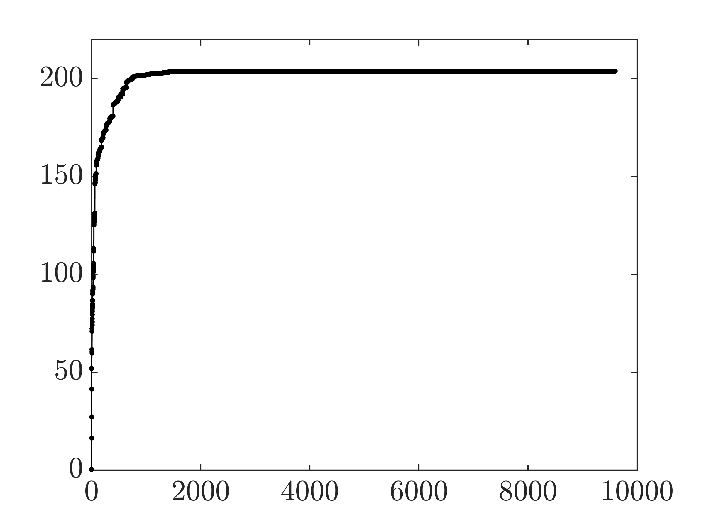
Refer to caption
iteration
(a) Jd(Y1,Y2)subscript𝐽𝑑subscript𝑌1subscript𝑌2J_{d}(Y_{1},Y_{2})
Refer to caption
iteration
(b) ΔgapsubscriptΔgap\Delta_{\mathrm{gap}}
Refer to caption
iteration
(c) ΔpsubscriptΔp\Delta_{\mathrm{p}}
Figure 3: Performance of AMABBsubscriptAMABB\mathrm{AMA_{BB}} for the MSD system with 505050 masses, γ=2.2𝛾2.2\gamma=2.2, ϵ1=0.005subscriptitalic-ϵ10.005{\epsilon}_{1}=0.005, and ϵ2=0.05subscriptitalic-ϵ20.05{\epsilon}_{2}=0.05. (a) The dual objective function Jd(Y1,Y2)subscript𝐽𝑑subscript𝑌1subscript𝑌2J_{d}(Y_{1},Y_{2}) of (CC); (b) the duality gap, |Δgap|subscriptΔgap|\Delta_{\mathrm{gap}}|; and (c) the primal residual, ΔpsubscriptΔp\Delta_{\mathrm{p}}.

|JdJd(Y1k,Y2k)|/|Jd|superscriptsubscript𝐽𝑑subscript𝐽𝑑superscriptsubscript𝑌1𝑘superscriptsubscript𝑌2𝑘superscriptsubscript𝐽𝑑|J_{d}^{\star}-J_{d}(Y_{1}^{k},Y_{2}^{k})|/|J_{d}^{\star}|

Refer to caption
iteration
(a)
Refer to caption
solve time (seconds)
(b)
Figure 4: Convergence curves showing performance of ADMM (\circ) and AMA with (-) and without (\triangle) BB step-size initialization vs. (a) the number of iterations; and (b) solve times for the MSD system with 505050 masses and γ=2.2𝛾2.2\gamma=2.2. Here, Jdsuperscriptsubscript𝐽𝑑J_{d}^{\star} is the value of the optimal dual objective.
Refer to caption
(a) diag(Σpp)diagsubscriptΣ𝑝𝑝\mathrm{diag}(\Sigma_{pp}), diag(Xpp)diagsubscript𝑋𝑝𝑝\mathrm{diag}(X_{pp})
Refer to caption
(b) diag(Σvv)diagsubscriptΣ𝑣𝑣\mathrm{diag}(\Sigma_{vv}), diag(Xvv)diagsubscript𝑋𝑣𝑣\mathrm{diag}(X_{vv})
Figure 5: Diagonals of (a) position and (b) velocity covariances for the MSD system with 505050 masses; Solid black lines show diagonals of ΣxxsubscriptΣ𝑥𝑥\Sigma_{xx} and red circles mark solutions of optimization problem (CC).
Refer to caption
time
Figure 6: Time evolution of the variance of the MSD system’s state vector for twenty realizations of white-in-time forcing to (14b). The variance averaged over all simulations is marked by the thick black line.

For MSD system with 505050 masses and γ=2.2𝛾2.2\gamma=2.2, we now focus on the convergence of AMA. Figure 3a shows monotonic increase of the dual objective function. The absolute value of the duality gap |Δgap|subscriptΔgap|\Delta_{\mathrm{gap}}| and the primal residual ΔpsubscriptΔp\Delta_{\mathrm{p}} demonstrate convergence of our customized algorithm; see Figs. 3b and 3c. In addition, Fig. 4a shows that regular AMA converges linearly to the optimal solution and that AMA with BB step-size initialization outperforms both regular AMA and ADMM. Thus, heuristic step-size initialization can improve the theoretically-established convergence rate. Similar trends are observed when convergence curves are plotted as a function of time; see 4b. Finally, Fig. 5 demonstrates feasibility of the optimization problem (CC) and perfect recovery of the available diagonal elements of the covariance matrix.

For γ=2.2𝛾2.2\gamma=2.2, the spectrum of Z𝑍Z contains 505050 positive and 121212 negative eigenvalues. Based on Proposition 2, Z𝑍Z can be decomposed into BH+HB𝐵superscript𝐻𝐻superscript𝐵BH^{*}+HB^{*}, where B𝐵B has 505050 independent columns. In other words, the identified X𝑋X can be explained by driving the state-space model with 505050 stochastic inputs u𝑢u. The algorithm presented in Section III-B is used to decompose Z𝑍Z into BH+HB𝐵superscript𝐻𝐻superscript𝐵BH^{*}+HB^{*}. For the identified input matrix B𝐵B, the design parameter K𝐾K is then chosen to satisfy the optimality criterion described in Section II-C. This yields the optimal filter (14) that generates the stochastic input u𝑢u. We use this filter to validate our approach as explained next.

We conduct linear stochastic simulations of system (14b) with zero-mean unit variance input w𝑤w. Figure 6 shows the time evolution of the state variance of the MSD system. Since proper comparison requires ensemble-averaging, we have conducted twenty stochastic simulations with different realizations of the stochastic input w𝑤w to (14b). The variance, averaged over all simulations, is given by the thick black line. Even though the responses of individual simulations differ from each other, the average of twenty sample sets asymptotically approaches the correct steady-state variance.

The recovered covariance matrix of mass positions Xppsubscript𝑋𝑝𝑝X_{pp} resulting from the ensemble-averaged simulations of (14b) is shown in Fig. 7b. We note that (i) only diagonal elements of this matrix (marked by the black line) are used as data in the optimization problem (CC), and that (ii) the recovery of the off-diagonal elements is remarkably consistent. This is to be contrasted with typical matrix completion techniques that require incoherence in sampling entries of the covariance matrix. The key in our formulation of structured covariance completion is the Lyapunov-like structural constraint (2b) in (CC). Indeed, it is precisely this constraint that retains the relevance of the system dynamics and, thereby, the physics of the problem.
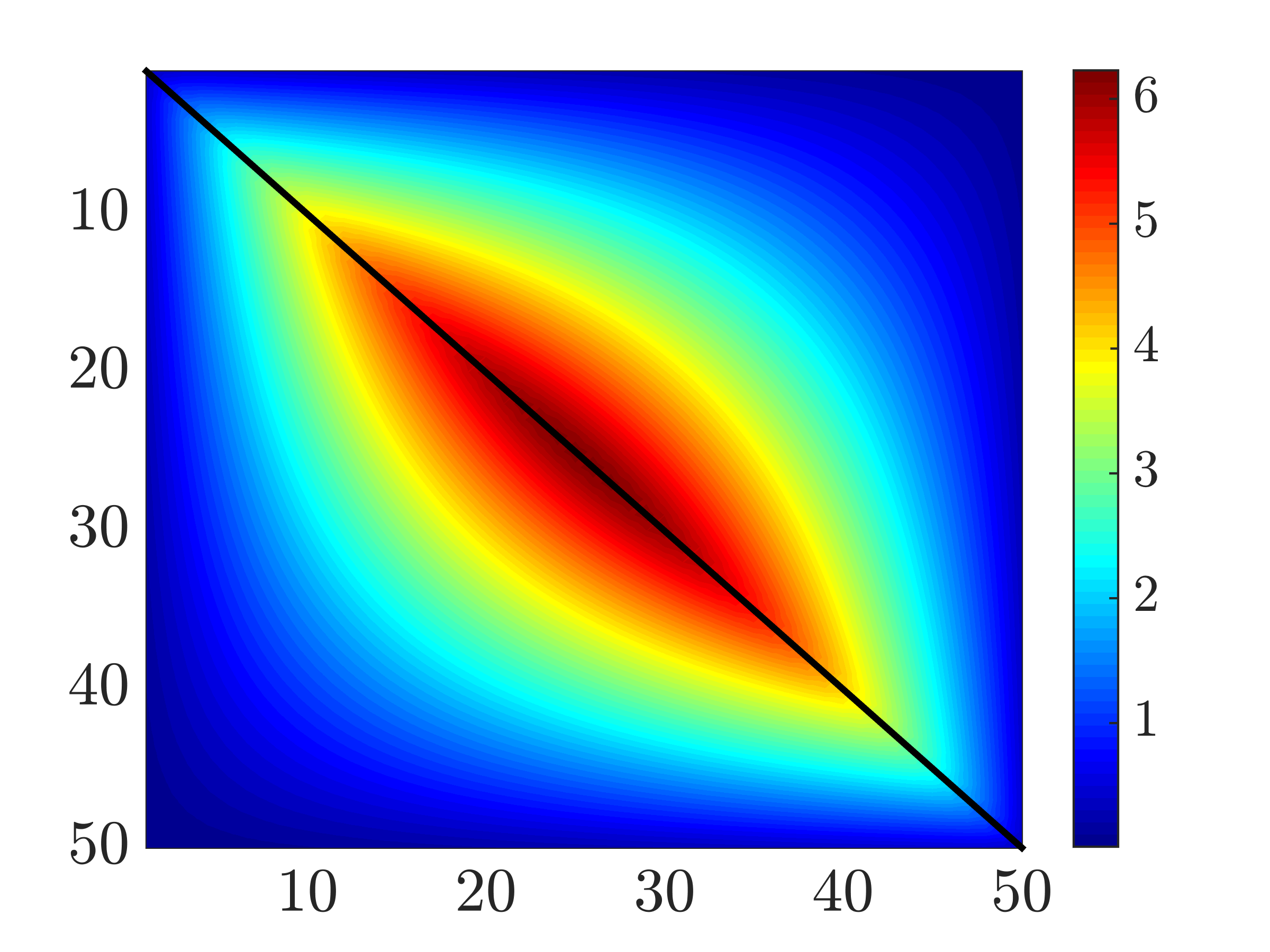
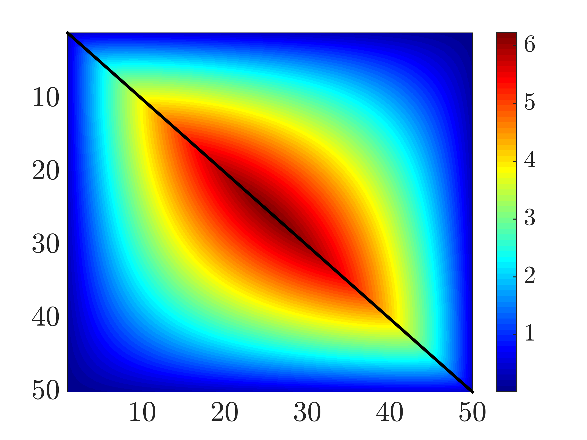
Refer to caption
(a) ΣppsubscriptΣ𝑝𝑝\Sigma_{pp}
Refer to caption
(b) Xppsubscript𝑋𝑝𝑝X_{pp}
Figure 7: The true covariance ΣppsubscriptΣ𝑝𝑝\Sigma_{pp} of the MSD system and the covariance Xppsubscript𝑋𝑝𝑝X_{pp} resulting from linear stochastic simulations of (14b). Available one-point correlations of the position of masses used in (CC) are marked by black lines along the main diagonals.
TABLE I: Solve times (in seconds) for different number of masses and γ=2.2𝛾2.2\gamma=2.2.
​​​ nn\mathrm{n} ​​​ ​​​ CVXCVX\mathrm{CVX} ​​​ ​​​ ADMMADMM\mathrm{ADMM} ​​​ ​​​ AMAAMA\mathrm{AMA} ​​​ ​​​ AMABBsubscriptAMABB\mathrm{AMA_{BB}} ​​​
​​​ 101010 ​​​ ​​​ 28.428.428.4 ​​​ ​​​ 222 ​​​ ​​​ 1.31.31.3 ​​​ ​​​ 0.50.50.5 ​​​
​​​ 202020 ​​​​ ​​​​ 419.7419.7419.7 ​​​​ ​​​​ 54.754.754.7 ​​​​ ​​​​ 30.730.730.7 ​​​​​ ​​​ 2.22.22.2 ​​​
​​​ 505050 ​​​​ ​​​​ 3442.93442.93442.9 ​​​​ ​​​​ 3796.73796.73796.7 ​​​​​ ​​​ 52.752.752.7 ​​​
​​​ 100100100 ​​​​ ​​​​ 407544075440754 ​​​​ ​​​​ 344203442034420 ​​​​​ ​​​ 5429.85429.85429.8 ​​​

VI Concluding remarks

We are interested in explaining partially known second-order statistics that originate from experimental measurements or simulations using stochastic linear models. This is motivated by the need for control-oriented models of systems with large number of degrees of freedom, e.g., turbulent fluid flows. In our setup, the linearized approximation of the dynamical generator is known whereas the nature and directionality of disturbances that can explain partially observed statistics are unknown. We thus formulate the problem of identifying appropriate stochastic input that can account for the observed statistics while being consistent with the linear dynamics.

This inverse problem is framed as convex optimization. To this end, nuclear norm minimization is utilized to identify noise parameters of low rank and to complete unavailable covariance data. Our formulation relies on drawing a connection between the rank of a certain matrix and the number of disturbance channels into the linear dynamics. An important contribution is the development of a customized alternating minimization algorithm (AMA) that efficiently solves covariance completion problems of large size. In fact, we show that our algorithm works as a proximal gradient on the dual problem and establish a sub-linear convergence rate for the fixed step-size. We also provide comparison with ADMM and demonstrate that AMA yields explicit updates of all optimization variables and a principled procedure for step-size selection. An additional contribution is the design of a class of linear filters that realize suitable colored-in-time excitation to account for the observed state statistics. These filters solve a non-standard stochastic realization problem with partial covariance information.

Broadly, our research program aims at developing a framework for control-oriented modeling of turbulent flows [41, 63, 64]. The present work represents a step in this direction in that it provides a theoretical and algorithmic approach for dealing with structured covariance completion problems of sizes that arise in fluids applications. In fact, we have recently employed our framework to model second-order statistics of turbulent flows via stochastically-forced linearized Navier-Stokes equations [64].

Appendix

Proof of Lemma 1

Without loss of generality, let us consider Z𝑍Z of the following form (see Section III-B for further justification)

Z= 2[Iπ000Iν0000].𝑍2delimited-[]subscript𝐼𝜋000subscript𝐼𝜈0000Z\;=\;2\left[\begin{array}[]{ccc}I_{\pi}&0&0\\ 0&-I_{\nu}&0\\ 0&0&0\end{array}\right]. (69)

Given any S𝑆S that satisfies Z=S+S𝑍𝑆superscript𝑆Z=S+S^{*} we can decompose it into

S=M+N𝑆𝑀𝑁S\;=\;M\,+\,N

with M𝑀M Hermitian and N𝑁N skew-Hermitian. It is easy to see that

M=12Z=[Iπ000Iν0000].𝑀12𝑍delimited-[]subscript𝐼𝜋000subscript𝐼𝜈0000M\;=\;\dfrac{1}{2}\,Z\;=\,\left[\begin{array}[]{ccc}I_{\pi}&0&0\\ 0&-I_{\nu}&0\\ 0&0&0\end{array}\right].

By partitioning N𝑁N as

N=[N11N12N13N21N22N23N31N32N33],𝑁delimited-[]subscript𝑁11subscript𝑁12subscript𝑁13subscript𝑁21subscript𝑁22subscript𝑁23subscript𝑁31subscript𝑁32subscript𝑁33N\;=\,\left[\begin{array}[]{ccc}N_{11}&N_{12}&N_{13}\\ N_{21}&N_{22}&N_{23}\\ N_{31}&N_{32}&N_{33}\end{array}\right],

we have

S=[Iπ+N11N12N13N21Iν+N22N23N31N32N33].𝑆delimited-[]subscript𝐼𝜋subscript𝑁11subscript𝑁12subscript𝑁13subscript𝑁21subscript𝐼𝜈subscript𝑁22subscript𝑁23subscript𝑁31subscript𝑁32subscript𝑁33S\;=\,\left[\begin{array}[]{ccc}I_{\pi}+N_{11}&N_{12}&N_{13}\\ N_{21}&-I_{\nu}+N_{22}&N_{23}\\ N_{31}&N_{32}&N_{33}\end{array}\right].

Clearly,

rank(S)rank(Iπ+N11).rank𝑆ranksubscript𝐼𝜋subscript𝑁11\operatorname*{rank}(S)\;\geq\;\operatorname*{rank}(I_{\pi}+N_{11}).

Since N11subscript𝑁11N_{11} is skew-Hermitian, all its eigenvalues are on the imaginary axis. This implies that all the eigenvalues of Iπ+N11subscript𝐼𝜋subscript𝑁11I_{\pi}+N_{11} have real part 1 and therefore Iπ+N11subscript𝐼𝜋subscript𝑁11I_{\pi}+N_{11} is a full rank matrix. Hence, we have

rank(S)rank(Iπ+N11)=π(Z)rank𝑆ranksubscript𝐼𝜋subscript𝑁11𝜋𝑍\operatorname*{rank}(S)\;\geq\;\operatorname*{rank}(I_{\pi}+N_{11})\;=\;\pi(Z)

which completes the proof.

Proof of Proposition 2

The inequality

min{rank(S)|Z=S+S}max{π(Z),ν(Z)}conditionalrank𝑆𝑍𝑆superscript𝑆𝜋𝑍𝜈𝑍\min\{\operatorname*{rank}(S)~{}|~{}Z\,=\,S+S^{*}\}\;\geq\;\max\{\pi(Z),\nu(Z)\}

follows from Lemma 1. To establish the proposition we need to show that the bounds are tight, i.e.,

min{rank(S)|Z=S+S}max{π(Z),ν(Z)}.conditionalrank𝑆𝑍𝑆superscript𝑆𝜋𝑍𝜈𝑍\min\{\operatorname*{rank}(S)~{}|~{}Z\,=\,S+S^{*}\}\;\leq\;\max\{\pi(Z),\nu(Z)\}.

Given Z𝑍Z in (69), for π(Z)ν(Z)𝜋𝑍𝜈𝑍\pi(Z)\leq\nu(Z), Z𝑍Z can be written as

Z= 2[Iπ0000Iπ0000Iνπ00000].𝑍2delimited-[]subscript𝐼𝜋0000subscript𝐼𝜋0000subscript𝐼𝜈𝜋00000\displaystyle Z\;=\;2\left[\begin{array}[]{cccc}I_{\pi}&0&0&0\\ 0&-I_{\pi}&0&0\\ 0&0&-I_{\nu-\pi}&0\\ 0&0&0&0\end{array}\right]. (74)

By selecting S𝑆S in the form (20) we conclude that

rank(S)rank𝑆\displaystyle\operatorname*{rank}(S) =\displaystyle\!\!=\!\! rank([IπIπIπIπ])+rank(Iνπ)rankdelimited-[]subscript𝐼𝜋subscript𝐼𝜋subscript𝐼𝜋subscript𝐼𝜋ranksubscript𝐼𝜈𝜋\displaystyle\operatorname*{rank}(\left[\begin{array}[]{cc}I_{\pi}&-I_{\pi}\\ I_{\pi}&-I_{\pi}\end{array}\right])\;+\;\operatorname*{rank}(-I_{\nu-\pi})
=\displaystyle\!\!=\!\! π(Z)+ν(Z)π(Z)=ν(Z).𝜋𝑍𝜈𝑍𝜋𝑍𝜈𝑍\displaystyle\pi(Z)\,+\,\nu(Z)\,-\,\pi(Z)\;=\;\nu(Z).

Therefore

min{rank(S)|Z=S+S}ν(Z).conditionalrank𝑆𝑍𝑆superscript𝑆𝜈𝑍\min\{\operatorname*{rank}(S)~{}|~{}Z\,=\,S+S^{*}\}\;\leq\;\nu(Z).

Similarly, for the case π(Z)>ν(Z)𝜋𝑍𝜈𝑍\pi(Z)>\nu(Z),

min{rank(S)|Z=S+S}π(Z).conditionalrank𝑆𝑍𝑆superscript𝑆𝜋𝑍\min\{\operatorname*{rank}(S)~{}|~{}Z\,=\,S+S^{*}\}\;\leq\;\pi(Z).

Hence,

min{rank(S)|Z=S+S}max{π(Z),ν(Z)}conditionalrank𝑆𝑍𝑆superscript𝑆𝜋𝑍𝜈𝑍\min\{\operatorname*{rank}(S)~{}|~{}Z\,=\,S+S^{*}\}\;\leq\;\max\{\pi(Z),\nu(Z)\}

which completes the proof.

Proof of Lemma 2

The second-order approximation of logdet𝒜(Y)logdetsuperscript𝒜𝑌\operatorname*{log\,det}{\cal A}^{\dagger}(Y) yields

logdet𝒜(Y+ΔY)=logdet𝒜(Y)+trace(𝒜(Y)1𝒜(ΔY))12trace(𝒜(Y)1𝒜(ΔY)𝒜(Y)1𝒜(ΔY))+O(ΔYF2).logdetsuperscript𝒜𝑌Δ𝑌logdetsuperscript𝒜𝑌limit-fromtracesuperscript𝒜superscript𝑌1superscript𝒜Δ𝑌missing-subexpressionmissing-subexpression12tracesuperscript𝒜superscript𝑌1superscript𝒜Δ𝑌superscript𝒜superscript𝑌1superscript𝒜Δ𝑌𝑂superscriptsubscriptnormΔ𝑌𝐹2\begin{array}[]{rcl}\operatorname*{log\,det}{\cal A}^{\dagger}(Y+\Delta Y)&\!\!=\!\!&\operatorname*{log\,det}{\cal A}^{\dagger}(Y)\,+\,\mathrm{trace}\left({\cal A}^{\dagger}(Y)^{-1}{\cal A}^{\dagger}(\Delta Y)\right)\;-\\[4.26773pt] &\!\!\!\!&\dfrac{1}{2}\,\mathrm{trace}\left({\cal A}^{\dagger}(Y)^{-1}{\cal A}^{\dagger}(\Delta Y)\,{\cal A}^{\dagger}(Y)^{-1}{\cal A}^{\dagger}(\Delta Y)\right)\,+\,O(\|\Delta Y\|_{F}^{2}).\end{array}

To show Lipschitz continuity of the gradient it is sufficient to show that the approximation to the Hessian is bounded by the Lipschitz constant L𝐿L, i.e.,

trace(𝒜(Y)1𝒜(ΔY)𝒜(Y)1𝒜(ΔY))LΔYF2.tracesuperscript𝒜superscript𝑌1superscript𝒜Δ𝑌superscript𝒜superscript𝑌1superscript𝒜Δ𝑌𝐿superscriptsubscriptnormΔ𝑌𝐹2\mathrm{trace}\left({\cal A}^{\dagger}(Y)^{-1}{\cal A}^{\dagger}(\Delta Y)\,{\cal A}^{\dagger}(Y)^{-1}{\cal A}^{\dagger}(\Delta Y)\right)\;\leq\;L\,\|\Delta Y\|_{F}^{2}.

From the left-hand-side we have

trace(𝒜(Y)1𝒜(ΔY)𝒜(Y)1𝒜(ΔY))=trace(𝒜(Y)12𝒜(ΔY)𝒜(Y)1𝒜(ΔY)𝒜(Y)12)1αtrace(𝒜(Y)12𝒜(ΔY)𝒜(ΔY)𝒜(Y)12)=1αtrace(𝒜(ΔY)𝒜(Y)1𝒜(ΔY))1α2trace(𝒜(ΔY)𝒜(ΔY))σmax2(𝒜)α2ΔYF2.tracesuperscript𝒜superscript𝑌1superscript𝒜Δ𝑌superscript𝒜superscript𝑌1superscript𝒜Δ𝑌tracesuperscript𝒜superscript𝑌12superscript𝒜Δ𝑌superscript𝒜superscript𝑌1superscript𝒜Δ𝑌superscript𝒜superscript𝑌12missing-subexpression1𝛼tracesuperscript𝒜superscript𝑌12superscript𝒜Δ𝑌superscript𝒜Δ𝑌superscript𝒜superscript𝑌12missing-subexpression1𝛼tracesuperscript𝒜Δ𝑌superscript𝒜superscript𝑌1superscript𝒜Δ𝑌missing-subexpression1superscript𝛼2tracesuperscript𝒜Δ𝑌superscript𝒜Δ𝑌missing-subexpressionsubscriptsuperscript𝜎2superscript𝒜superscript𝛼2superscriptsubscriptnormΔ𝑌𝐹2\begin{array}[]{rcl}\mathrm{trace}\left({\cal A}^{\dagger}(Y)^{-1}{\cal A}^{\dagger}(\Delta Y)\,{\cal A}^{\dagger}(Y)^{-1}{\cal A}^{\dagger}(\Delta Y)\right)&\!\!=\!\!&\mathrm{trace}\left({\cal A}^{\dagger}(Y)^{-\frac{1}{2}}\,{\cal A}^{\dagger}(\Delta Y)\,{\cal A}^{\dagger}(Y)^{-1}{\cal A}^{\dagger}(\Delta Y)\,{\cal A}^{\dagger}(Y)^{-\frac{1}{2}}\right)\\[5.69046pt] &\!\!\leq\!\!&\dfrac{1}{\alpha}\,\mathrm{trace}\left({\cal A}^{\dagger}(Y)^{-\frac{1}{2}}\,{\cal A}^{\dagger}(\Delta Y)\,{\cal A}^{\dagger}(\Delta Y)\,{\cal A}^{\dagger}(Y)^{-\frac{1}{2}}\right)\\[5.69046pt] &\!\!=\!\!&\dfrac{1}{\alpha}\,\mathrm{trace}\left({\cal A}^{\dagger}(\Delta Y)\,{\cal A}^{\dagger}(Y)^{-1}{\cal A}^{\dagger}(\Delta Y)\right)\\[5.69046pt] &\!\!\leq\!\!&\dfrac{1}{\alpha^{2}}\,\mathrm{trace}\left({\cal A}^{\dagger}(\Delta Y)\,{\cal A}^{\dagger}(\Delta Y)\right)\\[5.69046pt] &\!\!\leq\!\!&\dfrac{\sigma^{2}_{\max}({\cal A}^{\dagger})}{\alpha^{2}}\,\|\Delta Y\|_{F}^{2}.\end{array}

Here, we have repeatedly utilized the fact that 𝒜(Y)1superscript𝒜superscript𝑌1{\cal A}^{\dagger}(Y)^{-1} is a positive-definite matrix and that Y𝒟αβ𝑌subscript𝒟𝛼𝛽Y\in{\cal D}_{\alpha\beta}. This completes the proof.

Proof of Lemma 3

We begin by substituting the expressions for Y1+superscriptsubscript𝑌1Y_{1}^{+}, Y2+superscriptsubscript𝑌2Y_{2}^{+}, Y¯1subscript¯𝑌1\bar{Y}_{1}, and Y¯2subscript¯𝑌2\bar{Y}_{2}. Utilizing the non-expansive property of the proximal operator 𝒯γsubscript𝒯𝛾\mathcal{T}_{\gamma} [65] we have

Y1+Y¯1F=𝒯γ(Y1+ρ𝒜1(𝒜(Y1,Y2)1))𝒯γ(Y¯1+ρ𝒜1(𝒜(Y¯1,Y¯2)1))FY1+ρ𝒜1(𝒜(Y1,Y2)1)Y¯1ρ𝒜1(𝒜(Y¯1,Y¯2)1)FY2+Y¯2F=Y2+ρ(𝒜2(𝒜(Y1,Y2)1)G)Y¯2ρ(𝒜2(𝒜(Y¯1,Y¯2)1)G)F,subscriptnormsuperscriptsubscript𝑌1subscript¯𝑌1𝐹subscriptnormsubscript𝒯𝛾subscript𝑌1𝜌subscript𝒜1superscript𝒜superscriptsubscript𝑌1subscript𝑌21subscript𝒯𝛾subscript¯𝑌1𝜌subscript𝒜1superscript𝒜superscriptsubscript¯𝑌1subscript¯𝑌21𝐹missing-subexpressionsubscriptnormsubscript𝑌1𝜌subscript𝒜1superscript𝒜superscriptsubscript𝑌1subscript𝑌21subscript¯𝑌1𝜌subscript𝒜1superscript𝒜superscriptsubscript¯𝑌1subscript¯𝑌21𝐹subscriptnormsuperscriptsubscript𝑌2subscript¯𝑌2𝐹subscriptnormsubscript𝑌2𝜌subscript𝒜2superscript𝒜superscriptsubscript𝑌1subscript𝑌21𝐺subscript¯𝑌2𝜌subscript𝒜2superscript𝒜superscriptsubscript¯𝑌1subscript¯𝑌21𝐺𝐹\begin{array}[]{rcl}\|Y_{1}^{+}-\,\bar{Y}_{1}\|_{F}&\!\!=\!\!&||\;\mathcal{T}_{\gamma}\left(Y_{1}\,+\,\rho\,{\cal A}_{1}({\cal A}^{\dagger}(Y_{1},Y_{2})^{-1})\right)\,-\,\mathcal{T}_{\gamma}\left(\bar{Y}_{1}\,+\,\rho\,{\cal A}_{1}({\cal A}^{\dagger}(\bar{Y}_{1},\bar{Y}_{2})^{-1})\right)||_{F}\\[4.26773pt] &\!\!\leq\!\!&||\;Y_{1}\,+\,\rho\,{\cal A}_{1}({\cal A}^{\dagger}(Y_{1},Y_{2})^{-1})\,-\,\bar{Y}_{1}\,-\,\rho\,{\cal A}_{1}({\cal A}^{\dagger}(\bar{Y}_{1},\bar{Y}_{2})^{-1})\,||_{F}\\[7.11317pt] \|Y_{2}^{+}-\,\bar{Y}_{2}\|_{F}&\!\!=\!\!&||\;Y_{2}\,+\,\rho\left({\cal A}_{2}({\cal A}^{\dagger}(Y_{1},Y_{2})^{-1})\,-\,G\right)\,-\,\bar{Y}_{2}\,-\,\rho\left({\cal A}_{2}({\cal A}^{\dagger}(\bar{Y}_{1},\bar{Y}_{2})^{-1})\,-\,G\right)||_{F},\end{array}

from which we obtain

Y+Y¯Fhρ(Y)hρ(Y¯)F,subscriptnormsuperscript𝑌¯𝑌𝐹subscriptnormsubscript𝜌𝑌subscript𝜌¯𝑌𝐹\|Y^{+}-\,\bar{Y}\|_{F}\;\leq\;\|h_{\rho}(Y)\,-\,h_{\rho}(\bar{Y})\|_{F},

where

hρ(Y)=Y+ρ𝒜(𝒜(Y)1).subscript𝜌𝑌𝑌𝜌𝒜superscript𝒜superscript𝑌1h_{\rho}(Y)\;=\;Y\;+\;\rho\,{\cal A}\left({\cal A}^{\dagger}(Y)^{-1}\right).

The first order approximation of the linear map hρsubscript𝜌h_{\rho} gives

hρ(Y+ΔY)hρ(Y)ΔYρ𝒜(𝒜(Y)1𝒜(ΔY)𝒜(Y)1).subscript𝜌𝑌Δ𝑌subscript𝜌𝑌Δ𝑌𝜌𝒜superscript𝒜superscript𝑌1superscript𝒜Δ𝑌superscript𝒜superscript𝑌1\begin{array}[]{l}h_{\rho}(Y+\Delta Y)\,-\,h_{\rho}(Y)\;\approx\;\Delta Y\,-\,\rho\,{\cal A}\left({\cal A}^{\dagger}(Y)^{-1}{\cal A}^{\dagger}(\Delta Y){\cal A}^{\dagger}(Y)^{-1}\right).\end{array}

From this we conclude that its Jacobian at Y𝑌Y is 1absent1\leq 1 if

𝒜(𝒜(Y)1𝒜(ΔY)𝒜(Y)1),ΔY 0,𝒜superscript𝒜superscript𝑌1superscript𝒜Δ𝑌superscript𝒜superscript𝑌1Δ𝑌 0\left<{\cal A}\left({\cal A}^{\dagger}(Y)^{-1}{\cal A}^{\dagger}(\Delta Y){\cal A}^{\dagger}(Y)^{-1}\right),\Delta Y\right>\;\geq\;0,

and the step-size 0<ρ2α4β2σmax2(𝒜)0𝜌2superscript𝛼4superscript𝛽2subscriptsuperscript𝜎2𝒜0<\rho\leq\dfrac{2\,\alpha^{4}}{\beta^{2}\,\sigma^{2}_{\max}({\cal A})} satisfies

ρ2𝒜(𝒜(Y)1𝒜(ΔY)𝒜(Y)1)F2𝒜(𝒜(Y)1𝒜(ΔY)𝒜(Y)1),ΔY𝜌2superscriptsubscriptnorm𝒜superscript𝒜superscript𝑌1superscript𝒜Δ𝑌superscript𝒜superscript𝑌1𝐹2𝒜superscript𝒜superscript𝑌1superscript𝒜Δ𝑌superscript𝒜superscript𝑌1Δ𝑌\dfrac{\rho}{2}\,\|{\cal A}\left({\cal A}^{\dagger}(Y)^{-1}{\cal A}^{\dagger}(\Delta Y)\,{\cal A}^{\dagger}(Y)^{-1}\right)\|_{F}^{2}\;\leq\;\left<{\cal A}\left({\cal A}^{\dagger}(Y)^{-1}{\cal A}^{\dagger}(\Delta Y)\,{\cal A}^{\dagger}(Y)^{-1}\right),\Delta Y\right>

for any perturbation ΔYΔ𝑌\Delta Y. The former follows from

𝒜(Y)1𝒜(ΔY)𝒜(Y)1,𝒜(ΔY)=trace(𝒜(Y)1𝒜(ΔY)𝒜(Y)1𝒜(ΔY))=trace(𝒜(Y)1/2𝒜(ΔY)𝒜(Y)1𝒜(ΔY)𝒜(Y)1/2),superscript𝒜superscript𝑌1superscript𝒜Δ𝑌superscript𝒜superscript𝑌1superscript𝒜Δ𝑌tracesuperscript𝒜superscript𝑌1superscript𝒜Δ𝑌superscript𝒜superscript𝑌1superscript𝒜Δ𝑌missing-subexpressiontracesuperscript𝒜superscript𝑌12superscript𝒜Δ𝑌superscript𝒜superscript𝑌1superscript𝒜Δ𝑌superscript𝒜superscript𝑌12\begin{array}[]{rcl}\left<{\cal A}^{\dagger}(Y)^{-1}{\cal A}^{\dagger}(\Delta Y){\cal A}^{\dagger}(Y)^{-1},{\cal A}^{\dagger}(\Delta Y)\right>&\!\!=\!\!&\mathrm{trace}\,({\cal A}^{\dagger}(Y)^{-1}{\cal A}^{\dagger}(\Delta Y)\,{\cal A}^{\dagger}(Y)^{-1}{\cal A}^{\dagger}(\Delta Y))\\[4.26773pt] &\!\!=\!\!&\mathrm{trace}\,({\cal A}^{\dagger}(Y)^{-1/2}{\cal A}^{\dagger}(\Delta Y){\cal A}^{\dagger}(Y)^{-1}{\cal A}^{\dagger}(\Delta Y){\cal A}^{\dagger}(Y)^{-1/2}),\end{array}

and the latter follows from

ρ2𝒜(𝒜(Y)1𝒜(ΔY)𝒜(Y)1)F2ρσmax2(𝒜)2𝒜(Y)1𝒜(ΔY)𝒜(Y)1F2ρσmax2(𝒜)2α4𝒜(ΔY)F2ρβ2σmax2(𝒜)2α4𝒜(Y)1𝒜(ΔY)𝒜(Y)1,𝒜(ΔY)=ρβ2σmax2(𝒜)2α4𝒜(𝒜(Y)1𝒜(ΔY)𝒜(Y)1),ΔY𝒜(𝒜(Y)1𝒜(ΔY)𝒜(Y)1),ΔY.𝜌2superscriptsubscriptnorm𝒜superscript𝒜superscript𝑌1superscript𝒜Δ𝑌superscript𝒜superscript𝑌1𝐹2𝜌subscriptsuperscript𝜎2𝒜2superscriptsubscriptnormsuperscript𝒜superscript𝑌1superscript𝒜Δ𝑌superscript𝒜superscript𝑌1𝐹2missing-subexpression𝜌subscriptsuperscript𝜎2𝒜2superscript𝛼4superscriptsubscriptnormsuperscript𝒜Δ𝑌𝐹2missing-subexpression𝜌superscript𝛽2subscriptsuperscript𝜎2𝒜2superscript𝛼4superscript𝒜superscript𝑌1superscript𝒜Δ𝑌superscript𝒜superscript𝑌1superscript𝒜Δ𝑌missing-subexpression𝜌superscript𝛽2subscriptsuperscript𝜎2𝒜2superscript𝛼4𝒜superscript𝒜superscript𝑌1superscript𝒜Δ𝑌superscript𝒜superscript𝑌1Δ𝑌missing-subexpression𝒜superscript𝒜superscript𝑌1superscript𝒜Δ𝑌superscript𝒜superscript𝑌1Δ𝑌\begin{array}[]{rcl}\dfrac{\rho}{2}\,\|{\cal A}\left({\cal A}^{\dagger}(Y)^{-1}{\cal A}^{\dagger}(\Delta Y)\,{\cal A}^{\dagger}(Y)^{-1}\right)\|_{F}^{2}&\!\!\leq\!\!&\dfrac{\rho\,\sigma^{2}_{\max}({\cal A})}{2}\,\|{\cal A}^{\dagger}(Y)^{-1}{\cal A}^{\dagger}(\Delta Y)\,{\cal A}^{\dagger}(Y)^{-1}\|_{F}^{2}\\[7.11317pt] &\!\!\leq\!\!&\dfrac{\rho\,\sigma^{2}_{\max}({\cal A})}{2\,\alpha^{4}}\,\|{\cal A}^{\dagger}(\Delta Y)\|_{F}^{2}\\[7.11317pt] &\!\!\leq\!\!&\dfrac{\rho\,\beta^{2}\,\sigma^{2}_{\max}({\cal A})}{2\,\alpha^{4}}\,\left<{\cal A}^{\dagger}(Y)^{-1}{\cal A}^{\dagger}(\Delta Y){\cal A}^{\dagger}(Y)^{-1},{\cal A}^{\dagger}(\Delta Y)\right>\\[7.11317pt] &\!\!=\!\!&\dfrac{\rho\,\beta^{2}\,\sigma^{2}_{\max}({\cal A})}{2\,\alpha^{4}}\,\left<{\cal A}\left({\cal A}^{\dagger}(Y)^{-1}{\cal A}^{\dagger}(\Delta Y){\cal A}^{\dagger}(Y)^{-1}\right),\Delta Y\right>\\[7.11317pt] &\!\!\leq\!\!&\left<{\cal A}\left({\cal A}^{\dagger}(Y)^{-1}{\cal A}^{\dagger}(\Delta Y){\cal A}^{\dagger}(Y)^{-1}\right),\Delta Y\right>.\end{array}

Thus, we conclude Jhρ(Y)1subscript𝐽subscript𝜌𝑌1J_{h_{\rho}}(Y)\leq 1 for all Y𝒟αβ𝑌subscript𝒟𝛼𝛽Y\in{\cal D}_{\alpha\beta}. Finally, from the mean value theorem, we have

Y+Y¯Fhρ(Y)hρ(Y¯)Fsupδ[0,1]Jhρ(Yδ)YY¯F,YY¯Fsubscriptnormsuperscript𝑌¯𝑌𝐹subscriptnormsubscript𝜌𝑌subscript𝜌¯𝑌𝐹missing-subexpressionsubscriptsupremum𝛿01subscript𝐽subscript𝜌subscript𝑌𝛿subscriptnorm𝑌¯𝑌𝐹missing-subexpressionsubscriptnorm𝑌¯𝑌𝐹\begin{array}[]{rcl}\|Y^{+}-\,\bar{Y}\|_{F}&\!\!\leq\!\!&\|h_{\rho}(Y)\,-\,h_{\rho}(\bar{Y})\|_{F}\\[4.26773pt] &\!\!\leq\!\!&\sup\limits_{\delta\,\in\,[0,1]}\,J_{h_{\rho}}(Y_{\delta})\,\|Y\,-\,\bar{Y}\|_{F},\\[4.26773pt] &\!\!\leq\!\!&\|Y\,-\,\bar{Y}\|_{F}\end{array}

where Yδ=δY+(1δ)Y¯𝒟αβsubscript𝑌𝛿𝛿𝑌1𝛿¯𝑌subscript𝒟𝛼𝛽Y_{\delta}=\delta\,Y+(1-\delta)\,\bar{Y}\in{\cal D}_{\alpha\beta}. This completes the proof.

Proof of Lemma 4

We first show that

αI𝒜(Y0)βI.precedes-or-equals𝛼𝐼superscript𝒜superscript𝑌0precedes-or-equals𝛽𝐼\alpha I\,\preceq\,{\cal A}^{\dagger}(Y^{0})\,\preceq\,\beta I.

The upper bound follows from

𝒜(Y0)2subscriptnormsuperscript𝒜superscript𝑌02\displaystyle\|{\cal A}^{\dagger}(Y^{0})\|_{2} =\displaystyle= 𝒜(Y0)2𝒜(Y¯)2+𝒜(Y¯)2subscriptnormsuperscript𝒜superscript𝑌02subscriptnormsuperscript𝒜¯𝑌2subscriptnormsuperscript𝒜¯𝑌2\displaystyle\|{\cal A}^{\dagger}(Y^{0})\|_{2}-\|{\cal A}^{\dagger}(\bar{Y})\|_{2}+\|{\cal A}^{\dagger}(\bar{Y})\|_{2}
\displaystyle\leq 𝒜(Y0)𝒜(Y¯)2+𝒜(Y¯)2subscriptnormsuperscript𝒜superscript𝑌0superscript𝒜¯𝑌2subscriptnormsuperscript𝒜¯𝑌2\displaystyle\|{\cal A}^{\dagger}(Y^{0})-{\cal A}^{\dagger}(\bar{Y})\|_{2}+\|{\cal A}^{\dagger}(\bar{Y})\|_{2}
\displaystyle\leq 𝒜(Y0)𝒜(Y¯)F+𝒜(Y¯)2subscriptnormsuperscript𝒜superscript𝑌0superscript𝒜¯𝑌𝐹subscriptnormsuperscript𝒜¯𝑌2\displaystyle\|{\cal A}^{\dagger}(Y^{0})-{\cal A}^{\dagger}(\bar{Y})\|_{F}+\|{\cal A}^{\dagger}(\bar{Y})\|_{2}
\displaystyle\leq σmax(𝒜)Y0Y¯F+𝒜(Y¯)2=β.subscript𝜎superscript𝒜subscriptnormsuperscript𝑌0¯𝑌𝐹subscriptnormsuperscript𝒜¯𝑌2𝛽\displaystyle\sigma_{\max}({\cal A}^{\dagger})\|Y^{0}-\bar{Y}\|_{F}+\|{\cal A}^{\dagger}(\bar{Y})\|_{2}\;=\;\beta.

To see the lower bound, note that for any Xn𝑋superscript𝑛X\in\mathbb{H}^{n},

1nXFX2XF.1𝑛subscriptnorm𝑋𝐹subscriptnorm𝑋2subscriptnorm𝑋𝐹\dfrac{1}{\sqrt{n}}\,\|X\|_{F}\;\leq\;\|X\|_{2}\;\leq\;\|X\|_{F}. (78)

Using this property and the dual constraint Y102γsubscriptnormsuperscriptsubscript𝑌102𝛾\|Y_{1}^{0}\|_{2}\leq\gamma we have

𝒜1(Y10)2𝒜1(Y10)Fσmax(𝒜1)Y10Fnσmax(𝒜1)Y102γnσmax(𝒜1).subscriptnormsuperscriptsubscript𝒜1superscriptsubscript𝑌102subscriptnormsuperscriptsubscript𝒜1superscriptsubscript𝑌10𝐹subscript𝜎superscriptsubscript𝒜1subscriptnormsuperscriptsubscript𝑌10𝐹𝑛subscript𝜎superscriptsubscript𝒜1subscriptnormsuperscriptsubscript𝑌102𝛾𝑛subscript𝜎superscriptsubscript𝒜1\|{\cal A}_{1}^{\dagger}(Y_{1}^{0})\|_{2}\;\leq\;\|{\cal A}_{1}^{\dagger}(Y_{1}^{0})\|_{F}\;\leq\;\sigma_{\max}({\cal A}_{1}^{\dagger})\,\|Y_{1}^{0}\|_{F}\;\leq\;\sqrt{n}\,\sigma_{\max}({\cal A}_{1}^{\dagger})\,\|Y_{1}^{0}\|_{2}\;\leq\;\gamma\,\sqrt{n}\,\sigma_{\max}({\cal A}_{1}^{\dagger}).

Since 𝒜1(Y10)+𝒜2(Y20)0succeedssuperscriptsubscript𝒜1superscriptsubscript𝑌10superscriptsubscript𝒜2superscriptsubscript𝑌200{\cal A}_{1}^{\dagger}(Y_{1}^{0})+{\cal A}_{2}^{\dagger}(Y_{2}^{0})\succ 0, we also have

𝒜2(Y20)γnσmax(𝒜1)I.succeeds-or-equalssuperscriptsubscript𝒜2superscriptsubscript𝑌20𝛾𝑛subscript𝜎superscriptsubscript𝒜1𝐼{\cal A}_{2}^{\dagger}(Y_{2}^{0})\;\succeq\;-\,\gamma\,\sqrt{n}\,\sigma_{\max}({\cal A}_{1}^{\dagger})\,I.

Noting G=𝒜2(X¯)𝐺subscript𝒜2¯𝑋G={\cal A}_{2}(\bar{X}) for the optimal solution X¯0succeeds¯𝑋0\bar{X}\succ 0, we obtain

G,Y20=𝒜2(X¯),Y20=X¯,𝒜2(Y20)γnσmax(𝒜1)trace(X¯).𝐺superscriptsubscript𝑌20subscript𝒜2¯𝑋superscriptsubscript𝑌20¯𝑋superscriptsubscript𝒜2superscriptsubscript𝑌20missing-subexpression𝛾𝑛subscript𝜎superscriptsubscript𝒜1trace¯𝑋\begin{array}[]{rcl}\left<G,Y_{2}^{0}\right>\;=\;\left<{\cal A}_{2}(\bar{X}),Y_{2}^{0}\right>&\!\!=\!\!&\left<\bar{X},{\cal A}_{2}^{\dagger}(Y_{2}^{0})\right>\\[4.26773pt] &\!\!\geq\!\!&-\,\gamma\,\sqrt{n}\,\sigma_{\max}({\cal A}_{1}^{\dagger})\,\mathrm{trace}(\bar{X}).\end{array} (79)

Let a=λmin(𝒜(Y0))𝑎subscript𝜆superscript𝒜superscript𝑌0a=\lambda_{\min}({\cal A}^{\dagger}(Y^{0})). Since β𝛽\beta gives a bound on the largest eigenvalue of 𝒜(Y0)superscript𝒜superscript𝑌0{\cal A}^{\dagger}(Y^{0}), we have

logdet𝒜(Y0)log(a)+(n1)log(β)logdetsuperscript𝒜superscript𝑌0𝑎𝑛1𝛽\operatorname*{log\,det}{\cal A}^{\dagger}(Y^{0})\;\leq\;\log(a)\,+\,(n-1)\log(\beta)

Combining this and

logdet𝒜(Y0)logdet𝒜(Y0)G,Y20+G,Y20logdet𝒜(Y0)G,Y20γnσmax(𝒜1)trace(X¯).logdetsuperscript𝒜superscript𝑌0logdetsuperscript𝒜superscript𝑌0𝐺superscriptsubscript𝑌20𝐺superscriptsubscript𝑌20missing-subexpressionlogdetsuperscript𝒜superscript𝑌0𝐺superscriptsubscript𝑌20𝛾𝑛subscript𝜎superscriptsubscript𝒜1trace¯𝑋\begin{array}[]{rcl}\operatorname*{log\,det}{\cal A}^{\dagger}(Y^{0})&\!\!\geq\!\!&\operatorname*{log\,det}{\cal A}^{\dagger}(Y^{0})\,-\,\left<G,Y_{2}^{0}\right>\,+\,\left<G,Y_{2}^{0}\right>\\[4.26773pt] &\!\!\geq\!\!&\operatorname*{log\,det}{\cal A}^{\dagger}(Y^{0})\,-\,\left<G,Y_{2}^{0}\right>\,-\,\gamma\,\sqrt{n}\,\sigma_{\max}({\cal A}_{1}^{\dagger})\,\mathrm{trace}(\bar{X}).\end{array}

gives λmin(𝒜(Y0))=aαsubscript𝜆superscript𝒜superscript𝑌0𝑎𝛼\lambda_{\min}({\cal A}^{\dagger}(Y^{0}))=a\geq\alpha.

The proof of αI𝒜(Yk)βIprecedes-or-equals𝛼𝐼superscript𝒜superscript𝑌𝑘precedes-or-equals𝛽𝐼\alpha I\preceq{\cal A}^{\dagger}(Y^{k})\preceq\beta I for k>0𝑘0k>0 follows similar lines. We use inductive argument to prove this. Assume that αI𝒜(Y)βIprecedes-or-equals𝛼𝐼superscript𝒜superscript𝑌precedes-or-equals𝛽𝐼\alpha I\preceq{\cal A}^{\dagger}(Y^{\ell})\preceq\beta I holds for all 0k10𝑘10\leq\ell\leq k-1. For the upper bound, we have

𝒜(Yk)2=𝒜(Yk)2𝒜(Y¯)2+𝒜(Y¯)2𝒜(Yk)𝒜(Y¯)F+𝒜(Y¯)2σmax(𝒜)YkY¯F+𝒜(Y¯)2.subscriptnormsuperscript𝒜superscript𝑌𝑘2subscriptnormsuperscript𝒜superscript𝑌𝑘2subscriptnormsuperscript𝒜¯𝑌2subscriptnormsuperscript𝒜¯𝑌2missing-subexpressionsubscriptnormsuperscript𝒜superscript𝑌𝑘superscript𝒜¯𝑌𝐹subscriptnormsuperscript𝒜¯𝑌2missing-subexpressionsubscript𝜎superscript𝒜subscriptnormsuperscript𝑌𝑘¯𝑌𝐹subscriptnormsuperscript𝒜¯𝑌2\begin{array}[]{rcl}\|{\cal A}^{\dagger}(Y^{k})\|_{2}&\!\!=\!\!&\|{\cal A}^{\dagger}(Y^{k})\|_{2}\;-\;\|{\cal A}^{\dagger}(\bar{Y})\|_{2}\;+\;\|{\cal A}^{\dagger}(\bar{Y})\|_{2}\\[4.26773pt] &\!\!\leq\!\!&\|{\cal A}^{\dagger}(Y^{k})\,-\,{\cal A}^{\dagger}(\bar{Y})\|_{F}\;+\;\|{\cal A}^{\dagger}(\bar{Y})\|_{2}\\[4.26773pt] &\!\!\leq\!\!&\sigma_{\max}({\cal A}^{\dagger})\,\|Y^{k}-\,\bar{Y}\|_{F}\;+\;\|{\cal A}^{\dagger}(\bar{Y})\|_{2}.\end{array}

By repeatedly applying Lemma 3 for YjY¯FYj1Y¯Fsubscriptnormsuperscript𝑌𝑗¯𝑌𝐹subscriptnormsuperscript𝑌𝑗1¯𝑌𝐹\|Y^{j}-\,\bar{Y}\|_{F}\leq\|Y^{j-1}-\,\bar{Y}\|_{F}, for all 1jk1𝑗𝑘1\leq j\leq k we have

𝒜(Yk)2σmax(𝒜)Y0Y¯F+𝒜(Y¯)2=β.subscriptnormsuperscript𝒜superscript𝑌𝑘2subscript𝜎superscript𝒜subscriptnormsuperscript𝑌0¯𝑌𝐹subscriptnormsuperscript𝒜¯𝑌2𝛽\displaystyle\|{\cal A}^{\dagger}(Y^{k})\|_{2}\;\leq\;\sigma_{\max}({\cal A}^{\dagger})\,\|Y^{0}-\,\bar{Y}\|_{F}\;+\;\|{\cal A}^{\dagger}(\bar{Y})\|_{2}\;=\;\beta.

To see the lower bound, note that (79) holds for all k0𝑘0k\geq 0, namely,

G,Y2k=𝒜2(X¯),Y2k=X¯,𝒜2(Y2k)γnσmax(𝒜1)trace(X¯),𝐺superscriptsubscript𝑌2𝑘subscript𝒜2¯𝑋superscriptsubscript𝑌2𝑘¯𝑋superscriptsubscript𝒜2superscriptsubscript𝑌2𝑘missing-subexpression𝛾𝑛subscript𝜎superscriptsubscript𝒜1trace¯𝑋\begin{array}[]{rcl}\left<G,Y_{2}^{k}\right>\;=\;\left<{\cal A}_{2}(\bar{X}),Y_{2}^{k}\right>&\!\!=\!\!&\left<\bar{X},{\cal A}_{2}^{\dagger}(Y_{2}^{k})\right>\\[4.26773pt] &\!\!\geq\!\!&-\,\gamma\,\sqrt{n}\,\sigma_{\max}({\cal A}_{1}^{\dagger})\,\mathrm{trace}(\bar{X}),\end{array} (80)

with the same argument. Let a=λmin(𝒜(Yk))𝑎subscript𝜆superscript𝒜superscript𝑌𝑘a=\lambda_{\min}({\cal A}^{\dagger}(Y^{k})). Since β𝛽\beta gives a bound on the largest eigenvalue of 𝒜(Yk)superscript𝒜superscript𝑌𝑘{\cal A}^{\dagger}(Y^{k}), we have

logdet𝒜(Yk)log(a)+(n1)log(β)logdetsuperscript𝒜superscript𝑌𝑘𝑎𝑛1𝛽\operatorname*{log\,det}{\cal A}^{\dagger}(Y^{k})\;\leq\;\log(a)\,+\,(n-1)\log(\beta) (81)

The dual ascent property

logdet𝒜(Yk)G,Y2klogdet𝒜(Y0)G,Y20,logdetsuperscript𝒜superscript𝑌𝑘𝐺superscriptsubscript𝑌2𝑘logdetsuperscript𝒜superscript𝑌0𝐺superscriptsubscript𝑌20\operatorname*{log\,det}{\cal A}^{\dagger}(Y^{k})\,-\,\left<G,Y_{2}^{k}\right>\;\geq\;\operatorname*{log\,det}{\cal A}^{\dagger}(Y^{0})\,-\,\left<G,Y_{2}^{0}\right>,

together with inequality (80) gives

logdet𝒜(Yk)logdet𝒜(Y0)G,Y20+G,Y2klogdet𝒜(Y0)G,Y20γnσmax(𝒜1)trace(X¯).logdetsuperscript𝒜superscript𝑌𝑘logdetsuperscript𝒜superscript𝑌0𝐺superscriptsubscript𝑌20𝐺superscriptsubscript𝑌2𝑘missing-subexpressionlogdetsuperscript𝒜superscript𝑌0𝐺superscriptsubscript𝑌20𝛾𝑛subscript𝜎superscriptsubscript𝒜1trace¯𝑋\begin{array}[]{rcl}\operatorname*{log\,det}{\cal A}^{\dagger}(Y^{k})&\!\!\geq\!\!&\operatorname*{log\,det}{\cal A}^{\dagger}(Y^{0})\;-\,\left<G,Y_{2}^{0}\right>\,+\,\left<G,Y_{2}^{k}\right>\\[4.26773pt] &\!\!\geq\!\!&\operatorname*{log\,det}{\cal A}^{\dagger}(Y^{0})\;-\,\left<G,Y_{2}^{0}\right>\,-\,\gamma\,\sqrt{n}\,\sigma_{\max}({\cal A}_{1}^{\dagger})\,\mathrm{trace}(\bar{X}).\end{array} (82)

From (81) and (82) we thus have

λmin(𝒜(Yk))=adet𝒜(Y0)β1neG,Y20γnσmax(𝒜1)trace(X¯)=α,subscript𝜆superscript𝒜superscript𝑌𝑘𝑎superscript𝒜superscript𝑌0superscript𝛽1𝑛superscripte𝐺superscriptsubscript𝑌20𝛾𝑛subscript𝜎subscriptsuperscript𝒜1trace¯𝑋𝛼\lambda_{\min}({\cal A}^{\dagger}(Y^{k}))\;=\;a\;\geq\;\det{\cal A}^{\dagger}(Y^{0})\,\beta^{1-n}\,\mathrm{e}^{-\left<G,Y_{2}^{0}\right>-\,\gamma\sqrt{n}\,\sigma_{\max}({\cal A}^{\dagger}_{1})\,\mathrm{trace}(\bar{X})}\;=\;\alpha,

which completes the proof.

References

  • [1] J. Kim and T. R. Bewley, “A linear systems approach to flow control,” Annu. Rev. Fluid Mech., vol. 39, pp. 383–417, 2007.
  • [2] B. F. Farrell and P. J. Ioannou, “Stochastic forcing of the linearized Navier-Stokes equations,” Phys. Fluids A, vol. 5, no. 11, pp. 2600–2609, 1993.
  • [3] B. Bamieh and M. Dahleh, “Energy amplification in channel flows with stochastic excitation,” Phys. Fluids, vol. 13, no. 11, pp. 3258–3269, 2001.
  • [4] M. R. Jovanović and B. Bamieh, “The spatio-temporal impulse response of the linearized Navier-Stokes equations,” in Proceedings of the 2001 American Control Conference, Arlington, VA, 2001, pp. 1948–1953.
  • [5] M. R. Jovanović, “Modeling, analysis, and control of spatially distributed systems,” Ph.D. dissertation, University of California, Santa Barbara, 2004.
  • [6] M. R. Jovanović and B. Bamieh, “Componentwise energy amplification in channel flows,” J. Fluid Mech., vol. 534, pp. 145–183, July 2005.
  • [7] M. R. Jovanović, “Turbulence suppression in channel flows by small amplitude transverse wall oscillations,” Phys. Fluids, vol. 20, no. 1, p. 014101 (11 pages), January 2008.
  • [8] R. Moarref and M. R. Jovanović, “Controlling the onset of turbulence by streamwise traveling waves. Part 1: Receptivity analysis,” J. Fluid Mech., vol. 663, pp. 70–99, November 2010.
  • [9] B. K. Lieu, R. Moarref, and M. R. Jovanović, “Controlling the onset of turbulence by streamwise traveling waves. Part 2: Direct numerical simulations,” J. Fluid Mech., vol. 663, pp. 100–119, November 2010.
  • [10] R. Moarref and M. R. Jovanović, “Model-based design of transverse wall oscillations for turbulent drag reduction,” J. Fluid Mech., vol. 707, pp. 205–240, September 2012.
  • [11] M. R. Jovanović and B. Bamieh, “Modelling flow statistics using the linearized Navier-Stokes equations,” in Proceedings of the 40th IEEE Conference on Decision and Control, Orlando, FL, 2001, pp. 4944–4949.
  • [12] M. R. Jovanović and T. T. Georgiou, “Reproducing second order statistics of turbulent flows using linearized Navier-Stokes equations with forcing,” in Bull. Am. Phys. Soc., Long Beach, CA, November 2010.
  • [13] M. Fazel, H. Hindi, and S. Boyd, “A rank minimization heuristic with application to minimum order system approximation,” in Proceedings of the 2001 American Control Conference, 2001, pp. 4734–4739.
  • [14] M. Fazel, “Matrix rank minimization with applications,” Ph.D. dissertation, Stanford University, 2002.
  • [15] E. J. Candès and B. Recht, “Exact matrix completion via convex optimization,” Found. Comput. Math., vol. 9, no. 6, pp. 717–772, 2009.
  • [16] R. Keshavan, A. Montanari, and S. Oh, “Matrix completion from a few entries,” IEEE Trans. on Inform. Theory, vol. 56, no. 6, pp. 2980–2998, 2010.
  • [17] B. Recht, M. Fazel, and P. A. Parrilo, “Guaranteed minimum-rank solutions of linear matrix equations via nuclear norm minimization,” SIAM Rev., vol. 52, no. 3, pp. 471–501, 2010.
  • [18] E. J. Candès and Y. Plan, “Matrix completion with noise,” Proc. IEEE, vol. 98, no. 6, pp. 925–936, 2010.
  • [19] E. J. Candès and T. Tao, “The power of convex relaxation: Near-optimal matrix completion,” IEEE Trans. Inform. Theory, vol. 56, no. 5, pp. 2053–2080, 2010.
  • [20] V. Chandrasekaran, S. Sanghavi, P. A. Parrilo, and A. S. Willsky, “Rank-sparsity incoherence for matrix decomposition,” SIAM J. Optim., vol. 21, no. 2, pp. 572–596, 2011.
  • [21] R. E. Kalman, Realization of covariance sequences.   Birkhäuser Basel, 1982.
  • [22] T. T. Georgiou, “Partial realization of covariance sequences,” Ph.D. dissertation, University of Florida, 1983.
  • [23] T. T. Georgiou, “Realization of power spectra from partial covariance sequences,” IEEE Trans. Acoust. Speech Signal Processing, vol. 35, no. 4, pp. 438–449, 1987.
  • [24] C. I. Byrnes and A. Lindquist, “Toward a solution of the minimal partial stochastic realization problem,” Comptes rendus de l’Académie des sciences. Série 1, Mathématique, vol. 319, no. 11, pp. 1231–1236, 1994.
  • [25] T. T. Georgiou, “The structure of state covariances and its relation to the power spectrum of the input,” IEEE Trans. Autom. Control, vol. 47, no. 7, pp. 1056–1066, 2002.
  • [26] T. T. Georgiou, “Spectral analysis based on the state covariance: the maximum entropy spectrum and linear fractional parametrization,” IEEE Trans. Autom. Control, vol. 47, no. 11, pp. 1811–1823, 2002.
  • [27] A. Hotz and R. E. Skelton, “Covariance control theory,” Int. J. Control, vol. 46, no. 1, pp. 13–32, 1987.
  • [28] Y. Chen, T. T. Georgiou, and M. Pavon, “Optimal steering of a linear stochastic system to a final probability distribution, Part II,” IEEE Trans. Automat. Control, 2015.
  • [29] P. Dai Pra, “A stochastic control approach to reciprocal diffusion processes,” Appl. Math. Opt., vol. 23, no. 1, pp. 313–329, 1991.
  • [30] Y. Chen, T. T. Georgiou, and M. Pavon, “Optimal steering of a linear stochastic system to a final probability distribution,” arXiv:1408.2222, 2014.
  • [31] Y. Chen, T. T. Georgiou, and M. Pavon, “Fast cooling for a system of stochastic oscillators,” arXiv preprint arXiv:1411.1323, 2014.
  • [32] O. Taussky, “A generalization of a theorem of Lyapunov,” SIAM J. Appl. Math., vol. 9, no. 4, pp. 640–643, 1961.
  • [33] A. Ostrowski and H. Schneider, “Some theorems on the inertia of general matrices,” J. Math. Anal. Appl., vol. 4, no. 1, pp. 72–84, 1962.
  • [34] L. M. DeAlba and C. R. Johnson, “Possible inertia combinations in the Stein and Lyapunov equations,” Lin. Alg. Appl., vol. 222, pp. 227–240, 1995.
  • [35] F. C. Silva and R. Simões, “On the Lyapunov and Stein equations,” Lin. Alg. Appl., vol. 420, no. 2, pp. 329–338, 2007.
  • [36] C.-T. Chen, Linear system theory and design.   Oxford Univ. Press, 1995.
  • [37] R. A. Horn and C. R. Johnson, Matrix Analysis.   Cambridge Univ. Press, 1990.
  • [38] M. Grant and S. Boyd, “CVX: Matlab software for disciplined convex programming, version 2.1,” http://cvxr.com/cvx, Mar. 2014.
  • [39] S. Boyd and L. Vandenberghe, Convex optimization.   Cambridge University Press, 2004.
  • [40] F. Lin, M. R. Jovanović, and T. T. Georgiou, “An admm algorithm for matrix completion of partially known state covariances,” in Proceedings of the 52nd IEEE Conference on Decision and Control, Florence, Italy, 2013, pp. 1684–1689.
  • [41] A. Zare, M. R. Jovanović, and T. T. Georgiou, “Completion of partially known turbulent flow statistics,” in Proceedings of the 2014 American Control Conference, Portland, OR, 2014, pp. 1680–1685.
  • [42] P. Tseng, “Applications of a splitting algorithm to decomposition in convex programming and variational inequalities,” SIAM J. Control Optim., vol. 29, no. 1, pp. 119–138, 1991.
  • [43] T. Goldstein, B. O’Donoghue, S. Setzer, and R. Baraniuk, “Fast alternating direction optimization methods,” SIAM J. Imaging Sci., vol. 7, no. 3, pp. 1588–1623, 2014.
  • [44] O. A. Dalal and B. Rajaratnam, “G-AMA: Sparse Gaussian graphical model estimation via alternating minimization,” arXiv preprint arXiv:1405.3034, 2014.
  • [45] O. Banerjee, L. E. Ghaoui, and A. d’Aspremont, “Model selection through sparse maximum likelihood estimation for multivariate gaussian or binary data,” J. Mach. Learn. Res., vol. 9, pp. 485–516, 2008.
  • [46] S. Boyd, N. Parikh, E. Chu, B. Peleato, and J. Eckstein, “Distributed optimization and statistical learning via the alternating direction method of multipliers,” Found. Trends Mach. Learn., vol. 3, no. 1, pp. 1–122, 2011.
  • [47] J.-F. Cai, E. J. Candès, and Z. Shen, “A singular value thresholding algorithm for matrix completion,” SIAM J. Optim., vol. 20, no. 4, pp. 1956–1982, 2010.
  • [48] J. Barzilai and J. M. Borwein, “Two-point step size gradient methods,” IMA J. Numer. Anal., vol. 8, no. 1, pp. 141–148, 1988.
  • [49] M. Tao and X. Yuan, “Recovering low-rank and sparse components of matrices from incomplete and noisy observations,” SIAM J. Optim., vol. 21, no. 1, pp. 57–81, 2011.
  • [50] X. Yuan, “Alternating direction method for covariance selection models,” J. Sci. Comput., vol. 51, no. 2, pp. 261–273, 2012.
  • [51] T. Goldstein and S. Osher, “The split Bregman method for 1subscript1\ell_{1}-regularized problems,” SIAM J. Imaging Sci., vol. 2, no. 2, pp. 323–343, 2009.
  • [52] F. Lin, M. Fardad, and M. R. Jovanović, “Sparse feedback synthesis via the alternating direction method of multipliers,” in Proceedings of the 2012 American Control Conference, Montr al, Canada, 2012, pp. 4765–4770.
  • [53] F. Lin, M. Fardad, and M. R. Jovanović, “Design of optimal sparse feedback gains via the alternating direction method of multipliers,” IEEE Trans. Automat. Control, vol. 58, no. 9, pp. 2426–2431, September 2013.
  • [54] M. Ayazoglu and M. Sznaier, “An algorithm for fast constrained nuclear norm minimization and applications to systems identification,” in Proceedings of the 51th IEEE Conference on Decision and Control, Maui, HI, 2012, pp. 3469–3475.
  • [55] A. Hansson, Z. Liu, and L. Vandenberghe, “Subspace system identification via weighted nuclear norm optimization,” in Proceedings of the 51th IEEE Conference on Decision and Control, Maui, HI, 2012, pp. 3439–3444.
  • [56] Z. Liu, A. Hansson, and L. Vandenberghe, “Nuclear norm system identification with missing inputs and outputs,” Syst. Control Lett., vol. 62, no. 8, pp. 605–612, 2013.
  • [57] N. Parikh and S. Boyd, “Proximal algorithms,” Found. Trends Optim., vol. 1, no. 3, pp. 123–231, 2013.
  • [58] B. O’Donoghue and E. Candès, “Adaptive restart for accelerated gradient schemes,” Found. Comput. Math., pp. 1–18, 2013.
  • [59] P. L. Combettes and V. R. Wajs, “Signal recovery by proximal forward-backward splitting,” Multiscale Modeling & Simulation, vol. 4, no. 4, pp. 1168–1200, 2005.
  • [60] D. R. Hunter and K. Lange, “A tutorial on mm algorithms,” The American Statistician, vol. 58, no. 1, pp. 30–37, 2004.
  • [61] G. H. Chen and R. Rockafellar, “Convergence rates in forward–backward splitting,” SIAM J. Optim., vol. 7, no. 2, pp. 421–444, 1997.
  • [62] Y. Nesterov, “Gradient methods for minimizing composite objective function,” in CORE discussion papers, Universit ̵́e catholique de Louvain, Center for Operations Research and Econometrics (CORE), 2007.
  • [63] A. Zare, M. R. Jovanović, and T. T. Georgiou, “Completion of partially known turbulent flow statistics via convex optimization,” in Proceedings of the 2014 Summer Program, Center for Turbulence Research, Stanford University/NASA, 2014, pp. 345–354.
  • [64] A. Zare, M. R. Jovanovic, and T. T. Georgiou, “Color of turbulence,” J. Fluid Mech., 2016, submitted; also arXiv:1602.05105.
  • [65] R. T. Rockafellar, “Monotone operators and the proximal point algorithm,” SIAM J. Control Optim., vol. 14, no. 5, pp. 877–898, 1976.