Synchronization of a forced self–sustained Duffing oscillator

Abstract

We study the dynamics of a mechanical oscillator with linear and cubic forces —the Duffing oscillator— subject to a feedback mechanism that allows the system to sustain autonomous periodic motion with well–defined amplitude and frequency. First, we characterize the autonomous motion for both hardening and softening nonlinearities. Then, we analyze the oscillator’s synchronizability by an external periodic force. We find a regime where, unexpectedly, the frequency range where synchronized motion is possible becomes wider as the amplitude of oscillations grows. This effect of nonlinearities may find application in technological uses of mechanical Duffing oscillators —for instance, in the design of time–keeping devices at the microscale— which we briefly review.

1 Introduction

Arguably, synchronization is the most basic and most widespread form of coherent behaviour in interacting dynamical systems Strogatz ; Pik ; Manrubia . Synchronized dynamics with different levels of coherence has been observed and characterized in wide classes of physical, chemical, biological, and social phenomena. Mathematical, computational, and experimental models have helped to detect and understand the common elementary mechanisms that drive synchronization in many of those systems. Abstract models of coupled oscillators have become a very fruitful tool for the analytical study of coherent evolution in Nature Kuramoto ; Winfree ; HC1 ; HC2 .

In the realm of technological applications, electronic elements able to synchronize the functioning of many components (e.g., clocks) are present in essentially all devices —from cell phones and microwave ovens, to satellites and large power plants. The need for miniaturization of electronic circuits has led to considering replacement of traditional quartz–crystal clocks —which are difficult to build and encapsulate at very small scales— by micromechanical oscillators CH ; Ek . These are minute silica elements, that can be directly integrated into circuits during printing, and actuated by means of low–power electric fields. To generate a sustained periodic signal with autonomously–defined frequency, they are inserted in a feedback electronic loop (Fig. 1). In this kind of circuit, the electric signal read from the oscillator is amplified and conditioned by, first, introducing a fixed phase shift and, second, adjusting its amplitude to a prescribed value. The conditioned signal is then reinjected as an external force acting on the oscillator, which thus responds to its own signal as an ordinary mechanical resonating system, developing periodic motion with well–defined amplitude and frequency Yurke . The only external input on the self–sustained oscillator is the power needed to condition the signal; otherwise it acts as an autonomous dynamical system.

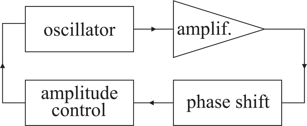
Figure 1: Feedback circuit with signal conditioning for the self–sustained oscillator. Adapted from Ref. 10.

In this paper we study the dynamics of a self–sustained mechanical oscillator driven by elastic and cubic nonlinear forces, i.e. governed by the Duffing equation Nayfeh . It has since long been known that the Duffing equation describes the vibrations of a solid elastic beam clamped at its two ends Narashima ; Tufillaro . More recently, it has been experimentally demonstrated that the motion of a microoscillator consisting of a clamped–clamped silica beam is well–described by the same equation, at least, for small to moderately large oscillation amplitudes NatComm . Our main results are obtained within simplified but realistic approximations, yielding compact and useful analytical expressions. In Sect. 2, we find the frequency and the amplitude of autonomous oscillations in the case where the phase shift introduced by signal conditioning maximizes the oscillator’s response to self–sustaining. In particular, we show that, for hardening and softening nonlinearities, the oscillation frequency respectively increases and decreases as the conditioned amplitude grows. In the latter situation, oscillations are not possible above a certain critical value of that amplitude. In Sect. 3, we move to analyze synchronization of the self–sustained Duffing oscillator under the action of an external harmonic force. There, we obtain our most interesting result: under appropriate conditions, synchronization can be enhanced by making the amplitude of oscillations larger —a counterintuitive effect of nonlinearity. The stability of synchronized motion is assessed numerically. Finally, we draw our conclusions in the last section.

2 The self–sustained Duffing oscillator

The motion of a clamped–clamped micromechanical oscillator in its main oscillation mode is well–described by the Newton equation for a coordinate $x(t)$ quantifying the oscillator’s displacement from equilibrium NatComm :

$$m\ddot{x}+\gamma\dot{x}+kx+k_{3}x^{3}=F_{0}\cos(\phi+\phi_{0})+F_{s}\cos\Omega_{s}t.$$ (1)

Here, $m$, $\gamma$, $k$, and $k_{3}$ are, respectively, the effective mass, damping coefficient, elastic constant and cubic–force coefficient associated to the dynamics of $x$. Positive and negative values of $k_{3}$ correspond, respectively, to hardening and softening cubic forces. The first term in the right–hand side represents the self–sustaining force. Its amplitude $F_{0}$ is fixed by conditioning of the oscillator’s signal, as explained in the Introduction. The angle $\phi$ is the phase associated to the coordinate during oscillatory motion, $x=A\cos\phi$, and $\phi_{0}$ is the phase shift introduced by signal conditioning. The oscillator’s response to the self–sustaining force is maximal for $\phi_{0}=\pi/2$ NatComm ; SADZ , when the force is in–phase with the coordinate’s velocity $\dot{x}$. Additionally, we have included an external harmonic force of amplitude $F_{s}$ and frequency $\phi_{s}$, whose capability of entraining the oscillator into synchronized motion is studied in Sect. 3.

Redefining time as a dimensionless variable, $t\sqrt{k/m}\to t$, Eq. (1) can be rewritten as

$$\ddot{x}+Q^{-1}\dot{x}+x+\beta x^{3}=f_{0}\cos(\phi+\phi_{0})+f_{s}\cos\Omega_{s}t,$$ (2)

with $Q=\sqrt{km}/\gamma$, $\beta=k_{3}/k$, $f_{0}=F_{0}/k$, and $f_{s}=F_{s}/k$. Frequencies are now measured in units of $\omega_{0}=\sqrt{k/m}$, the natural frequency of the corresponding autonomous undamped linear oscillator. Meanwhile, $f_{0}$ and $f_{s}$ have the same units as the coordinate $x$, and $\beta$ has units of $x^{-2}$. Note that the dimensionless quantity $Q$ is the oscillator’s quality factor, which measures the ratio between the decay time due to damping and the oscillation period. Its inverse $Q^{-1}$ gives the ratio between the width of the resonance peak and the resonance frequency.

We first consider Eq. (2) for the unforced self–sustained Duffing oscillator ($f_{s}=0$). In this situation, we expect that —due to the action of the self–sustaining mechanism— the system asymptotically attains periodic oscillations whose amplitude and frequency are determined by its own dynamics. Also, for convenience in the analytical treatment, we fix the phase shift at the value of maximal response: $\phi_{0}=\pi/2$.

An approximate harmonic solution to Eq. (2) can be found by applying the standard procedure of neglecting higher–harmonic terms in the cubic force Landau which, in our case, amount to approximating $\cos^{3}\phi\approx\frac{3}{4}\cos\phi$. In the absence of external forcing, we propose $x(t)=A_{0}\cos\phi\equiv A_{0}\cos\Omega_{0}t$, and separate terms proportional to $\cos\Omega_{0}t$ and $\sin\Omega_{0}t$ to get algebraic equations for the oscillation frequency and amplitude. As shown in the next section, it is convenient to combine these equations into a single equation in the complex domain, which reads

$$(1-\Omega_{0}^{2})A_{0}+\frac{3}{4}\beta A_{0}^{3}+i\left(f_{0}-\frac{\Omega_{0}A_{0}}{Q}\right)=0.$$ (3)

Its solutions are

$$\Omega_{0}=\left(\frac{1+\sqrt{1+3Q^{2}\beta f_{0}^{2}}}{2}\right)^{1/2},\ \ \ \ \ A_{0}=\frac{Qf_{0}}{\Omega_{0}}.$$ (4)

Both $\Omega_{0}$ and the product $|\beta|^{1/2}A_{0}$ depend on the oscillator parameters thorough the combination $\eta=Q|\beta|^{1/2}f_{0}$ only. Note that $\eta\sim 1$ when the oscillation amplitude is such that the nonlinear force becomes comparable to the elastic force, $|\beta|A_{0}^{3}\sim A_{0}$. It is for those values of $\eta$ that the frequency begins to appreciably differ from that of the linear oscillator ($\omega_{0}\equiv 1$). Note also that, for $\beta<0$ and $1+3Q^{2}\beta f_{0}^{2}>0$, an extra solution for the frequency exists: $\Omega_{0}=\left[\frac{1}{2}\left(1-\sqrt{1+3Q^{2}\beta f_{0}^{2}}\right)\right]^{1/2}$. This solution, however, is the analytical continuation for $\beta\neq 0$ of a solution with $\Omega_{0}=0$ and $A_{0}\to\infty$, and is therefore not expected to correspond to stable motion.

Figure 2: The rescaled oscillation amplitude $|\beta|^{1/2}A_{0}$ and the frequency $\Omega_{0}$ as functions of $\eta=Q|\beta|^{1/2}f_{0}$, for both positive and negative $\beta$. The critical value of $\eta$, above which the harmonic solution does not exist for $\beta<0$, is $\eta_{c}=3^{-1/2}$.

Figure 2 shows the rescaled amplitude $|\beta|^{1/2}A_{0}$ and the frequency $\Omega_{0}$ as functions of $\eta$. As could be expected Landau , both for positive and negative $\beta$, the oscillation amplitude grows when the self–sustaining force and/or the quality factor increase. For $\beta>0$, however, the amplitude growth is sublinear, while it is faster than linear for $\beta<0$. Respectively, the oscillation frequency increases and decreases as the amplitude becomes larger.

For $\beta<0$, moreover, the approximate harmonic solution exists for $\eta\leq\eta_{c}=3^{-1/2}\approx 0.577$ only. Above this critical value, the frequency becomes complex, and the solution for $x(t)$ is no more bounded. The effect of nonlinear softening is too strong for the system to sustain oscillations of finite amplitude, and the coordinate grows exponentially.

The stability of the harmonic solution given by Eqs. (4) can be assessed along the same lines as for the ordinary forced Duffing oscillator Nayfeh , namely, assuming that damping, nonlinearities and the external force are perturbations on the harmonic motion of the free linear oscillator. The perturbative calculation, which will be presented elsewhere fase , shows that the harmonic solution for the self–sustained Duffing oscillator is globally stable —i.e., it asymptotically attracts any initial condition— whenever it exists. Even more, this result holds whatever the value of the phase shift $\phi_{0}$ in the self–sustaining force.

3 Synchronized response to harmonic forcing

For the forced self–sustained Duffing oscillator, described by Eq. (2) with $f_{s}\neq 0$, we seek synchronized solutions where the coordinate $x(t)$ oscillates with the same frequency as the external force. Namely, we propose $x(t)=A\cos\phi\equiv A\cos(\Omega_{s}t-\phi_{s})$, where $\phi_{s}$ is the (retarded) phase shift of the coordinate with respect to the force. Replacement in Eq. (2) —always fixing $\phi_{0}=\pi/2$, and within the harmonic approximation for the cubic term— yields algebraic equations for the amplitude $A$ and the phase shift $\phi_{s}$. Combining them into a single equation in the complex domain, we get

$$(1-\Omega_{s}^{2})A+\frac{3}{4}\beta A^{3}+i\left(f_{0}-\frac{\Omega_{s}A}{Q}\right)=f_{s}\exp(-i\phi_{s}),$$ (5)

cf. Eq. (3). Under rather general conditions, solutions to Eq. (5) exist if the synchronization frequency $\Omega_{s}$ lies inside a finite interval which, as we show below, also contains the frequency $\Omega_{0}$ of the unforced oscillator. This interval is the synchronization range Pik ; Manrubia .

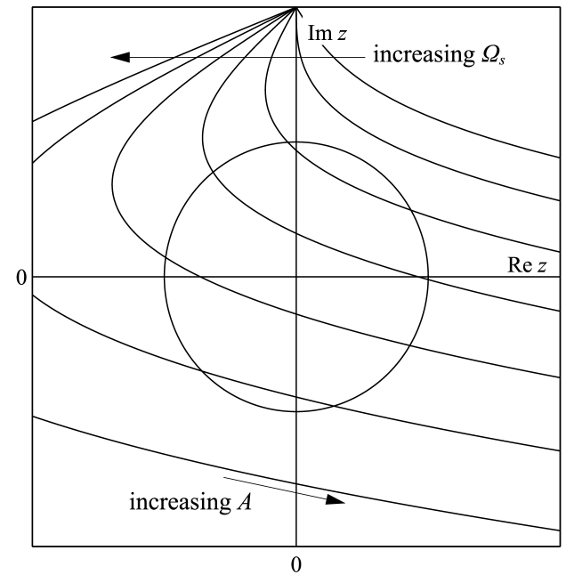
Figure 3: Representation of Eq. (5) on the complex plane $z$. The circle centered at the origin represents the right–hand side of the equation as parametrized by $\phi_{s}$. Its radius is $f_{s}$. The curves represent the left–hand side as parametrized by $A$, for fixed $\beta$ and $Q$, and several values of $\Omega_{s}$. The point on the imaginary axis at which all these curves intersect each other ($A=0$), is $if_{0}$. Along each one of the curves, $A$ increases as indicated by the arrow.

Figure 3 illustrates the situation on the complex plane. The circle centered at the origin, whose radius is $f_{s}$, represents the right–hand side of Eq. (5) as parametrized by the phase shift $\phi_{s}$. The curves represent the left–hand side as parametrized by the amplitude $A$ (with $A\geq 0$), for fixed values of $\beta$ and $Q$, and several values of the frequency $\Omega_{s}$. All these curves pass through the complex number $if_{0}$, on the imaginary axis, for $A=0$. Their curvature is controlled by the nonlinear coefficient $\beta$, while $\Omega_{s}$ determines the slope at $if_{0}$. As $\Omega_{s}$ grows, the curve representing the left–hand side of Eq. (5) “rotates” around $if_{0}$ and, within a finite interval $\Omega_{\min}<\Omega_{s}<\Omega_{\max}$, it intersects the circle at two points. Their polar coordinates give two solutions for $A$ and $\phi_{s}$. For $\Omega_{s}=\Omega_{\min}$ or $\Omega_{\max}$ the curve is tangent to the circle, and the two solutions collapse into a single point.

Note moreover that, by virtue of Eq. (3), the curve representing the left–hand side of Eq. (5) passes through the origin of the complex plane for $\Omega_{s}=\Omega_{0}$ and $A=A_{0}$, given by Eqs. (4). Since, in this situation, the curve necessarily intersects the circle, we conclude that $\Omega_{0}$ lies within the synchronization range $(\Omega_{\min},\Omega_{\max})$.

This latter remark suggests that a way to treat Eq. (5) analytically is to assume that $\Omega_{s}$ and $A$ respectively differ from $\Omega_{0}$ and $A_{0}$ by perturbatively small quantities. The limit is achieved for $f_{s}\to 0$, so that we take as a perturbative parameter the ratio $p=f_{s}/f_{0}$. In the graphical representation of Fig. 3, this amounts to taking the circle’s radius much smaller than the distance to the point of intersection of all the curves on the imaginary axis. Thus, in the vicinity of the circle, the curves can be conveniently approximated by straight segments. To implement the approximation, we write

$$\Omega_{s}=\Omega_{0}+p\delta\Omega,\ \ \ \ \ A=A_{0}+p\delta A.$$ (6)

Expanding Eq. (5) to the first order in $p$ yields

$$z_{0}\delta A-z_{1}\delta\Omega=\exp(-i\phi_{s}),$$ (7)

with

$$z_{0}=\frac{3Q\beta A_{0}}{2\Omega_{0}}-\frac{i}{A_{0}},\ \ \ \ \ z_{1}=2Q+\frac{i}{\Omega_{0}}$$ (8)

Unknowns in Eq. (7) are $\delta A$ and $\phi_{s}$, while $\delta\Omega$ is given in terms of the parameters of our problem through the first of Eqs. (6). A representation of Eq. (7) on the complex plane, similar to that of Fig. 3, makes it immediately possible to show that its solutions exist when $\delta\Omega$ lies in the interval $(-\delta\Omega_{c},\delta\Omega_{c})$, with

$$\delta\Omega_{c}=\frac{1}{|z_{1}||\sin(\zeta_{1}-\zeta_{0})|}.$$ (9)

Here, $\zeta_{k}$ ($k=0,1$) is the argument of the complex number $z_{k}\equiv|z_{k}|\exp(i\zeta_{k})$.

For the sake of concreteness, let us analyze this result in the realistic situation where the oscillator’s quality factor is large, $Q\gg 1$ NatComm . Since —even when the effects of the nonlinear force become sizable— the frequency $\Omega_{0}$ of the unforced self–sustained oscillator is expected to remain of order unity, we can neglect the imaginary part of the complex number $z_{1}$ by comparison to its real part, so that $|z_{1}|=2Q$ and $\zeta_{1}=0$. In this situation, we find

$$\delta\Omega_{c}=\frac{1}{2Q|\sin\zeta_{0}|}=\frac{1}{2Q}\left[\left(\frac{3Q\beta A_{0}^{2}}{2\Omega_{0}}\right)^{2}+1\right]^{1/2}.$$ (10)

Note that, interestingly, this result is independent of the sign of $\beta$: the domain of existence of synchronized solutions does not depend on whether nonlinearities are hardening of softening.

3.1 Analysis of the synchronization range

The half–width of the synchronization range, given by the product $p\delta\Omega_{c}$ [cf. the first of Eqs. (6)], depends on the parameters through the combinations $|\beta|^{1/2}f_{0}$, $|\beta|^{1/2}f_{s}$, and $Q$ only. The dependence on the two latter is simple: $p\delta\Omega_{c}$ is proportional to $|\beta|^{1/2}f_{s}$, and grows monotonically as $Q$ increases with all the other parameters fixed. As expected, the synchronization range widens when the external force and/or the oscillator’s quality factor become larger.

On the other hand, the dependence of the synchronization range on the self–sustaining force is less trivial. When $f_{0}$ grows, the amplitude $A_{0}$ of the self–sustained oscillations increases and, consequently, we expect that the oscillator becomes more difficult to entrain by an external harmonic force of a given amplitude. This is in fact the standard behaviour of a large class of forced oscillating systems, including linear oscillators Pik ; Manrubia ; Nayfeh . For the self–sustained Duffing oscillator, instead, $p\delta\Omega_{c}$ exhibits nonmonotonic behaviour as a function of $|\beta|^{1/2}f_{0}$. This is shown in Fig. 4 for several values of $Q$ and $|\beta|^{1/2}f_{s}=10^{-4}$.

Figure 4: The half–width of the synchronization range, $p\delta\Omega_{c}$, as a function of the rescaled self–sustaining force $|\beta|^{1/2}f_{0}$, for $|\beta|^{1/2}f_{s}=10^{-4}$ and several values of the quality factor $Q$. Dotted labeled straight segments show the slopes in the three regimes. Full dots stand for numerical measurements of the synchronization range for $Q=100$. The dotted curve joining the dots is a spline interpolation plotted as a guide to the eye.

The dependence of $p\delta\Omega_{c}$ on $|\beta|^{1/2}f_{0}$ displays three distinct regimes. For sufficiently small self–sustaining force, the oscillator operates in the linear domain. The oscillation amplitude $A_{0}$ is also small and the frequency is close to the natural value, $\Omega_{0}\approx 1$, such that $Q|\beta|A_{0}^{2}\ll\Omega_{0}$. This inequality can be rewritten as $|\beta|A_{0}^{3}\ll Q^{-1}\Omega_{0}A_{0}$ which, in the equation of motion (2), amounts to having the nonlinear force $\beta x^{3}$ much smaller than the damping force $Q^{-1}\dot{x}$. In this limit, the half–width of the synchronization range reduces to $p\delta\Omega_{c}\approx f_{s}/2Qf_{0}$, and thus decreases with the amplitude of the self–sustaining force as $f_{0}^{-1}$.

The second regime is entered when the nonlinear force overcomes damping, but is still much smaller than the elastic force: $|\beta|A_{0}^{3}\ll A_{0}$. In this situation, the oscillation frequency remains close to unity, but $\delta\Omega_{c}$ is now dominated by the first term inside the square bracket of Eq. (10). The half–width of the synchronization range is $p\delta\Omega_{c}\approx\frac{3}{4}Q^{2}|\beta|f_{s}f_{0}$. Counterintuitively, the synchronization range widens as $f_{0}$ —and, consequently, the oscillation amplitude— grow.

When, finally, the nonlinear force dominates over both damping and the elastic force, the variation of $\Omega_{0}$ with the amplitude cannot be disregarded anymore. We find that, in this limit of large self–sustaining force, $p\delta\Omega_{c}\approx\left(\frac{3}{4}Q^{2}|\beta|\right)^{1/4}f_{s}f_{0}^{-1/2}$. Again, as in the first regime, the half–width of the synchronization range decreases as $f_{0}$ grows, now as $f_{0}^{-1/2}$. The dashed segments in the log–log plot of Fig. 4 show the slopes corresponding to the dependence of $p\delta\Omega_{c}$ on $|\beta|^{1/2}f_{0}$ in the three regimes.

We remark that the boundaries of the three regimes are completely determined by the comparison between the rescaled self–sustaining force $|\beta|^{1/2}f_{0}$ and a suitable power of the quality factor $Q$. Namely, the first transition —from the linear domain to the intermediate regime— occurs for $|\beta|^{1/2}f_{0}\approx Q^{-3/2}$, while the second transition takes place for $|\beta|^{1/2}f_{0}\approx Q^{-1}$. Consequently, as clearly seen in Fig. 4, the three regimes become better separated from each other as $Q$ grows. Note also that, irrespectively of the value of any other parameter, the oscillator is always in the linear regime for $\beta=0$.

Taking into account that the above results have been obtained in the frame of several approximations, it is worthwhile to check their validity by an independent means. With this aim, we have solved Eq. (2) numerically, to determine within which parameter ranges are the synchronized solutions actually observed. The numerical method used to deal with this kind of equation has been discussed elsewhere SADZ . The dots in Fig. 4 stand for the numerical results for the half–width of the synchronization range for $Q=100$. We find very good agreement with the analytical prediction in the linear regime and in most of the intermediate regime, while a noticeable departure is apparent in the upper part of the intermediate regime and for large self-sustaining forces. This discrepancy may be attributed to at least two sources. First, the main approximation involved in the analytical results —namely, the replacement of the cubic term by a single harmonic function— is in fact expected to become increasingly inaccurate as the oscillation amplitude grows. Second, it must be taken into account that numerical and analytical calculations yield, respectively, the ranges of stability and existence of synchronized motion, which are not necessarily coincident SADZ . While we expect that one of the synchronized solutions is stable within its whole existence range, we cannot discard that its observability is jeopardized by the proximity of an unstable solution (see next section), which would lead the system to converge to unsynchronized motion from most initial conditions. Let us emphasize that, in any case, our numerical results confirm the nontrivial behaviour of the synchronization range and, in particular, the presence of an intermediate regime of synchronization enhancement, where the synchronization range widens as the amplitude of oscillations grows.

3.2 Amplitude and phase shift of synchronized motion

To complete the characterization of motion within the synchronization range, we now turn the attention to the amplitude and phase shift of synchronized oscillations. As discussed in connection to Eq. (5), two synchronized solutions exist inside the synchronization range. The fact that, upon variation of the frequency $\Omega_{s}$ of the external forcing, the two solutions appear at $\Omega_{\min}$ and disappear at $\Omega_{\max}$ through tangent (i.e., saddle–node) bifurcations, indicates that one of them is stable and the other unstable.

Within the approximations considered in the previous section, squaring Eq. (7) establishes a quadratic relation between $\delta A$ and $\delta\Omega$, which can be worked out explicitly. Once $\delta A$ has been obtained, it is reinserted in the equation to calculate the phase shift $\phi_{s}$. Note that, in contrast with the half–width of the synchronization range $p\Omega_{c}$, these results are not independent of the sign of the cubic coefficient $\beta$. The upper panels of Fig. 5 show the rescaled amplitude variation, $|\beta|^{1/2}p\delta A$ as a function of the detuning $p\delta\Omega=\Omega_{s}-\Omega_{0}$ for $|\beta|^{1/2}f_{s}=10^{-4}$, $Q=100$, and two values of $|\beta|^{1/2}f_{0}$ in the linear regime and in the intermediate regime (cf. Fig. 4). In both cases, $\beta>0$. The lower panels show the corresponding phase shifts. Full and dashed lines stand for the stable and unstable solutions, respectively. They exist within the synchronization range only, whose boundaries are indicated by the vertical dotted segments.

Figure 5: The rescaled amplitude variation $|\beta|^{1/2}p\delta A$ (upper panels) and the phase shift $\phi_{s}$ (lower panels) of synchronized motion, as functions of the frequency detuning $p\delta\Omega$, for $|\beta|^{1/2}f_{s}=10^{-4}$, $Q=100$, and two self–sustaining force amplitudes: $|\beta|^{1/2}f_{0}=3\times 10^{-4}$ (left) and $3\times 10^{-3}$ (right). Full and dashed curves correspond, respectively, to stable and unstable solutions. The vertical dotted segments indicate the boundaries of the synchronization range $(-p\delta\Omega_{c},p\delta\Omega_{c})$.

For $|\beta|^{1/2}f_{0}=3\times 10^{-4}$, the amplitude of the stable solution first grows with the detuning from a small value at $-p\delta\Omega_{c}$, to a maximum just to the right of $p\delta\Omega=0$. At that point, the oscillator’s response to the external force is maximal. The phase shift is exactly $\phi_{s}=\pi/2$, so that the oscillation velocity and the external force are mutually in–phase. Moreover, they are also in–phase with the self–sustaining signal. As the detuning grows further, the amplitude decreases until the solutions disappear at $p\Omega_{c}$. For $\beta<0$, the behaviour is symmetric with respect to $p\delta\Omega=0$. Namely, the maximal amplitude, with $\phi_{s}=\pi/2$, is reached to the left of exact tuning.

As $|\beta|^{1/2}f_{0}$ becomes larger, the ellipse that represents $|\beta|^{1/2}p\delta A$ as a function of $p\delta\Omega$ narrows toward a straight segment diagonal to the graph. For $|\beta|^{1/2}f_{0}=3\times 10^{-3}$, in the middle of the intermediate regime, the upper–right panel of Fig. 5 shows that the maximal amplitude of the stable solution has strongly shifted to the right, to practically coincide with the upper boundary of the synchronization range. The phase shift has been modified accordingly so that we still have $\phi_{s}=\pi/2$ at the maximum. This trend persists for larger amplitudes of the self–sustaining force: in the limit, the amplitudes of the two solutions lie over the graph’s diagonal while, as the detuning grows within the synchronization range, the phase shift increases from $-\pi/2$ to $\pi/2$ for the stable solution and decreases from $3\pi/2$ ($\equiv-\pi/2$) to $\pi/2$ for the unstable solution.

Whereas, as stated above, $\delta A$ and $\phi_{s}$ can be analytically calculated as functions of $\delta\Omega$, the explicit expressions are too space–consuming to be reported here. We are however able to provide compact expressions in the linear limit, $|\beta|^{1/2}f_{0}\ll Q^{-3/2}$, and for asymptotically large self–sustaining force $|\beta|^{1/2}f_{0}\gg Q^{-1}$ (see Sect. 3.1). In the former case, we have

$$\delta A=\pm 2Q^{2}f_{0}\sqrt{1-\left(\frac{\delta\Omega}{2Q}\right)^{2}},\ \ \ \ \ \exp(i\phi_{s})=-2Q\delta\Omega\pm i\sqrt{1-4Q^{2}\delta\Omega^{2}},$$ (11)

where the upper and lower signs correspond, respectively, to the stable and unstable solutions. Meanwhile, the large–$f_{0}$ limit yields

$$\delta A=\frac{2\delta\Omega}{\sqrt{3|\beta|}}\mbox{ for $|\delta\Omega|<\delta\Omega_{c}$},\ \ \ \ \ \exp(i\phi_{s})=\pm\sqrt{1-\left(\frac{\delta\Omega}{\delta\Omega_{c}}\right)^{2}}+i\frac{\delta\Omega}{\delta\Omega_{c}},$$ (12)

with $\delta\Omega_{c}$ as given in Sect. 3.1 for the same limit.

4 Conclusion

In this paper, we have characterized the autonomous dynamics and the synchronizability by a harmonic external force of a self–sustained Duffing oscillator. The self–sustaining mechanism allows the system to maintain oscillatory motion with internally defined amplitude and frequency. As expected, the frequency increases or decreases as the amplitude grows, respectively, for hardening and softening nonlinearities. Synchronization with the external force is possible when the detuning between the force’s and the oscillator’s frequency lies below a certain critical value. Our analysis holds for a specific phase shift in the self–sustaining mechanism, corresponding to the expected maximum in the oscillator’s resonant response to the feedback signal. Due to unavoidable experimental fluctuations in that value, however, it would be worthwhile devoting future work to relax such condition.

Our most relevant result regards the existence of a regime of synchronization enhancement where the synchronization range widens as the amplitude of oscillations becomes larger —a counterintuitive effect of nonlinearities, found for intermediate amplitudes of the self–sustaining force. Interestingly enough, this regime has already been observed in experiments with micromechanical oscillators consisting of clamped–clamped silica bars DD , although results have not been published yet. Moreover, this seems to be the most natural operation regime of this kind of micromechanical oscillators with lengths of the order of hundreds of microns, and quality factors around $10^{4}$ NatComm . For self–sustaining amplitudes in the linear regime, in fact, the oscillation amplitudes are too small to provide a signal discernible from electronic noise. For large amplitudes, on the other hand, results suggest that the oscillator abandons the parameter region where it is well described by the Duffing model, and a different description may prove necessary. A sudden increase in the size of the synchronization range, that could be related to the phenomenon described here, has also been recently reported for mutually coupled oscillators Agr .

It remains to be explored whether the regime of synchronization enhancement might be advantageously exploited in applications where, beyond individually producing a sustained periodic signal, two or more micromechanical oscillators are expected to synchronize to each other. This would be the case in building up a more robust periodic signal —able to overcome the effects of electronic and/or thermal noise— or in devices where synchronous coherent motion of many oscillators is required, such as in optical components for communication systems CH ; Ek . The collective dynamics of an ensemble of coupled self–sustained Duffing oscillators is per se an attractive problem that deserves future consideration.

References

- (1) S. Strogatz, Sync: The Emerging Science of Spontaneous Order (Hyperion, New York, 2003)
- (2) A. Pikovsky, M. Rosenblum, J. Kuths, Synchronization: A Universal Concept in Nonlinear Sciences (Cambridge University Press, Cambridge, 2003)
- (3) S. C. Manrubia, A. S. Mikhailov, D. H. Zanette, Emergence of Dynamical Order. Synchronization Phenomena in Complex Systems (World Scientific, Singapore, 2004)
- (4) Y. Kuramoto, Chemical Oscillations, Waves, and Turbulence (Springer, Berlin, 1984)
- (5) A. T. Winfree, The Geometry of Biological Time (Springer, New York, 2001)
- (6) H. F. El–Nashar, H. A. Cerdeira, Chaos 19, 033127 (2009)
- (7) P. F. C. Tilles, F. F. Ferreira, H. A. Cerdeira, Phys. Rev. E 83, 066206 (2011)
- (8) H. G. Craighead, Science 290, 1532 (2000)
- (9) K. L. Ekinci and M. L. Roukes, Rev. Sci. Instrum. 76, 061101 (2005)
- (10) B. Yurke, D. S. Greywall, A. N. Pargellis, P. A. Busch, Phys. Rev. A 51, 4211 (1995)
- (11) A. H. Nayfeh, D. T. Mook, Nonlinear Oscillations (Wiley, New York, 1995)
- (12) R. Narashima, J. Sound Vib. 8, 464 (1968)
- (13) T. C. Molteno, N. B. Tufillaro, Am. J. Phys. 72, 1157 (2004)
- (14) D. Antonio, D. H. Zanette, D. López, Nat. Commun. 3, 802 (2012)
- (15) S. I. Arroyo, D. H. Zanette, Phys. Rev. E 87, 052910 (2013)
- (16) L. Landau, E. Lifshitz, Mechanics. Course on Theoretical Physics, Vol. 1 (Butterworth–Heinemann, Oxford, 1976)
- (17) S. I. Arroyo, D. H. Zanette, in preparation
- (18) D. Antonio, D. López, J. Guest, D. Czaplewski, private communication
- (19) D. K. Agrawal, J. Woodhouse, A. A. Seshia, Phys. Rev. Lett. 111, 084101 (2013)