Finite temperature fermionic charge and current densities
induced by a cosmic string with magnetic flux

Abstract

We investigate the finite temperature expectation values of the charge and current densities for a massive fermionic field with nonzero chemical potential, $\mu$, in the geometry of a straight cosmic string with a magnetic flux running along its axis. These densities are decomposed into the vacuum expectation values and contributions coming from the particles and antiparticles. The charge density is an even periodic function of the magnetic flux with the period equal to the quantum flux and an odd function of the chemical potential. The only nonzero component of the current density corresponds to the azimuthal current. The latter is an odd periodic function of the magnetic flux and an even function of the chemical potential. At high temperatures, the parts in the charge density and azimuthal current induced by the planar angle deficit and magnetic flux are exponentially small. The asymptotic behavior at low temperatures crucially depends whether the value $|\mu|$ is larger or smaller than the mass of the field quanta, $m$. For $|\mu|<m$ the charge density and the contributions into the azimuthal current coming from the particles and antiparticles are exponentially suppressed at low temperatures. In the case $|\mu|>m$, the charge and current densities receive two contributions coming from the vacuum expectation values and from particles or antiparticles (depending on the sign of chemical potential). At large distances from the string the latter exhibits a damping oscillatory behavior with the amplitude inversely proportional to the square of the distance.

PACS numbers: 03.70.+k, 11.10.Wx, 11.27.+d, 98.80.Cq

1 Introduction

In 1973, Nielsen and Olesen proposed a theoretical model comprised by Higgs and gauge fields, that produces linear topological defect carrying a magnetic flux named ‘vortex’ [1]. A few years later, Garfinkle investigated the influence of the vortex on the geometry of the spacetime [2]. Coupling the energy-momentum tensor associated with the system to the Einstein equations, he found static cylindrically symmetric solutions. The author also showed that, asymptotically, the spacetime around the vortex is a Minkowski one minus a wedge. The core of the vortex has a nonzero thickness and a magnetic flux through it. Two years later, Linet [3] obtained exact solutions for the complete set of differential equations, for some specific conditions. The author showed that the structure of the respective spacetime corresponds to a conical one, with the conicity parameter being expressed in terms of the energy per unit length of the vortex.

The cosmic strings are among the most important class of linear topological defects with the conical geometry outside the core [4]. The formation of this type of topologically stable structures during the cosmological expansion is predicted in most interesting models of high energy physics. They have a number of interesting observable consequences, the detection of which would provide an important link between cosmology and particle physics. In the eighties of last century, the interest to cosmic strings was mainly due to the fact that they provide a mechanism for the large-scale structure formation in the universe which is alternative to the one based on inflationary paradigm. Though the recent observations of the cosmic microwave background radiation have ruled out the scenario in which the cosmic strings seed the primordial density perturbations, they are sources of a number of interesting effects which include the generation of gravitational waves, high energy cosmic rays, and gamma ray bursts. Among the other signatures of the cosmic strings, we mention here the gravitational lensing, the creation of small non-Gaussianities in the cosmic microwave background and the influence on the corresponding tensor-modes. The recent progress in models with large compact dimensions and large warp factors have shown that the fundamental strings can act as cosmic strings. In particular, a new formation mechanism for cosmic strings is proposed in the framework of brane inflation [5]. The cosmic string type conical defects appear also in condensed matter systems such as crystals, liquid crystals and quantum liquids (see, for example, Ref. [6]).

In quantum field theory, the nontrivial spatial topology due to the presence of a cosmic string causes a number of interesting physical effects. In particular, many authors have considered the vacuum polarization for scalar, fermionic and vector fields induced by a planar angle deficit. Among the main local characteristics of the vacuum state, the expectation values of the field squared and of the energy-momentum tensor have been investigated. In addition to the deficit angle parameter, the physical origin of a cosmic string is characterized by the gauge field flux parameter describing a magnetic flux running along the string core. The latter induces additional polarization effects for charged fields [7]-[12]. Though the gauge field strength vanishes outside the string core, the nonvanishing vector potential leads to Aharonov-Bohm-like effects on scattering cross sections and on particle production rates around the cosmic string [13].

For charged fields, the magnetic flux along the string core induces nonzero vacuum expectation value of the current density. The latter, in addition to the expectation values of the field squared and the energy-momentum tensor, is among the most important local characteristics of the vacuum state for quantum fields. The expectation value of the current density acts as a source in semiclassical Maxwell equations and plays a crucial role in modeling a self-consistent dynamics involving the electromagnetic field. The azimuthal current density for scalar and fermionic fields, induced by a magnetic flux in the geometry of a straight cosmic string, has been investgated in [14]-[18]. The fermionic current induced by a magnetic flux in a $(2+1)$-dimensional conical spacetime with a circular boundary has been analyzed in [19]. The compactification of the cosmic string along its axis may lead to the appearance of the axial current density [17, 18] (for the vacuum expectation value of the current density in models with compact dimensions see [20] in the case of flat background geometry and [21, 22] for de Sitter and anti-de Sitter bulks). The generalization of the corresponding results for the fermionic case to a cosmic string in the background of de Sitter spacetime is given in [23]. All these considerations of the current density around a cosmic string deal with the idealized geometry where the string is assumed to have zero thickness. Realistic cosmic strings have internal structure, characterized by the core radius determined by the symmetry breaking scale at which it is formed. The vacuum expectation value of the current density for a massive charged scalar field in the geometry of a cosmic string with a general cylindrically symmetric core of a finite support is investigated in [24]. In the corresponding model, the core encloses a gauge field flux directed along the string axis with an arbitrary radial distribution.

Continuing in this line of investigations, in the present paper we consider the effects of the finite temperature and nonzero chemical potential on the expectation values of the charge and current densities for a massive fermionic field in the geometry of a straight cosmic string for arbitrary values of the planar angle deficit (for combined effects of the finite temperature and nontrivial spatial topology on the expectation values of the charge and current densities for scalar and fermionic fields in models with toroidally compactified dimensions see [25, 26]). This is an important topic, since for a cosmic string in the early stages of the cosmological expansion the typical state of a quantum field is a state containing particles in thermal equilibrium. The finite temperature expectation value of the energy density for a massless scalar field around a cosmic string in the absence of the magnetic flux is derived in [27] for integer values of the parameter $q=2\pi/\phi_{0}$, where $2\pi-\phi_{0}$ is the planar angle deficit. The expectation value of a renormalized energy-momentum tensor for a general case of the parameter $q\geqslant 1$ has been considered in [28] for a conformally coupled massless scalar field and in [29] for a general case of a curvature coupling parameter. Guimarães [30] has extended the corresponding results for a magnetic flux cosmic string assuming that $q<2$. The thermal average of the energy-momentum tensor for massless fermions has been investigated in [31], again, under the assumption $q<2$.

This paper is structured as follows. In the next section we describe the background geometry associated with the spacetime under consideration and construct a complete set of normalized positive- and negative-energy fermionic mode functions. By using these functions, the thermal average of the charge density is investigated in section 3. Various asymptotic limits are considered in detail, including the low- and high-temperature asymptotics. The only nonzero component of the thermal average for the current density corresponds to the azimuthal current. The corresponding expression is derived in section 4. The expectation value is decomposed into the vacuum expectation value and the contributions coming from particles and antiparticles. The behavior of the current density in the asymptotic regions of the parameters is discussed. The main results of the paper are summarized in section 5.

2 Geometry and the fermionic modes

The background geometry corresponding to a straight cosmic string lying along the $z$-axis can be written through the line element

$$ds^{2}=dt^{2}-dr^{2}-r^{2}d\phi^{2}-dz{}^{2}\ ,$$ (2.1)

where $r\geqslant 0$, $0\leqslant\phi\leqslant\phi_{0}=2\pi/q$, $-\infty<t<+\infty$. The parameter $q\geqslant 1$ codifies the planar angle deficit and is related to the linear mass density of the string $\mu_{0}$ as $q^{-1}=1-4\mu_{0}$. In the presence of an external electromagnetic field with the vector potential $A_{\mu}$, the dynamics of a massive charged spinor field in curved spacetime is described by the Dirac equation,

$$(i\gamma^{\mu}{\mathcal{D}}_{\mu}-m)\psi=0\ ,\ {\mathcal{D}}_{\mu}=\partial_{\mu}+\Gamma_{\mu}+ieA_{\mu},$$ (2.2)

where $\gamma^{\mu}$ are the Dirac matrices in curved spacetime and $\Gamma_{\mu}$ are the spin connections. For the geometry at hand the gamma matrices can be taken in the form (see, for instance, [17])

$$\gamma^{0}=\left(\begin{array}[]{cc}1&0\\ 0&-1\end{array}\right),\;\gamma^{l}=\left(\begin{array}[]{cc}0&\rho^{l}\\ -\rho^{l}&0\end{array}\right),$$ (2.3)

where the $2\times 2$ matrices $\rho^{l}$ are

$$\rho^{1}=\left(\begin{array}[]{cc}0&e^{-iq\phi}\\ e^{iq\phi}&0\end{array}\right)\ ,\ \rho^{2}=-\frac{i}{r}\left(\begin{array}[]{cc}0&e^{-iq\phi}\\ -e^{iq\phi}&0\end{array}\right)\ ,\ \rho^{3}=\left(\begin{array}[]{cc}1&0\\ 0&-1\end{array}\right)\ .$$ (2.4)

The only nonzero component of the spin connection corresponds to $\mu=2$:

$$\Gamma_{\mu}=i\frac{q-1}{2}\left(\begin{array}[]{cc}\rho^{3}&0\\ 0&\rho^{3}\end{array}\right)\delta_{\mu}^{2},$$ (2.5)

and in the Dirac equation one has $\gamma^{\mu}\Gamma_{\mu}=(1-q)\gamma^{1}/(2r)$.

We shall admit the existence of a gauge field with the constant vector potential as

$$A_{\mu}=(0,0,A_{2},0)\ .$$ (2.6)

The azimuthal component $A_{2}$ is related to an infinitesimal thin magnetic flux, $\Phi$, running along the string, as $A_{2}=-q\Phi/(2\pi)$. Although the magnetic field strength corresponding to the vector potential (2.6) vanishes, the magnetic flux along the cosmic string leads to Aharonov-Bohm-like effects on the expectation values of physical observables. In particular, as it will be shown below, it induces a nonzero expectation value of the current density.

Here, we are interested in the effects of the presence of the cosmic string and magnetic flux on the expectation values of the charge and current densities assuming that the field is in thermal equilibrium at finite temperature $T$. We shall use the same procedure as in [26] to evaluate these physical observables at finite temperature. The standard form of the density matrix for the thermodynamical equilibrium distribution at temperature $T$ is

$$\hat{\rho}=Z^{-1}e^{-\beta(\hat{H}-\mu^{\prime}\hat{Q})},\;\beta=1/T,$$ (2.7)

where $\hat{H}$ is the Hamilton operator, $\hat{Q}$ denotes a conserved charge and $\mu^{\prime}$ is the corresponding chemical potential. The grand canonical partition function $Z$ is given by

$$Z=\mathrm{tr}[e^{-\beta(\hat{H}-\mu^{\prime}\hat{Q})}].$$ (2.8)

Let $\{\psi_{\sigma}^{(+)},\psi_{\sigma}^{(-)}\}$ be a complete set of normalized positive- and negative-energy solutions of (2.2), specified by a set of quantum numbers $\sigma$. In order to evaluate the fermionic current densities we expand the field operator as

$$\psi=\sum_{\sigma}[\hat{a}_{\sigma}\psi_{\sigma}^{(+)}+\hat{b}_{\sigma}^{+}\psi_{\sigma}^{(-)}]\ ,$$ (2.9)

where $\hat{a}_{\sigma}$ and $\hat{b}_{\sigma}^{+}$ represent the annihilation and creation operators corresponding to particles and antiparticles respectively, and use the relations

$$\mathrm{tr}[\hat{\rho}\hat{a}_{\sigma}^{+}\hat{a}_{\sigma^{\prime}}] = \frac{\delta_{\sigma\sigma^{\prime}}}{e^{\beta(\varepsilon_{\sigma}^{(+)}-\mu)}+1},$$

$$\mathrm{tr}[\hat{\rho}\hat{b}_{\sigma}^{+}\hat{b}_{\sigma^{\prime}}] = \frac{\delta_{\sigma\sigma^{\prime}}}{e^{\beta(\varepsilon_{\sigma}^{(-)}+\mu)}+1},$$ (2.10)

where $\mu=e\mu^{\prime}$ and $\pm\varepsilon_{\sigma}^{(\pm)}$ with $\varepsilon_{\sigma}^{(\pm)}>0$, are the energies corresponding to the modes $\psi_{\sigma}^{(\pm)}$.

The expectation value of the fermionic current density is given by

$$\left\langle j^{\nu}\right\rangle=e\,\mathrm{tr}[\hat{\rho}\bar{\psi}(x)\gamma^{\nu}\psi(x)].$$ (2.11)

Substituting the expansion (2.9) and using the relations (2.10), the current density is decomposed as

$$\left\langle j^{\nu}\right\rangle=\left\langle j^{\nu}\right\rangle_{0}+\sum_{\chi=+,-}\left\langle j^{\nu}\right\rangle_{\chi},$$ (2.12)

where

$$\left\langle j^{\nu}\right\rangle_{0}=e\sum_{\sigma}\bar{\psi}_{\sigma}^{(-)}(x)\gamma^{\nu}\psi_{\sigma}^{(-)}(x),$$ (2.13)

is the vacuum expectation value and

$$\left\langle j^{\nu}\right\rangle_{\pm}=\pm e\sum_{\sigma}\frac{\bar{\psi}_{\sigma}^{(\pm)}\gamma^{\nu}\psi_{\sigma}^{(\pm)}}{e^{\beta(\varepsilon_{\sigma}^{(\pm)}\mp\mu)}+1}.$$ (2.14)

Here, $\left\langle j^{\nu}\right\rangle_{\pm}$ is the part in the expectation value coming from the particles for the upper sign and from the antiparticles for the lower sign.

As is seen, for the evaluation of the current density we need a complete set of fermionic modes. In Ref. [17], it has been shown that the positive- and negative-energy fermionic mode-functions are uniquely specified by the set of quantum numbers $\sigma=(\lambda,k,j,s)$ with

$$\lambda\geqslant 0,\;-\infty<k<+\infty,\;j=\pm 1/2,\pm 3/2,\ldots,\;s=\pm 1.$$ (2.15)

These functions are expressed as

$$\psi_{\sigma}^{(\pm)}(x)=C_{\sigma}^{(\pm)}e^{\mp iEt+ikz+iqj\phi}\left(\begin{array}[]{c}J_{\beta_{j}}(\lambda r)e^{-iq\phi/2}\\ sJ_{\beta_{j}+\epsilon_{j}}(\lambda r)e^{iq\phi/2}\\ \pm\frac{k-is\epsilon_{j}\lambda}{E\pm m}J_{\beta_{j}}(\lambda r)e^{-iq\phi/2}\\ \mp s\frac{k-is\lambda\epsilon_{j}}{E\pm m}J_{\beta_{j}+\epsilon_{j}}(\lambda r)e^{iq\phi/2}\end{array}\right)\ ,$$ (2.16)

where $J_{\nu}(x)$ is the Bessel function,

$$E=\varepsilon_{\sigma}^{(\pm)}=\sqrt{\lambda^{2}+k^{2}+m^{2}},$$ (2.17)

and

$$\beta_{j}=q|j+\alpha|-\epsilon_{j}/2\ ,\;\alpha=eA_{2}/q=-\Phi/\Phi_{0},$$ (2.18)

with $\epsilon_{j}=\mathrm{sgn}(j+\alpha)$ and $\Phi_{0}=2\pi/e$ being the flux quantum. The wave functions (2.16) are eigenfunctions of the projection of total angular momentum operator along the cosmic string,

$$\hat{J}_{3}\psi_{\sigma}^{(\pm)}=\left(-\frac{i}{q}(\partial_{2}+ieA_{2})+\frac{1}{2}\left(\begin{array}[]{cc}\rho^{3}&0\\ 0&\rho^{3}\end{array}\right)\right)\psi_{\sigma}^{(\pm)}=(j+\alpha)\psi_{\sigma}^{(\pm)},$$ (2.19)

with the eigenvalues $j+\alpha$.

The constants $C_{\sigma}^{(\pm)}$ in (2.16) are determined by the orthonormalization condition

$$\int d^{3}x\sqrt{\gamma}\ (\psi_{\sigma}^{(\pm)})^{\dagger}\psi_{\sigma^{\prime}}^{(\pm)}=\delta_{\sigma\sigma^{\prime}}\ ,$$ (2.20)

where $\gamma$ is the determinant of the spatial metric tensor. The delta symbol on the right-hand side is understood as the Dirac delta function for continuous quantum numbers ($\lambda,k$) and the Kronecker delta for discrete ones ($j,s$). From (2.20) one obtains

$$|C_{\sigma}^{(\pm)}|^{2}=\frac{q\lambda(E\pm m)}{16\pi^{2}E}\ .$$ (2.21)

In defining the fermionic mode functions (2.16) we have imposed the regularity condition at the cone apex. It is well known that for an idealized zero thickness magnetic flux the theory of von Neumann deficiency indices leads to a one-parameter family of boundary conditions [32]. In addition to the regular modes, these conditions, in general, allow normalizable irregular modes. The expectation values of the charge and current densities for general boundary conditions are evaluated in a way similar to that described below. The contribution of the regular modes is the same for all boundary conditions and the expressions differ by the contributions coming from the irregular modes. Note that in a recent investigation of the induced fermionic current for a massless Dirac field in (2+1) dimensions [33], the authors impose the regularity condition. The corresponding result agrees with that for a finite radius solenoid, assuming that fermions cannot penetrate the region of nonzero magnetic flux.

The fermionic charge and current densities at zero temperature, $\left\langle j^{\mu}\right\rangle_{0}$, have been investigated in [17] for zero chemical potential. Therefore, we will be mainly concerned with the contributions from particles and antiparticles provided by the second term in the right-hand side of (2.12).

3 Charge density

We start with the charge density corresponding to the $\nu=0$ component in (2.12). As it has been shown in [17], the vacuum expectation value of the charge density vanishes, $\left\langle j^{0}\right\rangle_{0}=0$. Substituting the mode functions (2.16) into (2.14), for the contributions coming from the particles and antiparticles we get

$$\left\langle j^{0}\right\rangle_{\pm}=\pm\frac{eq}{8\pi^{2}}\sum_{\sigma}\lambda\frac{J_{\beta_{j}}^{2}(\lambda r)+J_{\beta_{j}+\epsilon_{j}}^{2}(\lambda r)}{e^{\beta(E\mp\mu)}+1},$$ (3.1)

where we use the notation

$$\sum_{\sigma}=\int_{-\infty}^{+\infty}dk\int_{0}^{\infty}d\lambda\ \sum_{s=\pm 1}\sum_{j}\ .$$ (3.2)

Here and in what follows

$$\sum_{j}=\sum_{j=\pm 1/2,\pm 3/2,\cdots}.$$ (3.3)

As is seen, in the case $\mu=0$ the contributions from the particles and antiparticles cancel each other and the total charge density,

$$\left\langle j^{0}\right\rangle=\left\langle j^{0}\right\rangle_{+}+\left\langle j^{0}\right\rangle_{-},$$ (3.4)

is zero. For $\mu>0$ ($\mu<0$) the particles (antiparticles) dominate and $\left\langle j^{0}\right\rangle/e>0$ ($\left\langle j^{0}\right\rangle/e<0$). From (3.1) it follows that the charge density is an even periodic function of the parameter $\alpha$ with the period equal to 1. This means that the charge density is a periodic function of the magnetic flux with the period equal to the quantum flux. If we present this parameter as

$$\alpha=n_{0}+\alpha_{0},\;|\alpha_{0}|\leqslant 1/2,$$ (3.5)

with $n_{0}$ being an integer, then the current density depends on $\alpha_{0}$ alone.

For the further transformation of the expression (3.1), first we consider the case $|\mu|<$ $m$. With this assumption, by using the expansion

$$(e^{y}+1)^{-1}=-\sum_{n=1}^{\infty}(-1)^{n}e^{-ny}\ ,$$ (3.6)

after the summation over $s$, we obtain

$$\left\langle j^{0}\right\rangle_{\pm} = \mp\frac{eq}{2\pi^{2}}\sum_{n=1}^{\infty}(-1)^{n}e^{\pm n\beta\mu}\sum_{j}\int_{0}^{\infty}dk$$ (3.7)

$$\times\int_{0}^{\infty}d\lambda\,\lambda[J_{\beta_{j}}^{2}(\lambda r)+J_{\beta_{j}+\epsilon_{j}}^{2}(\lambda r)]e^{-n\beta E}\ .$$

As the next step, we use the integral representation

$$e^{-n\beta E}=\frac{n\beta}{\sqrt{\pi}}\int_{0}^{\infty}ds\,s^{-2}e^{-(\lambda^{2}+k^{2}+m^{2})s^{2}-n^{2}\beta^{2}/4s^{2}},$$ (3.8)

and the relation [34]

$$\int_{0}^{\infty}d\lambda\ \lambda e^{-s^{2}\lambda^{2}}[J_{\beta_{j}}^{2}(\lambda r)+J_{\beta_{j}+\epsilon_{j}}^{2}(\lambda r)]=\frac{e^{-x}}{2s^{2}}\left[I_{\beta_{j}}(x)+I_{\beta_{j}+\epsilon_{j}}(x)\right]\ ,$$ (3.9)

with $x=r^{2}/(2s^{2})$ and $I_{\nu}(x)$ being the modified Bessel function. After integration over $k$, we get

$$\left\langle j^{0}\right\rangle_{\pm} = \mp\frac{eq\beta}{4\pi^{2}r^{4}}\ \sum_{n=1}^{\infty}(-1)^{n}ne^{\pm n\beta\mu}\int_{0}^{\infty}dx\,x$$ (3.10)

$$\times F(q,\alpha_{0},x)e^{-m^{2}r^{2}/2x-(1+n^{2}\beta^{2}/2r^{2})x}\ ,$$

where the notation

$$F(q,\alpha_{0},x)=\sum_{j}\ \left[I_{\beta_{j}}(x)+I_{\beta_{j}+\epsilon_{j}}(x)\right],$$ (3.11)

is introduced

An alternative representation for the charge density is obtained by making use of the integral representation for the series $\sum_{j}I_{\beta_{j}}(x)$ derived in [19]. With this representation, the function (3.11) is expressed as

$$F(q,\alpha_{0},x) = \frac{4}{q}\left[\frac{e^{x}}{2}+\sum_{k=1}^{[q/2]}(-1)^{k}c_{k}\cos\left(2\pi k\alpha_{0}\right)e^{x\cos(2\pi k/q)}\right.$$ (3.12)

$$\left.+\frac{q}{\pi}\int_{0}^{\infty}dy\frac{h(q,\alpha_{0},2y)\sinh y}{\cosh(2qy)-\cos(q\pi)}e^{-x\cosh{(2y)}}\right]\ ,$$

where $[q/2]$ means the integer part of $q/2$ and the notation

$$h(q,\alpha_{0},x)=\sum_{\chi=\pm 1}\cos\left[\left(1/2+\chi\alpha_{0}\right)q\pi\right]\sinh\left[\left(1/2-\chi\alpha_{0}\right)qx\right],$$ (3.13)

is assumed. Here and in what follows we use the notations

$$c_{k}=\cos{(\pi k/q),\;s}_{k}=\sin{(\pi k/q).}$$ (3.14)

Substituting (3.12) into (3.10), after integration over $x$, we find the expression

$$\left\langle j^{0}\right\rangle_{\pm} = \left\langle j^{0}\right\rangle_{\mathrm{M}\pm}\mp\frac{2em^{4}\beta}{\pi^{2}}\ \sum_{n=1}^{\infty}(-1)^{n}ne^{\pm n\beta\mu}$$ (3.15)

$$\times\left[\sum_{k=1}^{[q/2]}(-1)^{k}c_{k}\cos\left(2\pi k\alpha_{0}\right)f_{2}(m\beta s_{n}(r/\beta,k/q))\right.$$

$$\left.+\frac{q}{\pi}\int_{0}^{\infty}dy\frac{\sinh\left(y\right)h(q,\alpha_{0},2y)}{\cosh(2qy)-\cos(q\pi)}f_{2}(m\beta c_{n}(r/\beta,y))\right],$$

where

$$\left\langle j^{0}\right\rangle_{\mathrm{M}\pm}=\mp\frac{e\beta m^{4}}{\pi^{2}}\sum_{n=1}^{\infty}(-1)^{n}ne^{\pm n\beta\mu}f_{2}(nm\beta),$$ (3.16)

is the corresponding charge density in Minkowski spacetime in the absence of the magnetic flux and the cosmic string ($\alpha_{0}=0$, $q=1$). Here we have introduced the notations

$$f_{\nu}(x)=x^{-\nu}K_{\nu}(x),$$ (3.17)

with $K_{\nu}(x)$ being the MacDonald function and

$$s_{n}(x,y) = \sqrt{n^{2}+4x^{2}\sin^{2}(\pi y)},$$

$$c_{n}(x,y) = \sqrt{n^{2}+4x^{2}\cosh^{2}y}\ .$$ (3.18)

For the total charge density one gets

$$\left\langle j^{0}\right\rangle = -\frac{4em^{4}\beta}{\pi^{2}}\ \sum_{n=1}^{\infty}(-1)^{n}n\sinh(n\beta\mu)\left[\frac{1}{2}f_{2}(m\beta n)\right.$$ (3.19)

$$+\sum_{k=1}^{[q/2]}(-1)^{k}c_{k}\cos\left(2\pi k\alpha_{0}\right)f_{2}(m\beta s_{n}(r/\beta,k/q))$$

$$\left.+\frac{q}{\pi}\int_{0}^{\infty}dy\frac{h(q,\alpha_{0},2y)\sinh y}{\cosh(2qy)-\cos(q\pi)}f_{2}(m\beta c_{n}(r/\beta,y))\right],$$

where the contribution coming from the first term in the square brackets corresponds to the charge density in Minkowski spacetime, $\left\langle j^{0}\right\rangle_{\mathrm{M}}=\left\langle j^{0}\right\rangle_{\mathrm{M}+}+\left\langle j^{0}\right\rangle_{\mathrm{M}-}$. Note that the expression (3.19) is also valid in the case $|\mu|=m$. In the absence of the conical defect, $q=1$, the expression (3.19) reduces to

$$\left\langle j^{0}\right\rangle =-\frac{2em^{4}\beta}{\pi^{2}}\sum_{n=1}^{\infty}(-1)^{n}n\sinh(n\beta\mu)\left[f_{2}(nm\beta)\right.$$

$$+\left.\frac{2}{\pi}\sin\left(\alpha_{0}\pi\right)\int_{0}^{\infty}dy\,\tanh y\sinh\left(2\alpha_{0}y\right)f_{2}\left(m\beta c_{n}(r/\beta,y)\right)\right],$$ (3.20)

where the second term in the square brackets is induced by the magnetic flux.

Let us consider the behavior of the charge density in various asymptotic regions of the parameters. First we consider the region near the string. For $2|\alpha_{0}|\leqslant 1-1/q$, the charge density is finite on the string. The corresponding limiting value is directly obtained from (3.19) by taking $r=0$:

$$\left\langle j^{0}\right\rangle_{r=0}=-\frac{2em^{4}\beta}{\pi^{2}}\left[1+2h_{0}(q,\alpha_{0})\right]\sum_{n=1}^{\infty}(-1)^{n}n\sinh(n\beta\mu)f_{2}(nm\beta),$$ (3.21)

where we have used the notation

$$h_{n}(q,\alpha_{0})=\sum_{k=1}^{[q/2]}(-1)^{k}\frac{c_{k}}{s_{k}^{n}}\cos\left(2\pi k\alpha_{0}\right)+\frac{q}{\pi}\int_{0}^{\infty}dy\ \frac{h(q,\alpha_{0},2y)\sinh\left(y\right)\cosh^{-n}y}{\cosh(2qy)-\cos(q\pi)}.$$ (3.22)

In the case $2|\alpha_{0}|>1-1/q$ the charge density diverges on the string. This divergence comes from the integral term in (3.19). In order to find the leading term in the corresponding asymptotic expansion over the distance from the string, we note that for small $r$ the dominant contribution to the integral comes from large values of $y$. By using the corresponding asymptotic, the integral over $y$ is expressed in terms of the MacDonald function and to the leading order one gets

$$\left\langle j^{0}\right\rangle\approx-\frac{eqm^{4}\beta(mr/\sqrt{2})^{\left(1-2|\alpha_{0}|\right)q-1}}{\pi^{2}\Gamma(1/2+\left(1/2-|\alpha_{0}|\right)q)}\sum_{n=1}^{\infty}(-1)^{n}n\sinh(n\beta\mu)f_{3/2+\left(1/2-|\alpha_{0}|\right)q}(nm\beta).$$ (3.23)

As is seen, the divergence is integrable and, hence, the part in the total charge per unit length of the string, induced by the cosmic string and magnetic flux, is finite. We denote this charge by $\Delta Q$. The charge density, induced by the cosmic string and magnetic flux, is given by the second and third terms in the square brackets of (3.19). After integration of this part over the radial and angular coordinates, one gets

$$\Delta Q=-\frac{2em^{2}\beta}{\pi q}h_{2}(q,\alpha_{0})\ \sum_{n=1}^{\infty}(-1)^{n}n\sinh(n\beta\mu)f_{1}(m\beta n).$$ (3.24)

For sufficiently large $r_{0}$, the total charge (per unit length of the string) in the cylindrical volume of the radius $r_{0}$ can be written as

$$Q=\frac{1}{2}\phi_{0}r_{0}^{2}\left\langle j^{0}\right\rangle_{\mathrm{M}}+\Delta Q.$$ (3.25)

Now let us consider the asymptotic behavior of the charge density at low and high temperatures. At low temperatures, $T\ll m,r^{-1}$, and for $|\alpha_{0}|<1/2-1/(2q)$, in the arguments of the functions $f_{2}(m\beta s_{n}(r/\beta,k/q))$ and $f_{2}(m\beta c_{n}(r/\beta,y))$ in (3.19) we can directly put $r/\beta=0$. The dominant contribution comes from the term $n=1$ and, using the asymptotic expression of the MacDonald function for large arguments, we find

$$\left\langle j^{0}\right\rangle\approx\frac{2em^{3}\mathrm{sgn}(\mu)}{(2\pi m\beta)^{3/2}}\frac{1+2h_{0}(q,\alpha_{0})}{e^{\beta(m-|\mu|)}}.$$ (3.26)

For $2|\alpha_{0}|>1-1/q$, the dominant contribution to the $y$-integral in (3.19) comes from large values of $y$. By using the corresponding asymptotic expression for the integrand, to the leading order, one gets

$$\left\langle j^{0}\right\rangle\approx\frac{eqm^{3}}{(2\pi)^{3/2}}\frac{\mathrm{sgn}(\mu)e^{-\beta(m-|\mu|)}}{(m\beta)^{1+\left(1/2-|\alpha_{0}|\right)q}}\frac{(mr/\sqrt{2})^{\left(1-2|\alpha_{0}|\right)q-1}}{\Gamma(1/2+\left(1/2-|\alpha_{0}|\right)q)}.$$ (3.27)

Similarly to the previous case, the dominant contribution comes from the $n=1$ term.

At high temperatures, the main contribution to the charge density in (3.19) comes from large $n$ and this representation is not convenient for the investigation of the corresponding asymptotic. In order to find a representation more convenient in the high temperature limit, first we make the replacement

$$(-1)^{n}n\sinh(n\beta\mu)=\frac{1}{\beta}\partial_{\mu}\cos[n(\pi+i\beta\mu)],$$ (3.28)

in the part induced by the cosmic string and magnetic flux and then use the relation [35]

$$\sum_{n=-\infty}^{+\infty}\cos(nb)f_{\nu}(m\sqrt{\beta^{2}n^{2}+a^{2}})=\frac{(2\pi)^{1/2}}{\beta m^{2\nu}}$$

$$\quad\times\sum_{n=-\infty}^{+\infty}\left[(2\pi n+b)^{2}/\beta^{2}+m^{2}\right]^{\nu-1/2}f_{\nu-1/2}(a\sqrt{(2\pi n+b)^{2}/\beta^{2}+m^{2}}),$$ (3.29)

with $b=\pi+i\beta\mu$. In this way, we can see that

$$\sum_{n=1}^{\infty}(-1)^{n}n\sinh(n\beta\mu)f_{2}(m\sqrt{\beta^{2}n^{2}+a^{2}})=-\frac{i\pi T^{2}}{2m^{4}a}\sum_{n=-\infty}^{\infty}\left[\pi\left(2n+1\right)T+i\mu\right]e^{-ab_{n}(T)}.$$ (3.30)

where

$$b_{n}(T)=\sqrt{[\pi(2n+1)T+i\mu]^{2}+m^{2}}.$$ (3.31)

This gives the following representation for the charge density

$$\left\langle j^{0}\right\rangle =\left\langle j^{0}\right\rangle_{\mathrm{M}}+\frac{ieT}{\pi r}\sum_{n=-\infty}^{+\infty}\left[\pi(2n+1)T+i\mu\right]$$

$$\times\left[\sum_{k=1}^{[q/2]}(-1)^{k}\frac{c_{k}}{s_{k}}\cos\left(2\pi k\alpha_{0}\right)e^{-2rs_{k}b_{n}(T)}\right.$$

$$+\left.\frac{q}{\pi}\int_{0}^{\infty}dy\ \frac{\sinh\left(y\right)h(q,\alpha_{0},2y)}{\cosh(2qy)-\cos(q\pi)}\frac{e^{-2rb_{n}(T)\cosh y}}{\cosh y}\right].$$ (3.32)

In deriving (3.32) we have used the relation $\left[x^{2\nu}f_{\nu}(x)\right]^{\prime}=-x^{2\nu-1}f_{\nu-1}(x)$ and the expression $f_{1/2}(x)=\sqrt{\pi/2}e^{-x}/x$. Note that the series in the right-hand side of (3.32) can be written as $\sum_{n=-\infty}^{+\infty}\cdots=2i\sum_{n=0}^{\infty}\mathrm{Im}\left[\cdots\right]$, which explicitly shows that the corresponding expression is real.

At high temperatures, $T\gg m,r^{-1}$, the dominant contribution in the second term in the right-hand side of (3.32) comes from the terms with $n=0$ and $n=-1$. For $q>2$, under the condition $\sqrt{rT}{(q-{2})\gg 1}$ ($q$ is not too close to 2) the leading term corresponds to the $k=1$ term and we get

$$\left\langle j^{0}\right\rangle\approx\left\langle j^{0}\right\rangle_{\mathrm{M}}-\frac{2eT^{2}}{r}\frac{{\sin[2r\mu\sin(\pi/q)]}}{e^{2\pi rT\sin(\pi/q)}}\cot{({\pi}/q)}\cos\left(2\pi\alpha_{0}\right).$$ (3.33)

The high-temperature asymptotic of the Minkowskian part is given by

$$\left\langle j^{0}\right\rangle_{\mathrm{M}}\approx\frac{1}{3}e\mu T^{2}.$$ (3.34)

For $q\leqslant 2$ the sum over $k$ in (3.32) is absent. The dominant contribution to the integral over $y$ comes from the region near the lower limit of the integration. Assuming that $\sin(\pi q/2)\gg q/\sqrt{\pi rT}$ ($q$ is not too close to 2), to the leading order one finds

$$\left\langle j^{0}\right\rangle\approx\left\langle j^{0}\right\rangle_{\mathrm{M}}+\frac{eq^{2}\sqrt{rT}}{4\pi^{2}r^{3}e^{2\pi rT}}\frac{\sin(2r\mu)}{\sin^{2}(\pi q/2)}\sum_{\chi=\pm 1}\left(1-2\chi\alpha_{0}\right)\cos\left[\left(1/2+\chi\alpha_{0}\right)q\pi\right].$$ (3.35)

For the case $\sin(\pi q/2)\ll q/\sqrt{\pi rT}$, the asymptotic expression takes the form

$$\left\langle j^{0}\right\rangle\approx\left\langle j^{0}\right\rangle_{\mathrm{M}}-\frac{e(rT)^{3/2}}{\pi r^{3}e^{2\pi rT}}\sin(2r\mu)\cos\left(2\pi\alpha_{0}\right).$$ (3.36)

Hence, in all cases, at high temperatures the charge density is dominated by the Minkowskian part $\left\langle j^{0}\right\rangle_{\mathrm{M}}$ and the contributions induced by the planar angle deficit and the magnetic flux are exponentially small for points not too close to the string.

The representation (3.32) is also convenient for the investigation of the charge density at large distances from the string, $r\gg T^{-1},m^{-1}$. The corresponding procedure is similar to that for the high temperature asymptotic. The dominant contribution comes from the terms with $n=0$ and $n=-1$ and for $q>2$ one gets

$$\left\langle j^{0}\right\rangle\approx\left\langle j^{0}\right\rangle_{\mathrm{M}}+\frac{2eT\cos\left(2\pi\alpha_{0}\right)}{\pi r\tan(\pi/q)}\,\mathrm{Im}[\left(\pi T+i\mu\right)e^{-2rb_{0}(T)\sin(\pi/q)}],$$ (3.37)

where $b_{0}(T)=\sqrt{(\pi T+i\mu)^{2}+m^{2}}$. In the case $q<2$ the corresponding asymptotic expression has the form

$$\left\langle j^{0}\right\rangle\approx\left\langle j^{0}\right\rangle_{\mathrm{M}}-\frac{eq^{2}T}{4r\sin^{2}(\pi q/2)}\mathrm{Im}[\frac{\left(\pi T+i\mu\right)e^{-2rb_{0}(T)}}{\left(\pi rb_{0}(T)\right)^{3/2}}]\sum_{\chi=\pm 1}\left(1-2\chi\alpha_{0}\right)\cos\left[\left(1/2+\chi\alpha_{0}\right)q\pi\right].$$ (3.38)

In both cases, the parts in the charge density induced by the string and magnetic flux are exponentially small and to the leading order one has $\left\langle j^{0}\right\rangle\approx\left\langle j^{0}\right\rangle_{\mathrm{M}}$.

In figure 1, we have plotted the total charge density as a function of the parameter $\alpha_{0}$ (left panel) and the charge density induced by the string and magnetic flux as a function of the temperature (right panel). The numbers near the curves correspond to the values of the parameter $q$. The graphs on the left panel are plotted for $T/m=1$, $mr=0.25$, and $\mu/m=0.5$. On the right panel, the full and dashed curves correspond to the values $\alpha_{0}=1/2$ and $\alpha_{0}=0$, respectively (note that for $q=1$, $\alpha_{0}=0$ one has $\left\langle j^{0}\right\rangle-\left\langle j^{0}\right\rangle_{\mathrm{M}}=0$). For the graphs on the right panel we have taken $\mu/m=0.5$ and $mr=1/8$.

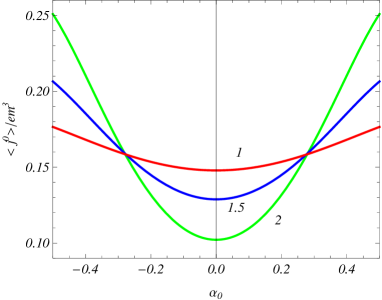
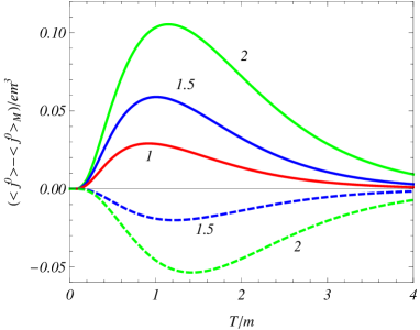
Figure 1: The total charge density as a function of the parameter $\alpha_{0}$ (left panel) and the charge density induced by the string and magnetic flux as a function of the temperature (right panel). The numbers near the curves correspond to the values of the parameter $q$. The graphs on the left panel are plotted for $T/m=1$, $mr=0.25$, and $\mu/m=0.5$. On the right panel, the full and dashed curves correspond to the values $\alpha_{0}=1/2$ and $\alpha_{0}=0$, respectively. For the graphs on the right panel we have taken $\mu/m=0.5$ and $mr=1/8$.

In the discussion above we have assumed that $|\mu|<m$. Now we turn to the case $|\mu|>m$. The charge density is an odd function of the chemical potential and for definiteness we assume that $\mu>m$. In this case the contribution of the antiparticles to the charge density is evaluated in a way similar to that described above and the corresponding expression is given by (3.15) with the lower sign. The total charge density is expressed as

$$\left\langle j^{0}\right\rangle=\left\langle j^{0}\right\rangle_{-}+\frac{eq}{2\pi^{2}}\int_{0}^{\infty}dk\int_{0}^{\infty}d\lambda\ \sum_{j}\lambda\frac{J_{\beta_{j}}^{2}(\lambda r)+J_{\beta_{j}+\epsilon_{j}}^{2}(\lambda r)}{e^{\beta(E-\mu)}+1},$$ (3.39)

where the second term in the right-hand side is the contribution from particles. The integrals over $k$ and $\lambda$ are divided into regions corresponding to $\sqrt{k^{2}+\lambda^{2}}<p_{0}$ and $\sqrt{k^{2}+\lambda^{2}}>p_{0}$ with $p_{0}=\sqrt{\mu^{2}-m^{2}}$ being the Fermi momentum. In the second region we can again use the expansion (3.6). At high temperatures, $T\gg\mu$, the contribution of the states with $E\gg\mu$ dominates and the asymptotic expressions given above are valid.

The situation is essentially changed at low temperatures. Now, in the limit $T\rightarrow 0$, only the contribution of the states with $E\leqslant\mu$ survives and from (3.39) one gets

$$\left\langle j^{0}\right\rangle_{T=0}=\frac{eqp_{0}^{3}}{2\pi^{2}}\ \sum_{j}\int_{0}^{1}dx\,x\sqrt{1-x^{2}}\left[J_{\beta_{j}}^{2}(p_{0}rx)+J_{\beta_{j}+\epsilon_{j}}^{2}(p_{0}rx)\right].$$ (3.40)

The integral in this expression is expressed in terms of the hypergeometric function ${}_{1}F_{2}(a;b,c;x)$. The appearance of the nonzero charge density at zero temperature is related to the presence of particles filling the states with the energies $m\leqslant E\leqslant\mu$. In the case $\mu<0$ we would have antiparticles. In the absence of the planar angle deficit and magnetic flux ($q=1$, $\alpha=0$), the summation over $j$ in (3.40) gives 2 and for the charge density we obtain the standard expression:

$$\left\langle j^{0}\right\rangle_{\mathrm{M},T=0}=\frac{ep_{0}^{3}}{3\pi^{2}}.$$ (3.41)

An alternative expression for the charge density at zero temperature is obtained from (3.40) by using the relation [36]

$$J_{\beta_{j}}^{2}(u)=\frac{1}{2\pi i}\int_{c-i\infty}^{c+i\infty}\frac{dt}{t}e^{t/2-u^{2}/t}I_{\beta_{j}}(u^{2}/t),$$ (3.42)

where $c$ is a positive number. With this relation, the series over $j$ is expressed in terms of the function (3.11). By making use of the representation (3.12) for $F(q,\alpha_{0},x)$, we can see that the contribution coming from the first term in the square brackets of (3.12) gives the charge density $\left\langle j^{0}\right\rangle_{\mathrm{M},T=0}$. In the remaining part, the integral over $t$ is expressed in terms of the Bessel function with the help of the formula

$$\frac{1}{2\pi i}\int_{c-i\infty}^{c+i\infty}\frac{dt}{t}e^{t/2-2b^{2}x^{2}/t}=J_{0}(2bx).$$ (3.43)

This formula is obtained by using the integral representation of the Bessel function from [36] (page 176, formula (1)) deforming the integration contour in the complex plane $t$. The remaining integral is of the form $\int_{0}^{1}dx\,x\sqrt{1-x^{2}}J_{0}(2bx)$. The latter is expressed in terms of the function $J_{3/2}(2b)$ and for the charge density we find the representation

$$\left\langle j^{0}\right\rangle_{T=0} = \left\langle j^{0}\right\rangle_{\mathrm{M},T=0}-\frac{ep_{0}}{2\pi^{2}r^{2}}\ \left[\sum_{k=1}^{[q/2]}(-1)^{k}\frac{c_{k}}{s_{k}^{2}}\cos\left(2\pi k\alpha_{0}\right)g(2p_{0}rs_{k})\right.$$ (3.44)

$$\left.+\frac{q}{\pi}\int_{0}^{\infty}dy\frac{\sinh\left(y\right)h(q,\alpha_{0},2y)}{\cosh(2qy)-\cos(q\pi)}\frac{g(2p_{0}r\cosh y)}{\cosh^{2}y}\right],$$

with the notation

$$g(x)=\cos x-\frac{\sin x}{x}.$$ (3.45)

On the string, for $2|\alpha_{0}|<1-1/q$ one has

$$\left\langle j^{0}\right\rangle_{T=0,r=0}=\frac{ep_{0}^{3}}{3\pi^{2}}\left[1+\ 2h_{0}(q,\alpha_{0})\right].$$ (3.46)

In the case $2|\alpha_{0}|>1-1/q$, the asymptotic behavior near the string is investigated in a way similar to that we have described for $|\mu|<m$. The dominant contribution comes from the last term in the square brackets of (3.44) and we get

$$\left\langle j^{0}\right\rangle_{T=0}\approx\left\langle j^{0}\right\rangle_{\mathrm{M},T=0}+\frac{eqp_{0}^{3}}{2\pi^{2}}\frac{\left[\left(1-2|\alpha_{0}|\right)q+2\right]^{-1}}{\Gamma(1+\left(1-2|\alpha_{0}|\right)q)}\left(p_{0}r\right)^{\left(1-2|\alpha_{0}|\right)q-1}.$$ (3.47)

In this case the charge density diverges on the string and near the string the part induced by the planar angle deficit and magnetic flux dominates the Minkowskian part. Note that the divergence is integrable and the corresponding total charge is finite. At large distances, the charge density induced by the string and magnetic flux exhibits an oscillatory behavior with the amplitude damping as $1/r^{2}$. We just want to point out that in the case $|\mu|<m$ we had an exponential suppression.

In figure 2, the charge density is displayed as a function of the radial coordinate. The full and dashed lines correspond to the values $\alpha_{0}=1/2$ and $\alpha_{0}=0$, respectively. The numbers near the curves present the values of the parameter $q$. The graphs on the left panel are plotted for $T/m=1$ and $\mu/m=0.5$. The graphs on the right panel correspond to the charge density at zero temperature.

Figure 2: The charge density versus the radial coordinate. The full and dashed lines correspond to the values $\alpha_{0}=1/2$ and $\alpha_{0}=0$, respectively. The numbers near the curves present the values of the parameter $q$. The graphs on the left panel are plotted for $T/m=1$ and $\mu/m=0.5$. The graphs on the right panel correspond to the charge density at zero temperature.

Let us consider the total charge, per unit length of the string, at zero temperature, induced by the cosmic string and magnetic flux:

$$\Delta Q_{T=0}=\phi_{0}\int_{0}^{\infty}dr\,r\left[\left\langle j^{0}\right\rangle_{T=0}-\left\langle j^{0}\right\rangle_{\mathrm{M},T=0}\right].$$ (3.48)

The integration over the radial coordinate is reduced to the integral of the form $\int_{0}^{\infty}dx\,g(x)/x$. Note that the separate integrals with $\cos x$ and $\sin x$ from (3.45) diverge at the lower limit. In order to overcome this difficulty, we write the integral as $\lim_{b\rightarrow 0}\int_{0}^{\infty}dx\,xg(x)/(x^{2}+b^{2})$. In this form the separate integrals with $\cos x$ and $\sin x$ are expressed in terms of the error function and taking the limit $b\rightarrow 0$ we can see that $\int_{0}^{\infty}dx\,g(x)/x=-1$. With this result, for the induced charge, one gets

$$\Delta Q_{T=0}=\frac{ep_{0}}{\pi q}h_{2}(q,\alpha_{0}),$$ (3.49)

where the function $h_{n}(q,\alpha_{0})$ is defined by (3.22).

The expression (3.49) can also be obtained by substituting the initial expression (3.40) into (3.48). Though the integrals with separate terms in the square brackets of (3.48) diverge, the induced total charge is finite. For the evaluation of the integral it is convenient to take for $\left\langle j^{0}\right\rangle_{\mathrm{M},T=0}$ the expression which is obtained from (3.40) taking $q=1$ and $\alpha=0$. In order to have a possibility to integrate the terms in (3.48) separately, we write the radial integral as $\int_{0}^{\infty}dr\,=\lim_{\sigma\rightarrow 0}\int_{0}^{\infty}dr\,e^{-\sigma r^{2}}$. Then, the resulting integrals are of the form (3.9) and the charge is expressed in terms of the function (3.11). By using the formula (3.12) for the latter, we can see that the subtraction of the Minkowskian part cancels the contribution of the first term in the square brackets of (3.12). The remaining integral over $x$ is elementary and one gets the result (3.49).

In the discussion above we have considered the charge density as a function of the chemical potential and temperature. From the physical point of view it is of interest also to consider a system with fixed value of the charge. With a fixed charge, the expressions presented above give the chemical potential as a function of the temperature. At high temperatures one has $\left\langle j^{0}\right\rangle\approx\left\langle j^{0}\right\rangle_{\mathrm{M}}\approx e\mu T^{2}/3$ and, hence, for a fixed charge the chemical potential decays as $1/T^{2}$. With decreasing temperature the function $|\mu(T)|$ increases. Its limiting value at zero temperature is obtained from the expressions for the total charge at zero temperature given above.

4 Azimuthal current

Now we turn to the investigation of the current density. The only nonzero component corresponds to the azimuthal current ($\nu=2$ in (2.12)). By taking into account the expression for the mode functions, from (2.14) for the physical components of the current densities of the particles and antiparticles, $\left\langle j_{\phi}\right\rangle_{\pm}=r\left\langle j^{2}\right\rangle_{\pm}$, we get

$$\left\langle j_{\phi}\right\rangle_{\pm}=\frac{eq}{4\pi^{2}}\sum_{\sigma}\epsilon_{j}\frac{\lambda^{2}}{E}\frac{J_{\beta_{j}}(\lambda r)J_{\beta_{j}+\epsilon_{j}}(\lambda r)}{e^{\beta(E\mp\mu)}+1},$$ (4.1)

where the upper and lower signs correspond to the particles and antiparticles respectively and the collective summation is defined by (3.2). Note that for $\mu=0$ the contributions to the total current density from the particles and antiparticles coincide. The current density is an odd periodic function of the magnetic flux with the period equal to the quantum flux.

For the case $|\mu|<m$, again we use the expansion (3.6). This results in the expression

$$\left\langle j_{\phi}\right\rangle_{\pm}=-\frac{eq}{\pi^{2}}\ \sum_{n=1}^{\infty}(-1)^{n}\sum_{j}\ \epsilon_{j}\int_{0}^{\infty}d\lambda\,\lambda^{2}J_{\beta_{j}}(\lambda r)J_{\beta_{j}+\epsilon_{j}}(\lambda r)\int_{0}^{\infty}dk\ \frac{e^{-n\beta(E\mp\mu)}}{E}.$$ (4.2)

By using the integral representation

$$\frac{e^{-n\beta E}}{E}=\frac{2}{\sqrt{\pi}}\int_{0}^{\infty}ds\,e^{-(\lambda^{2}+k^{2}+m^{2})s^{2}-n^{2}\beta^{2}/(4s^{2})},$$ (4.3)

the integration over $k$ is elementary. The integration over $\lambda$ is done with the help of the formula [34]

$$\int_{0}^{\infty}d\lambda\lambda^{2}e^{-\lambda^{2}s^{2}}J_{\beta_{j}}(\lambda r)J_{\beta_{j}+\epsilon_{j}}(\lambda r)=r\epsilon_{j}\frac{e^{-x}}{4s^{4}}\ \left[I_{\beta_{j}}(x)-I_{\beta_{j}+\epsilon_{j}}(x)\right]\ ,$$ (4.4)

where $x=r^{2}/(2s^{2})$. As a result, the current density is expressed as

$$\left\langle j_{\phi}\right\rangle_{\pm}=-\frac{eq}{2\pi^{2}r^{3}}\sum_{n=1}^{\infty}(-1)^{n}e^{\mp n\beta\mu}\int_{0}^{\infty}dx\,xe^{-m^{2}r^{2}/(2x)-(1+n^{2}\beta^{2}/(2r^{2}))x}G(q,\alpha_{0},x),$$ (4.5)

with the notation

$$G(q,\alpha_{0},x)=\sum_{j}\ \left[I_{\beta_{j}}(x)-I_{\beta_{j}+\epsilon_{j}}(x)\right].$$ (4.6)

An equivalent expression for the current density is obtained from (4.5) by making use of the integral representation

$$G(q,\alpha_{0},x) = \frac{4}{q}\sideset{}{{}^{\prime}}{\sum}_{k=1}^{[q/2]}(-1)^{k}s_{k}\sin\left(2\pi k\alpha_{0}\right)e^{x\cos(2\pi k/q)}$$ (4.7)

$$+\frac{4}{\pi}\int_{0}^{\infty}dy\ \frac{g(q,\alpha_{0},2y)\cosh y}{\cosh(2qy)-\cos(q\pi)}e^{-x\cosh{(2y)}},$$

with the notation

$$g(q,\alpha_{0},x)=\sum_{\chi=\pm 1}\chi\cos\left[\left(1/2+\chi\alpha_{0}\right)q\pi\right]\cosh\left[\left(1/2-\chi\alpha_{0}\right)qx\right]\ .$$ (4.8)

The prime on the summation sign in (4.7) means that, in the case where $q$ is an even number, the term with $k=q/2$ should be taken with the coefficient 1/2. Formula (4.7) is obtained by using the representation for the series $\sum_{j}I_{\beta_{j}}(x)$ given in [19]. Substituting (4.7) into (4.5), after integrating over $x$, we obtain

$$\left\langle j_{\phi}\right\rangle_{\pm} =-\frac{4em^{4}r}{\pi^{2}}\sum_{n=1}^{\infty}(-1)^{n}e^{\mp n\beta\mu}$$

$$\times\left[\ \sideset{}{{}^{\prime}}{\sum}_{k=1}^{[q/2]}(-1)^{k}s_{k}\sin\left(2\pi k\alpha_{0}\right)f_{2}\left(m\beta s_{n}(r/\beta,k/q)\right)\right.$$

$$+\left.\frac{q}{\pi}\int_{0}^{\infty}dy\ \frac{\cosh\left(y\right)g(q,\alpha_{0},2y)}{\cosh(2qy)-\cos(q\pi)}f_{2}(m\beta c_{n}(r/\beta,y))\right],$$ (4.9)

where the functions in the arguments of $f_{2}(x)$ are defined by (3.18). In the absence of the conical defect, $q=1$, the above expression reduces to

$$\left\langle j_{\phi}\right\rangle_{\pm} =\frac{4em^{4}r}{\pi^{3}}\sin(\alpha_{0}\pi)\sum_{n=1}^{\infty}(-1)^{n}e^{\mp n\beta\mu}$$

$$\times\int_{0}^{\infty}dy\,\cosh(2\alpha_{0}y)f_{2}\left(m\beta c_{n}(r/\beta,y)\right).$$ (4.10)

Now, by taking into account the expression for the vacuum expectation value of the current density from [17], the total current density is expressed as

$$\left\langle j_{\phi}\right\rangle =-\frac{8em^{4}r}{\pi^{2}}\sideset{}{{}^{\prime}}{\sum}_{n=0}^{\infty}(-1)^{n}\cosh(n\beta\mu)$$

$$\times\left[\ \sideset{}{{}^{\prime}}{\sum}_{k=1}^{[q/2]}(-1)^{k}s_{k}\sin\left(2\pi k\alpha_{0}\right)f_{2}\left(m\beta s_{n}(r/\beta,k/q)\right)\right.$$

$$+\left.\frac{q}{\pi}\int_{0}^{\infty}dy\ \frac{\cosh\left(y\right)g(q,\alpha_{0},2y)}{\cosh(2qy)-\cos(q\pi)}f_{2}\left(m\beta c_{n}(r/\beta,y)\right)\right],$$ (4.11)

where the prime on the sign of the summation over $n$ means that the term $n=0$ should be taken with the coefficient 1/2. This term corresponds to the vacuum expectation value of the current density, $\left\langle j_{\phi}\right\rangle_{0}$.

For a massless field, because of the condition $\mu\leqslant m$, we should also take $\mu=0$. By using the asymptotic expression for the MacDonald function for small values of the argument, the summation over $n$ is reduced to the series of the form $\sideset{}{{}^{\prime}}{\sum}_{n=0}^{\infty}(-1)^{n}\left(n^{2}+x^{2}\right)^{-2}$. The sum of the latter is expressed in terms of the hyperbolic functions and one gets

$$\left\langle j_{\phi}\right\rangle =-\frac{eT}{2\pi r^{2}}\left[\ \sideset{}{{}^{\prime}}{\sum}_{k=1}^{[q/2]}\frac{(-1)^{k}}{s_{k}^{2}}\sin\left(2\pi k\alpha_{0}\right)h(2rTs_{k})\right.$$

$$\left.+\frac{q}{\pi}\int_{0}^{\infty}dy\ \frac{g(q,\alpha_{0},2y)}{\cosh(2qy)-\cos(q\pi)}\frac{h(2rT\cosh y)}{\cosh^{2}y}\right]\ ,$$ (4.12)

where we have introduced the function

$$h(x)=\frac{1+\pi x\coth(\pi x)}{\sinh(\pi x)}.$$ (4.13)

For $|x|\ll 1$ one has $h(x)\approx 2/(\pi x)-7(\pi x)^{3}/180$. The contribution corresponding to the first term in the right-hand side of the latter expression gives the vacuum expectation value of the current density:

$$\left\langle j_{\phi}\right\rangle_{0}=-\frac{eg_{4}(q,\alpha_{0})}{2\pi^{2}r^{3}},$$ (4.14)

where we have defined

$$g_{n}(q,\alpha_{0})=\sideset{}{{}^{\prime}}{\sum}_{k=1}^{[q/2]}(-1)^{k}\frac{\sin\left(2\pi k\alpha_{0}\right)}{s_{k}^{n-1}}+\frac{q}{\pi}\int_{0}^{\infty}dy\ \frac{g(q,\alpha_{0},2y)\cosh^{1-n}y}{\cosh(2qy)-\cos(q\pi)}.$$ (4.15)

The thermal part in the current density for a massless field is given by the right-hand side of (4.12) with the replacement $h(x)\rightarrow h(x)-2/(\pi x)$. This part vanishes on the string. Hence, near the string, $rT\ll 1$, the total current is dominated by the part $\left\langle j_{\phi}\right\rangle_{0}$.

Now we turn to the investigation of the current density in asymptotic regions of the parameters. First we consider the case of a massless field. For $rT\ll 1$, from (4.12), to the leading order one has $\left\langle j_{\phi}\right\rangle\approx\left\langle j_{\phi}\right\rangle_{0}$, with $\left\langle j_{\phi}\right\rangle_{0}$ given by (4.14). This limit corresponds to points close to the string, for a fixed value of the temperature, or to lower temperatures, for fixed $r$. The relative contribution of the thermal effects is suppressed by the factor $(rT)^{4}$. In the opposite limit, $rT\gg 1$, two cases should be considered separately. For $q<2$, in (4.12) the sum over $k$ is absent and the dominant contribution to the integral comes from values of $y$ near the lower limit. Assuming that $\sin(q\pi/2)\gg q/\sqrt{\pi rT}$ ($q$ is not too close to 2), to the leading order one gets

$$\left\langle j_{\phi}\right\rangle\approx\frac{eq(rT)^{3/2}\sin(\alpha_{0}q\pi)}{\pi r^{3}\sin(q\pi/2){e}^{2\pi rT}}.$$ (4.16)

In the case $q>2$, the contribution of the term with $k=1$ dominates and we find

$$\left\langle j_{\phi}\right\rangle\approx\frac{2e\sin\left(2\pi\alpha_{0}\right)}{r^{3}\sin{(\pi/q)}}\frac{(rT)^{2}}{{e}^{2\pi rT\sin{(\pi/q)}}}.$$ (4.17)

In both cases the current density is exponentially suppressed. The expressions (4.16) and (4.17) correspond to high temperatures for fixed $r$ or to large distances from the string for fixed $T$.

For a massive field, in the limit $r\rightarrow 0$ and for $2|\alpha_{0}|<1-1/q$, in the expression of the square brackets in (4.11), corresponding to the finite temperature terms, we can directly put $r=0$:

$$\left\langle j_{\phi}\right\rangle\approx\left\langle j_{\phi}\right\rangle_{0}-\frac{8em^{4}r}{\pi^{2}}g_{0}(q,\alpha_{0})\sum_{n=1}^{\infty}(-1)^{n}\cosh(n\beta\mu)f_{2}\left(nm\beta\right).$$ (4.18)

In the limit $r\rightarrow 0$, for the vacuum expectation value, to the leading order, one has

$$\left\langle j_{\phi}\right\rangle_{0}\approx-\frac{eg_{4}(q,\alpha_{0})}{2\pi^{2}r^{3}}.$$ (4.19)

The latter diverges on the string and, hence, near the string the total current is dominated by the zero temperature part.

In the case $2|\alpha_{0}|>1-1/q$ and in the limit $r\rightarrow 0$, the integral over $y$ in (4.11), corresponding to the the thermal part ($n\neq 0$), diverges and we cannot directly put $r=0$. We note that in this case the dominant contribution to the integral over $y$ comes from large values of $y$. Replacing the integrand by its asymptotic form for large $y$, the integral is evaluated in terms of the MacDonald function and one gets

$$\left\langle j_{\phi}\right\rangle \approx \left\langle j_{\phi}\right\rangle_{0}+\frac{2^{3/2}}{\pi^{2}}\mathrm{sgn}(\alpha_{0})\frac{eqm^{3}(mr/\sqrt{2})^{\left(1-2|\alpha_{0}|\right)q}}{\Gamma(1/2+\left(1/2-|\alpha_{0}|\right)q)}$$ (4.20)

$$\times\sum_{n=1}^{\infty}(-1)^{n}\cosh(n\beta\mu)f_{3/2+\left(1/2-|\alpha_{0}|\right)q}(nm\beta).$$

For the vacuum expectation value we have the asymptotic expression (4.19) and, again, it dominates for points near the string.

Now let us discuss the asymptotic expressions for the current density at low and high temperatures. At low temperatures, $T\ll m,r^{-1}$, and for $2|\alpha_{0}|<1-1/q$, in (4.11), for the terms corresponding to the thermal corrections we can put $r/\beta=0$ in the arguments of the functions $f_{2}(x)$. By using the asymptotic expression of the MacDonald function for large arguments we find

$$\left\langle j_{\phi}\right\rangle\approx\left\langle j_{\phi}\right\rangle_{0}+\frac{4em^{4}re^{-\left(m-|\mu|\right)\beta}}{\sqrt{2}\pi^{3/2}\left(m\beta\right)^{5/2}}g_{0}(q,\alpha_{0}).$$ (4.21)

In the case $2|\alpha_{0}|\geqslant 1-1/q$ and for low temperatures we cannot directly put $r/\beta=0$ in the integrand of (4.11) for the thermal part because the resulting integral is divergent. At low temperatures the integral is dominated by the contribution of large $y$. By using the asymptotic expression for the integrand, we get

$$\left\langle j_{\phi}\right\rangle\approx\left\langle j_{\phi}\right\rangle_{0}-\frac{eqm(mr/\sqrt{2})^{\left(1-2|\alpha_{0}|\right)q}}{\pi^{3/2}\Gamma(1/2+\left(1/2-|\alpha_{0}|\right)q)}\frac{\mathrm{sgn}(\alpha_{0})e^{-(m-|\mu|)\beta}}{\beta^{2}(m\beta)^{\left(1/2-|\alpha_{0}|\right)q}}.$$ (4.22)

Hence, under the condition $|\mu|<m$, at low temperatures the thermal corrections are exponentially suppressed.

In order to investigate the high temperature asymptotic behavior, it is convenient to present the current density (4.9) in an alternative form by using the relation (3.29). The corresponding expression reads

$$\left\langle j_{\phi}\right\rangle = -\frac{16eTr}{(2\pi)^{3/2}}\sum_{n=-\infty}^{+\infty}b_{n}^{3}(T)\left[\ \sideset{}{{}^{\prime}}{\sum}_{k=1}^{[q/2]}(-1)^{k}s_{k}\sin\left(2\pi k\alpha_{0}\right)f_{3/2}(2rs_{k}b_{n}(T))\right.$$ (4.23)

$$\left.+\frac{q}{\pi}\int_{0}^{\infty}dy\ \frac{\cosh\left(y\right)g(q,\alpha_{0},2y)}{\cosh(2qy)-\cos(q\pi)}f_{3/2}(2r\cosh yb_{n}(T))\right],$$

where $b_{n}(T)$ is defined by (3.31). Note that $f_{3/2}(x)=\sqrt{\pi/2}x^{-3}(1+x)e^{-x}$. In (4.23) we can also write $\sum_{n=-\infty}^{+\infty}\cdots=2\sum_{n=0}^{\infty}\mathrm{Re}\left[\cdots\right]$. For a massless fermionic field, because of the condition $|\mu|\leqslant m$, we should also take $\mu=0$ and one gets

$$\left\langle j_{\phi}\right\rangle =-\frac{eT}{\pi r^{2}}\sum_{n=0}^{\infty}\left[\ \sideset{}{{}^{\prime}}{\sum}_{k=1}^{[q/2]}(-1)^{k}\sin\left(2\pi k\alpha_{0}\right)\frac{1+2\pi(2n+1)s_{k}Tr}{s_{k}^{2}e^{2\pi(2n+1)s_{k}Tr}}\right.$$

$$+\left.\frac{q}{\pi}\int_{0}^{\infty}dy\ \frac{g(q,\alpha_{0},2y)}{\cosh(2qy)-\cos(q\pi)}\frac{1+2\pi(2n+1)Tr\cosh y}{e^{2\pi(2n+1)Tr\cosh y}\cosh^{2}y}\right].$$ (4.24)

At high temperatures one has $r|b_{n}(T)|\gg 1$, and the dominant contribution in (4.23) comes from the terms $n=0$ and $n=-1$. For $q>2$ the leading contribution comes from the $k=1$ term in the right-hand side and we get

$$\left\langle j_{\phi}\right\rangle\approx\ \frac{2eT^{2}\sin\left(2\pi\alpha_{0}\right)}{r\sin{(\pi/q)}}\cos(2\mu r\sin{(\pi/q)})e^{-2\pi rT\sin{(\pi/q)}}\ .$$ (4.25)

For $q<2$, the sum over $k$ in (4.23) is absent. At high temperatures, the dominant contribution to the integral over $y$ comes from the region near the lower limit of the integration. Assuming that $\sin(\pi q/2)\gg 1/\sqrt{rT}$ ($q$ is not too close to 2), to the leading order one finds

$$\left\langle j_{\phi}\right\rangle\approx\frac{eq\sin(\alpha_{0}q\pi)T^{3/2}}{\pi\sin(\pi q/2)r^{3/2}}\cos(2\mu r)e^{-2\pi rT}.$$ (4.26)

Hence, at high temperatures, $T\gg m,r^{-1}$, the current density is exponentially small.

At large distances from the string, in (4.23) the contribution from the terms with $k=1$ and $n=-1,0$ dominate and for $q>2$ one gets

$$\left\langle j_{\phi}\right\rangle\approx\frac{2eT}{\pi r}\frac{\sin\left(2\pi k\alpha_{0}\right)}{\sin(\pi/q)}\mathrm{Re\,}[b_{0}(T)\ e^{-2rb_{0}(T)\sin(\pi/q)}].$$ (4.27)

For $q<2$ the sum over $k$ in (4.23) is absent and at large distances the dominant contribution comes from the region near the lower limit of the integral over $y$. Assuming that $rT\gg\sin^{-2}(\pi q/2)$, to the leading order we find

$$\left\langle j_{\phi}\right\rangle\approx\frac{eqT}{\pi^{3/2}r^{2}}\frac{\sin(\pi q\alpha_{0})}{\sin(\pi q/2)}\mathrm{Re\,}[(rb_{0}(T))^{1/2}e^{-2rb_{0}(T)}]\ .$$ (4.28)

In both cases one has an exponential decay.

In figure 3, for a massless field with $\mu=0$, we have plotted the azimuthal current density as a function of the parameter $\alpha_{0}$ (left panel) and as a function of the temperature (right panel). The numbers near the curves correspond to the values of $q$. The graphs on the left panel are plotted for $rT=0.25$ and on the right panel for $\alpha_{0}=0.25$.

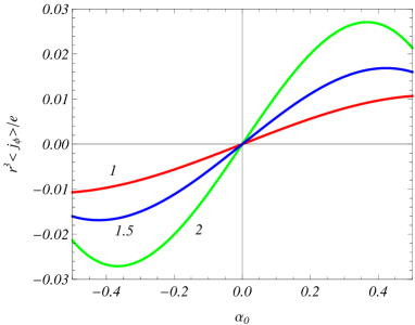
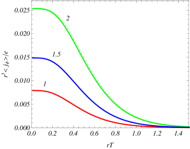
Figure 3: The azimuthal current density for a massless field with zero chemical potential as a function of $\alpha_{0}$ (left panel) and as a function of the temperature (right panel). The numbers near the curves correspond to the values of $q$. For the graphs on the left panel $rT=0.25$ and for the right panel $\alpha_{0}=0.25$.

Now let us consider the azimuthal current density in the case $|\mu|>m$. The current density is an even function of the chemical potential and it suffices to consider positive values of $\mu$. In this case the contribution of the antiparticles to the current density is evaluated in a way similar to that we have described for $\mu<m$. This contribution is given by (4.9) with the lower sign. For the total current one gets

$$\left\langle j_{\phi}\right\rangle=\left\langle j_{\phi}\right\rangle_{0}+\left\langle j_{\phi}\right\rangle_{-}+\frac{eq}{\pi^{2}}\int_{0}^{\infty}dk\int_{0}^{\infty}d\lambda\ \sum_{j}\epsilon_{j}\frac{\lambda^{2}}{E}\frac{J_{\beta_{j}}(\lambda r)J_{\beta_{j}+\epsilon_{j}}(\lambda r)}{e^{\beta(E-\mu)}+1},$$ (4.29)

where the last term is the part coming from the particles. At high temperatures, $T\gg\mu$, the dominant contribution comes from the states with energies $E\gg\mu$ and the asymptotic behavior of the current density is similar to that we have described above for the case $\mu<m$. At zero temperature, taking the limit $T\rightarrow 0$ in (4.29), we obtain

$$\left\langle j_{\phi}\right\rangle_{T=0}=\left\langle j_{\phi}\right\rangle_{0}+\frac{eq}{\pi^{2}}\int_{0}^{p_{0}}du\,\frac{u^{3}}{\sqrt{u^{2}+m^{2}}}\int_{0}^{1}dx\frac{x^{2}}{\sqrt{1-x^{2}}}\sum_{j}\epsilon_{j}J_{\beta_{j}}(urx)J_{\beta_{j}+\epsilon_{j}}(urx).$$ (4.30)

The second term in the right-hand side is the contribution from the particles filling the states with the energies $E\leqslant\mu$.

For the further transformation of the zero temperature current density, in (4.30) we use the relation

$$\epsilon_{j}J_{\beta_{j}}(z)J_{\beta_{j}+\epsilon_{j}}(z)=\frac{1}{z}\left(\epsilon_{j}\beta_{j}-\frac{1}{2}z\partial_{z}\right)J_{\beta_{j}}^{2}(z),$$ (4.31)

and the integral representation (3.42) for the square of the Bessel function. Next, by taking into account that

$$\left(\epsilon_{j}\beta_{j}-z\partial_{z}/2\right)e^{-z}I_{\beta_{j}}(z)=ze^{-z}\left[I_{\beta_{j}}(z)-I_{\beta_{j}+\epsilon_{j}}(z)\right],$$ (4.32)

the series over $j$ is expressed in terms of the function (4.6). By using the representation for the latter given by (4.7), the integral over $t$ coming from (3.42) is expressed in terms of the Bessel function $J_{1}(2urxb)$, where $b=s_{k}$ and $b=\cosh y$ for the first and second terms in the right-hand side of (4.7), respectively. After the integration over $x$, we find

$$\left\langle j_{\phi}\right\rangle_{T=0} = \left\langle j_{\phi}\right\rangle_{0}-\frac{ep_{0}^{3}}{\pi^{2}}\left[\sideset{}{{}^{\prime}}{\sum}_{k=1}^{[q/2]}(-1)^{k}\sin\left(2\pi k\alpha_{0}\right)f(p_{0}rs_{k},m/p_{0})\right.$$ (4.33)

$$\left.+\frac{q}{\pi}\int_{0}^{\infty}dy\ \frac{f(p_{0}r\cosh y,m/p_{0})}{\cosh(2qy)-\cos(q\pi)}g(q,\alpha_{0},2y)\right],$$

with the notation

$$f(a,b)=\frac{1}{a}\int_{0}^{1}dx\,\frac{x^{2}g(2ax)}{\sqrt{x^{2}+b^{2}}}.$$ (4.34)

Here, the function $g(x)$ is defined by (3.45). For a massless field one has

$$f(a,0)=a^{-3}\sin^{2}a\left(a\cot a-1\right).$$ (4.35)

The second term in the right-hand side of (4.33) vanishes on the string, whereas the first one diverges as $1/r^{3}$. Hence, near the string the current density is dominated by the vacuum expectation value. In order to find the asymptotic behavior of (4.33) at large distances, $p_{0}r\gg 1$, we note that for $a\gg 1$ one has

$$f(a,b)\approx\frac{1}{2a^{2}}\frac{\sin(2a)}{\sqrt{1+b^{2}}}.$$ (4.36)

Hence, at large distances, the contribution in the current density coming form the particles exhibits a damping oscillatory behavior with the amplitude decaying as $1/r^{2}$. The vacuum expectation value decays as $1/r^{3}$ for a massless field and exponentially for a massive field and, hence, it is subdominant at large distances.

In figure 4, for a massless field, we have plotted the azimuthal current density at zero temperature and $\mu>0$ (full curves), as a function of the radial coordinate, for various values of the parameter $q$ (numbers near the curves, the curve in the middle corresponds to $q=1.5$). For the value of $\alpha_{0}$ we have taken $\alpha_{0}=0.25$. The dashed curves correspond to the vacuum expectation value of the current density, $\left\langle j_{\phi}\right\rangle_{0}$, for the same values of $q$.

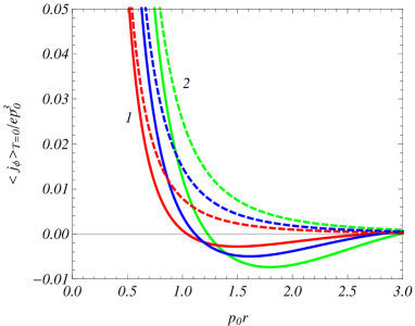
Figure 4: The zero temperature azimuthal current density for a massless field with $\mu>0$, as a function of the radial coordinate (full curves). The numbers near the curves correspond to the values of $q$. The graphs are plotted for $\alpha_{0}=0.25$. The dashed curves correspond to the vacuum expectation value of the azimuthal current.

5 Conclusion

In this paper, we have investigated the combined effects of the planar angle deficit and the magnetic flux on the charge and current densities for a massive fermionic field with nonzero chemical potential at thermal equilibrium. For the evaluation of the corresponding expectation values the direct summation over a complete set of fermionic modes is used. These densities are decomposed into the vacuum expectation values and finite temperature contributions, coming from the particles and antiparticles.

For the charge density the vacuum expectation value vanishes and the expectation value for the particles and antiparticles in the case $|\mu|\leqslant m$ are given by (3.15), where $\left\langle j^{0}\right\rangle_{\mathrm{M}\pm}$ is the corresponding quantity in the absence of the planar angle deficit and the magnetic flux. The charge density is an even periodic function of the magnetic flux with period equal to the quantum flux. For the zero chemical potential the contributions from the particles and antiparticles cancel each other and the total charge density, given by (3.19), vanishes. An alternative expression for the charge density, convenient for the investigation of high temperature regime, is provided by (3.32). The charge density is finite on the string for the values of the magnetic flux in the range $2|\alpha_{0}|\leqslant 1-1/q$ and diverges as $r^{\left(1-2|\alpha_{0}|\right)q-1}$ for $2|\alpha_{0}|>1-1/q$. This divergence is integrable and the total charge induced by the cosmic string and magnetic flux is finite (see (3.24)). At large distances from the string and for $|\mu|\leqslant m$, the asymptotic expressions for the charge density in the cases $q>2$ and $q<2$ are given by (3.37) and (3.38), respectively. In this limit, the contributions in the charge density induced by the string and magnetic flux are exponentially small. At low temperatures the charge density is suppressed by the factor $e^{-\beta(m-|\mu|)}$. At high temperatures, the contribution to the charge density coming from the string and magnetic flux is suppressed by the factor $e^{-2\pi rT\sin(\pi/q)}$ for $q>2$ and by the factor $e^{-2\pi rT}$ for $q<2$. In this limit the charge density is dominated by the Minkowskian part with the high temperature asymptotic given by (3.34).

We have also investigated the charge density for the case $|\mu|>m$. By taking into account that the charge density is an odd function of the chemical potential, for definiteness, it is assumed that $\mu>0$. At high temperatures, the dominant contribution to the expectation values comes from the states with the energies $E\gg|\mu|$ and the corresponding behavior is similar to that for the case $\mu<m$. The behavior of the charge density is essentially changed at low temperatures. Now, in the limit $T\rightarrow 0$ the charge density does not vanish and the corresponding limiting value is given by (3.40). The appearance of the nonzero charge density at zero temperature is related to the presence of particles filling the states with the energies $m\leqslant E\leqslant\mu$. An alternative expression for the charge density at zero temperature is provided by (3.44) where the Minkowskian part is given by (3.41). The zero temperature charge density is finite on the string for $2|\alpha_{0}|\leqslant 1-1/q$ and diverges for $2|\alpha_{0}|>1-1/q$. The divergence is integrable and the total charge induced by the cosmic string and magnetic flux is finite and is given by the expression (3.49). At large distances from the string, the zero temperature charge density induced by the string and magnetic flux exhibits an oscillatory behavior with the amplitude decaying as $1/r^{2}$. This behavior is in contrast with the case $|\mu|<m$ where we had an exponential suppression.

The only nonzero component of the expectation value for the current density corresponds to the current along the azimuthal direction. This current vanishes in the absence of the magnetic flux and is an odd periodic function of the latter with the period equal to the quantum flux. The azimuthal current density is an even function of the chemical potential. For the zero chemical potential, the contributions to the total current density from the particles and antiparticles coincide. Similar to the case of the charge density, in the case $|\mu|\leqslant m$, for the azimuthal current we have provided two equivalent representations, (4.11) and (4.23). The first one is convenient for the investigation of the asymptotic behavior near the string and at low temperatures, whereas the second one is well adapted for the consideration of the asymptotics at large distances and high temperatures. For a massless fermionic field the corresponding expressions are simplified to (4.12) and (4.24). The contribution in the current density coming from particles and antiparticles vanish on the string whereas the vacuum expectation value diverges as $r^{-3}$ and near the string the latter dominates in the total current. At large distances from the string, $r\gg T^{-1},m^{-1}$, and for $|\mu|<m$, the leading terms in the asymptotic expansions over the distance from the string are given by (4.27) and (4.28) and the current density decays exponentially. At low temperatures, under the condition $|\mu|<m$, the finite temperature part in the current density is suppressed by the factor $e^{-(m-|\mu|)/T}$ and the vacuum expectation value dominates. At high temperatures, the leading terms in the expectation value of the current density are given by the expressions (4.25) and (4.26) for the cases $q>2$ and $q<2$, respectively. In both cases the current density is exponentially small. At high temperatures the contribution of the states with the energies $E\gg\mu$ dominates and this behavior is valid for the case $|\mu|>m$ as well. This is not the case at low temperatures. For $|\mu|>m$ and in the limit $T\rightarrow 0$, the current density has two contributions. The first one corresponds to the vacuum expectation value and the second one comes from the particles in the case $\mu>0$ and from the antiparticles for $\mu<0$, filling the states with the energies $m\leqslant E\leqslant|\mu|$. The current density is an even function of the chemical potential and we have considered the case $\mu>m$. The two alternative representations for the azimuthal current at zero temperature are given by (4.30) and (4.33). The part in the zero temperature current density coming from the particles vanishes on the string and for points near the string the vacuum expectation value dominates. At large distances from the string, $p_{0}r\gg 1$, the contribution in the zero temperature current density coming form the particles exhibits a damping oscillatory behavior with the amplitude decaying as $1/r^{2}$ and it dominates over the vacuum current.

References

• [1] N.B. Nielsen and P. Olesen, Nucl. Phys. B 61, 45 (1973).
• [2] D. Garfinkle, Phys. Rev. D 32, 1323 (1985).
• [3] B. Linet, Phys. Lett. B 124, 240 (1987).
• [4] A. Vilenkin and E.P.S. Shellard, Cosmic Strings and Other Topological Defects (Cambridge University Press, Cambridge, 1994).
• [5] S. Sarangi and S.H.H. Tye, Phys. Lett. B 536, 185 (2002); E.J. Copeland, R.C. Myers, and J. Polchinski, JHEP 06, 013 (2004); G. Dvali and A. Vilenkin, JCAP 0403, 010 (2004).
• [6] D.R. Nelson, Defects and Geometry in Condensed Matter Physics (Cambridge University Press, Cambridge, 2002); G.E. Volovik, The Universe in a Helium Droplet (Clarendon, Oxford, 2003).
• [7] J.S. Dowker, Phys. Rev. D 36, 3095 (1987); J.S. Dowker, Phys. Rev. D 36, 3742 (1987).
• [8] M.E.X. Guimarães and B. Linet, Commun. Math. Phys. 165, 297 (1994).
• [9] J. Spinelly and E.R. Bezerra de Mello, Class. Quantum Grav. 20 874, (2003); J. Spinelly and E.R. Bezerra de Mello, Int. J. Mod. Phys. A 17, 4375 (2002).
• [10] J. Spinelly and E.R. Bezerra de Mello, Int. J. Mod. Phys. D 13, 607 (2004).
• [11] J. Spinelly and E. R. Bezerra de Mello, JHEP 09, 005 (2008).
• [12] Yu.A. Sitenko and N.D. Vlasii, Class. Quantum Grav. 29, 095002 (2012).
• [13] M.G. Alford and F. Wilczek, Phys. Rev. Lett. 62, 1071 (1989); K. Jones-Smith, H. Mathur, and T. Vachaspati, Phys. Rev. D 81, 043503 (2010); Y.-Z. Chu, H. Mathur, and T. Vachaspati, Phys. Rev. D 82, 063515 (2010); D.A. Steer and T. Vachaspati, Phys. Rev. D 83, 043528 (2011).
• [14] L. Sriramkumar, Class. Quantum Grav. 18, 1015 (2001).
• [15] Yu.A. Sitenko and N.D. Vlasii, Class. Quantum Grav. 26, 195009 (2009).
• [16] E.R. Bezerra de Mello, Class. Quantum Grav. 27, 095017 (2010).
• [17] E.R. Bezerra de Mello and A. A. Saharian, Eur. Phys. J. C 73, 2532 (2013).
• [18] E.A.F. Bragança, H.F. Santana Mota, and E. R. Bezerra de Mello, arXiv:1410.1511.
• [19] E.R. Bezerra de Mello, V.B. Bezerra, A.A. Saharian, and V.M. Bardeghyan, Phys. Rev. D 82, 085033 (2010).
• [20] S. Bellucci and A.A. Saharian, Phys. Rev. D 82, 065011 (2010); S. Bellucci and A.A. Saharian, Phys. Rev. D 87, 025005 (2013).
• [21] S. Bellucci, A.A. Saharian, and H.A. Nersisyan, Phys. Rev. D 88, 024028 (2013).
• [22] E.R. Bezerra de Mello, A.A. Saharian, and V. Vardanyan, arXiv:1410.2860.
• [23] A. Mohammadi, E.R. Bezerra de Mello, and A.A. Saharian, arXiv:1407.8095.
• [24] E.R. Bezerra de Mello, V.B. Bezerra, A.A. Saharian, and H.H. Harutyunyan, arXiv:1411.1258.
• [25] E.R. Bezerra de Mello and A.A. Saharian, Phys. Rev. D 87, 045015 (2013).
• [26] S. Bellucci, E.R. Bezerra de Mello and A.A. Saharian, Phys. Rev. D 89, 085002 (2014).
• [27] P.C.W. Davies and V. Sahni, Class. Quantum Grav. 5, 1 (1988).
• [28] B. Linet, Class. Quantum Grav. 9, 2429 (1992).
• [29] V.P. Frolov, A. Pinzul and A.I. Zelnikov, Phys. Rev. D 51, 2770 (1995).
• [30] M.E.X. Guimarães, Class. Quantum Grav. 12, 1705 (1995).
• [31] B. Linet, Class. Quantum Grav. 13, 97 (1996).
• [32] P. de Sousa Gerbert and R. Jackiw, Commun. Math. Phys. 124, 229 (1989); P. de Sousa Gerbert, Phys. Rev. D 40, 1346 (1989); Yu.A. Sitenko, Ann. Phys. 282, 167 (2000).
• [33] R. Jackiw, A.I. Milstein, S.-Y. Pi, and I.S. Terekhov, Phys. Rev. B 80, 033413 (2009); A.I. Milstein and I.S. Terekhov, Phys. Rev. B 83, 075420 (2011).
• [34] I.S. Gradshteyn and I.M. Ryzhik, Table of Integrals, Series and Products (Academic Press, New York, 1980).
• [35] S. Bellucci and A.A. Saharian, Phys. Rev. D 79, 085019 (2009).
• [36] G.N. Watson, A Treatise on the Theory of Bessel Functions (Cambridge University Press, Cambridge, 1966).