Robust Recovery of Stream of Pulses using Convex Optimization

Abstract

This paper considers the problem of recovering the delays and amplitudes of a weighted superposition of pulses. This problem is motivated by a variety of applications, such as ultrasound and radar. We show that for univariate and bivariate stream of pulses, one can recover the delays and weights to any desired accuracy by solving a tractable convex optimization problem, provided that a pulse-dependent separation condition is satisfied. The main result of this paper states that the recovery is robust to additive noise or model mismatch.

1 Introduction

In this paper we consider signals of the form

$$y(t)=\sum_{m}c_{m}K_{\sigma}\left(t-t_{m}\right),$$ (1.1)

where $K_{\sigma}(t):=K(\sigma^{-1}t)$ and $\sum_{m}|c_{m}|<\infty$. We assume that the kernel (pulse) $K$ and the scaling $\sigma>0$ are known, whereas the delays $\left\{t_{m}\right\}$ and the real amplitudes $\left\{c_{m}\right\}$ are unknown. The delayed versions of the kernel, $\left\{K_{\sigma}(t-t_{m})\right\}_{m}$, are often referred to as atoms. In Section 2 we discuss specific requirements for $K$.

An alternative representation of the signal in (1.1) is

$$y(t)=\left(K_{\sigma}\ast x\right)(t)=\int_{\mathbb{R}}K_{\sigma}(t-s)dx(s),$$

where

$$x(t)=\sum_{m}c_{m}\delta_{t_{m}}(t),$$ (1.2)

and $\delta_{t}$ denotes a Dirac measure. This model is quite common in a number of engineering applications such as ultrasound [50, 53, 5], radar [2] and more (see e.g. [51, 22, 42]). In these applications, we transmit a pulse and measure the received echoes. This formulation resembles the problem of super-resolution that has received considerable attention recently [13, 12, 28, 36]. However, our problem is defined on $\mathbb{R}^{n}$ whereas the super-resolution problem is defined on the n-dimensional torus. Additionally, we are not restricted to band-limited kernels and can deal with a broader family of convolution kernels as presented in Definition 2.3.

Let $\hat{x}$, $\hat{y}$ and $\hat{K}_{\sigma}$ be the Fourier transforms of $x,y$ and $K_{\sigma}$, respectively. A naive approach will aim to recover $x$ through the relation $\hat{x}=\hat{y}/\hat{K}_{\sigma}$. However, since $x$ is a Dirac sequence and consequently $\hat{x}$ is non-vanishing, this approach will not work for practical decaying kernels even if $\hat{K}_{\sigma}$ is non-vanishing. A well-known approach to decompose the signal into its atoms is by using parametric methods such as MUSIC and matrix pencil [44, 32, 40, 43]. These methods do not assume any structure on the signal besides sparsity. However, they tend to be unstable in the presence of noise or model mismatch due to sensitivity of polynomial root finding. As far as we know, they have no guarantees for their robustness (although significant progress has been made recently for the particular case of super-resolution [37, 34]).

An alternative way is to utilize compressed sensing and sparse representations theorems, relying on the sparsity of the signal in a discrete basis (e.g. [26, 21]). Evidently, signals that have sparse representation in a continuous dictionary might not have sparse representation after discretization [15]. An obvious technique to alleviate this basis mismatch is by fine discretization. However, the aforementioned fields cannot explain the success of $\ell_{1}$ minimization or greedy algorithms as the dictionaries have high coherence [45].

Recently, a number of works suggested sparsity-promoting convex optimization techniques over the continuum. In these works, the notion of coherence does not play any role. Particularly, it was suggested to recast Total-Variation (TV) and atomic norm minimization as semi-definite programs (SDP) in order to recover point sources from low-resolution data on the line [13, 12], and on the sphere [7, 8, 9], or for line spectral estimation [10, 47, 46]. Similar approach was applied to the recovery of non-uniform splines from their projection onto algebraic polynomial spaces [6, 20] (see also [18, 1]).

We follow this line of work and employ TV minimization techniques to recover the delays and amplitudes from the measured data $y(t)$. The aforementioned works exploit the special structure of trigonometric and algebraic polynomials to recast the dual of the infinite dimensional problem as a finite SDP, based on the Riesz-Fejer Thereom [23] (see also an SDP approach for the primal problem in [19]). However, as far as we know, there is no tractable algorithm solving the TV minimization on $\mathbb{R}$. Therefore, in practice, we consider a sampled version of $y(t)$, which reduces the infinite dimensional TV minimization to a finite $\ell_{1}$ minimization problem. The continuous nature of our analysis guarantees that the results hold for any discretization of the parameter space, with no dependence on the dictionary coherence (see also [48]). The behavior of the discrete optimization problem solution, when the underlying signal is defined on the continuum (as typically occurs in practical applications) is analyzed in detail in [24, 25, 45].

The outline of this paper is as follows. After this introduction section, Section 2 presents our main results. In Theorems 2.7 and 2.11 we show that a sufficient condition for a successful recovery is that the delays are sufficiently separated. We further establish in Theorem 2.12 that recovery via $\ell_{1}$ minimization is robust to additive noise or model mismatch, and the error is proportional to the noise level. We note that we make no statistical assumptions on the noise so our results are quite general. Section 3, which is the main body of this paper, is dedicated to the presentation of proofs. In Section 4 we present the results of numerical experiments we have conducted, and in Section 5 we draw conclusions and discuss the implications of our results.

2 Main Results

In this section we present our main results. For the benefit of the reader we provide the formal definition of Total Variation (TV) norm (see [41]):

Definition 2.1.

Let $\mathcal{B}(A)$ be the Borel $\sigma$-Algebra on a space $A$, and denote by $\mathcal{M}(A)$ the associated space of real Borel measures. The Total Variation (TV) of a real Borel measure $v\in\mathcal{M}(A)$ over a set $B\in\mathcal{B}(A)$ is defined by

$$|v|(B)=\sup\sum_{k}|v(B_{k})|,$$

where the supremum is taken over all partitions of $B$ into countable disjoint subsets. The total variation $|v|$ is a non-negative measure on $\mathcal{B}(A)$, and the Total Variation (TV) norm of $v$ is defined as

$$\|v\|_{TV}=|v|(A).$$

The TV norm of a signed measure can be interpreted as the generalization of $\ell_{1}$ norm to the real line. For a discrete measure of the form of (1.2), it is easy to see that

$$\|x\|_{TV}=\sum_{m}|c_{m}|.$$

Next we need the following definitions:

Definition 2.2.

A set of points $T\subset\mathbb{R}$ is said to satisfy the minimal separation condition for a kernel dependent $\nu>0$ and a given $\sigma>0$ if

$$\Delta:=\min_{t_{i},t_{j}\in T,t_{i}\neq t_{j}}\left|t_{i}-t_{j}\right|\geq\nu\sigma.$$

Definition 2.3.

A kernel $K$ is admissible if it has the following properties:

1. $K\in\mathcal{C}^{3}\left(\mathbb{R}\right)$, is real and even.

2. Global property: There exist constants $C_{\ell}>0,\ell=0,1,2,3$ such that $\left|K^{\left(\ell\right)}\left(t\right)\right|\leq\ C_{\ell}/\left({1+t^{2}}\right)$ , where $K^{\left(\ell\right)}\left(t\right)$ denotes the $\ell^{th}$ derivative of $K$.

3. Local property: There exist constants $\varepsilon,\beta>0$ such that

   1. $K(t)>0$ for all $|t|\leq\varepsilon$ and $K(t)<K(\varepsilon)$ for all $|t|>\varepsilon$,

   2. $K^{\left(2\right)}\left(t\right)<-\beta$ for all $|t|\leq\varepsilon$.

Remark 2.4.

By the Taylor Remainder theorem, for any $0<t\leq\varepsilon$, there exists $0<\xi\leq t$ such that

$$K^{(1)}(t)=K^{(1)}(0)+tK^{(2)}(\xi)=tK^{(2)}(\xi)<0.$$

Hence, the local property implies that $K$ is monotonically decreasing in $t\in(0,\varepsilon)$.

Remark 2.5.

The global property in Definition 2.3 can be somewhat weakened to $\left|K^{\left(\ell\right)}\left(t\right)\right|\leq C_{\ell}/(1+|t|^{1+s})$ for some $s>0$. In this case, the separation condition would become dependent on $s$.

Remark 2.6.

Two prime examples for an admissible kernel are the Gaussian kernel, $K\left(t\right)=e^{-t^{2}/2}$ and the Cauchy kernel, $K(t)=1/\left({1+t^{2}}\right)$. The reader can readily verify that both are admissible. Table 1 presents the numerical constants $C_{\ell}$, $\ell=0,1,2,3$ for both kernels.

Our first theorem states that one can recover the unknown delays and amplitudes of a given stream of pulses (1.1) by simply minimizing the TV norm of (1.2).

Theorem 2.7.

For any admissible kernel $K$, there exists $\nu>0$ such that for any $\sigma>0$, the delays and amplitudes of any signal $y$ of the form (1.1), with delays $T:=\{t_{m}\}$ satisfying the separation condition of Definition 2.2, can be recovered as the unique solution of

$$\min_{\tilde{x}\in\mathcal{M}(\mathbb{R})}\left\|\tilde{x}\right\|_{TV}\quad\mbox{subject to}\quad y(t)=\int_{\mathbb{R}}K_{\sigma}(t-s)d\tilde{x}\left(s\right),$$ (2.1)

where $\mathcal{M}(\mathbb{R})$ is the space of signed Borel measures on $\mathbb{R}$.

Remark 2.8.

We note that the feasible set of the optimization problem (2.1) is one-element if and only if the Fourier transform of $K_{\sigma}$ is not vanishing identically on an interval. In this sense, Theorem 2.7 is trivial for kernels whose Fourier transform does not vanish identically on an interval, such as the Gaussian and Cauchy kernels and the signal can be recovered linearly by $\hat{y}=\hat{K}_{\sigma}\hat{x}$, where $\hat{x}$, $\hat{y}$ and $\hat{K}_{\sigma}$ are the Fourier transforms of $x,y$ and $K_{\sigma}$, respectively. In this manuscript, we use Theorem 2.7 as a step towards the main result, which is the robustness under noise or model mismatch as presented in Theorem 2.12. We emphasize that from practical point of view, the stability is of crucial importance as discussed later in this section and demonstrated in Figure 1.

	Gaussian $:=e^{\frac{-t^{2}}{2}}$	Cauchy $:=\frac{1}{1+t^{2}}$
$C_{0}$	1.22	1
$C_{1}$	1.59	1
$C_{2}$	2.04	2
$C_{3}$	2.6	5.22
$K^{(2)}(0)$	-1	-2
empirical $\nu$	1.1	0.45

Table 1: The table presents the numerical constants of the global property in Definition 2.3 for our two prime examples, Gaussian and Cauchy kernels. Additionally, we evaluated by numerical experiments the minimal empirical value of $\nu$, the separation constant of Definition 2.2 for each kernel (see also Figure 2).

Table 1 shows the numerical constants associated with the Gaussian and Cauchy kernels. Moreover, it presents the minimal empirical values of the separation constant $\nu$ (see Definition 2.2), as evaluated numerically (see Figure 2). The proof in Section 3.2 reveals the dependence of $\nu$ on the nature of the admissible kernel. For instance, (3.15) shows that small $|K^{(2)}(0)|$ (that is, flatness near the origin) requires a larger separation constant $\nu$ (see also e.g. equations (3.20),(3.21)).

We want to emphasize that our model can be extended to other types of underlying signals, not necessarily a spike train as in (1.2). For instance, suppose that the underlying signal itself is a stream of pulses of the form $\sum_{m}c_{m}\grave{K}_{\sigma}(t-t_{m})$. In this case, the measurements are given as $y(t)=\left(K_{\sigma}\ast\grave{K}_{\sigma}\ast x\right)(t)$, where $x(t)$ is a signal of the form of (1.2). Therefore, our results hold immediately if the convolution kernel $\tilde{K}(t)=\left({K}\ast\grave{K}\right)(t)$ meets the definition of admissible kernel and $T$ satisfies the associated separation condition. For instance, if K and $\grave{K}$ are both Gaussian kernels with standard deviations of $\sigma_{1}$ and $\sigma_{2}$, then $\tilde{K}$ is also Gaussian with standard deviation of $\sigma=\sqrt{\sigma_{1}^{2}+\sigma_{2}^{2}}$ and thus obeys the definition of admissible kernel.

The univariate result can be extended to bivariate signals. Consider a signal of the form

$$y\left(t,u\right)=\sum_{m}c_{m}K_{2,\sigma}\left(t-t_{m},u-u_{m}\right),$$ (2.2)

where $K_{2,\sigma}:=K_{2}\left(\sigma_{t}^{-1}t,\sigma_{u}^{-1}u\right),\thinspace\sigma_{t},\sigma_{u}>0$ and $K_{2}$ is a bivariate kernel. The following are the equivalent of Definitions 2.2 and 2.3 in the bivariate case:

Definition 2.9.

A set of points $T_{2}\subset\mathbb{R}^{2}$ is said to satisfy the minimal separation condition for a kernel dependent $\nu>0$ and a given $\sigma_{t},\sigma_{u}>0$ if

$$\Delta:=\min_{\left(t_{i},u_{i}\right),\left(t_{j},u_{j}\right)\in T_{2},i\neq j}\max\left\{\frac{|t_{i}-t_{j}|}{\sigma_{t}},\frac{|u_{i}-u_{j}|}{\sigma_{u}}\right\}\geq\nu.$$

Definition 2.10.

A bivariate kernel $K_{2}$ is admissible if it has the following properties:

1. $K_{2}\in\mathcal{C}^{3}\left(\mathbb{R}^{2}\right)$, is real and even, that is

   $$K_{2}\left(t,u\right)=K_{2}\left(-t,u\right)=K_{2}\left(t,-u\right)=K_{2}\left(-t,-u\right).$$

2. Global property: There exist constants $C_{\ell_{1},\ell_{2}}>0$ such that $\left|{K_{2}^{(\ell_{1},\ell_{2})}(t,u)}\right|\leq\frac{C_{\ell_{1},\ell_{2}}}{\left(1+t^{2}+u^{2}\right)^{3/2}}$, for $\ell_{1}+\ell_{2}\leq 3$, where $K_{2}^{(\ell_{1},\ell_{2})}(t,u):=\frac{\partial^{\ell_{1}}\partial^{\ell_{2}}}{\partial t^{\ell_{1}}\partial u^{\ell_{2}}}K_{2}\left(t,u\right)$.

3. Local property: There exist constants $\beta,\varepsilon>0$ such that

   1. $K_{2}(\varepsilon,0),K_{2}(0,\varepsilon)>0$, $K_{2}(t,u)<K(\varepsilon,0)$ for all $(t,u)$ satisfying $|t|>\varepsilon$, and $K_{2}(t,u)<K(0,\varepsilon)$ for all $(t,u)$ satisfying $|u|>\varepsilon$ .

   2. $K_{2}^{(2,0)}(t,u),K_{2}^{(0,2)}(t,u)<-\beta$ for all $(t,u)$ satisfying $|t|,|u|\leq\epsilon$.

Theorem 2.11.

For any bivariate admissible kernel $K_{2}$, there exists $\nu>0$ such that for any $\sigma_{t},\sigma_{u}>0$ and a signal of the form (2.2) with delays $T_{2}:=\{t_{m},u_{m}\}$ satisfying the separation condition of Definition 2.9, $\left\{c_{m}\right\}$ and $\{t_{m},u_{m}\}$ are uniquely defined by the solution of

$$\min_{\tilde{x}\in\mathcal{M}(\mathbb{R}^{2})}\left\|\tilde{x}\right\|_{TV}\quad\mbox{subject to}\quad y(t,u)=\int_{\mathbb{R}^{2}}K_{2,\sigma}\left(t-s_{1},u-s_{2}\right)d\tilde{x}\left(s_{1},s_{2}\right),$$

where $\mathcal{M}(\mathbb{R}^{2})$ is the space of signed Borel measures on $\mathbb{R}^{2}$.

As in the univariate case, the bivariate separation constant $\nu$ depends on the parameters of the bivariate kernel $K_{2}$. Again, flatness of $K_{2}$ at the origin implies the need for greater separation (see e.g. equations (3.39), (3.43),(3.44)).

In practice, the measured signal is contaminated by noise and does not fit exactly the above models. In this case, without a separation condition, the decomposition can not be stable by any method. To see this, consider some constants $t_{\varepsilon},t_{0}>0$ and a signal of the form $y(t)=g(t_{0}-t)-g(t_{0}+t_{\varepsilon}-t)$, where $g(t)$ is a Gaussian kernel. Then,

$$y(t) =e^{-\frac{1}{2}\left(\frac{t_{0}-t}{\sigma}\right)^{2}}-e^{-\frac{1}{2}\left(\frac{t_{0}+t_{\varepsilon}-t}{\sigma}\right)^{2}}=e^{-\frac{t^{2}}{2\sigma^{2}}}\left(e^{-\frac{t_{0}^{2}}{2\sigma^{2}}}e^{\frac{t_{0}t}{\sigma^{2}}}-e^{-\frac{\left(t_{0}+t_{\varepsilon}\right)^{2}}{2\sigma^{2}}}e^{\frac{\left(t_{0}+t_{\varepsilon}\right)t}{\sigma^{2}}}\right)$$

$$\leq e^{-\frac{t^{2}}{2\sigma^{2}}}e^{\frac{\left(t_{0}+t_{\varepsilon}\right)t}{\sigma^{2}}}\left(e^{-\frac{t_{0}^{2}}{2\sigma^{2}}}-e^{-\frac{\left(t_{0}+t_{\varepsilon}\right)^{2}}{2\sigma^{2}}}\right).$$

Clearly, as $t_{\varepsilon}\rightarrow 0$, $y(t)$ decays rapidly to zero for any $t_{0}$ and $t$. Thus, even if the signal is contaminated with a minuscule amount of noise or model error, there is no hope to recover $\left\{t_{m}\right\}$ and $\left\{c_{m}\right\}$.

As aforementioned in Section 1, there is no tractable algorithm solving (2.1). Therefore, in addressing the noisy case we consider the sampled version of the problem in which the TV norm reduces to $\ell_{1}$ norm. For convenience, we focus here on the univariate model, however a similar result holds in the bivariate case.

Let us assume the sampling interval to be $1/N$ for a given integer $N$, and that the delays $T$ lie on the grid $k/N$, $k\in\mathbb{Z}$, i.e. $t_{m}=k_{m}/N$ for some $k_{m}\in\mathbb{Z}$. Then, with $K_{\sigma}[k]:=K_{\sigma}(k/N)$, we obtain a discrete form of the stream of pulses

$$y[k]:=y\left({\frac{k}{N}}\right)=\sum_{m}{c_{m}K_{\sigma}\left({\frac{k-k_{m}}{N}}\right)}=\sum_{m}{c_{m}K_{\sigma}[k-k_{m}]}.$$

The discrete noisy model we consider is given by

$$y[k]=\left(K_{\sigma}\ast\left(x+n\right)\right)[k],\quad\left\|K_{\sigma}\ast n\right\|_{1}\leq\delta,$$ (2.3)

where ${}^{\prime}\ast^{\prime}$ denotes a discrete convolution, $x[k]:=x(k/N)$ is the underlying true superposition of delays, and $n:=\{n[k]\}$ is an additive noise or model mismatch. The discrete system can be presented in a matrix notation as

$$y=\mathbf{K}x+n,$$

where $\mathbf{K}$ is the convolution matrix. This matrix is guaranteed to be invertible in many cases, such as for the Gaussian kernel, and hence one may consider estimating $x$ by solving the linear system of equations. However, as the stability of the linear system depends linearly on the condition number of $\mathbf{K}$ (see for instance Section 4.3 in [3]), this method will be stable only if the sampling step is large and thus will suffer from severe restrictions on the attainable resolution. Figure 1 shows the recovery of a signal from (2.3) using $\ell_{1}$ minimization and least-squares (LS) in a noise-free setting with Gaussian kernel with standard deviation of $\sigma=0.1$ and sampling step of $0.01$. As can be seen, while the $\ell_{1}$ minimization perfectly recovers the signal according to Theorem 2.7, the LS approach fails totally. We emphasize that the experiment was performed in a noise-free setting (i.e. $n=0$) and therefore the recovery failure of the LS is due to the amplification of the computer numerical errors. We further present the condition number of the convolution matrix $\mathbf{K}$ in the case of Gaussian kernel as a function of the discretization step. As can be seen, the condition number grows exponentially as the sampling interval gets smaller.

$\begin{array}[]{cc}\includegraphics[scale={0.4}]{comp_LS.jpg}&\includegraphics[scale={0.4}]{condition_number_gauss.jpg}\\ \mbox{(a)}&\mbox{(b)}\end{array}$

Figure 1: (a) Recovery of a signal from its convolution with Gaussian kernel with $\sigma=0.1$ using $\ell_{1}$ minimization and least-squares in a noise-free setting. The signal has a separation constant of $\nu=1.2$. The discretization step is 0.01 and the associated condition number of the convolution matrix in this case is $3.4697\cdot 10^{18}$. (b) The condition number of the convolution matrix of Gaussian kernel with $\sigma=0.1$ as a function of the discretization step $dt$ on the interval $[-1,1]$.

We suggest to estimate $x$ by the relaxed $\ell_{1}$ program

$$min_{\tilde{x}}\left\|\tilde{x}\right\|_{1}\quad\mbox{subject to}\quad\left\|y-K_{\sigma}\ast\tilde{x}\right\|_{1}\leq\delta.$$ (2.4)

The following result shows that the error is proportional to the noise level $\delta$.

Theorem 2.12.

Consider the model (2.3) for an admissible kernel $K$. If $T$ satisfies the separation condition of Definition 2.2 for $\sigma>0$, then the solution $\hat{x}$ of (2.4) obeys

$$\left\|\hat{x}-x\right\|_{1}\leq\frac{72K(0)\left|K^{(2)}(0)\right|\gamma^{2}}{9\beta K(0)\left|K^{(2)}(0)\right|-D_{1}\nu^{-2}-D_{2}\nu^{-4}}\delta,$$

where

$$\gamma := \max\{N\sigma,\varepsilon^{-1}\},$$

$$D_{1} := 3\pi^{2}\left(C_{2}\beta+2C_{0}\beta+8C_{1}^{2}K(0)\gamma^{2}\right),$$

$$D_{2} := 4\pi^{4}C_{1}^{2}K(0)\gamma^{2}.$$

Therefore, for sufficiently large $\nu$, we obtain

$$\left\|\hat{x}-x\right\|_{1}\leq\frac{16\gamma^{2}}{\beta}\delta.$$

As can be seen, high value of $\beta$ results in small recovery error. So kernels which are flat near the origin will be less stable in a noisy environment.

In a consecutive paper, it was shown that the solution of (2.4) is also clustered around the true support [5]. The case of non-negative stream of pulses, i.e. $c_{m}>0$, was analyzed in [4]. In this work it was proven that the separation is unnecessary in this case and can be replaced by the notion of Rayleigh regularity.

3 Proof of main results

The main pillar of the forthcoming proofs is a duality theorem which is a variant of the ‘dual certificate’ theorems of [7], [6] and [13].

3.1 The duality theorem

Theorem 3.1.

Let $x(t)=\sum_{m}c_{m}\delta_{t_{m}}(t)$, $c_{m}\in\mathbb{R}$ where $T:=\{t_{m}\}\subseteq\mathbb{R}$, and let $y(t)=\int_{\mathbb{R}}K(t-s)dx\left(s\right)$ for an even, $L$ times differentiable kernel $K(t)$. If for any set $\{v_{m}\}$, $v_{m}\in\mathbb{R}$, with $|v_{m}|=1$, there exists a function of the form

$$q(t)=\int_{\mathbb{R}}\sum_{\ell=0}^{L}K^{(\ell)}(t-s)d\mu_{\ell}\left(s\right),$$ (3.1)

for some measures $\left\{\mu_{\ell}\left(t\right)\right\}_{\ell=0}^{L}$, satisfying

$$q(t_{m}) =v_{m}\,,\,\forall t_{m}\in T,$$ (3.2)

$$|q(t)| <1\,,\,\forall t\in\mathbb{R}\backslash T,$$ (3.3)

then $x$ is the unique real Borel measure solving

$$\min_{\tilde{x}\in\mathcal{M\left(\mathbb{R}\right)}}\|\tilde{x}\|_{TV}\quad\mbox{subject to}\quad y(t)=\int_{\mathbb{R}}K(t-s)d\tilde{x}\left(s\right).$$ (3.4)

Proof.

Let $\hat{x}$ be a solution of (3.4), and define $\hat{x}=x+h$. The difference measure $h$ can be decomposed relative to $|x|$ as

$$h=h_{T}+h_{T^{C}},$$

where $h_{T}$ is supported in $T$, and $h_{T^{C}}$ is supported in $T^{C}$ (the complementary of $T$). If $h_{T}=0$, then also $h_{T^{c}}=h=0$. Otherwise, $\|\hat{x}\|_{TV}>\|{x}\|_{TV}$ which is a contradiction. If $h_{T}\neq 0$, we perform a polar decomposition of $h_{T}$

$$h_{T}=|h_{T}|sgn(h_{T}),$$

where $sgn(z):=\frac{z}{|z|}$. By assumption, for any $0\leq\ell\leq L$

$$\int_{\mathbb{R}}K^{(\ell)}(t-s)d\hat{x}\left(s\right)=\int_{\mathbb{R}}K^{(\ell)}(t-s)dx\left(s\right),$$

which in turn leads to $\int_{\mathbb{R}}K^{(\ell)}(t-s)dh\left(s\right)=0$. Then, for any $q$ of the form (3.1), since $K$ is even, we get

$$\left\langle q,h\right\rangle :=\int_{\mathbb{R}}q(t)dh\left(t\right)$$

$$=\int_{\mathbb{R}}\left(\int_{\mathbb{R}}\sum_{\ell=0}^{L}K^{(\ell)}(t-s)d\mu_{\ell}\left(s\right)\right)dh\left(t\right)$$

$$=\int_{\mathbb{R}}\sum_{\ell=0}^{L}d\mu_{\ell}\left(s\right){\int_{\mathbb{R}}K^{(\ell)}(t-s)dh\left(t\right)}$$

$$=\int_{\mathbb{R}}\sum_{\ell=0}^{L}d\mu_{\ell}\left(s\right)(-1)^{\ell}\underbrace{\int_{\mathbb{R}}K^{(\ell)}(s-t)dh\left(t\right)}_{0}$$

$$=0.$$

By assumption, for the choice $v_{m}=$ $sgn(h_{T}\left(t_{m}\right))$, there exists $q$ of the form (3.1), such that

$$q(t_{m}) =sgn(h_{T}(t_{m}))\,,\,\forall t_{m}\in T,$$

$$|q(t)| <1\,,\,\forall t\in\mathbb{R}\backslash T.$$

Consequently,

$$0=\left\langle q,h\right\rangle=\left\langle q,h_{T}\right\rangle+\left\langle q,h_{T^{C}}\right\rangle=\|h_{T}\|_{TV}+\left\langle q,h_{T^{C}}\right\rangle.$$

If $h_{T^{C}}=0$, then $\|h_{T}\|_{TV}=0$, and $h=0$. Alternatively, if $h_{T^{C}}\neq 0$, from the second property of $q$,

$$|\left\langle q,h_{T^{C}}\right\rangle|<\|h_{T^{C}}\|_{TV}.$$

Thus,

$$\|h_{T^{C}}\|_{TV}>\|h_{T}\|_{TV}.$$

As a result, using the fact that $\hat{x}$ has minimal TV norm, we get

$$\begin{split}\|x\|_{TV}&\geq\|x+h\|_{TV}=\|x+h_{T}\|_{TV}+\|h_{T^{C}}\|_{TV}\\ &\geq\|x\|_{TV}-\|h_{T}\|_{TV}+\|h_{T^{C}}\|_{TV}>\|x\|_{TV},\end{split}$$

which is a contradiction. Therefore, $h=0$, which implies that $x$ is the unique solution of (3.4). ∎

3.2 Proof of Theorem 2.7

For simplicity and without loss of generality we will assume throughout the proof that $\sigma=1$. To prove Theorem 2.7 we make use of the following result:

Proposition 3.2.

Let $T$ satisfy the separation condition of Definition 2.2 and let $\left\{v_{m}\right\}$ be any set as in Theorem 3.1. Then, there exist coefficients $\left\{a_{m}\right\}$ and $\left\{b_{m}\right\}$ such that

$$q\left(t\right)=\sum_{m}\left(a_{m}K\left(t-t_{m}\right)+b_{m}K^{\left(1\right)}\left(t-t_{m}\right)\right),$$ (3.5)

satisfies:

$$q(t_{m}) =v_{m}\,,\,\forall t_{m}\in T,$$ (3.6)

$$q^{\left(1\right)}\left(t_{m}\right) =0\,,\,\forall t_{m}\in T.$$ (3.7)

Furthermore, The coefficients can be bounded by

$$\left\|\mathbf{a}\right\|_{\infty} :=\underset{m}{\max}\left|a_{m}\right|\leq\frac{3\nu^{2}}{3K\left(0\right)\nu^{2}-2\pi^{2}C_{0}},$$ (3.8)

$$\left\|\mathbf{b}\right\|_{\infty} :=\underset{m}{\max}\left|b_{m}\right|\leq\frac{\pi^{2}C_{1}}{\left(3\left|K^{\left(2\right)}\left(0\right)\right|\nu^{2}-\pi^{2}C_{2}\right)\left(3K\left(0\right)\nu^{2}-2\pi^{2}C_{0}\right)},$$ (3.9)

where $\nu$ is the separation constant from Definition 2.2. If $v_{m}=1$, we also have

$$a_{m}\geq\frac{1}{K\left(0\right)}\left(1-\frac{2\pi^{2}C_{0}}{3K\left(0\right)\nu^{2}-2\pi^{2}C_{0}}\right).$$ (3.10)

Proposition 3.2 suggests a candidate $q$ to use in Theorem 3.1 and once proved, it will guarantee $q$ satisfies (3.2). The next two results are needed to prove that $q$ as in (3.5), satisfies (3.3) as well so as to complete the proof of Theorem 2.7.

Lemma 3.3.

Under the separation condition of Definition 2.3 with $\varepsilon<\nu/2$, $q$ as in Proposition 3.2 satisfies $|q(t)|<1$ for all $t$ obeying $0<|t-t_{m}|\leq\varepsilon$ for some $t_{m}\in T$.

Lemma 3.4.

Under the separation condition of Definition 2.3 with $\varepsilon<\nu/2$, $q$ as in Proposition 3.2 satisfies $|q(t)|<1$ for all $t$ obeying $|t-t_{m}|>\varepsilon$ for all $t_{m}\in T$.

3.2.1 Proof of Proposition 3.2

Substituting the requirements (3.6) and (3.7) we get the set of equations

$$\sum_{m}\left(a_{m}K\left(t_{k}-t_{m}\right)+b_{m}K^{\left(1\right)}\left(t_{k}-t_{m}\right)\right) =v_{k},$$

$$\sum_{m}\left(a_{m}K^{\left(1\right)}\left(t_{k}-t_{m}\right)+b_{m}K^{\left(2\right)}\left(t_{k}-t_{m}\right)\right) =0,$$

for all $t_{k}\in T$, which can be written in a matrix vector form as

$$\left[\begin{array}[c]{cc}G_{0}&G_{1}\\ G_{1}&G_{2}\end{array}\right]\left[\begin{array}[c]{c}\mathbf{a}\\ \mathbf{b}\end{array}\right]=\left[\begin{array}[c]{c}\mathbf{v}\\ \mathbf{0}\end{array}\right],$$ (3.11)

where $\left(G_{\ell}\right)_{k,m}:=K^{(\ell)}\left(t_{k}-t_{m}\right)$, $\ell=0,1,2,$ and $\mathbf{a}:=\{a_{m}\},\mathbf{b}:=\{b_{m}\},\mathbf{v}:=\{v_{m}\}$. From standard linear algebra (see e.g. [54]) we know that the matrix in (3.11) is invertible if both $G_{2}$ and its Schur complement $S:=G_{0}-G_{1}G_{2}^{-1}G_{1}$ are invertible. Also, recall that a matrix $M$ is invertible if there exists $\alpha\neq 0$ such that $\left\|\alpha I-M\right\|_{\infty}<\left|\alpha\right|$, where $\left\|M\right\|_{\infty}:=\underset{i}{\max}\sum_{j}\left|m_{i,j}\right|$. In such a case we have,

$$\left\|M^{-1}\right\|_{\infty}\leq\frac{1}{\left|\alpha\right|-\left\|\alpha I-M\right\|_{\infty}},$$ (3.12)

(see for instance Corollary 5.6.16 in [31]). Using the properties of an admissible kernel (see Definition 2.3) and the separation condition (Definition 2.2), we can estimate

$$\left\|K^{\left(2\right)}\left(0\right)I-G_{2}\right\|_{\infty} =\underset{k}{\max}\sum_{m\neq k}\left|K^{\left(2\right)}\left(t_{k}-t_{m}\right)\right|$$

$$\leq C_{2}\underset{k}{\max}\sum_{m\neq k}\frac{1}{1+\left(t_{k}-t_{m}\right)^{2}}$$

$$\leq C_{2}\underset{k}{\max}\sum_{m\neq k}\frac{1}{1+\left(\left(k-m\right)\nu\right)^{2}}.$$

It can be shown that

$$\sum_{n=1}^{\infty}\frac{1}{1+\left(n\nu\right)^{2}}<\frac{\pi^{2}}{6\nu^{2}}:=E\left(\nu\right).$$ (3.13)

So, we readily get

$$\left\|K^{\left(2\right)}\left(0\right)I-G_{2}\right\|_{\infty}\leq 2C_{2}E\left(\nu\right).$$ (3.14)

Therefore, $G_{2}$ is invertible if $2C_{2}E(\nu)<\left|{K^{(2)}(0)}\right|$, which is equivalent to the condition

$$\nu^{2}>\frac{C_{2}\pi^{2}}{3\left|{K^{(2)}(0)}\right|}.$$ (3.15)

Remark 3.5.

We see here that if $K$ is relatively flat at the origin, a larger separation is required for unique recovery through TV minimization.

Next we consider

$$\left\|K\left(0\right)I-S\right\|_{\infty} =\left\|K\left(0\right)I-G_{0}+G_{1}G_{2}^{-1}G_{1}\right\|_{\infty}$$

$$\leq\left\|K\left(0\right)I-G_{0}\right\|_{\infty}+\left\|G_{1}\right\|_{\infty}^{2}\left\|G_{2}^{-1}\right\|_{\infty}.$$ (3.16)

Using the same method leading to (3.14), we readily observe that

$$\left\|K\left(0\right)I-G_{0}\right\|_{\infty}\leq 2C_{0}E\left(\nu\right),$$

and since $K^{(1)}(0)=0$ we also have

$$\left\|G_{1}\right\|_{\infty}\leq 2C_{1}E\left(\nu\right).$$ (3.17)

Furthermore, using (3.12) and (3.14) we get

$$\left\|G_{2}^{-1}\right\|_{\infty} \leq\frac{1}{\left|K^{\left(2\right)}\left(0\right)\right|-\left\|K^{\left(2\right)}\left(0\right)I-G_{2}\right\|_{\infty}}$$

$$\leq\frac{1}{\left|K^{\left(2\right)}\left(0\right)\right|-2C_{2}E\left(\nu\right)}.$$ (3.18)

Substitution in (3.16) results in

$$\left\|K\left(0\right)I-S\right\|_{\infty} \leq 2C_{0}E\left(\nu\right)+\frac{\left(2C_{1}E\left(\nu\right)\right)^{2}}{\left|K^{\left(2\right)}\left(0\right)\right|-2C_{2}E\left(\nu\right)}$$

$$=2C_{0}E\left(\nu\right)\left(1+\frac{2C_{1}^{2}E\left(\nu\right)}{C_{0}\left(\left|K^{\left(2\right)}\left(0\right)\right|-2C_{2}E\left(\nu\right)\right)}\right)$$

$$\leq 4C_{0}E\left(\nu\right),$$ (3.19)

where the last inequality holds for

$$\nu^{2}\geq\frac{\pi^{2}(C_{1}^{2}+C_{0}C_{2})}{3C_{0}\left|K^{(2)}(0)\right|}.$$ (3.20)

Therefore, if further

$$\nu^{2}>\frac{2\pi^{2}C_{0}}{3K(0)},$$ (3.21)

then $\left\|K\left(0\right)I-S\right\|_{\infty}\leq 4C_{0}E(\nu)<K\left(0\right)$ and $S$ is invertible. Hence, (3.11) has a unique solution. Furthermore, we conclude that $\mathbf{a}$ and $\mathbf{b}$ are given by

$$\left[\begin{array}[c]{c}\mathbf{a}\\ \mathbf{b}\end{array}\right]=\left[\begin{array}[c]{cc}G_{0}&G_{1}\\ G_{1}&G_{2}\end{array}\right]^{-1}\left[\begin{array}[c]{c}\mathbf{v}\\ \mathbf{0}\end{array}\right],$$

implying

$$\left[\begin{array}[c]{c}\mathbf{a}\\ \mathbf{b}\end{array}\right]=\left[\begin{array}[c]{c}S^{-1}\mathbf{v}\\ -G_{2}^{-1}G_{1}S^{-1}\mathbf{v}\end{array}\right].$$ (3.22)

Hence, by (3.12) and (3.19) we get

$$\left\|\mathbf{a}\right\|_{\infty} \leq\left\|S^{-1}\right\|_{\infty}$$

$$\leq\frac{1}{K\left(0\right)-\left\|K\left(0\right)I-S\right\|_{\infty}}$$

$$\leq\frac{1}{K\left(0\right)-4E\left(\nu\right)C_{0}}.$$

Using (3.17) and (3.18) we also have

$$\left\|\mathbf{b}\right\|_{\infty} \leq\left\|G_{2}^{-1}\right\|_{\infty}\left\|G_{1}\right\|_{\infty}\left\|S^{-1}\right\|_{\infty}$$

$$\leq\frac{2C_{1}E\left(\nu\right)}{\left(\left|K^{\left(2\right)}\left(0\right)\right|-2C_{2}E\left(\nu\right)\right)\left(K\left(0\right)-4E\left(\nu\right)C_{0}\right)}.$$

Assuming $v_{k}=1$ we get

$$a_{k} =\left(S^{-1}\mathbf{v}\right)_{k}=\frac{1}{K\left(0\right)}\left(1-\left(S^{-1}\left(S-K\left(0\right)I\right)\mathbf{v}\right)_{k}\right)$$

$$\geq\frac{1}{K\left(0\right)}\left(1-\left\|S^{-1}\right\|_{\infty}\left\|S-K\left(0\right)I\right\|_{\infty}\right),$$

and using (3.19) we end up with

$$a_{k}\geq\frac{1}{K\left(0\right)}\left(1-\frac{4C_{0}E\left(\nu\right)}{K\left(0\right)-4C_{0}E\left(\nu\right)}\right).$$ (3.23)

This completes the proof.

3.2.2 Proof of Lemma 3.3

Assume without loss of generality that $t\in\mathbb{R}$, where $t_{k}<t\leq t_{k}+\varepsilon$, for some $t_{k}\in T$ and that $q(t_{k})=v_{k}=1$. The proof is similar for the case $t_{k}-\epsilon\leq t<t_{k}$ or $v_{k}=-1$. Since $\left|{t-t_{m}}\right|>\nu/2$ for $m\neq k$, we have, using the separation assumption, for $\ell=0,1,2,3$,

$$\sum\limits_{m\neq k}{\left|{K^{\left(\ell\right)}\left({t-t_{m}}\right)}\right|} \leq C_{\ell}\sum\limits_{m\neq k}{\frac{1}{1+\left({t-t_{m}}\right)^{2}}}$$

$$\leq C_{\ell}\sum\limits_{m\neq k}{\frac{1}{1+\left({2^{-1}\left({k-m}\right)\nu}\right)^{2}}}$$

$$\leq 8C_{\ell}E\left(\nu\right).$$

Using this estimate, as well as (3.8), (3.9) and (3.10) we obtain

$$q^{\left(2\right)}\left(t\right) =\sum\limits_{m}{a_{m}K^{\left(2\right)}\left({t-t_{m}}\right)+b_{m}K^{\left(3\right)}\left({t-t_{m}}\right)}$$

$$\leq a_{k}K^{\left(2\right)}\left({t-t_{k}}\right)+\left\|a\right\|_{\infty}\sum\limits_{m\neq k}{\left|{K^{\left(2\right)}\left({t-t_{m}}\right)}\right|}+\left\|b\right\|_{\infty}\sum\limits_{m}{\left|{K^{\left(3\right)}\left({t-t_{m}}\right)}\right|}$$

$$\leq-\beta\frac{1}{K\left(0\right)}\left({1-\frac{2\pi^{2}C_{0}}{3K\left(0\right)\nu^{2}-2\pi^{2}C_{0}}}\right)+\frac{4\pi^{2}C_{2}}{3K\left(0\right)\nu^{2}-2\pi^{2}C_{0}}$$

$$+\frac{\pi^{2}C_{1}C_{3}}{\left(3\left|K^{\left(2\right)}\left(0\right)\right|\nu^{2}-\pi^{2}C_{2}\right)\left(3K\left(0\right)\nu^{2}-2\pi^{2}C_{0}\right)}\left(1+\frac{4\pi^{2}}{3\nu^{2}}\right).$$

Thus, it can be shown that $q^{(2)}(t)<-\frac{\beta}{2K(0)}$ for sufficiently large $\nu$ that depends on the parameters of $K$.

By Taylor Remainder theorem, for any $t_{k}<t<t_{k}+\varepsilon$, there exists $t_{k}<\xi\leq t$ such that

$$q(t)=q(t_{k})+q^{(1)}(t_{k})(t-t_{k})+\frac{1}{2}q^{(2)}(\xi)(t-t_{k})^{2}.$$ (3.24)

Since by construction $q^{(1)}(t_{k})=0$, we conclude that for sufficently large $\nu$

$$q(t)\leq 1-\frac{\beta}{4K(0)}(t-t_{k})^{2},$$ (3.25)

implying that $q(t)<1$, for $t_{k}<t\leq t_{k}+\epsilon$.

To complete the proof we need to show also that $q(t)>-1$. We then use again the properties of the kernel, (3.8), (3.9) and (3.10) to estimate

$$q(t) =\sum\limits_{m}{a_{m}K(t-t_{m})+b_{m}K^{(1)}(t-t_{m})}$$

$$\geq a_{k}K(t-t_{k})-\left\|a\right\|_{\infty}\sum\limits_{m\neq k}{\left|{K\left({t-t_{m}}\right)}\right|}-\left\|b\right\|_{\infty}\sum\limits_{m}{\left|{K^{\left(1\right)}\left({t-t_{m}}\right)}\right|}$$

$$\geq\frac{K(\epsilon)}{K\left(0\right)}\left({1-\frac{2\pi^{2}C_{0}}{3K\left(0\right)\nu^{2}-2\pi^{2}C_{0}}}\right)-\frac{4\pi^{2}C_{0}}{3K\left(0\right)\nu^{2}-2\pi^{2}C_{0}}$$

$$-\frac{\pi^{2}C_{1}^{2}}{\left(3\left|K^{\left(2\right)}\left(0\right)\right|\nu^{2}-\pi^{2}C_{2}\right)\left(3K\left(0\right)\nu^{2}-2\pi^{2}C_{0}\right)}\left(1+\frac{4\pi^{2}}{3\nu^{2}}\right).$$

This implies that for sufficiently large $\nu$, we have $q(t)>-1$, for $t_{k}\leq t\leq t_{k}+\epsilon$. We therefore conclude

$$|q(t)|<1,\quad\forall\thinspace 0<|t-t_{k}|\leq\varepsilon,\thinspace t_{k}\in T.$$

3.2.3 Proof of Lemma 3.4

Fix $t\in\mathbb{R}$ satisfying $|t-t_{m}|>\varepsilon$ for all $t_{m}\in T$, and denote $t_{k}:=\min\{|t_{m}-t|\thinspace:\thinspace t_{m}\in T\}$. This implies that $|t-t_{m}|>\nu/2$, for all $m\neq k$. Then, from (3.5), the properties of admissible kernel, (3.8) and (3.9),

$$\left|{q\left(t\right)}\right| \leq\left\|a\right\|_{\infty}\left({\left|{K\left({t-t_{k}}\right)}\right|+\sum\limits_{m\neq k}{\left|{K\left({t-t_{k}}\right)}\right|}}\right)+\left\|b\right\|_{\infty}\left({\left|{K^{\left(1\right)}\left({t-t_{k}}\right)}\right|+\sum\limits_{m\neq k}{\left|{K^{\left(1\right)}\left({t-t_{k}}\right)}\right|}}\right)$$

$$\leq\left\|a\right\|_{\infty}\left({K\left(\varepsilon\right)+8C_{0}E\left(\nu\right)}\right)+\left\|b\right\|_{\infty}\left({\frac{C_{1}}{1+\varepsilon^{2}}+8C_{1}E\left(\nu\right)}\right)$$

$$\leq\frac{3K\left(\varepsilon\right)\nu^{2}}{3K\left(0\right)\nu^{2}-2\pi^{2}C_{0}}+\frac{4\pi^{2}C_{0}}{3K\left(0\right)\nu^{2}-2\pi^{2}C_{0}}$$

$$+\frac{\pi^{2}C_{1}^{2}}{\left(3\left|K^{\left(2\right)}\left(0\right)\right|\nu^{2}-\pi^{2}C_{2}\right)\left(3K\left(0\right)\nu^{2}-2\pi^{2}C_{0}\right)}\left({\frac{1}{1+\varepsilon^{2}}+\frac{4\pi^{2}}{3\nu^{2}}}\right).$$

By the Taylor Remainder theorem and the properties of $K(t)$, one has $0<K(\varepsilon)\leq K(0)-\beta\varepsilon^{2}/2$, which yields

$$0<\frac{K(\varepsilon)}{K(0)}\leq 1-\frac{\beta\varepsilon^{2}}{2K(0)}.$$

Therefore, it is obvious that for sufficiently large $\nu$, we get that

$$\left|q\left(t\right)\right|<1-\frac{\beta\varepsilon^{2}}{4K(0)}.$$ (3.26)

This completes the proof.

3.3 Proof of Theorem 2.11

For simplicity and without loss of generality we assume that $\sigma_{t}=\sigma_{u}=1$. The proof follows the outline of the proof in the univariate case. We make use of the following result:

Proposition 3.6.

Let $T_{2}$ satisfies the separation condition of Definition 2.9 for the bivariate admissible kernel in Definition 2.10, and let $\left\{v_{m}\right\}$ be any set as in Theorem 3.1. Then, there exist coefficients $\left\{a_{m}\right\},\left\{b_{m}\right\}$ and $\left\{c_{m}\right\}$ such that

$$q\left(t,u\right)=\sum_{m}\left(a_{m}K_{2}\left(t-t_{m},u-u_{m}\right)+b_{m}K_{2}^{\left(1,0\right)}\left(t-t_{m},u-u_{m}\right)+c_{m}K_{2}^{\left(0,1\right)}\left(t-t_{m},u-u_{m}\right)\right),$$ (3.27)

satisfies for all $\left(t_{m},u_{m}\right)\in T_{2}$:

$$q\left(t_{m},u_{m}\right) =v_{m},$$ (3.28)

$$q^{(1,0)}\left(t_{m},u_{m}\right) =q^{(0,1)}\left(t_{m},u_{m}\right)=0.$$ (3.29)

The coefficients are bounded by

$$\left\|\mathbf{a}\right\|_{\infty} :=\max_{m}\left|a_{m}\right|\leq\frac{2\nu^{3}}{2K_{2}\left(0,0\right)\nu^{3}-9\pi^{2}C_{0,0}},$$ (3.30)

$$\left\|\mathbf{b}\right\|_{\infty} :=\max_{m}\left|b_{m}\right|\leq\frac{6\pi^{2}C_{1,0}}{\left(2\nu^{3}\left|K_{2}^{\left(2,0\right)}(0,0)\right|-6\pi^{2}C_{2,0}\right)\left(2\nu^{3}K_{2}\left(0,0\right)-9\pi^{2}C_{0,0}\right)},$$ (3.31)

$$\left\|\mathbf{c}\right\|_{\infty} :=\max_{m}\left|c_{m}\right|\leq\frac{6\pi^{2}C_{0,1}}{\left(2\nu^{3}\left|K_{2}^{\left(0,2\right)}(0,0)\right|-3\pi^{2}C_{0,2}\right)\left(2\nu^{3}K_{2}\left(0,0\right)-9\pi^{2}C_{0,0}\right)}.$$ (3.32)

If $v_{m}=1$, we also have

$$a_{m}\geq\frac{1}{K_{2}\left(0,0\right)}\left(1-\frac{9\pi^{2}C_{0,0}}{2\nu^{3}K_{2}\left(0,0\right)-9\pi^{2}C_{0,0}}\right).$$ (3.33)

Proposition 3.6 suggests a candidate $q\left(t,u\right)$ to use in Theorem 3.1. Next, we define the sets

$$S_{k} := \left\{(t,u)\thinspace:\thinspace 0<|t-t_{k}|,|u-u_{k}|<\varepsilon_{1}\right\},\quad(t_{k},u_{k})\in T_{2},$$ (3.34)

$$S := \bigcup_{(t_{k},u_{k})\in T_{2}}S_{k},$$

$$S^{C} := \mathbb{R}^{2}\backslash\left\{S\cup T_{2}\right\},$$

where $\varepsilon_{1}\leq\varepsilon$ is a sufficiently small constant to be chosen later. The following Lemmas complete the proof:

Lemma 3.7.

Assuming the separation condition of Definition 2.9 and $\varepsilon<\nu/2$, then $q(t,u)$ as in Proposition 3.6 satisfies $|q(t,u)|<1$ for all $(t,u)\in S$.

Lemma 3.8.

Assuming the separation condition of Definition 2.9 and $\varepsilon<\nu/2$, then $q(t,u)$ as in Proposition 3.6 satisfies $|q(t,u)|<1$ for all $(t,u)\in S^{C}$.

3.3.1 Proof of Proposition 3.6

We begin the proof with a preliminary calculation. Fix $\left(t_{k},u_{k}\right)\in T_{2}$. Let $\Omega_{n}$ be the $n^{th}$ ’rectangular ring’ about $\left(t_{k},u_{k}\right)$ such that

$$\Omega_{n}:=\left\{\left(t,u\right)\in\mathbb{R}^{2}\thinspace:\thinspace n\nu\leq\max\left\{\left|t-t_{k}\right|,\left|u-u_{k}\right|\right\}\leq\left(n+1\right)\nu\right\},\qquad,n\geq 1,$$

where $\nu$ is the separation constant from Definition 2.9. The area of the $n^{th}$ ring is

$$\left|\Omega_{n}\right|=4\left(n+1\right)^{2}\nu^{2}-4n^{2}\nu^{2}.$$

By assumption, the set $T_{2}$ satisfies the separation condition of Definition 2.9. Hence, the points are centers of pairwise disjoint rectangles of area $4\nu^{2}$. Also, the rectangle of any $\left(t_{k},u_{k}\right)\in\Omega_{n}$ is contained in the ring

$$\tilde{\Omega}_{n}:=\left\{\left(t,u\right)\in\mathbb{R}^{2}\thinspace:\thinspace\left(n-1\right)\nu\leq\max\left\{\left|t_{k}-t\right|,\left|u_{k}-u\right|\right\}\leq\left(n+2\right)\nu\right\}.$$

Therefore, we can bound the number of points of $T_{2}$ contained in the ring $\Omega_{n}$ by

$$\#\left\{t_{k}\in\Omega_{n}\right\} \leq \frac{\left|\tilde{\Omega}_{n}\right|}{4\nu^{2}}\leq\frac{4\left(n+2\right)^{2}\nu^{2}-4\left(n-1\right)^{2}\nu^{2}}{4\nu^{2}}$$

$$= 6n+3\leq 9n,$$

for $n\geq 1$. Equipped with (3.3.1), we follow the outline of the proof of Proposition 3.2. We write (3.28) and (3.29) explicitly

$$\sum_{m}\left(a_{m}K_{2}\left(t_{k}-t_{m},u_{k}-u_{m}\right)+b_{m}K_{2}^{\left(1,0\right)}\left(t_{k}-t_{m},u_{k}-u_{m}\right)+c_{m}K_{2}^{\left(0,1\right)}\left(t_{k}-t_{m},u_{k}-u_{m}\right)\right) = v_{k},$$

$$\sum_{m}\left(a_{m}K_{2}^{\left(1,0\right)}\left(t_{k}-t_{m},u_{k}-u_{m}\right)+b_{m}K_{2}^{\left(2,0\right)}\left(t_{k}-t_{m},u_{k}-u_{m}\right)+c_{m}K_{2}^{\left(1,1\right)}\left(t_{k}-t_{m},u_{k}-u_{m}\right)\right) = 0,$$

$$\sum_{m}\left(a_{m}K_{2}^{\left(0,1\right)}\left(t_{k}-t_{m},u_{k}-u_{m}\right)+b_{m}K_{2}^{\left(1,1\right)}\left(t_{k}-t_{m},u_{k}-u_{m}\right)+c_{m}K_{2}^{\left(0,2\right)}\left(t_{k}-t_{m},u_{k}-u_{m}\right)\right) = 0,$$

for all $\left(t_{k},u_{k}\right)\in T_{2}$. This can be written in a matrix vector form as

$$\begin{bmatrix}G^{(0,0)}&G^{(1,0)}&G^{(0,1)}\\ G^{(1,0)}&G^{(2,0)}&G^{(1,1)}\\ G^{(0,1)}&G^{(1,1)}&G^{(0,2)}\end{bmatrix}\begin{bmatrix}\mathbf{a}\\ \mathbf{b}\\ \mathbf{c}\end{bmatrix}=\begin{bmatrix}\mathbf{v}\\ 0\\ 0\end{bmatrix},$$ (3.36)

where $\mathbf{a}:=\left\{a_{m}\right\},\mathbf{b}:=\left\{b_{m}\right\}$, $\mathbf{c}:=\left\{c_{m}\right\}$, $\mathbf{v}:=\left\{v_{m}\right\}$, and $\left(G^{(\ell_{1},\ell_{2})}\right)_{k,m}:=K_{2}^{(\ell_{1},\ell_{2})}\left(t_{k}-t_{m},u_{k}-u_{m}\right)$. For convenience, we write (3.36) as

$$\begin{bmatrix}G^{(0,0)}&G_{1}^{T}\\ G_{1}&G_{2}\end{bmatrix}\begin{bmatrix}\mathbf{a}\\ \tilde{\mathbf{b}}\end{bmatrix}=\begin{bmatrix}\mathbf{v}\\ 0\end{bmatrix},$$

where

$$G_{2}:=\begin{bmatrix}G^{(2,0)}&G^{(1,1)}\\ G^{(1,1)}&G^{(0,2)}\end{bmatrix},\quad G_{1}:=\begin{bmatrix}G^{(1,0)}\\ G^{(0,1)}\end{bmatrix},\quad\tilde{\mathbf{b}}:=\begin{bmatrix}\mathbf{b}\\ \mathbf{c}\end{bmatrix}.$$

We begin by showing that the matrix $G_{2}$ is invertible for sufficiently large $\nu$. $G_{2}$ is invertible if both $G^{(0,2)}$ and its Schur complement $G_{2}^{s}:=G^{(2,0)}-G^{(1,1)}\left(G^{(0,2)}\right)^{-1}G^{(1,1)}$ are invertible. Using the properties of the bivariate admissible kernel (see Definition 2.10), we observe that

$$\left\|K_{2}^{\left(0,2\right)}(0,0)I-G^{(0,2)}\right\|_{\infty} := \max_{k}\sum_{m\neq k}\left|K_{2}^{\left(0,2\right)}\left(t_{k}-t_{m},u_{k}-u_{m}\right)\right|$$

$$\leq C_{0,2}\sum_{m\neq k}\frac{1}{\left(1+\left(t_{k}-t_{m}\right)^{2}+\left(u_{k}-u_{m}\right)^{2}\right)^{3/2}}.$$

According to (3.3.1), the $n^{th}$ ‘rectangular ring’ with respect to $(t_{k},u_{k})$ contains at most $9n$ elements of $T_{2}$. So under the separation condition of Definition 2.9, we get

$$\left\|K_{2}^{\left(0,2\right)}(0,0)I-G^{(0,2)}\right\|_{\infty}\leq C_{0,2}\sum_{n=1}^{\infty}\frac{9n}{\left(1+n^{2}\nu^{2}\right)^{3/2}}=C_{0,2}E_{2}\left(\nu\right),$$ (3.37)

where

$$E_{2}\left(\nu\right):=\sum_{n=1}^{\infty}\frac{9n}{\left(1+n^{2}\nu^{2}\right)^{3/2}}\leq\frac{3\pi^{2}}{2\nu^{3}}.$$ (3.38)

Therefore, if $\nu$ is chosen such that

$$\nu^{3}\geq\frac{3\pi^{2}C_{0,2}}{2\left|{K_{2}^{(0,2)}(0,0)}\right|},$$ (3.39)

then, $\left\|K_{2}^{\left(0,2\right)}(0,0)I-G^{(0,2)}\right\|_{\infty}<\left|K_{2}^{\left(0,2\right)}(0,0)\right|$, and $G^{(0,2)}$ is invertible. The Schur complement of $G^{(0,2)}$ can be bounded by

$$\left\|K_{2}^{\left(2,0\right)}(0,0)I-G_{2}^{s}\right\|_{\infty}\leq\left\|K_{2}^{\left(2,0\right)}(0,0)I-G^{(2,0)}\right\|_{\infty}+\left\|G^{(1,1)}\right\|_{\infty}^{2}\left\|\left(G^{(0,2)}\right)^{-1}\right\|_{\infty}.$$ (3.40)

Using the same considerations as in (3.37) we have

$$\left\|K_{2}^{\left(2,0\right)}(0,0)I-G^{(2,0)}\right\|_{\infty}\leq C_{2,0}E_{2}\left(\nu\right),$$

and since $K_{2}^{\left(1,1\right)}(0,0)=0,$ we also have

$$\left\|G^{(1,1)}\right\|_{\infty}\leq C_{1,1}E_{2}\left(\nu\right).$$ (3.41)

Substituting into (3.40) and using (3.12), we get

$$\left\|K_{2}^{\left(2,0\right)}(0,0)I-G_{2}^{s}\right\|_{\infty} \leq C_{2,0}E_{2}\left(\nu\right)+\frac{C_{1,1}^{2}E_{2}^{2}\left(\nu\right)}{\left|K_{2}^{\left(0,2\right)}(0,0)\right|-C_{0,2}E_{2}\left(\nu\right)}$$

$$\leq C_{2,0}E_{2}\left(\nu\right)\left(1+\frac{C_{1,1}^{2}E_{2}\left(\nu\right)}{C_{2,0}\left(\left|K_{2}^{\left(0,2\right)}(0,0)\right|-C_{0,2}E_{2}\left(\nu\right)\right)}\right)$$

$$\leq 2C_{2,0}E_{2}\left(\nu\right),$$

where the last inequality holds for,

$$\nu^{3}\geq\frac{3\pi^{2}(C_{1,1}^{2}+C_{2,0}C_{0,2})}{2C_{2,0}\left|{K_{2}^{(0,2)}(0,0)}\right|}.$$ (3.43)

Similarly to (3.39), if we impose,

$$\nu^{3}>\frac{3\pi^{2}C_{2,0}}{\left|{K_{2}^{(2,0)}(0,0)}\right|},$$ (3.44)

then $2C_{2,0}E_{2}\left(\nu\right)<\left|K_{2}^{\left(2,0\right)}(0,0)\right|$, and the invertibility of $G_{2}^{s}$ and $G_{2}$ follows.

In order to show that the matrix in (3.36) is invertible, we need to show that the Schur complement of $G_{2}$

$$G_{s}:=G^{(0,0)}-G_{1}^{s}\left(G_{2}^{s}\right)^{-1}G_{1}^{s}-G^{(0,1)}\left(G^{(0,2)}\right)^{-1}G^{(0,1)},$$ (3.45)

where

$$G_{1}^{s}:=G^{(1,0)}-G^{(1,1)}\left(G^{(0,2)}\right)^{-1}G^{(0,1)},$$ (3.46)

is invertible as well (see e.g. [54]). We use the same considerations as before, and since $K_{2}^{\left(0,1\right)}\left(0,0\right)=K_{2}^{\left(1,0\right)}\left(0,0\right)=0$, we get

$$\left\|G^{(1,0)}\right\|_{\infty}\leq C_{1,0}E_{2}\left(\nu\right),\quad\left\|G^{(0,1)}\right\|_{\infty}\leq C_{0,1}E_{2}\left(\nu\right).$$ (3.47)

Substituting (3.12), (3.37), (3.41) and (3.47) into (3.46) leads to

$$\left\|G_{1}^{s}\right\|_{\infty} \leq \left\|G^{(1,0)}\right\|_{\infty}+\left\|G^{(1,1)}\right\|_{\infty}\left\|\left(G^{(0,2)}\right)^{-1}\right\|_{\infty}\left\|G^{(0,1)}\right\|_{\infty}$$

$$\leq C_{1,0}E_{2}\left(\nu\right)+\frac{C_{1,1}C_{0,1}E_{2}^{2}\left(\nu\right)}{\left|K_{2}^{\left(0,2\right)}(0,0)\right|-C_{0,2}E_{2}\left(\nu\right)}$$

$$\leq 2C_{1,0}E_{2}\left(\nu\right),$$

where the last inequality holds for $E_{2}\left(\nu\right)\leq\frac{C_{1,0}\left|K_{2}^{\left(0,2\right)}(0,0)\right|}{C_{1,1}C_{0,1}+C_{1,0}C_{0,2}}$. Using the estimate

$$\left\|K_{2}\left(0,0\right)I-G^{(0,0)}\right\|_{\infty}\leq C_{0,0}E_{2}\left(\nu\right),$$

and substituting (3.12), (3.37), (3.3.1), (3.47) and (3.3.1) into (3.45) we obtain

$$\left\|K_{2}\left(0,0\right)I-G_{s}\right\|_{\infty} \leq \left\|K_{2}\left(0,0\right)I-G^{(0,0)}\right\|_{\infty}+\left\|G_{1}^{s}\right\|_{\infty}^{2}\left\|\left(G_{2}^{s}\right)^{-1}\right\|_{\infty}+\left\|G^{(0,1)}\right\|_{\infty}^{2}\left\|\left(G^{(0,2)}\right)^{-1}\right\|_{\infty}$$

$$\leq C_{0,0}E_{2}\left(\nu\right)+\frac{4C_{1,0}^{2}E_{2}^{2}\left(\nu\right)}{\left|K_{2}^{\left(2,0\right)}(0,0)\right|-2C_{2,0}E_{2}\left(\nu\right)}$$

$$\qquad+ \frac{C_{0,1}^{2}E_{2}^{2}\left(\nu\right)}{\left|K_{2}^{\left(0,2\right)}(0,0)\right|-C_{0,2}E_{2}\left(\nu\right)}$$

$$\leq 3C_{0,0}E_{2}\left(\nu\right),$$

where the last inequality holds for $E_{2}\left(\nu\right)\leq\min\left\{\frac{C_{0,0}\left|K_{2}^{\left(2,0\right)}(0,0)\right|}{2\left(2C_{1,0}^{2}+C_{2,0}C_{0,0}\right)},\frac{C_{0,0}\left|K_{2}^{\left(0,2\right)}(0,0)\right|}{C_{0,1}^{2}+C_{0,0}C_{0,2}}\right\}.$ Thus, for sufficiently large $\nu$, $\left\|K_{2}\left(0,0\right)I-G_{s}\right\|_{\infty}<K_{2}\left(0,0\right)$, and hence $G_{s}$ is invertible. Combining this result with (3.37) and (3.3.1), we conclude that (3.36) has a unique solution.

Going back to (3.36), we use the inversion formula to get [7]

$$\begin{bmatrix}\mathbf{a}\\ \mathbf{b}\\ \mathbf{c}\end{bmatrix}=\begin{bmatrix}I\\ -\left(G_{2}^{s}\right)^{-1}G_{1}^{s}\\ \left(G^{(0,2)}\right)^{-1}\left(G^{(1,1)}\left(G_{2}^{s}\right)^{-1}G_{1}^{s}-G^{(0,1)}\right)\end{bmatrix}G_{s}^{-1}\mathbf{v},$$

so that

$$\mathbf{\left\|a\right\|_{\infty}\leq}\left\|G_{s}^{-1}\right\|_{\infty}\leq\frac{1}{K_{2}\left(0,0\right)-3C_{0,0}E_{2}\left(\nu\right)},$$

and

$$\mathbf{\left\|b\right\|_{\infty}} \leq \left\|\left(G_{2}^{s}\right)^{-1}\right\|_{\infty}\left\|G_{1}^{s}\right\|_{\infty}\left\|G_{s}^{-1}\right\|_{\infty}$$

$$\leq \frac{2C_{1,0}E_{2}\left(\nu\right)}{\left(\left|K_{2}^{\left(2,0\right)}(0,0)\right|-2C_{2,0}E_{2}\left(\nu\right)\right)\left(K_{2}\left(0,0\right)-3C_{0,0}E_{2}\left(\nu\right)\right)},$$

and

$$\mathbf{\left\|c\right\|_{\infty}} \leq \left\|\left(G^{(0,2)}\right)^{-1}\right\|_{\infty}\left(\left\|G^{(1,1)}\right\|_{\infty}\left\|\left(G_{2}^{s}\right)^{-1}\right\|_{\infty}\left\|G_{1}^{s}\right\|_{\infty}+\left\|G^{(0,1)}\right\|_{\infty}\right)\left\|G_{s}^{-1}\right\|_{\infty}$$

$$\leq \frac{\frac{2C_{1,1}C_{1,0}E_{2}^{2}\left(\nu\right)}{\left|K_{2}^{\left(2,0\right)}(0,0)\right|-2C_{2,0}E_{2}\left(\nu\right)}+C_{0,1}E_{2}\left(\nu\right)}{\left(\left|K_{2}^{\left(0,2\right)}(0,0)\right|-C_{0,2}E_{2}\left(\nu\right)\right)\left(K_{2}\left(0,0\right)-3C_{0,0}E_{2}\left(\nu\right)\right)}$$

$$\leq \frac{2C_{0,1}E_{2}\left(\nu\right)}{\left(\left|K_{2}^{\left(0,2\right)}(0,0)\right|-C_{0,2}E_{2}\left(\nu\right)\right)\left(K_{2}\left(0,0\right)-3C_{0,0}E_{2}\left(\nu\right)\right)},$$

where the last inequality holds for $E_{2}\left(\nu\right)\leq\frac{C_{0,1}\left|K_{2}^{\left(2,0\right)}(0,0)\right|}{2\left(C_{1,1}C_{1,0}+C_{0,1}C_{2,0}\right)}$. This proves (3.30),(3.31) and (3.32).

If $v_{k}=1$, similarly to (3.23) we conclude that

$$a_{k} = \left(G_{s}^{-1}\mathbf{v}\right)_{k}$$

$$\geq \frac{1}{K_{2}\left(0,0\right)}\left(1-\left\|G_{s}^{-1}\right\|_{\infty}\left\|K_{2}\left(0,0\right)I-G_{s}\right\|_{\infty}\right)$$

$$\geq \frac{1}{K_{2}\left(0,0\right)}\left(1-\frac{3C_{0,0}E_{2}\left(\nu\right)}{K_{2}\left(0,0\right)-3C_{0,0}E_{2}\left(\nu\right)}\right).$$

3.3.2 Proof of Lemma 3.7

Fix $(t,u)\in S_{k}$ with respect to $(t_{k},u_{k})\in T_{2}$ (see (3.34)), and assume that $q(t_{k})=1$. The proof is similar for the case $q(t_{k})=-1$. Since $\left|{t-t_{m}}\right|>\nu/2$ or $\left|{u-u_{m}}\right|>\nu/2$ for $m\neq k$, we have, using the separation assumption, that for $\ell_{1}+\ell_{2}\leq 3$ (compare with (3.38)):

$$\sum\limits_{m\neq k}{\left|{K_{2}^{\left(\ell_{1},\ell_{2}\right)}\left({t-t_{m},u-u_{m}}\right)}\right|} \leq C_{\ell_{1},\ell_{2}}\sum\limits_{m\neq k}\frac{1}{\left(1+\left({t-t_{m}}\right)^{2}+\left(u-u_{m}\right)^{2}\right)^{\frac{3}{2}}}$$

$$\leq C_{\ell_{1},\ell_{2}}\sum\limits_{n=1}^{\infty}{\frac{9n}{\left(1+\left({2^{-1}n\nu}\right)^{2}\right)^{\frac{3}{2}}}}$$ (3.51)

$$\leq\frac{12C_{\ell_{1},\ell_{2}}\pi^{2}}{\nu^{3}}.$$

We start by proving that the Hessian of $q(t,u)$ is negative definite. Recall that the Hessian of $q(t,u)$ is given by

$$H(q)(t,u):=\begin{bmatrix}q^{(2,0)}\left(t,u\right)&q^{(1,1)}\left(t,u\right)\\ q^{(1,1)}\left(t,u\right)&q^{(0,2)}\left(t,u\right)\end{bmatrix}.$$

By (3.27) we have

$$q^{\left(2,0\right)}\left(t,u\right) =\sum_{m}\left(a_{m}K_{2}^{\left(2,0\right)}\left(t-t_{m},u-u_{m}\right)\right.$$

$$\qquad\left.+b_{m}K_{2}^{\left(3,0\right)}\left(t-t_{m},u-u_{m}\right)+c_{m}K_{2}^{\left(2,1\right)}\left(t-t_{m},u-u_{m}\right)\right)$$

$$\leq a_{k}K_{2}^{\left(2,0\right)}\left(t-t_{k},u-u_{k}\right)+\|\mathbf{a}\|_{\infty}\sum_{m\neq k}\left|K_{2}^{\left(2,0\right)}\left(t-t_{m},u-u_{m}\right)\right|$$

$$\qquad+\|\mathbf{b}\|_{\infty}\sum_{m}\left|K_{2}^{\left(3,0\right)}\left(t-t_{m},u-u_{m}\right)\right|+\|\mathbf{c}\|_{\infty}\sum_{m}\left|K_{2}^{\left(2,1\right)}\left(t-t_{m},u-u_{m}\right)\right|.$$

Using the local convexity of the bivariate kernel, (3.30), (3.33) and (3.3.2) we get

$$\begin{split}q^{\left(2,0\right)}\left(t,u\right)&\leq\frac{-\beta}{K_{2}\left(0,0\right)}\left(1-\frac{9\pi^{2}C_{0,0}}{2\nu^{3}K_{2}\left(0,0\right)-9\pi^{2}C_{0,0}}\right)+\frac{24\pi^{2}C_{2,0}}{K_{2}\left(0,0\right)\nu^{3}-9\pi^{2}C_{0,0}}\\ &+\left(\|\mathbf{b}\|_{\infty}C_{3,0}+\|\mathbf{c}\|_{\infty}C_{2,1}\right)\left(1+\frac{12\pi^{2}}{\nu^{3}}\right).\end{split}$$

Hence, using (3.31) and (3.32) it is evident that for sufficiently large $\nu$ we have $q^{\left(2,0\right)}\left(t,u\right)\leq-\frac{\beta}{2K_{2}\left(0,0\right)}$. Plainly, similar argument holds for $q^{\left(0,2\right)}\left(t,u\right)$ as well.

Next, we consider $|q^{\left(1,1\right)}\left(t,u\right)|$. By (3.27) we have

$$\left|q^{\left(1,1\right)}\left(t,u\right)\right| \leq a_{k}\left|K_{2}^{\left(1,1\right)}\left(t-t_{k},u-u_{k}\right)\right|+\|\mathbf{a}\|_{\infty}\sum_{m\neq k}\left|K_{2}^{\left(1,1\right)}\left(t-t_{m},u-u_{m}\right)\right|$$

$$+\|\mathbf{b}\|_{\infty}\sum_{m}\left|K_{2}^{\left(2,1\right)}\left(t-t_{m},u-u_{m}\right)\right|$$

$$+\|\mathbf{c}\|_{\infty}\sum_{m}\left|K_{2}^{\left(1,2\right)}\left(t-t_{m},u-u_{m}\right)\right|.$$

Observe that $K_{2}^{(1,1)}\left(0,0\right)=0$, so

$$\left|K_{2}^{\left(1,1\right)}\left(t-t_{k},u-u_{k}\right)\right| =\frac{\left|K_{2}^{\left(1,1\right)}\left(t-t_{k},u-u_{k}\right)-K_{2}^{\left(1,1\right)}\left(0,0\right)\right|}{\max\{|t-t_{k}|,|u-u_{k}|\}}\max\{|t-t_{k}|,|u-u_{k}|\}$$

$$\leq\max\{C_{1,2},C_{2,1}\}\varepsilon_{1}.$$

Consequently, we obtain

$$\left|q^{\left(1,1\right)}\left(t,u\right)\right| \leq\frac{2\nu^{3}\max\{C_{1,2},C_{2,1}\}}{2K_{2}\left(0,0\right)\nu^{3}-9\pi^{2}C_{0,0}}\varepsilon_{1}+\frac{24C_{1,1}\pi^{2}}{2K_{2}\left(0,0\right)\nu^{3}-9\pi^{2}C_{0,0}}$$

$$+\left(\|\mathbf{b}\|_{\infty}C_{2,1}+\|\mathbf{c}\|_{\infty}C_{1,2}\right)\left(1+\frac{12\pi^{2}}{\nu^{3}}\right).$$

Hence, for sufficiently large $\nu$ and sufficiently small $\varepsilon_{1}$, $\left|q^{\left(1,1\right)}\left(t,u\right)\right|<\frac{\beta}{2K_{2}(0,0)}$. Consequently, the determinant of the Hessian is positive

$$q^{\left(2,0\right)}\left(t,u\right)q^{\left(0,2\right)}\left(t,u\right)-\left(q^{\left(1,1\right)}\right)^{2}\left(t,u\right)>0,$$

whereas the trace is negative

$$q^{\left(2,0\right)}\left(t,u\right)+q^{\left(0,2\right)}\left(t,u\right)<0.$$

As a result, both eigenvalues of the Hessian are negative, so the Hessian is negative definite for any $(t,u)\in S$. Using the Taylor remainder theorem (similarly to (3.24)) we conclude that $q(t,u)<1$ for all $(t,u)\in S$.

To complete the proof, we need to show that $q(t,u)>-1$. Recall that $K_{2}(t,u)$ decreases as function of both variables in $0\leq t,u<\varepsilon_{1}$ (see Remark 2.4). So,

$$\begin{split}q(t,u)&\geq a_{k}K(t-t_{k},u-u_{k})-\|\mathbf{a}\|_{\infty}\sum_{m\neq k}\left|K(t-t_{m},u-u_{m})\right|\\ &-\|\mathbf{b}\|_{\infty}\sum_{m}\left|K^{(1,0)}(t-t_{m},u-u_{m})\right|-\|\mathbf{c}\|_{\infty}\sum_{m}\left|K^{(0,1)}(t-t_{m},u-u_{m})\right|\\ &\geq\frac{K(\varepsilon_{1},\varepsilon_{1})}{K_{2}\left(0,0\right)}\left(1-\frac{9\pi^{2}C_{0,0}}{2\nu^{3}K_{2}\left(0,0\right)-9\pi^{2}C_{0,0}}\right)-\frac{24\pi^{2}C_{0,0}}{2K_{2}\left(0,0\right)\nu^{3}-9\pi^{2}C_{0,0}}\\ &-\left(C_{1,0}\|\mathbf{b}\|_{\infty}+C_{0,1}\|\mathbf{c}\|_{\infty}\right)\left(1+\frac{12\pi^{2}}{\nu^{3}}\right).\end{split}$$ (3.52)

Thus it is clear that for sufficiently large $\nu$, $q(t,u)>-1$. This completes the proof.

3.3.3 Proof of Lemma 3.8

Fix $(t,u)\in S^{C}$ (see (3.34)), and denote $(t_{k},u_{k}):=\min\{\max\{|t-t_{m}|,|u-u_{m}|\}\thinspace:\thinspace(t_{m},u_{m})\in T_{2}\}$. Then, from (3.27), (3.3.2) and the properties of bivariate admissible kernel

$$\left|q\left(t,u\right)\right| \leq\left\|\mathbf{a}\right\|_{\infty}\left(\left|K_{2}\left(t-t_{k}\right)\right|+\sum_{m\neq k}\left|K_{2}\left(t-t_{m},u-u_{m}\right)\right|\right)$$

$$\qquad+\left\|\mathbf{b}\right\|_{\infty}\sum_{m}\left|K_{2}^{{}^{(1,0)}}\left(t-t_{m},u-u_{m}\right)\right|+\left\|\mathbf{c}\right\|_{\infty}\sum_{m}\left|K_{2}^{{}^{(0,1)}}\left(t-t_{m},u-u_{m}\right)\right|$$

$$\leq\frac{2\max\left\{K_{2}\left(\varepsilon_{1},0\right),K_{2}\left(0,\varepsilon_{1}\right)\right\}\nu^{3}}{2K_{2}\left(0,0\right)\nu^{3}-9\pi^{2}C_{0,0}}+\frac{24\pi^{2}C_{0,0}}{2K_{2}\left(0,0\right)\nu^{3}-9\pi^{2}C_{0,0}}$$

$$\qquad+\left(C_{1,0}\left\|\mathbf{b}\right\|_{\infty}+C_{0,1}\left\|\mathbf{c}\right\|_{\infty}\right)\left(\frac{1}{\left(1+\varepsilon_{1}^{2}\right)^{\frac{3}{2}}}+\frac{12\pi^{2}}{\nu^{3}}\right).$$

By (3.31) and (3.32) and since $\max\left\{K_{2}\left(\varepsilon_{1},0\right),K_{2}\left(0,\varepsilon_{1}\right)\right\}<K_{2}\left(0,0\right)$ we conclude that for sufficiently large $\nu$, $\left|q\left(t,u\right)\right|<1$ for all $(t,u)\in S^{C}$. This completes the proof.

3.4 Proof of Theorem 2.12

Let $\hat{x}$ be the solution of the optimization problem (2.4) with $\left\|\hat{x}\right\|_{1}\leq\left\|x\right\|_{1}$ and let $h\left[k\right]:=\hat{x}\left[k\right]-x\left[k\right]$. We decompose $h$ as

$$h=h_{T}+h_{T^{c}},$$

where $h_{T}$ is the part of the sequence $h$ with support in $T:=\{k_{m}\}$. If $h_{T}=0$, then $h=0$. Otherwise, $h_{T^{C}}\neq 0$ which implies the contradiction $\left\|\hat{x}\right\|_{1}>\left\|x\right\|_{1}$.

The discrete support of the delays is identified as $\{t_{m}\}=\{k_{m}/N\}$ and it satisfies the condition $|t_{j}-t_{k}|\geq\nu\sigma$, for $j\neq k$. Therefore, the set $T_{\sigma}:=\{t_{m}/\sigma\}=\{k_{m}/N\sigma\}$, satisfies a separation condition with $\nu$. We have shown that under this separation condition, there exists $q$ of the form (3.5), corresponding to the interpolating conditions $q(t_{m}/\sigma)=q(k_{m}/N\sigma)=sgn(h_{T}[k_{m}])$ (see (3.2)) and also satisfying $|q(t)|<1$ for $t\notin T_{\sigma}$ (see (3.3)). Therefore, we have that

$$q_{\sigma}(t):=q(t/\sigma)=\sum_{m}{a_{m}K_{\sigma}\left({t-\frac{k_{m}}{N}}\right)+b_{m}(K^{(1)})_{\sigma}\left({t-\frac{k_{m}}{N}}\right)},$$

satisfies the interpolation conditions

$$q_{\sigma}[k_{m}]:=q_{\sigma}\left({\frac{k_{m}}{N}}\right)=sgn(h_{T}[k_{m}]),\qquad\forall k_{m}\in T,$$ (3.53)

and

$$|q_{\sigma}[k]|<1,\qquad\forall k\notin T.$$ (3.54)

Then, with $K_{\sigma}^{1}[k]:=(K^{(1)})_{\sigma}(k/N)$

$$\left|\sum_{k\in\mathbb{Z}}q_{\sigma}\left[k\right]h\left[k\right]\right| =\left|\sum_{k\in\mathbb{Z}}\left(\sum_{k_{m}\in T}\left(a_{m}K_{\sigma}\left[k-k_{m}\right]+b_{m}K_{\sigma}^{1}\left[k-k_{m}\right]\right)\right)h\left[k\right]\right|$$

$$\leq\left\|\mathbf{a}\right\|_{\infty}\sum_{k_{m}\in T}\left|\sum_{k\in\mathbb{Z}}K_{\sigma}\left[k-k_{m}\right]h\left[k\right]\right|$$

$$+\left\|\mathbf{b}\right\|_{\infty}\sum_{k_{m}\in T}\left|\sum_{k\in\mathbb{Z}}K_{\sigma}^{1}\left[k-k_{m}\right]h\left[k\right]\right|.$$ (3.55)

Observe that (2.3) and (2.4) give

$$\left\|K_{\sigma}\ast h\right\|_{1} =\left\|K_{\sigma}\ast(\hat{x}-x)\right\|_{1}$$

$$\leq\left\|y-K_{\sigma}\ast x\right\|_{1}+\left\|y-K_{\sigma}\ast\hat{x}\right\|_{1}$$

$$\leq 2\delta.$$ (3.56)

Now, using (3.56) we have

$$\sum_{k_{m}\in T}\left|\sum_{k\in\mathbb{Z}}K_{\sigma}\left[k-k_{m}\right]h\left[k\right]\right|\leq\sum_{r\in\mathbb{Z}}\left|\sum_{k\in\mathbb{Z}}K_{\sigma}\left[k-r\right]h\left[k\right]\right|\leq 2\delta.$$

From the admissible kernel properties (see Definition 2.3) we get

$$\left|K_{\sigma}^{1}\left[k-k_{m}\right]\right|=\left|K^{\left(1\right)}\left(\frac{k-k_{m}}{N\sigma}\right)\right|\leq\frac{C_{1}}{1+\left(\frac{k-k_{m}}{N\sigma}\right)^{2}}.$$

Using the separation condition $\left|k_{i}-k_{j}\right|\geq\nu N\sigma$, $\forall k_{i},k_{j}\in T$, we can estimate for any $k$

$$\sum_{k_{m}\in T}\frac{1}{1+\left(\frac{k-k_{m}}{N\sigma}\right)^{2}}<2\left(1+E(\nu)\right),$$

where $E(\nu):=\pi^{2}/6\nu^{2}$ (see (3.13)). Then,

$$\sum_{k_{m}\in T}\left|\sum_{k\in\mathbb{Z}}K_{\sigma}^{1}\left[k-k_{m}\right]h\left[k\right]\right| \leq C_{1}\sum_{k\in\mathbb{Z}}\left|h\left[k\right]\right|\sum_{k_{m}\in T}\frac{1}{1+\left(\frac{k-k_{m}}{N\sigma}\right)^{2}}$$

$$<2C_{1}(1+E\left(\nu\right))\left\|h\right\|_{1}.$$

Substituting in (3.55) we get

$$\left|\sum_{k\in\mathbb{Z}}q_{\sigma}\left[k\right]h\left[k\right]\right|\leq 2\delta\left\|\mathbf{a}\right\|_{\infty}+2C_{1}(1+E\left(\nu\right))\left\|\mathbf{b}\right\|_{\infty}\left\|h\right\|_{1}.$$

On the other hand, from (3.53) and (3.54) we get

$$\left|\sum_{k\in\mathbb{Z}}q_{\sigma}\left[k\right]h\left[k\right]\right| =\left|\sum_{k\in\mathbb{Z}}q_{\sigma}\left[k\right]\left(h_{T}\left[k\right]+h_{T^{C}}\left[k\right]\right)\right|$$

$$\geq\left\|h_{T}\right\|_{1}-\underset{k\in\mathbb{Z}\backslash T}{\max}\left|q_{\sigma}\left[k\right]\right|\left\|h_{T^{C}}\right\|_{1}.$$

Combining the two inequalities, we get

$$\left\|h_{T}\right\|_{1}-\underset{k\in\mathbb{Z}\backslash T}{\max\left|q_{\sigma}\left[k\right]\right|}\left\|h_{T^{C}}\right\|_{1}\leq 2\delta\left\|\mathbf{a}\right\|_{\infty}+2C_{1}(1+E(\nu))\left\|\mathbf{b}\right\|_{\infty}\left\|h\right\|_{1}.$$ (3.57)

Assume $\left|k-k_{m}\right|\leq\varepsilon N\sigma$, $k\neq k_{m}$, for some $k_{m}\in T$. By (3.25) we observe that

$$\left|{q_{\sigma}[k]}\right|=\left|{q\left({\frac{k}{N\sigma}}\right)}\right|\leq 1-\frac{\beta}{4K(0)\left(N\sigma\right)^{2}}.$$

For the case $\left|k-k_{m}\right|>\varepsilon N\sigma$, for all $k_{m}\in T$, we apply (3.26), to derive

$$\left|{q_{\sigma}[k]}\right|=\left|{q\left({\frac{k}{N\sigma}}\right)}\right|\leq 1-\frac{\beta\varepsilon^{2}}{4K(0)}.$$

Combining these last two estimates gives a uniform estimate for sufficiently large $\nu$

$$\underset{k\in\mathbb{Z}\backslash T}{\max}\left|q_{\sigma}\left[k\right]\right|\leq 1-\frac{\beta}{4K(0)\gamma^{2}},$$

where $\gamma:=\max\{N\sigma,\varepsilon^{-1}\}$. Substituting into (3.57) we get

$$\left\|h_{T}\right\|_{1}-\left(1-\frac{\beta}{4K(0)\gamma^{2}}\right)\left\|h_{T^{C}}\right\|_{1}\leq 2\delta\left\|\mathbf{a}\right\|_{\infty}+2C_{1}(1+E\left(\nu\right))\left\|\mathbf{b}\right\|_{\infty}\left\|h\right\|_{1}.$$ (3.58)

We also have from (2.4)

$$\left\|x\right\|_{1} \geq\left\|x+h\right\|_{1}=\left\|x+h_{T}\right\|_{1}+\left\|h_{T^{C}}\right\|_{1}$$

$$\geq\left\|x\right\|_{1}-\left\|h_{T}\right\|_{1}+\left\|h_{T^{C}}\right\|_{1},$$

leading to

$$\left\|h_{T^{C}}\right\|_{1}\leq\left\|h_{T}\right\|_{1}.$$

Applying this with (3.58) yields

$$\left\|h\right\|_{1} =\left\|h_{T^{C}}\right\|_{1}+\left\|h_{T}\right\|_{1}$$

$$\leq 2\left\|h_{T}\right\|_{1}$$

$$\leq\frac{8K(0)\gamma^{2}}{\beta}\left(\delta\left\|\mathbf{a}\right\|_{\infty}+C_{1}(1+E\left(\nu\right))\left\|\mathbf{b}\right\|_{\infty}\left\|h\right\|_{1}\right).$$

This gives

$$\left\|h\right\|_{1}\leq\frac{8K\left(0\right)\gamma^{2}\left\|a\right\|_{\infty}}{\beta-8K\left(0\right)\gamma^{2}C_{1}\left({1+E\left(\nu\right)}\right)\left\|b\right\|_{\infty}}\delta$$

Then using (3.8),(3.9),(3.10) and (3.13) we get

$$\left\|h\right\|_{1}\leq\frac{72K(0)\left|K^{(2)}(0)\right|\gamma^{2}}{9\beta K(0)\left|K^{(2)}(0)\right|-D_{1}\nu^{-2}-D_{2}\nu^{-4}}\delta,$$

where

$$D_{1} = 3\pi^{2}\left(C_{2}\beta+2C_{0}\beta+8C_{1}^{2}K(0)\gamma^{2}\right),$$

$$D_{2} = 4\pi^{4}C_{1}^{2}K(0)\gamma^{2}.$$

This completes the proof.

4 Numerical Experiments

We performed extensive numerical experiments to validate the theoretical results. All experiments approximate the TV minimization by solving the appropriate $\ell_{1}$ minimization using CVX [30]. The signals were generated in two steps. First, random locations were sequentially added to the signal’s support in the interval $[-1,1]$ with discretization step of 0.01, while keeping the separation condition. Once the support was determined, the amplitudes were drawn randomly from an i.i.d normal distribution with standard deviation suits to the desired signal to noise (SNR) ratio.

The first experiment aims to estimate empirically the minimal separation constant $\nu$ (see Definition 2.2) in a noise-free environment for different admissible kernels. As can be seen in Figure 2, for Cauchy kernel it suffices to set $\nu=0.45$, whereas Gaussian kernel requires separation constant of $\nu=1.1$ (see also Table 1).

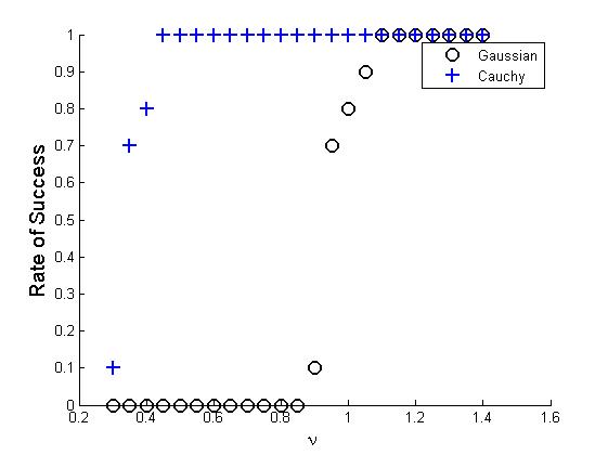
Figure 2: Support detection as a function of the separation constant $\nu$ for Cauchy and Gaussian kernels. For each value of $\nu$, 10 experiments were conducted with $\sigma=0.1$. An experiment is called a success if it detects the signal’s support precisely. Rate of success 1 means that the support was located precisely for all 10 experiments.

Figure 3 presents two examples for atomic decomposition of stream of Cauchy delays with $\sigma=0.1$ and $\nu=0.7$, contaminated with Gaussian noise (SNRs of $17.9$ and $27.5$ db). We mention that in order to achieve good recovery results we had to increase the separation constant. As can be seen, the solution in some cases misses the small delays of the signal, which are at the level of the noise, but manages to recover the larger delays with high accuracy.

$\begin{array}[]{cc}\includegraphics[scale={0.45}]{noisy_cauchy_20.jpg}&\includegraphics[scale={0.45}]{noisy_cauchy_60.jpg}\\ \mbox{(a)}&\mbox{(b)}\end{array}$

Figure 3: Atomic decomposition of stream of Cauchy delays with $\sigma=0.1$ and a separation constant of $\nu=0.7$ from noisy measurements with: (a) $\delta=20$ (SNR$=27.5$ db) (b) $\delta=60$ (SNR$=17.9$ db). The black line represents the noisy measurements, the blue circles represent the original signal, and the red asterisks the recovered signal.

5 Conclusions

In this paper, we have shown that a standard convex optimization technique can robustly decompose a stream of pulses into its atoms. The localization properties of the decomposition were derived in [5]. This holds provided that the distance between the atoms is of the order of $\sigma$ (see (1.1)), and that the kernel satisfies mild localization conditions. In contrast to previous works, our method is stable and relies on theoretical results on the continuum, implying that there is no limitation on the discretization step. In a consecutive paper [4], it was proven that the separation is unnecessary if the underlying signal is known to be positive (i.e. $c_{m}>0$). In this case, the separation can be replaced by a weaker condition of Rayleigh regularity.

Our results show that the minimal separation needed for the success of the recovery depends on the global and the local properties of the kernel. It seems that the degree of the kernel’s concavity near the origin has a particular importance, i.e. a ‘flat’ kernel near the origin requires higher separation.

We have showed explicitly that our technique applies to univariate and bivariate signals. We strongly believe that this result holds in higher dimensions since parts of the proof can be easily generalized to any dimension. However, there are certain technical challenges which we hope to overcome in future work.

This work is part of an ongoing effort to prove and demonstrate the effectiveness of convex optimization techniques to robustly recover signals from their projections onto polynomial spaces [13, 8, 6] and from their convolution with known kernels. The projection of signals onto spaces generated by shifts of one function or shifts and dilations of one function were investigated extensively in the literature [52, 17, 16, 33, 29, 14, 38, 11, 39, 49] and found many applications (see for instance [35, 27]). An interesting question is whether similar convex optimization techniques can be applied for the recovery of signals from these projections. We leave this question for a future research.

Acknowledgements

The authors thank Yonina Eldar and Gongguo Tang for helpful discussions and to the referees for valuable remarks.

References

• [1] J. Azais, Y. De Castro, and F. Gamboa. Spike detection from inaccurate samplings. Applied and Computational Harmonic Analysis, 38(2):177–195, 2015.
• [2] O. Bar-Ilan and Y.C. Eldar. Sub-nyquist radar via doppler focusing. IEEE Transactions on Signal Processing, 62(7):1796–1811, 2014.
• [3] A. Beck. Introduction to Nonlinear Optimization: Theory, Algorithms, and Applications with MATLAB, volume 19. SIAM, 2014.
• [4] T. Bendory. Robust recovery of positive stream of pulses. arXiv preprint arXiv:1503.08782, 2015.
• [5] T. Bendory, A. Bar-Zion, D. Adam, S. Dekel, and A. Feuer. Stable support recovery of stream of pulses with application to ultrasound imaging. To appear in IEEE Transactions on Signal Processing, 2016.
• [6] T. Bendory, S. Dekel, and A. Feuer. Exact recovery of non-uniform splines from the projection onto spaces of algebraic polynomials. Journal of Approximation Theory, 182(0):7 – 17, 2014.
• [7] T. Bendory, S. Dekel, and A. Feuer. Exact recovery of dirac ensembles from the projection onto spaces of spherical harmonics. Constructive Approximation, 42:183–207, 2015.
• [8] T. Bendory, S. Dekel, and A. Feuer. Super-resolution on the sphere using convex optimization. Signal Processing, IEEE Transactions on, 63(9):2253–2262, 2015.
• [9] T. Bendory and Y.C. Eldar. Recovery of sparse positive signals on the sphere from low resolution measurements. Signal Processing Letters, IEEE, 22(12):2383–2386, 2015.
• [10] B.N. Bhaskar, G. Tang, and B. Recht. Atomic norm denoising with applications to line spectral estimation. Signal Processing, IEEE Transactions on, 61(23):5987–5999, 2013.
• [11] M. Buhmann and A. Pinkus. Identifying linear combinations of ridge functions. Advances in Applied Mathematics, 22(1):103–118, 1999.
• [12] E.J. Candès and C. Fernandez-Granda. Super-resolution from noisy data. Journal of Fourier Analysis and Applications, 19(6):1229–1254, 2013.
• [13] E.J. Candès and C. Fernandez-Granda. Towards a mathematical theory of super-resolution. Communications on Pure and Applied Mathematics, 2013.
• [14] A. Cavaretta, W. Dahmen, and C. Micchelli. Stationary subdivision, volume 453. American Mathematical Soc., 1991.
• [15] Y. Chi, L.L. Scharf, A. Pezeshki, and A.R. Calderbank. Sensitivity to basis mismatch in compressed sensing. Signal Processing, IEEE Transactions on, 59(5):2182–2195, 2011.
• [16] C. De Boor, R.A. DeVore, and A. Ron. Approximation from shift-invariant subspaces of ${L}_{2}({R}^{d})$. Transactions of the American Mathematical Society, 341(2):787–806, 1994.
• [17] C. De Boor, R.A. DeVore, and A. Ron. The structure of finitely generated shift-invariant spaces in ${L}_{2}({R}^{d})$. Journal of Functional Analysis, 119(1):37–78, 1994.
• [18] Y. De Castro and F. Gamboa. Exact reconstruction using beurling minimal extrapolation. Journal of Mathematical Analysis and applications, 395(1):336–354, 2012.
• [19] Y. De Castro, F. Gamboa, D. Henrion, and J.B. Lasserre. Exact solutions to super resolution on semi-algebraic domains in higher dimensions. arXiv preprint arXiv:1502.02436, 2015.
• [20] Y. De Castro and G. Mijoule. Non-uniform spline recovery from small degree polynomial approximation. Journal of Mathematical Analysis and Applications, 2015.
• [21] D.L. Donoho. Compressed sensing. Information Theory, IEEE Transactions on, 52(4):1289–1306, 2006.
• [22] P.L. Dragotti, M. Vetterli, and T. Blu. Sampling moments and reconstructing signals of finite rate of innovation: Shannon meets strang–fix. Signal Processing, IEEE Transactions on, 55(5):1741–1757, 2007.
• [23] B. Dumitrescu. Positive trigonometric polynomials and signal processing applications. Springer, 2007.
• [24] V. Duval and G. Peyré. Exact support recovery for sparse spikes deconvolution. Foundations of Computational Mathematics, pages 1–41, 2015.
• [25] V. Duval and G. Peyré. Sparse spikes deconvolution on thin grids. arXiv preprint arXiv:1503.08577, 2015.
• [26] M. Elad. Sparse and redundant representations: from theory to applications in signal and image processing. Springer, 2010.
• [27] Y.C. Eldar. Sampling Theory: Beyond Bandlimited Systems. Cambridge University Press, 2015.
• [28] Carlos Fernandez-Granda. Super-resolution of point sources via convex programming. arXiv preprint arXiv:1507.07034, 2015.
• [29] V.I. Filippov and P. Oswald. Representation in lp by series of translates and dilates of one function. Journal of Approximation Theory, 82(1):15–29, 1995.
• [30] M. Grant and S. Boyd. CVX: Matlab software for disciplined convex programming, version 2.1, March 2014.
• [31] R.A. Horn and C.R. Johnson. Matrix analysis. 1985. Cambridge.
• [32] Y. Hua and T.K. Sarkar. Matrix pencil method for estimating parameters of exponentially damped/undamped sinusoids in noise. Acoustics, Speech and Signal Processing, IEEE Transactions on, 38(5):814–824, 1990.
• [33] R.Q. Jia and J. Wang. Stability and linear independence associated with wavelet decompositions. Proceedings of the American mathematical society, 117(4):1115–1124, 1993.
• [34] W. Liao and A. Fannjiang. Music for single-snapshot spectral estimation: Stability and super-resolution. Applied and Computational Harmonic Analysis, 2014.
• [35] S. Mallat. A wavelet tour of signal processing. Academic press, 1999.
• [36] K.V. Mishra, C. Myung, A. Kruger, and X. Weiyu. Spectral super-resolution with prior knowledge. Signal Processing, IEEE Transactions on, 63(20):5342–5357, 2015.
• [37] A. Moitra. The threshold for super-resolution via extremal functions. arXiv preprint arXiv:1408.1681, 2014.
• [38] I. Novikov, V. Protasov, and M. Skopina. Wavelet theory, volume 239. American Mathematical Soc., 2011.
• [39] A Pinkus. Smoothness and uniqueness in ridge function representation. Indagationes Mathematicae, 24(4):725–738, 2013.
• [40] R. Roy and T. Kailath. Esprit-estimation of signal parameters via rotational invariance techniques. Acoustics, Speech and Signal Processing, IEEE Transactions on, 37(7):984–995, 1989.
• [41] W. Rudin. Real and complex analysis (3rd). New York: McGraw-Hill Inc, 1986.
• [42] G. Schiebinger, E. Robeva, and B. Recht. Superresolution without separation. arXiv preprint arXiv:1506.03144, 2015.
• [43] R.O. Schmidt. Multiple emitter location and signal parameter estimation. Antennas and Propagation, IEEE Transactions on, 34(3):276–280, 1986.
• [44] P. Stoica and R.L Moses. Spectral analysis of signals. Pearson/Prentice Hall Upper Saddle River, NJ, 2005.
• [45] G. Tang, B.N. Bhaskar, and B. Recht. Sparse recovery over continuous dictionaries-just discretize. In Signals, Systems and Computers, 2013 Asilomar Conference on, pages 1043–1047, Nov 2013.
• [46] G. Tang, B.N. Bhaskar, and B. Recht. Near minimax line spectral estimation. Information Theory, IEEE Transactions on, 61(1):499–512, 2015.
• [47] G. Tang, B.N. Bhaskar, P. Shah, and B. Recht. Compressed sensing off the grid. Information Theory, IEEE Transactions on, 59(11):7465–7490, 2013.
• [48] G. Tang and B. Recht. Atomic decomposition of mixtures of translation-invariant signals. IEEE CAMSAP, 2013.
• [49] P.A Terekhin. Affine synthesis in the space ${L}_{2}({R}^{d})$. Izvestiya: Mathematics, 73(1):171, 2009.
• [50] R. Tur, Y.C. Eldar, and Z. Friedman. Innovation rate sampling of pulse streams with application to ultrasound imaging. Signal Processing, IEEE Transactions on, 59(4):1827–1842, 2011.
• [51] M. Vetterli, P. Marziliano, and T. Blu. Sampling signals with finite rate of innovation. Signal Processing, IEEE Transactions on, 50(6):1417–1428, 2002.
• [52] L.F. Villemoes. Wavelet analysis of refinement equations. SIAM Journal on Mathematical Analysis, 25(5):1433–1460, 1994.
• [53] N. Wagner, Y. C Eldar, and Z. Friedman. Compressed beamforming in ultrasound imaging. Signal Processing, IEEE Transactions on, 60(9):4643–4657, 2012.
• [54] F. Zhang. The Schur complement and its applications, volume 4. Springer Science & Business Media, 2006.