An empirical-parametric gamma calibration algorithm

Abstract

A method to determine the gamma correction curves for displays is presented. An empirical model is first constructed from exhaustive measurements of a few representative units. The model parameters for the remaining units are then fitted using only a few measurements. The method uses standard least-squares algorithms and is computationally light. Experimental results for a small sample of LCD displays are presented.

1 Introduction

Modern display devices generally incorporate a mechanism for adjustment of their gamma correction curves. This mechanism is used in the production line to correct for variations between units. In principle, the adjustment could be based on an exhaustive spectrographic measurement of each unit, but this would be time-consuming and expensive. In fast paced production lines, one needs to be able to adjust a device’s gamma curve with just a few spectrographic measurements.

One such approach is to fit or estimate a few parameters of a pre-defined mathematical model of the display, such as the LCD model of Kwak and MacDonald [3] or the CTR model of Berns [5]. This approach can provide good results if the model can accurately represent the device’s gamma curves with a small number of adjustable parameters. However, the gamma curves of a given production batch may have some peculiar characteristics that cannot easily be represented by a standard general-purpose model, and one then faces the problem of modifying the model to remove systemic deviations in the fitted curves. Existing mathematical models may also need to be modified when new display technologies or manufacturing methods are introduced.

In this work, we propose a gamma calibration method that combines the accuracy of exhaustive measurement with the efficiency of a parametric model. First, a parametric model is constructed from exhaustive measurements of a few representative units. Then, for each unit in the production line, the parameters of the model are fitted using only a few measurements. Because the method uses only standard least-squares algorithms, it is computationally light and reliable.

2 Preliminaries

In our setting the gamma response of a display unit is measured from grey levels. The unit is given an sRGB input with a grey color from white $(0,0,0)$ to black $(255,255,255)$, and the color that is displayed without any gamma correction is measured. The measurements are transformed to sRGB color space and scaled to the range $(0,0,0)-(255,255,255)$.

The actual gamma correction is generally applied to each RGB channel separately, thus we will study the channels separately, and the resulting algorithm is to be applied to each channel accordingly. The separation of color channels and the assumption of channel independence is a usual characteristic of display control systems, as mentioned by Kazuhiro [2].

Now, we have $J$ display units measured thoroughly with responses $d_{i,j}$, where subindex $i$ indicates the measured grey level and $j$ the display unit. We call these $J$ units the training sample. The measurements are done on $I$ different grey levels $x_{i}\in(0...255)$.

For the unit that we are to calibrate, we have $P$ responses $d^{\prime}_{p}$ at grey levels $x_{i_{p}}$, where we have $P\leq J$ and $p\in[1...P]$, $i_{p}\in I$, where $I$ is an index set with the indices of the measured colors. Our goal is to estimate the responses at other grey levels (the gamma correction curve) accurately even when $P$ is small.

3 The method

Let $A$ be the $J$-by-$256$ matrix of the training set responses of a color channel, say the red channel. An element $a_{i,j}$ of $A$ is the response to input $(j-1)$th input grey level of the $i$th display.

We estimate the response of this color channel of the test unit one grey level at a time, as follows. Suppose we are estimating the response for input level $x$. We first extract the columns of $A$ that correspond to the measured values and the columns that correspond to the input level value we are to estimate. Thus we get a $J$-by-$(P+1)$ matrix $A_{x}$. For convenience we put values corresponding to $x$ in the first column.

The rows of $A_{x}$ are now treated as samples from $(P+1)$-dimensional normal distribution with mean $\mu$ and covariance $\Sigma$. Both $\mu$ and $\Sigma$ can be estimated from the rows of $A_{x}$ by standard techniques.

Consider now the measurements we have from the test unit. We have $P$ measured values and one unknown. We arrange these to a vector $(x,\vec{y})$ where $\vec{y}$ models the measured values and $x$ is unknown. Notice that the order of elements of $(x,\vec{y})$ naturally follows that of the matrix $A_{x}$. The vector $(x,\vec{y})$ can now be thought of as a sample from the distribution $\operatorname{\mathcal{N}}_{x}(\mu,\Sigma)$ and we would like to estimate how $x$ is distributed when we know the value of $\vec{y}$.

Since the value of $\vec{y}$ is known we can estimate the distribution of $x$ with a conditional distribution. The conditional distribution of one of the dimensions is constructed as follows. First we partition $\mu$ as

$$\mu=\blockarray{ccc}&{\scriptstyle 1}{\scriptstyle P}\\ \block{c(cc)}{\scriptstyle 1}\mu_{1}\mu_{2}\\$$

and $\Sigma$ as

$$\Sigma=\blockarray{ccc}{\scriptstyle 1}&{\scriptstyle P}\,\\ \block{(cc)c}\Sigma_{11}\Sigma_{12}\,\,\,\,{\scriptstyle 1}\\ \Sigma_{21}\Sigma_{22}\,\,\,\,{\scriptstyle P}\\$$ (1)

We are now to find the conditional distribution of $x$ given $\vec{y}=a$, i.e. $(x\mid\vec{y}=a)$, where $a$ contains the values measured from the display for which we want the estimate. The conditional distribution of $(x\mid\vec{y}=a)$ is $\operatorname{\mathcal{N}}(\mu^{\prime},\Sigma^{\prime})$ where

$$\mu^{\prime}=\mu_{1}+\Sigma_{12}\Sigma_{22}^{-1}(a-\mu_{2})$$

and

$$\Sigma^{\prime}=\Sigma_{11}-\Sigma_{12}\Sigma_{22}^{-1}\Sigma_{21}.$$

Here the matrix $\Sigma_{22}^{-1}$ is generalized inverse, also known Moore-Penrose inverse, of $\Sigma_{22}$, see [4] for further details. Now the predicted value for $x$ is $\mu^{\prime}$ and $\Sigma^{\prime}$ provides us confidence intervals if wanted.

This algorithms computes the pseudoinverse $\Sigma_{22}^{-1}$ via singular value decomposition because it provides good numerical stability. For further information see for example Golub & Loan [1].

4 Experiments

We tested the method with a sample of ten displays. The displays in the sample were measured on black $(0,0,0)$ and grey values $(1,1,1)$, $(3,3,3)$,…, $(255,255,255)$ totaling to $129$ measured grey levels. The results for red channel are shown in Figure 1. We notice the slightly clustered nature of the displays and one display that variates from the others. The used scaling guarantees us that on $(0,0,0)$ and $(255,255,255)$ all responses are equal.

We treated nine of the displays as a training sample and predicted the response values for the remaining unit. The tests were run on red channel.

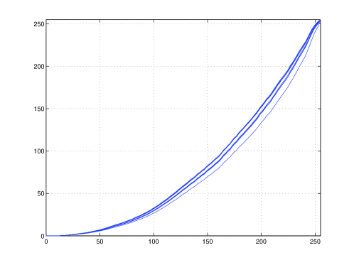
Figure 1: Responses of training sample of red channel.

We tested the algorithm with one, two and three measured grey levels, thus $P$ is $1$, $2$, and $3$ respectively. The tests were run on various displays and the results are practically uniform across the data. The results for the chosen test unit on red channel are in Figure 2. Notice that the error escalates slightly when we drop the number of measurements to two and even more when only one value is used on the prediction. It is readily seen that with only three grey levels we reach quite satisfying prediction. One should notice that four grey levels would make the fit worse in the test case because we have only nine displays in the training sample, which makes the estimate of the covariance matrix problematic.

For the test unit the prediction error is of the same magnitude for each color channel. Figure 3 shows the prediction errors for each color channel when three grey levels were measured: $(117,117,117)$, $(177,177,177)$ and $(217,217,127)$. Unfortunately there is no established method for choosing the grey levels. The values were first chosen to be almost equispaced and later finetuned to the chosen values. The differences between tested values were not big.

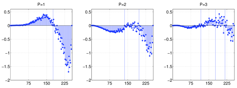
Figure 2: The error in red color channel with one, two and three measured grey levels. Vertical lines indicate the measured valued.

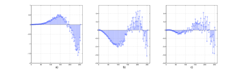
Figure 3: Error in prediction for the unit by color channel.

5 Conclusions

We used the assumption that the data is normal distributed. Figure 1 does, however, suggest that a suitable bimodal distribution might provide better results. In any case, the data set is relatively small and not much can be inferred about the (assumed) underlying distribution.

Also, a larger training sample would provide more freedom on choosing the number of measurements. Now the number of measurements we can use is limited by the amount of data, because estimating the covariance matrix becomes problematic. In theory one could overcome the situation with a least-square fit but in our tests the least-square solution proved to introduce big errors on bright values.

References

- [1] G.H. Golub and C.F Van Loan, ”Matrix Computations” (Johns Hopkins Studies in the Mathematical Sciences, 1996).
- [2] Kazuhiro Sato, ”Image-Processing Algorithms” (Image Sensors and Signal Processing for Digital Still Cameras, Edited by Junichi Nakamura, CRC Press, 2005)
- [3] Y. Kwak and L. MacDonald, ”Characterisation of a desktop LCD projector ”, Displays 21(5), 179 - 194 (2000)
- [4] J.W. Demmel, ”Applied Numerical Linear Algebra”, (Society for Industrial and Applied Mathematics, 1997)
- [5] R. S. Berns, ”Methods for characterizing CRT displays ”, Displays 16(4), 173 - 182 (1996),