Enhancement and reduction of one-dimensional heat conduction with correlated mass disorder

Abstract

Short-range order in strongly disordered structures plays an important role in their heat conduction property. Using numerical and analytical methods, we show that short-range spatial correlation (with a correlation length of $\Lambda_{m}$) in the mass distribution of the one-dimensional (1D) alloy-like random binary lattice leads to a dramatic enhancement of the high-frequency phonon transmittance but also increases the low-frequency phonon opacity. High-frequency semi-extended states are formed while low-frequency modes become more localized. This results in ballistic heat conduction at finite lengths but also paradoxically higher thermal resistance that scale as $\sqrt{\Lambda_{m}}$ in the $L\rightarrow\infty$ limit. We identify an emergent crossover length ($L_{c}$) below which the onset of thermal transparency appears. The crossover length is linearly dependent on but is two orders of magnitude larger than $\Lambda_{m}$. Our results suggest that the phonon transmittance spectrum and heat conduction in a disordered 1D lattice can be controlled via statistical clustering of the constituent component atoms into domains. They also imply that the detection of ballistic heat conduction in disordered 1D structures may be a signature of the intrinsic mass correlation at a much smaller length scale.

I Introduction

Phonon-mediated heat conduction in low-dimensional nanostructures is a transport phenomenon of fundamental and applied interest. Maldovan (2013) In particular, the manipulation of the thermal conductivity in nanomaterials may enable the realization of potential applications in thermoelectric devices, solid state refrigeration and thermal cloaking. Han et al. (2013) One approach is to use a low-dimensional material such as nanowires Zou and Balandin (2001); Li et al. (2003a); Hochbaum et al. (2008); Nika et al. (2013) in which confinement alters the intrinsic phononic properties (e.g., anisotropy, dispersion and mean free path). The other is to use a bulk material such as Si or Ge and modify its thermal conductivity ($\kappa$) via nanostructuring. This includes the creation of periodic patterns (e.g., Si-Ge superlattices Simkin and Mahan (2000); Li et al. (2003b); Dames and Chen (2004); Chen et al. (2013) and nanopore arrays Hopkins et al. (2011); Yu et al. (2010); Jain et al. (2013)), the use of resonant superstructures Davis and Hussein (2014), and alloying. Zhu et al. (2009) The latter appears to be one of the more promising options for obtaining the reduced thermal conductivity needed for efficient and cost-effective thermoelectric devices because an abrupt decrease in $\kappa$ can be observed upon the introduction of a small alloy concentration. Zhu et al. (2009) Alloying can also be combined with confinement to further reduce the thermal conductivity.

The low thermal conductivity in alloys can be attributed in part to mode localization which stems from the random placement of the component atoms and impedes phonon propagation. For the finite three-dimensional disordered harmonic solid, it has been shown that only delocalized modes contribute significantly to the heat current. Allen and Feldman (1993); Feldman et al. (1993) In one dimension (1D) in particular, disorder results in the localization of all the modes in in the thermodynamic ($L\rightarrow\infty$) limit Matsuda and Ishii (1970); Ishii (1973); Dhar (2001) although for a finite system, a fraction of the states would always be sufficiently extended to contribute to the heat current. Dhar (2008) Valuable insights into the interplay between localization and propagation in 1D can be gleaned within the framework of the disordered harmonic chain (DHC), the simplest model of a disordered 1D structure that has been frequently used to understand the effect of disorder on heat conduction. Rubin (1968); Dhar (2001); Ong and Zhang (2014) Broadly speaking, we know that disorder leads to the exponential attenuation of the phonon transmittance $\Xi$, i.e., $\Xi(\omega,L)\sim\exp[-L/\lambda(\omega)]$, where $\omega$ and $\lambda$ are the frequency and attenuation length, respectively, in analogy to the Beer-Lambert law in optics, Ong and Zhang (2014) and is a direct consequence of localization. Matsuda and Ishii (1970); Ishii (1973); Dhar (2001) It follows from the known $\lambda\propto\omega^{-2}$ relationship Ong and Zhang (2014) that the thermal conductivity scales as $\lim_{L\rightarrow\infty}\kappa\propto L^{0.5}$ and $\lim_{L\rightarrow\infty}\kappa\propto\langle\delta m\rangle^{-1}$, where $L$ and $\langle\delta m\rangle$ are respectively the length and mass fluctuation, for free boundary conditions. Matsuda and Ishii (1970); Visscher (1971); Rubin and Greer (1971); Greer and Rubin (1972); Lepri et al. (2003).

On the other hand, these semirigorous results have only been established for the case of heat conduction with purely random (uncorrelated) mass disorder, in which the position of the mass fluctuation is uncorrelated across different atomic sites. Rubin (1968); Matsuda and Ishii (1970); Ishii (1973); Dhar (2001) In an alloy, this disorder manifests itself as the uncorrelated placement of the constituent atoms. However, when there is statistical clustering of the atoms in the form of domains, the position of the atoms and the spatial distribution of mass become correlated, introducing short-range order and modifying the localization phenomenon. A considerable amount of work has been done by de Moura and co-workers de Moura et al. (2003, 2006) who showed by using numerical simulations that long-range correlation leads to the formation of low-energy extended states in the DHC. Duda and co-workers have also studied the effects of atomic ordering on the thermal conductivity by using molecular dynamics simulations. Duda et al. (2011, 2012) Using an analytical approach, Herrera-Gonzalez and co-workers Herrera-Gonzalez et al. (2010) also studied the relationship between the scaling of the thermal conductivity with system size and long-range correlated isotopic disorder. They demonstrate that specific long-range correlations can suppress or enhance the heat current contribution of vibrational modes in pre-defined frequency windows. However, their results are confined to the case of weak isotopic disorder and weak coupling between the lattice and the heat baths, owing to the nature of their perturbative approximations. Their numerical simulations are also limited to systems with $N\leq 10^{3}$, where $N$ is the number of atoms. Here, we adopt a numerical approach in this paper to more fully and systematically explore the implications of short-range correlated mass disorder for heat conduction, especially with regard to its dependence on length ($N\leq 1.6\times 10^{5}$) and the extent of the short-range order in mass correlation.

In this paper, we report the effect of short-range mass correlation (or correlated disorder, for short) on phonon transmittance and heat conduction through a random binary lattice (RBL), an alloy-like realization of the DHC. We restrict ourselves to the coherent processes and neglect anharmonic effects from inelastic scattering between phonons. This allows us to isolate the effects of disorder on heat conduction in micrometer-scale systems, and we expect our results to be applicable to 1D alloy nanostructures for which the reduced thermal conductivity can be traced to mass disorder. Larkin and McGaughey (2013); Hori et al. (2013) In the following sections, we first describe the 1D lattice model and how correlated disorder is generated for the lattice. The short-range order in the mass correlation, in the form of an exponentially decaying spatial correlation, is characterized by a correlation length of $\Lambda_{m}$. Next, the phonon transmittance is calculated for the uncorrelated and correlated model. We find from numerical simulations that the short-range correlation in the mass distribution, through the formation of domains, leads to an emergent crossover length scale ($L_{c}$) below which the system is effectively transparent over a wide phonon frequency range and conducts heat ballistically. At very low frequencies, mass correlation decreases the attenuation length while at higher frequencies, the attenuation length actually increases. Thus, when $L$ exceeds $L_{c}$, one sees a rapid onset of phononic opacity, resulting in a dramatic increase in the thermal resistance exceeding that in the DHC with uncorrelated mass disorder. More intriguingly, $L_{c}$ is two orders of magnitude larger than $\Lambda_{m}$. We find a formula that connects the mass correlation length and the increase in thermal resistance in long chains. Finally, we discuss the connection between our purely 1D results to heat conduction in more realistic systems, and how correlated mass disorder can affect heat conduction at length scales much larger than the correlation length. We also interpret the recent findings of ballistic heat conduction in SiGe-alloy nanowires in Ref. Hsiao et al. (2013) in light of our results.

II Methodology

II.1 Random binary lattice model

We choose as our model system the familiar disordered harmonic chain first studied by Dyson, Dyson (1953) which we also used in our earlier paper. Ong and Zhang (2014) Our system differs from that used in other papers in that the atomic mass is not treated as a continuous random variable. de Moura et al. (2003); Bodyfelt et al. (2013) Rather, we have a random binary lattice, where the positions of the component atoms are set probabilistically so that the lattice resembles more realistic alloy systems with mass disorder. For simplicity, only adjacent atoms are coupled. The atoms are only permitted to move longitudinally and no attempt is made to include any anharmonic interaction in our model.

Our system consists of three parts. In the middle, there is a finite-size “conductor” of $N$ equally spaced atoms. On either side, there is a homogeneous lead, i.e., a semi-infinite chain with no mass disorder. In effect, we have a finite disordered system embedded in an infinite homogeneous 1D lattice, which also corresponds to a finite disordered harmonic chain with free boundaries. Rubin and Greer (1971); Dhar (2001) The homogeneous leads act as heat reservoirs and are coupled to the conductor via the same harmonic spring terms as those between the atoms in the disordered lattice. Coupling between adjacent atoms is governed by the harmonic spring term $V(x_{i},x_{i+1})=\frac{1}{2}k(x_{i}-x_{i+1})^{2}$ where $k$ is the spring constant and $x_{i}$ is the displacement of the $i$-th atom from its equilibrium position. In the RBL, there are two species of atoms which we label A and B. Species A is taken to be the substitutional impurity and exists only within the conductor. The rest of the atoms in the conductor and the leads are of species B. We set the mass of the A (B) atoms to $m_{A}=9.2\times 10^{-26}$ kg ($m_{B}=4.6\times 10^{-26}$ kg, the mass of a Si atom), the spring constant to $k=32$ Nm^-1 (the approximate strength of the Si-Si bond) and the interatomic spacing to $a=0.55$ nm. Our choice of parameters follows that in Ref. Zhang et al. (2007). The maximum simulated chain length is $N=1.6\times 10^{5}$ or $L=Na=88$ $\mu$m.

II.2 Short-range order in lattice

We define the mass fluctuation correlation function as $\left\langle\delta m(x)\delta m(x^{\prime})\right\rangle=\left\langle m(x)m(x^{\prime})\right\rangle-\left\langle m(x)\right\rangle^{2}$, where $m(x)$ is the atomic mass at site $x$. It measures the short-range correlation in mass fluctuation (or mass correlation for short). In RBL, we set the distribution of the constituent atoms such that the mass correlation has the exponential form

$$\left\langle\delta m(x)\delta m(x^{\prime})\right\rangle=c_{A}c_{B}\Delta m^{2}\exp(-|x-x^{\prime}|/\Lambda_{m})\ ,$$ (1)

where $\Delta m=|m_{A}-m_{B}|$ and $c_{A}$ ($c_{B}$) is the concentration of A (B) atoms. For pure random disorder ($\Lambda_{m}=0$), the mass correlation function is $\left\langle\delta m(x)\delta m(0)\right\rangle=c_{A}c_{B}(m_{A}-m_{B})^{2}\delta_{x,0}$. To generate the lattice configuration with the mass correlation in Eq. (1), we first divide the conductor into smaller domains alternating between having all A or all B atoms. The number of sites in each domain of A atoms ($d_{A}$) is generated according to the probability distribution $P(d)=\langle d_{A}\rangle^{-1}\exp(-d/\langle d_{A}\rangle)$ where $\langle d_{A}\rangle=\Lambda_{m}[a(1-c_{A})]^{-1}$ is the average type-A domain size. The size of each type-B domain ($d_{B}$) is similarly defined. For simplicity’s sake, we set $c_{A}=c_{B}=0.5$. In the uncorrelated disorder case, we do not create smaller domains but instead set the probability of each site having an A (B) atom to $c_{A}$ ($c_{B}$). Figure 1 shows the normalized mass correlation function $\left\langle\delta m(x)\delta m(x^{\prime})\right\rangle/\left\langle\delta m(x)^{2}\right\rangle$ for uncorrelated and correlated ($\Lambda_{m}=10a$) mass disorder. A schematic representation of the mass distribution can also be seen in the inset of Fig. 1.

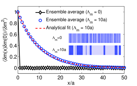
Figure 1: (Color online) Plot of the ensemble-average mass correlation function for uncorrelated (diamond symbol, $\Lambda_{m}=0$) and correlated (circle symbol, $\Lambda_{m}=10a$) mass disorder at $c_{A}=c_{B}=0.5$. The mass correlation is calculated numerically from 100 realizations of disorder. The analytical fit based on Eq. (1) is also shown (dashed line). A representative schematic of their mass distributions is shown in the inset. The correlated distribution consists of much larger domains of A and B atoms.

II.3 Phonon transmittance calculation

There are two approaches to computing the phonon transmittance through the RBL. The first is the well-known nonequilibrium Green’s function method Zhang et al. (2007); Mingo (2009) in which the transmittance is given by $\Xi(\omega)=\text{Tr}(\boldsymbol{\Gamma_{L}G\Gamma_{R}G^{\dagger}})$, where $G$ is the nonequilibrium Green’s function and $\Gamma_{L}$ ($\Gamma_{R}$) is the term coupling the left (right) lead to the conductor. More details of this method can be found in Refs. Zhang et al. (2007); Ong and Zhang (2014). The second approach is via the eigenvalue of the products of transfer matrices, de Moura et al. (2003, 2006) which we describe in Appendix A. In either case, the ensemble average of the transmittance $\langle\Xi(\omega)\rangle$ is taken over 100 independent realizations of mass disorder.

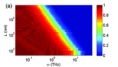
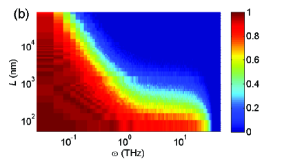
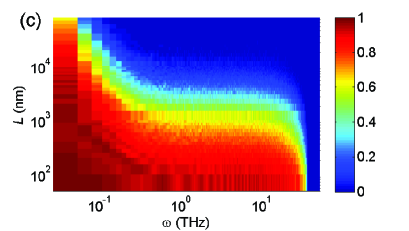
Figure 2: (Color online) Plot of transmittance function $\langle\Xi(\omega,L)\rangle$ as a function of chain length $L$ and frequency $\omega$ for (a) $\Lambda_{m}=0$, (b) $\Lambda_{m}=10a$, and (c) $\Lambda_{m}=50a$. In the uncorrelated case ($\Lambda_{m}=0$), the transmittance scales as $\langle\Xi(\omega,L)\rangle\sim\exp[-L/\lambda(\omega)]$ where $\lambda\propto\omega^{-2}$. However, for the correlated mass distribution in (b) and (c), the transmittance has the form $\langle\Xi(\omega,L)\rangle\sim\exp[-L/\lambda(\omega)]$ but the attenuation length no longer scales as $\lambda\propto\omega^{-2}$. In the intermediate frequency range ($\omega=$1-10 THz) for $\Lambda_{m}=50a$, the attenuation length is almost a constant with $\lambda\sim 3$ $\mu$m or about two orders of magnitude larger than $\Lambda_{m}$.

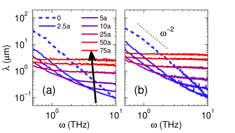
Figure 3: (Color online) Plot of the attenuation length $\lambda$ computed from (a) the transfer matrix method and (b) the transmittance function, as a function of frequency $\omega$ for different values of the mass correlation length ($\Lambda_{m}/a=0$, 2.5, 5, 10, 25, 50 and 75) in the frequency range of 0.5 to 10 THz. The attenuation length in (a) is slightly smaller than in (b). However, the change in $\lambda$ with $\Lambda_{m}$ is qualitatively the same for both methods. The arrow indicates the direction of increasing $\Lambda_{m}$. In the uncorrelated case ($\Lambda_{m}=0$), the attenuation length scales as $\lambda\propto\omega^{-2}$. Mass correlation increases (decreases) the attenuation length at high (low) frequencies. In the 0.5 to 10 THz range, the attenuation length for $\Lambda_{m}=75a$ (or 41.25 nm) is around 3 $\mu$m, about 2 orders of magnitude larger. We interpret this as the formation of semi-extended vibrational states.

III Results

III.1 Length dependence of phonon transmittance

Figure 2 shows the transmittance as a function of $L$ and $\omega$ for (a) $\Lambda_{m}=0$, (b) $\Lambda_{m}=10a$, and (c) $\Lambda_{m}=50a$. In the uncorrelated case in Fig. 2(a), the transmittance function scales as $\langle\Xi(\omega,L)\rangle=\exp\left[-L/\lambda(\omega)\right]$, where $\lambda\propto\omega^{-2}$. In Fig. 2(b), when $\Lambda_{m}=10a$, the attenuation length still scales as $\lambda\propto\omega^{-2}$ at low frequencies but for $\omega>1$ THz, it deviates from that behavior as it varies weakly with $\omega$ at a characteristic length scale of $\lambda\sim$ 0.5 $\mu$m. Figure 2(c) also shows a frequency regime in which $\lambda$ is weakly $\omega$ dependent in the range 0.5 to 10 THz. The characteristic attenuation length scale is, however, at $\sim 2.5$ $\mu$m. The plots in Fig. 2 show that a finite $\Lambda_{m}$ alters the attenuation length at high frequencies. To see this more clearly, we plot $\lambda(\omega)$ in Fig. 3 estimated numerically from (a) the Lyapunov exponent [$\lambda=a(2\gamma)^{-1}$] and (b) the attenuation of the transmittance function [$\lambda(\omega)=\int dL\ \langle\Xi(\omega,L)\rangle$]. There is good agreement between the $\lambda(\omega)$ values computed from the two methods with the $\lambda$ from (b) being slightly larger.

Two trends are immediately clear in Fig. 3. Firstly, a nonzero $\Lambda_{m}$ causes the attenuation length to deviate from $\lambda_{0}$ ($\Lambda_{m}=0$). At higher frequencies, transmittance is enhanced, i.e., $\lambda>\lambda_{0}$. As $\Lambda_{m}$ increases, the frequency range in which $\lambda$ is weakly $\omega$-dependent becomes wider. Furthermore, $\lambda\gg\Lambda_{m}$, and $\lambda(\omega)$ also increases with $\Lambda_{m}$. Secondly, transmittance is reduced at low frequencies, i.e., $\lambda<\lambda_{0}$. The low-frequency phononic opacity is increased by the mass correlation. The weak $\omega$ dependence of the attenuation length of the higher-frequency modes also implies that these modes are ‘semi-extended’ and participate in ballistic heat conduction when the lattice size is comparable to their attenuation lengths. Physically, the short-range order in the mass distribution results in the partial delocalization of the higher-frequency modes but greater localization of the low-frequency modes. This alters the relative participation of the phonon modes in length-dependent heat conduction.

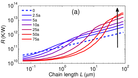
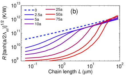
Figure 4: (Color online) (a) Plot of the thermal resistance $R$ as a function of chain length $L$ for for different values of the mass correlation length ($\Lambda_{m}/a=0$, 2.5, 5, 10, 25, 50 and 75) in the $T\rightarrow\infty$ limit. The arrow indicates the direction of increasing $\Lambda_{m}$. For $\Lambda_{m}=0$, i.e., the uncorrelated case, $R$ scales as $R\propto L^{0.5}$, as expected. However, when mass correlation is finite, the thermal resistance relative to the uncorrelated case decreases at small $L$. As $L\rightarrow 0$, the resistance converges to a constant, implying the existence of ballistic heat conduction. At large $L$, the thermal resistance goes up as we increase the mass correlation length. (b) Plot of the rescaled thermal resistance normalized by $[\tanh(\frac{a}{2\Lambda_{m}})]^{1/2}$ as a function of $L$. In the $L\rightarrow\infty$ limit, $R[\tanh(\frac{a}{2\Lambda_{m}})]^{1/2}$ for different values of $\Lambda_{m}$ appears to converge.

III.2 Thermal resistance

To determine the effect of the altered transmittance on heat conduction, we compute the length-dependent thermal resistance $R(L)$ using the Landauer formula: Zhang et al. (2007); Mingo (2009)

$$R(L)=\left[\frac{1}{2\pi}\int_{0}^{\omega_{L}}\hbar\omega\frac{df(\omega)}{dT}\langle\Xi(\omega,L)\rangle\ d\omega\right]^{-1}$$ (2)

where $T$ and $\hbar$ are respectively the temperature and Planck constant, and $f(\omega)=[\exp(\frac{\hbar\omega}{k_{B}T})-1]^{-1}$is the Bose-Einstein occupation factor. $\omega_{L}$ is the cutoff frequency determined by the pristine lead ($\omega_{L}=\sqrt{4k/m_{B}}$). $\langle\Xi(\omega,L)\rangle$ is derived from our nonequilibrium Green’s function (NEGF) computation. In the high-temperature limit, Eq. (2) becomes $\lim_{T\rightarrow\infty}R(L)=\left[\frac{k_{B}}{2\pi}\int_{0}^{\infty}\langle\Xi(\omega,L)\rangle\ d\omega\right]^{-1}$.

The high-temperature thermal resistance is shown in Fig. 4(a) for different values of $\Lambda_{m}$ ($\Lambda_{m}/a=0$, 2.5, 5, 10, 25, 50 and 75). We take the $\Lambda_{m}=0$ curve (which we term $R_{0}$) to be the baseline for comparison. $R_{0}(L)$ scales as $L^{0.5}$ at all values of $L$, as predicted for uncorrelated disorder. However, for correlated disorder ($\Lambda_{m}\neq 0$), $R(L)$ deviates from the $R\propto L^{0.5}$ behavior. At small $L$, $R<R_{0}$ and is weakly dependent on $L$, implying that the system conducts heat ballistically. This is due to the enhanced attenuation length and transmittance of the high-frequency modes relative to the uncorrelated case. We also observe that $\lim_{L\rightarrow 0}R$ converges to the same value ($R=\frac{\sqrt{8}\pi}{k_{B}\omega_{L}}\approx 1.2\times 10^{10}$K/W) regardless of the correlation length. This value is determined by the cutoff frequency and impurity mass. As $L\rightarrow\infty$, the relative contribution of the low-frequency modes grows. Thus, $R$ increases rapidly and exceeds $R_{0}$, scaling as $L^{0.5}$, because of greater low-frequency phononic opacity.

We quantify the dependence of the thermal resistance on mass correlation here in the $L\rightarrow\infty$ limit. As noted earlier, the ratio $\lim_{L\rightarrow\infty}R/R_{0}$ grows monotonically with $\Lambda_{m}$. The thermal resistance in the $\Lambda_{m}=0$ case, Ong and Zhang (2014)

$$\lim_{L\rightarrow\infty}R_{0}(L)=\sqrt{\frac{4\pi\langle\delta m^{2}\rangle L}{ka\langle m\rangle k_{B}^{2}}}\ ,$$ (3)

is proportional to the local mass fluctuation $\sqrt{\langle\delta m^{2}\rangle}$. Equation (3) is generalized (see Appendix B for the derivation) by replacing $\langle\delta m^{2}\rangle$ with $\sum_{x}\langle\delta m(x)\delta m(0)\rangle$, which sums over the mass fluctuation across atomic sites, to yield

$$\lim_{L\rightarrow\infty}R(\Lambda_{m},L)=\sqrt{\frac{4\pi\sum_{x}\langle\delta m(x)\delta m(0)\rangle L}{ka\langle m\rangle k_{B}^{2}}}$$ (4)

where $\langle\delta m(x)\delta m(0)\rangle=\langle\delta m^{2}\rangle e^{-|x|/\Lambda_{m}}$, giving us $\lim_{L\rightarrow\infty}R(\Lambda_{m},L)=R_{0}(L)[\tanh(\frac{a}{2\Lambda_{m}})]^{-1/2}$ since $\lim_{N\rightarrow\infty}\sum_{x=-Na}^{Na}e^{-|x|/\Lambda_{m}}=1/\tanh(\frac{a}{2\Lambda_{m}})$. We recover Eq. (3) from Eq. (4) for $\Lambda_{m}=0$, while for large $\Lambda_{m}$, we obtain $\lim_{L\rightarrow\infty}R(\Lambda_{m},L)\propto\sqrt{\Lambda_{m}}$. It should be noted that the results in Eqs. (3) and (4) are derived assuming that the semi-infinite homogeneous leads act as heat baths and are coupled to the lattice via the same harmonic spring terms as those between the atoms in the disordered lattice. We plot the normalized thermal resistance $R[\tanh(\frac{a}{2\Lambda_{m}})]^{1/2}$ in Fig. 4(b). In the $L\rightarrow\infty$ limit, $R[\tanh(\frac{a}{2\Lambda_{m}})]^{1/2}$ for different values of $\Lambda_{m}$ converges to $R_{0}(L)$, suggesting that Eq. (4) captures the effect of mass correlation on thermal resistance.

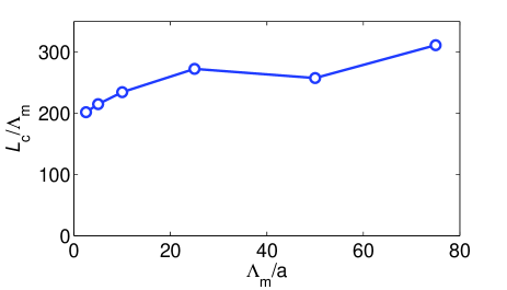
Figure 5: (Color online) Plot of the ratio of the crossover length $L_{c}$ to the mass correlation length $\Lambda_{m}$ as a function of $\Lambda_{m}$. The crossover length is the minimum attenuation length at which $\lambda(\Lambda_{m},\omega)>\tanh(\frac{a}{2\Lambda_{m}})\lambda(\Lambda_{m}=0,\omega)$, i.e., $\lambda$ deviates from the $\lambda\propto\omega^{-2}$ behavior. We observe that $L_{c}$ is about 250 times (or two orders of magnitude) larger than $\Lambda_{m}$.

III.3 Crossover length

At low frequency, the attenuation length for the uncorrelated case is $\lim_{\omega\rightarrow 0^{+}}\lambda_{0}(\omega)=4ka\langle m\rangle/(\langle\delta m^{2}\rangle\omega^{2})$. Ong and Zhang (2014) The corresponding attenuation length for correlated disorder is $\lim_{\omega\rightarrow 0^{+}}\lambda(\Lambda_{m},\omega)=\tanh(\frac{a}{2\Lambda_{m}})\lambda(\Lambda_{m}=0,\omega)$ (see Appendix A for the derivation). In the $\Lambda_{m}\rightarrow 0$ limit, we recover $\lim_{\omega\rightarrow 0^{+},\Lambda_{m}\rightarrow 0}\lambda(\Lambda_{m},\omega)=\lambda_{0}(\omega)$ while for large $\Lambda_{m}$, we obtain $\lim_{\omega\rightarrow 0^{+}}\lambda(\Lambda_{m},\omega)\propto 1/\Lambda_{m}$, i.e., the attenuation length is inversely proportional to the mass correlation length.

We define the crossover length scale $L_{c}$ as the minimum attenuation length at which $\lambda(\Lambda_{m},\omega)\geq\tanh(\frac{a}{2\Lambda_{m}})\lambda(\Lambda_{m}=0,\omega)$, i.e., the smallest attenuation length for the correlated case is greater than or equal to the rescaled attenuation length for the uncorrelated length. Physically, $L_{c}$ sets the length scale above which Eq. (4) describes the thermal resistance and the $R\propto L^{-0.5}$ scaling behavior applies as the contribution of the semi-extended high-frequency modes vanishes. For $L\ll L_{c}$, the system becomes thermally transparent [i.e., $\langle\Xi(\omega,L)\rangle\approx 1$] and heat conduction becomes quasiballistic given the participation of the semi-extended states. Figure 5 shows the numerically computed ratio $L_{c}/\Lambda_{m}$ as a function of $\Lambda_{m}$. We observe that $L_{c}$ averages about 250 times (or two orders of magnitude) larger than $\Lambda_{m}$ over the range of correlation lengths considered. This demonstrates that ballistic heat conduction over a given length may be associated with a mass correlation that is two orders of magnitude smaller.

IV Discussion

Our simulation results imply that heat conduction in alloys is not merely a function of the mass difference and the relative concentrations Ong and Zhang (2014) but also depends on the mass distribution. In the perfect alloy, the solubility of the component species is assumed to be equal and the atoms are randomly distributed across lattice sites. However, differences in miscibility  and growth kinetics Yu et al. (1996) may lead to phase segregation or the formation of domains, Aqua et al. (2013) introducing short-range order in the mass distribution and forming semi-extended high-frequency modes that are spatially larger than the correlation length. Hence, it is possible for an alloy 1D nanostructure to conduct heat ballistically at a finite length scale that is much larger than the average domain size. The key point here is that the short-range order drastically increases the localization length of these high-frequency modes, allowing them to contribute substantially to heat conduction. Furthermore, the weakly frequency-dependent localization length of the high-frequency modes sets an intrinsic length scale below which a change in the length of the lattice does not affect the phonon contribution to the heat current, i.e., the coherent heat conduction can be ballistic over a finite length.

The interplay between ordering and heat conduction has been observed in planar SiGe superlattices. Chen et al. (2013) Chen and co-workers found that the thermal conductivity is considerably lower in SiGe with pure layers separated by sharp interfaces than it is in homogeneous SiGe alloys. This is attributed to the higher scattering efficiency of low-frequency phonons by the pure domains created from the long-range compositional order. Moreover, the thermal conductivity is further reduced when there is some grading in the concentration profile at the interface which introduces short-range disorder and enhances the scattering of higher-frequency phonons. This variation in the thermal conductivity and frequency-dependent scattering efficiency in the superlattice structure highlights the role of correlated disorder in heat conduction.

To elucidate the effect of correlated disorder in quasi-one-dimensional nanostructures, we calculate the thermal resistance as a function of length for a model 1.1 nm-wide rectangular Si nanowire that has a 50:50 mix of isotopes at 300 K. To mimic the effect of mass disorder in a Si_0.5Ge_0.5 nanowire, we set the atomic mass of the lighter and heavier isotope to be equal to that of Si and Ge, respectively. The transmittance is calculated using the NEGF method and then used to compute the thermal resistance [see Eq. (2)] as a function of temperature. Figure 6 shows the results averaged over ten instances of disorder for uncorrelated and correlated ($\Lambda_{m}=20a$ or 11 nm) disorder for nanowires up to 2.5 $\mu$m. We observe that the thermal resistance in the uncorrelated case is significantly more length dependent than in the correlated case where the weak length dependence suggests ballistic heat conduction and is reminiscent of the experimental results observed in Ref. Hsiao et al. (2013). Qualitatively, the length dependence is also similar to that in Fig. 4(a) where a finite correlation length also leads to micrometer-scale quasiballistic heat conduction. While our model represents a very drastic idealization of real SiGe nanowires with anharmonic phonon-phonon interactions and boundary scattering completely neglected, it does suggest that even some short-range order can have a dramatic effect on heat conduction in quasi-one-dimensional nanostructures, especially when phonon transport is limited by alloy scattering.

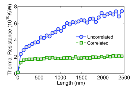
Figure 6: (Color online) Thermal resistance as a function of length for a strongly mass-disordered 1.1 nm-wide rectangular Si nanowire with uncorrelated (circle) and correlated (square) disorder. Fifty percent of the atoms have their masses set equal to that of Ge while the rest have theirs set to that of Si. The correlation length in the correlated disorder case is 11 nm.

Our results also highlight the role of short-range order in the alloy structure on phonon-mediated heat conduction, a factor which has not been given significant consideration in the literature. It is known that the attenuation length $\lambda$ in the transmittance is proportional to the mean free path via the Thouless relation. Anderson et al. (1980); Savić et al. (2008) Thus, if the positions of the alloy atoms are correlated, our results imply that the mean free paths of the low-frequency phonons are accordingly reduced while those of the high-frequency modes are extended, modifying the phonon contribution balance to the thermal conductivity. One potential application of this is the manipulation of the thermal conductivity of alloys by controlling the spatial distribution of the alloy components. One approach to the control of heat flow has been to engineer the spectrum of the phonons in order to select for phonons of specific frequencies that can be managed by a periodic structure. Maldovan (2013) In particular, the fabrication of thermocrystals Maldovan (2013) requires the suppression of the very-low-frequency phonons which may be realized by using a SiGe alloy with finite short-range order.

V Conclusion

We have simulated heat conduction in the 1D alloy-like RBL for correlated and uncorrelated mass disorder. We find that correlated mass disorder enhances (reduces) the high-frequency (low-frequency) phonon transmittance, leading to ballistic heat conduction that persists over a length scale that is two orders of magnitude larger than the mass correlation length. However, in very large systems, correlated mass disorder increases the thermal resistance of the system because of the greater low-frequency phononic opacity.

Appendix A Analytical estimate of low-frequency inverse localization length for correlated mass disorder

We derive an analytical expression for the inverse localization length in the $\omega\rightarrow 0^{+}$ limit for a given mass correlation, using the transfer matrix method. Derrida et al. (1987); Kissel (1991) The transmittance through a lattice of $N$ atoms can be written as the absolute square of the transmission function, i.e., $\Xi(\omega)=|\tau_{N}|^{2}$, where $\tau_{N}$ is the transmission function with the amplitude $\lim_{N\rightarrow\infty}|\tau_{N}|=\exp[-\gamma(\omega)N]$. The inverse localization length $\gamma$ (also commonly known as the Lyapunov exponent) at frequency $\omega$ is thus defined as

$$\gamma(\omega)=\lim_{N\rightarrow\infty}\frac{1}{N}\ln|\tau_{N}|\ ,$$ (5)

and $|\tau_{N}|$ can be computed from the norm of the product of $N$ transfer matrices Dhar (2001), i.e.,

$$|\tau_{N}|=\left\|\prod_{p=1}^{N}T_{p}\right\|\ .$$ (6)

The transmittance attenuation length is $\lambda(\omega)=a[2\gamma(\omega)]^{-1}$, where $a$ is the interatomic spacing. $\lambda$ can be directly computed numerically from Eqs. (5) and (6), as in Refs. de Moura et al. (2003, 2006), or estimated analytically in the $\omega\rightarrow 0$ limit as follows.

The $p$-th transfer matrix in Eq. (6) is defined as

$$T_{p}=\left(\begin{array}[]{cc}2-x_{p}&-1\\ 1&0\end{array}\right)\ ,$$ (7)

where $x_{p}$ is the dimensionless random variable corresponding to the $p$-th atom in the chain such that $x_{p}=m_{p}\omega^{2}/k$ and $0\leq x_{p}\leq 2$, and is a particular formulation of the equation of motion for the spatial displacement of the $p$-th atom. de Moura et al. (2003)

For weak disorder or at low frequencies, we can find an analytical approximation for the localization length following the method described in Refs. Derrida et al. (1987); Kissel (1991). Let $x_{p}=\langle x\rangle+\delta x_{p}$ where $\langle x_{p}\rangle=\langle x\rangle$ and $\langle\delta x_{p}\rangle=0$. The expression in Eq. (7) can thus be linearized as

$$T_{p}=\left(\begin{array}[]{cc}2-\langle x\rangle&-1\\ 1&0\end{array}\right)+\left(\begin{array}[]{cc}-1&0\\ 0&0\end{array}\right)\delta x_{p}\ .$$

We choose an eigenvector transformation $U$, such that $\tilde{T}_{p}=U^{\dagger}T_{p}U$, to obtain

$$\tilde{T}_{p}=\left(\begin{array}[]{cc}e^{i\theta}&0\\ 0&e^{-i\theta}\end{array}\right)+\frac{1}{2i\sin\theta}\left(\begin{array}[]{cc}-e^{i\theta}&-e^{-i\theta}\\ e^{i\theta}&e^{-i\theta}\end{array}\right)\delta x_{p}$$

where $\theta$ is defined by $\cos\theta=1-\frac{1}{2}\langle x\rangle$ and $\sin\theta=[\langle x\rangle-\langle x\rangle^{2}/4]^{1/2}$. For notational convenience, we define

$$A=\left(\begin{array}[]{cc}e^{i\theta}&0\\ 0&e^{-i\theta}\end{array}\right)$$

$$B=\frac{1}{2i\sin\theta}\left(\begin{array}[]{cc}-e^{i\theta}&-e^{-i\theta}\\ e^{i\theta}&e^{-i\theta}\end{array}\right)$$

so that we can write the $p$-th transfer matrix as $\tilde{T}_{p}=A+B\delta x_{p}$. The $N$-product of the transfer matrices is

$$\prod_{p=1}^{N}\tilde{T}_{p}=(A+B\delta x_{1})\ldots(A+B\delta x_{N})\ .$$ (8)

The expression in Eq. (8) can be systematically expanded in powers of $\delta x_{p}$. The zeroth-, first- and second-order terms are

$$A^{N}\ ,$$ (9)

$$\sum_{p=1}^{N}A^{p-1}BA^{N-p}\delta x_{p}$$ (10)

and

$$\sum_{p=1}^{N-1}\sum_{q=p+1}^{N}A^{p-1}BA^{q-p-1}BA^{N-q}\delta x_{p}\delta x_{q}\ ,$$ (11)

respectively. To find the low-frequency scaling behavior, we need only consider the zeroth- and first-order terms. Thus, we write Eq. (8) as

$$\prod_{p=1}^{N}\tilde{T}_{p}\approx A^{N}+\sum_{p=1}^{N}A^{p-1}BA^{N-p}\delta x_{p}\ .$$ (12)

The (1,1) term of the $2\times 2$ matrix in Eq. (12) is equal to $1/\tau_{N}$, and after some algebra, can be written as $e^{iN\theta}[1-(2i\sin\theta)^{-1}\sum_{p=1}^{N}\delta x_{p}]$. Hence,

$$|\tau_{N}|^{2}=\left[1+i\frac{\cos N\theta}{\sin\theta}\sum_{p=1}^{N}\delta x_{p}+\frac{1}{4\sin^{2}\theta}\left(\sum_{p=1}^{N}\delta x_{p}\right)^{2}\right]^{-1}$$

and its logarithm can be approximated as

$$\ln|\tau_{N}|^{2}\approx-\frac{i\cos N\theta}{\sin\theta}\sum_{p=1}^{N}\delta x_{p}-\frac{1}{4\sin^{2}\theta}\left(\sum_{p=1}^{N}\delta x_{p}\right)^{2}\ .$$ (13)

The localization length is defined as $\gamma=-\lim_{N\rightarrow\infty}\frac{1}{N}\langle\ln|\tau_{N}|\rangle$. The ensemble averaging $\langle\ldots\rangle$ removes the terms linear in $\delta x_{n}$ in Eq. (13). Bearing in mind that we are only considering the low-frequency scaling behavior, the expression for the inverse localization length is

$$\lim_{\omega\rightarrow 0^{+}}\gamma(\omega) = \lim_{N\rightarrow\infty}\frac{1}{8N\sin^{2}\theta}\left\langle\left(\sum_{p=1}^{N}\delta x_{p}\right)^{2}\right\rangle$$ (14)

$$= \lim_{N\rightarrow\infty}\frac{1}{8N\sin^{2}\theta}\sum_{p=1}^{N}\sum_{q=1}^{N}\langle\delta x_{p}\delta x_{q}\rangle\ .$$

In the correlated case,

$$\langle\delta x_{p}\delta x_{q}\rangle=\langle\delta x^{2}\rangle\exp(-|x_{p}-x_{q}|/\Lambda_{m})$$

and the double sum in Eq. (14) becomes

$$\sum_{p=1}^{N}\sum_{q=1}^{N}\langle\delta x_{p}\delta x_{q}\rangle\approx N\langle\delta x^{2}\rangle\coth\left(\frac{a}{2\Lambda_{m}}\right)\ .$$

Therefore, the inverse localization length is

$$\lim_{\omega\rightarrow 0^{+}}\gamma(\omega)\approx\frac{\langle\delta m^{2}\rangle\omega^{2}}{8k\langle m\rangle}\coth\left(\frac{a}{2\Lambda_{m}}\right)\ .$$ (15)

Note that in the uncorrelated case, the correlation length is $\Lambda_{m}=0$ and the expression in Eq. (15) yields

$$\lim_{\omega\rightarrow 0^{+}}\gamma(\omega)=\frac{\langle\delta m^{2}\rangle\omega^{2}}{8k\langle m\rangle}$$

as expected. We remind the reader that the analytical expression in Eq. (15) only applies at low frequencies. At higher frequencies, this approximation fails and the Lyapunov exponent is calculated directly from Eq. (5).

Appendix B Thermal resistance in the thermodynamic ($L\rightarrow\infty$) limit for correlated mass disorder

Given the expression for $\gamma(\omega)$ in Eq. (15), we can obtain the expression for the thermal resistance in the $L\rightarrow\infty$ limit. The phonon transmittance is

$$\lim_{L\rightarrow\infty}\langle\Xi(\omega,L)\rangle=\exp[-2\gamma(\omega)L/a]$$

and the high-temperature length-dependent thermal conductance is

$$\lim_{L\rightarrow\infty}\sigma(L)=\frac{k_{B}}{2\pi}\int_{0}^{\infty}\langle\Xi(\omega,L)\rangle\ d\omega\ .$$ (16)

The integrand in Eq. (16) vanishes as $\omega\rightarrow\infty$ and only its low-frequency part contributes to the integral, allowing us to use Eq. (15). Thus, the explicit expression for Eq. (16) is

$$\lim_{L\rightarrow\infty}\sigma(L)=\left[\frac{ka\langle m\rangle k_{B}^{2}}{4\pi\langle\delta m\rangle^{2}L}\tanh\left(\frac{a}{2\Lambda_{m}}\right)\right]^{1/2}\ .$$

As a function of the mass correlation length, the asymptotic ($L\rightarrow\infty$) expression for the thermal resistance $R=1/\sigma$ is

$$\lim_{L\rightarrow\infty}R(\Lambda_{m},L)=\frac{R_{0}(L)}{\sqrt{\tanh\left(\frac{a}{2\Lambda_{m}}\right)}}$$

where $R_{0}(L)=\lim_{L\rightarrow\infty}R(\Lambda_{m}=0,L)\ .$

References

- Maldovan (2013) M. Maldovan, Phys. Rev. Lett. 110, 025902 (2013).
- Han et al. (2013) T. Han, T. Yuan, B. Li, and C.-W. Qiu, Sci. Rep. 3, 1593 (2013).
- Zou and Balandin (2001) J. Zou and A. Balandin, J. Appl. Phys. 89, 2932 (2001).
- Li et al. (2003a) D. Li, Y. Wu, P. Kim, L. Shi, P. Yang, and A. Majumdar, Appl. Phys. Lett. 83, 2934 (2003a).
- Hochbaum et al. (2008) A. I. Hochbaum, R. Chen, R. D. Delgado, W. Liang, E. C. Garnett, M. Najarian, A. Majumdar, and P. Yang, Nature 451, 163 (2008).
- Nika et al. (2013) D. L. Nika, A. I. Cocemasov, D. V. Crismari, and A. A. Balandin, Appl. Phys. Lett. 102, 213109 (2013).
- Simkin and Mahan (2000) M. V. Simkin and G. D. Mahan, Phys. Rev. Lett. 84, 927 (2000).
- Li et al. (2003b) D. Li, Y. Wu, R. Fan, P. Yang, and A. Majumdar, Appl. Phys. Lett. 83, 3186 (2003b).
- Dames and Chen (2004) C. Dames and G. Chen, J. Appl. Phys. 95, 682 (2004).
- Chen et al. (2013) P. Chen, N. A. Katcho, J. P. Feser, W. Li, M. Glaser, O. G. Schmidt, D. G. Cahill, N. Mingo, and A. Rastelli, Phys. Rev. Lett. 111, 115901 (2013).
- Hopkins et al. (2011) P. E. Hopkins, C. M. Reinke, M. F. Su, R. H. Olsson III, E. A. Shaner, Z. C. Leseman, J. R. Serrano, L. M. Phinney, and I. El-Kady, Nano Lett. 11, 107 (2011).
- Yu et al. (2010) J.-K. Yu, S. Mitrovic, D. Tham, J. Varghese, and J. R. Heath, Nature Nanotech. 5, 718 (2010).
- Jain et al. (2013) A. Jain, Y.-J. Yu, and A. J. H. McGaughey, Phys. Rev. B 87, 195301 (2013).
- Davis and Hussein (2014) B. L. Davis and M. I. Hussein, Phys. Rev. Lett. 112, 055505 (2014).
- Zhu et al. (2009) G. H. Zhu, H. Lee, Y. C. Lan, X. W. Wang, G. Joshi, D. Z. Wang, J. Yang, D. Vashaee, H. Guilbert, A. Pillitteri, M. S. Dresselhaus, G. Chen, and Z. F. Ren, Phys. Rev. Lett. 102, 196803 (2009).
- Allen and Feldman (1993) P. B. Allen and J. L. Feldman, Phys. Rev. B 48, 12581 (1993).
- Feldman et al. (1993) J. L. Feldman, M. D. Kluge, P. B. Allen, and F. Wooten, Phys. Rev. B 48, 12589 (1993).
- Matsuda and Ishii (1970) H. Matsuda and K. Ishii, Suppl. Prog. Theor. Phys. 45, 56 (1970).
- Ishii (1973) K. Ishii, Suppl. Prog. Theor. Phys. 53, 77 (1973).
- Dhar (2001) A. Dhar, Phys. Rev. Lett. 86, 5882 (2001).
- Dhar (2008) A. Dhar, Adv. Phys. 57, 457 (2008).
- Rubin (1968) R. J. Rubin, J. Math. Phys. 9, 2252 (1968).
- Ong and Zhang (2014) Z.-Y. Ong and G. Zhang, J. Phys.: Condens. Matter 26, 335402 (2014).
- Visscher (1971) W. M. Visscher, Prog. Theor. Phys. 46, 729 (1971).
- Rubin and Greer (1971) R. J. Rubin and W. L. Greer, J. Math. Phys. 12, 1686 (1971).
- Greer and Rubin (1972) W. L. Greer and R. J. Rubin, J. Math. Phys. 13, 379 (1972).
- Lepri et al. (2003) S. Lepri, R. Livi, and A. Politi, Physics Reports 377, 1 (2003).
- de Moura et al. (2003) F. A. B. F. de Moura, M. D. Coutinho-Filho, E. P. Raposo, and M. L. Lyra, Phys. Rev. B 68, 012202 (2003).
- de Moura et al. (2006) F. A. B. F. de Moura, L. P. Viana, and A. C. Frery, Phys. Rev. B 73, 212302 (2006).
- Duda et al. (2011) J. C. Duda, T. S. English, D. A. Jordan, P. M. Norris, and W. A. Soffa, J. Phys. Condens. Matter 23, 205401 (2011).
- Duda et al. (2012) J. C. Duda, T. S. English, D. A. Jordan, P. M. Norris, and W. A. Soffa, J. Heat Transfer 134, 014501 (2012).
- Herrera-Gonzalez et al. (2010) I. F. Herrera-Gonzalez, F. M. Izrailev, and L. Tessieri, Europhys. Lett. 90, 14001 (2010).
- Larkin and McGaughey (2013) J. M. Larkin and A. J. H. McGaughey, J. Appl. Phys. 114, 023507 (2013).
- Hori et al. (2013) T. Hori, T. Shiga, and J. Shiomi, J. Appl. Phys. 113, 203514 (2013).
- Hsiao et al. (2013) T.-K. Hsiao, H.-K. Chang, S.-C. Liou, M.-W. Chu, S.-C. Lee, and C.-W. Chang, Nature Nanotech. 8, 534 (2013).
- Dyson (1953) F. J. Dyson, Phys. Rev. 92, 1331 (1953).
- Bodyfelt et al. (2013) J. D. Bodyfelt, M. C. Zheng, R. Fleischmann, and T. Kottos, Phys. Rev. E 87, 020101 (2013).
- Zhang et al. (2007) W. Zhang, T. Fisher, and N. Mingo, Numerical Heat Transfer, Part B: Fundamentals 51, 333 (2007).
- Mingo (2009) N. Mingo, in Thermal Nanosystems and Nanomaterials (Springer, 2009) pp. 63–94.
- Yu et al. (1996) Q. Yu, M. O. Thompson, and P. Clancy, Phys. Rev. B 53, 8386 (1996).
- Aqua et al. (2013) J.-N. Aqua, I. Berbezier, L. Favre, T. Frisch, and A. Ronda, Physics Reports 522, 59 (2013).
- Anderson et al. (1980) P. W. Anderson, D. J. Thouless, E. Abrahams, and D. S. Fisher, Phys. Rev. B 22, 3519 (1980).
- Savić et al. (2008) I. Savić, N. Mingo, and D. A. Stewart, Phys. Rev. Lett. 101, 165502 (2008).
- Derrida et al. (1987) B. Derrida, K. Mecheri, and J. Pichard, Journal de Physique 48, 733 (1987).
- Kissel (1991) G. J. Kissel, Phys. Rev. A 44, 1008 (1991).