Secular dynamics of hierarchical quadruple systems: the case of a triple system orbited by a fourth body

Adrian S. Hamers1, Hagai B. Perets2, Fabio Antonini3 and Simon F. Portegies Zwart1
1Leiden Observatory, Leiden University, PO Box 9513, NL-2300 RA Leiden, The Netherlands
2Technion - Israel Institute of Technology, Haifa 32000, Israel
3Center for Interdisciplinary Exploration and Research in Astrophysics (CIERA), and Department of Physics and Astronomy, Northwestern University,
2145 Sheridan Road, Evanston, IL 60208, USA
E-mail: hamers@strw.leidenuniv.nl
(MNRAS 449, 1, 4221-4245 (2015)
Accepted 2015 February 27. Received 2014 February 25; in original form 2014 December 5)
Abstract

We study the secular gravitational dynamics of quadruple systems consisting of a hierarchical triple system orbited by a fourth body. These systems can be decomposed into three binary systems with increasing semimajor axes, binaries A, B and C. The Hamiltonian of the system is expanded in ratios of the three binary separations, and orbit averaged. Subsequently, we numerically solve the equations of motion. We study highly hierarchical systems that are well described by the lowest order terms in the Hamiltonian. We find that the qualitative behaviour is determined by the ratio 0subscript0\mathcal{R}_{0} of the initial Kozai-Lidov (KL) time-scales of the binary pairs AB and BC. If 01much-less-thansubscript01\mathcal{R}_{0}\ll 1, binaries AB remain coplanar if this is initially the case, and KL eccentricity oscillations in binary B are efficiently quenched. If 01much-greater-thansubscript01\mathcal{R}_{0}\gg 1, binaries AB become inclined, even if initially coplanar. However, there are no induced KL eccentricity oscillations in binary A. Lastly, if 01similar-tosubscript01\mathcal{R}_{0}\sim 1, complex KL eccentricity oscillations can occur in binary A that are coupled with the KL eccentricity oscillations in B. Even if binaries A and B are initially coplanar, the induced inclination can result in very high eccentricity oscillations in binary A. These extreme eccentricities could have significant implications for strong interactions such as tidal interactions, gravitational wave dissipation, and collisions and mergers of stars and compact objects. As an example, we apply our results to a planet+moon system orbiting a central star, which in turn is orbited by a distant and inclined stellar companion or planet, and to observed stellar quadruples.

keywords:
gravitation – celestial mechanics – planet-star interactions – stars: kinematics and dynamics.
pubyear: 2015pagerange: Secular dynamics of hierarchical quadruple systems: the case of a triple system orbited by a fourth body16

1 Introduction

Hierarchical triple systems are known to be common among stellar systems. For example, a fraction of 0.076 of FG dwarfs systems in the catalogue of Tokovinin (2014a, b) are triple systems (in the fractions cited here from Tokovinin 2014b, completeness arguments have been taken into account; the observed number of triple systems in the sample of Tokovinin 2014a is 290, with a total number of 4847 systems). The triple fraction is likely higher for more massive stars. In such hierarchical systems, the torque of the outer binary can induce high-amplitude oscillations in the inner binary over time-scales that can vary from suborbital time-scales, to time-scales exceeding Gyr. These oscillations, known as Kozai-Lidov (KL) cycles (Lidov, 1962; Kozai, 1962), have important implications for a large range of astrophysical systems, in particular when the effects of tidal friction are also considered. The implications include the production of short-period binaries and hot Jupiters (Eggleton & Kiseleva-Eggleton, 2001; Wu & Murray, 2003; Eggleton & Kisseleva-Eggleton, 2006; Fabrycky & Tremaine, 2007; Wu et al., 2007; Correia et al., 2011; Naoz et al., 2011; Naoz et al., 2012; Petrovich, 2014), accelerating the merging of compact objects (Blaes et al., 2002; Thompson, 2011; Antonini & Perets, 2012; Antonini et al., 2014), explaining some of the blue stragglers stars (Perets & Fabrycky, 2009; Naoz & Fabrycky, 2014), affecting the formation of binary minor planets (Perets & Naoz, 2009), possibly producing a special type of type Ia supernovae through collisions of white dwarfs (Katz & Dong, 2012; Hamers et al., 2013; Prodan et al., 2013), and modifying the evolution of stellar binaries that would not interact in the absence of a third star (Hamers et al., 2013).

Nature does not stop at N=3𝑁3N=3, however. Although in the catalogue of Tokovinin (2014a, b) triple systems, with a fraction of 0.580.580.58 (observed: 290 of 350), are most common among systems with hierarchies (N3𝑁3N\geq 3), quadruple systems also constitute a considerable fraction of hierarchical systems, i.e. a fraction of 0.320.320.32 (observed: 55 of 350). Unlike hierarchical triple systems, for which only one dynamically stable configuration is known to exist in nature, there are two different hierarchical configurations for which quadruples are known to be dynamically stable. One of these consists of two binary systems that orbit each other’s barycentre, and this type of system constitutes a fraction of 0.740.740.74 (observed: 37 of 55) of the quadruple systems in the catalogue of Tokovinin (2014a, b). The long-term dynamical evolution of this configuration has been studied by Pejcha et al. (2013), who showed, by means of direct N𝑁N-body simulations, that eccentricity oscillations, in particular orbital flips, can be enhanced in these systems relative to triples.

The other configuration consists of a hierarchical triple system that is orbited by a fourth body (referred to as a 3+1 quadruple system in Tokovinin 2014b), and is the focus of this paper. In this case, three binary systems can be identified, and we will assume that they are each sufficiently separated from each other such that the quadruple system is dynamically stable. A stability analysis of these systems is beyond the scope of this work. Here, we shall always assume stability, although stability of some systems is borne out by our direct N𝑁N-body integrations. We will refer to the binaries with the smallest, intermediate, and largest semimajor axes, as ‘binary A’, ‘binary B’ and ‘binary C’, respectively. A schematic depiction of our configuration is shown in Fig. 1.

Our hierarchical configuration not only applies to stellar quadruples, but also arises in other astrophysical systems. These include, but are not limited to, multiplanet, planet-moon and binary asteroid systems in single and binary star systems. Here, we study the case of a planet+moon system (binary A) that orbits a star (binary B), which in turn is orbited by a more distant and inclined object (binary C), e.g. another planet or star. We assume that the orbit of the planet+moon system is initially coplanar with respect to that of the primary star. Therefore, in the absence of a distant body, no excitation of the eccentricity of the orbit of the planet+moon system is expected. However, we will show that, in the presence of an inclined fourth body, high-amplitude eccentricity oscillations can be induced in the planet+moon system through an intricate coupling of KL cycles.

The structure of this paper is as follows. In Section 2, we describe our methods. We expand the four-body Hamiltonian in terms of the separation ratios rA/rBsubscript𝑟Asubscript𝑟Br_{\mathrm{A}}/r_{\mathrm{B}}, rB/rCsubscript𝑟Bsubscript𝑟Cr_{\mathrm{B}}/r_{\mathrm{C}} and rA/rCsubscript𝑟Asubscript𝑟Cr_{\mathrm{A}}/r_{\mathrm{C}}. In order for our method to be suitable for the study of the long-term evolution of a large number of systems, we adopt the secular approximation, i.e. we average the Hamiltonian over the three binary orbits assuming unperturbed and bound orbits for time-scales shorter than the orbital periods. Subsequently, we numerically solve the equations of motion derived from the orbit-averaged Hamiltonian. We test our method by comparing to direct N𝑁N-body integrations. In Section 3, we consider the general dynamics of highly hierarchical systems, i.e. systems that are well-described by the lowest-order terms in the Hamiltonian. We discuss our results in Section 4 and apply them to planetary and stellar systems. We give our conclusions in Section 5.

Refer to caption
Figure 1: A schematic depiction of the hierarchical configuration of the quadruple systems considered in this paper.

2 Methods

2.1 Expansion of the Hamiltonian

Our method to study the long-term evolution of quadruple systems is a natural extension to the orbit-averaged techniques that have been used extensively in the past to study the evolution of hierarchical triple systems, where an expansion was made in terms of the semimajor axis ratio ain/aoutsubscript𝑎insubscript𝑎outa_{\mathrm{in}}/a_{\mathrm{out}}, with ainsubscript𝑎ina_{\mathrm{in}} and aoutsubscript𝑎outa_{\mathrm{out}} the semimajor axes of the inner and outer orbit, respectively (Lidov, 1962; Kozai, 1962; Harrington, 1968, 1969; Ford et al., 2000; Eggleton & Kiseleva-Eggleton, 2001; Laskar & Boué, 2010; Naoz et al., 2013a). We note that hierarchical systems with more complex configurations have also been studied using secular methods by Touma et al. (2009) and Boué & Fabrycky (2014). We expand the Hamiltonian in terms of the separation ratios rA/rBsubscript𝑟Asubscript𝑟Br_{\mathrm{A}}/r_{\mathrm{B}}, rB/rCsubscript𝑟Bsubscript𝑟Cr_{\mathrm{B}}/r_{\mathrm{C}} and rA/rCsubscript𝑟Asubscript𝑟Cr_{\mathrm{A}}/r_{\mathrm{C}}, where the separation vectors 𝒓Asubscript𝒓A\boldsymbol{r}_{\mathrm{A}}, 𝒓Bsubscript𝒓B\boldsymbol{r}_{\mathrm{B}} and 𝒓Csubscript𝒓C\boldsymbol{r}_{\mathrm{C}} are defined in terms of the position vectors of the four bodies in equation (25). By assumption, rCrBrAmuch-greater-thansubscript𝑟Csubscript𝑟Bmuch-greater-thansubscript𝑟Ar_{\mathrm{C}}\gg r_{\mathrm{B}}\gg r_{\mathrm{A}}; therefore, these ratios are small and such an expansion is appropriate. The expansion is carried out to up and including fourth order in the separation ratios, i.e. including terms proportional to (rA/rB)i(rB/rC)j(rA/rC)ksuperscriptsubscript𝑟Asubscript𝑟B𝑖superscriptsubscript𝑟Bsubscript𝑟C𝑗superscriptsubscript𝑟Asubscript𝑟C𝑘(r_{\mathrm{A}}/r_{\mathrm{B}})^{i}(r_{\mathrm{B}}/r_{\mathrm{C}})^{j}(r_{\mathrm{A}}/r_{\mathrm{C}})^{k}, where 0i+j+k40𝑖𝑗𝑘40\leq i+j+k\leq 4. The details are given in Appendix A.1. For completeness, in addition to the configuration of a triple system orbited by a fourth body that is the focus of this paper, we have included results for the configuration of two binaries orbiting each other’s barycentre in Appendix A.2.

As derived in Appendix A.1, at the lowest order, i+j+k=1𝑖𝑗𝑘1i+j+k=1, the Hamiltonian consists of three terms that reduce to the binary binding energies of the three binaries A, B and C, assuming Kepler orbits. These terms therefore do not lead to secular orbital changes. At the next order, the ‘quadrupole’ order (i+j+k=2𝑖𝑗𝑘2i+j+k=2)111The term ‘quadrupole’ is not to be confused with ‘quadruple’., we find three terms, each of which is mathematically equivalent to the quadrupole-order Hamiltonian in the three-body problem. These three terms can also be obtained from the three-body quadrupole order Hamiltonian by appropriate substitutions of the masses and separation vectors.

More specifically, the (non-averaged) three-body Hamiltonian at the quadrupole order is given by

Hquad=Gm1m2m3m1+m21rout(rinrout)212[3(𝒓^in𝒓^out)21],subscript𝐻quad𝐺subscript𝑚1subscript𝑚2subscript𝑚3subscript𝑚1subscript𝑚21subscript𝑟outsuperscriptsubscript𝑟insubscript𝑟out212delimited-[]3superscriptsubscript^𝒓insubscript^𝒓out21\displaystyle H_{\mathrm{quad}}=-\frac{Gm_{1}m_{2}m_{3}}{m_{1}+m_{2}}\frac{1}{r_{\mathrm{out}}}\left(\frac{r_{\mathrm{in}}}{r_{\mathrm{out}}}\right)^{2}\frac{1}{2}\left[3\left(\hat{\boldsymbol{r}}_{\mathrm{in}}\cdot\hat{\boldsymbol{r}}_{\mathrm{out}}\right)^{2}-1\right], (1)

where 𝒓insubscript𝒓in\boldsymbol{r}_{\mathrm{in}} and 𝒓outsubscript𝒓out\boldsymbol{r}_{\mathrm{out}} are the separation vectors of the inner and outer binary, respectively. In our four-body system, the Hamiltonian, to the corresponding level of approximation, is given by three terms. These are each obtained from equation (1) by the following substitutions of separation vectors,

  1. 1.

    𝒓in𝒓Asubscript𝒓insubscript𝒓A\boldsymbol{r}_{\mathrm{in}}\rightarrow\boldsymbol{r}_{\mathrm{A}} and 𝒓out𝒓Bsubscript𝒓outsubscript𝒓B\boldsymbol{r}_{\mathrm{out}}\rightarrow\boldsymbol{r}_{\mathrm{B}} (AB);

  2. 2.

    𝒓in𝒓Bsubscript𝒓insubscript𝒓B\boldsymbol{r}_{\mathrm{in}}\rightarrow\boldsymbol{r}_{\mathrm{B}} and 𝒓out𝒓Csubscript𝒓outsubscript𝒓C\boldsymbol{r}_{\mathrm{out}}\rightarrow\boldsymbol{r}_{\mathrm{C}} (BC);

  3. 3.

    𝒓in𝒓Asubscript𝒓insubscript𝒓A\boldsymbol{r}_{\mathrm{in}}\rightarrow\boldsymbol{r}_{\mathrm{A}} and 𝒓out𝒓Csubscript𝒓outsubscript𝒓C\boldsymbol{r}_{\mathrm{out}}\rightarrow\boldsymbol{r}_{\mathrm{C}} (AC),

and masses

  1. 1.

    (no substitutions) (AB);

  2. 2.

    m1m1+m2subscript𝑚1subscript𝑚1subscript𝑚2m_{1}\rightarrow m_{1}+m_{2}, m2m3subscript𝑚2subscript𝑚3m_{2}\rightarrow m_{3} and m3m4subscript𝑚3subscript𝑚4m_{3}\rightarrow m_{4} (BC);

  3. 3.

    m3m4subscript𝑚3subscript𝑚4m_{3}\rightarrow m_{4} (AC).

In the quadrupole-order approximation, there are no terms appearing in the Hamiltonian that depend on all three position vectors 𝒓Asubscript𝒓A\boldsymbol{r}_{\mathrm{A}}, 𝒓Bsubscript𝒓B\boldsymbol{r}_{\mathrm{B}} and 𝒓Csubscript𝒓C\boldsymbol{r}_{\mathrm{C}}. This is no longer the case for the next order, the ‘octupole’ order (i+j+k=3𝑖𝑗𝑘3i+j+k=3). For the latter order, we find three terms that correspond to the octupole order terms in the three-body problem, and that can be obtained directly from the substitutions given above. In addition, we find a term that is a function of 𝒓Asubscript𝒓A\boldsymbol{r}_{\mathrm{A}}, 𝒓Bsubscript𝒓B\boldsymbol{r}_{\mathrm{B}} and 𝒓Csubscript𝒓C\boldsymbol{r}_{\mathrm{C}}. We will refer to such terms as ‘cross terms’. The cross term at octupole order is given by

Hoct,cross=Gm1m2m3m4(m1+m2)(m1+m2+m3)1rC(rArC)2(rBrC)subscript𝐻octcross𝐺subscript𝑚1subscript𝑚2subscript𝑚3subscript𝑚4subscript𝑚1subscript𝑚2subscript𝑚1subscript𝑚2subscript𝑚31subscript𝑟Csuperscriptsubscript𝑟Asubscript𝑟C2subscript𝑟Bsubscript𝑟C\displaystyle H_{\mathrm{oct,\,cross}}=\frac{Gm_{1}m_{2}m_{3}m_{4}}{(m_{1}+m_{2})(m_{1}+m_{2}+m_{3})}\frac{1}{r_{\mathrm{C}}}\left(\frac{r_{\mathrm{A}}}{r_{\mathrm{C}}}\right)^{2}\left(\frac{r_{\mathrm{B}}}{r_{\mathrm{C}}}\right)
×12[15(𝒓^B𝒓^C)(𝒓^A𝒓^C)23(𝒓^B𝒓^C)\displaystyle\quad\times\frac{1}{2}\left[15\left(\hat{\boldsymbol{r}}_{\mathrm{B}}\cdot\hat{\boldsymbol{r}}_{\mathrm{C}}\right)\left(\hat{\boldsymbol{r}}_{\mathrm{A}}\cdot\hat{\boldsymbol{r}}_{\mathrm{C}}\right)^{2}-3\left(\hat{\boldsymbol{r}}_{\mathrm{B}}\cdot\hat{\boldsymbol{r}}_{\mathrm{C}}\right)\right.
6(𝒓^A𝒓^C)(𝒓^A𝒓^B)].\displaystyle\quad\quad\left.-6\left(\hat{\boldsymbol{r}}_{\mathrm{A}}\cdot\hat{\boldsymbol{r}}_{\mathrm{C}}\right)\left(\hat{\boldsymbol{r}}_{\mathrm{A}}\cdot\hat{\boldsymbol{r}}_{\mathrm{B}}\right)\right]. (2)

In the systems of interest here, the three terms in the Hamiltonian that can be obtained by the substitutions discussed above from the corresponding terms in the three-body problem, are generally dominated by the terms that apply to the binary combinations AB and BC. This is because, by assumption, rA/rBrA/rCmuch-greater-thansubscript𝑟Asubscript𝑟Bsubscript𝑟Asubscript𝑟Cr_{\mathrm{A}}/r_{\mathrm{B}}\gg r_{\mathrm{A}}/r_{\mathrm{C}} and rB/rCrA/rCmuch-greater-thansubscript𝑟Bsubscript𝑟Csubscript𝑟Asubscript𝑟Cr_{\mathrm{B}}/r_{\mathrm{C}}\gg r_{\mathrm{A}}/r_{\mathrm{C}}. For the same reason, the octupole-order cross term, which is proportional to (rA/rC)2(rB/rC)superscriptsubscript𝑟Asubscript𝑟C2subscript𝑟Bsubscript𝑟C(r_{\mathrm{A}}/r_{\mathrm{C}})^{2}(r_{\mathrm{B}}/r_{\mathrm{C}}), is also typically small. However, in the three-body problem, the octupole-order term vanishes for equal masses in the inner binary (cf. equation 30c). This implies that the octupole-order terms associated with the binary combinations AB and BC vanish if m1=m2subscript𝑚1subscript𝑚2m_{1}=m_{2} and m1+m2=m3subscript𝑚1subscript𝑚2subscript𝑚3m_{1}+m_{2}=m_{3}, and suggests that the octupole-order cross term could be important in that case.

To investigate this further, we have also derived the terms of the next higher order, i+j+k=4𝑖𝑗𝑘4i+j+k=4 (henceforth ‘hexadecupole’ order). Analogously to the lower orders, we find three terms that depend only on quantities of two of the binaries and that satisfy the substitutions given above. Their general form is given by

Hhd=Gmmm′′(m2mm+m2)(m+m)31rout(rinrout)4subscript𝐻hd𝐺𝑚superscript𝑚superscript𝑚′′superscript𝑚2𝑚superscript𝑚superscript𝑚2superscript𝑚superscript𝑚31subscript𝑟outsuperscriptsubscript𝑟insubscript𝑟out4\displaystyle H_{\mathrm{hd}}=-\frac{Gmm^{\prime}m^{\prime\prime}\left(m^{2}-mm^{\prime}+m^{\prime 2}\right)}{(m+m^{\prime})^{3}}\frac{1}{r_{\mathrm{out}}}\left(\frac{r_{\mathrm{in}}}{r_{\mathrm{out}}}\right)^{4}
×18[35(𝒓^in𝒓^out)430(𝒓^in𝒓^out)2+3].absent18delimited-[]35superscriptsubscript^𝒓insubscript^𝒓out430superscriptsubscript^𝒓insubscript^𝒓out23\displaystyle\quad\times\frac{1}{8}\left[35\left(\hat{\boldsymbol{r}}_{\mathrm{in}}\cdot\hat{\boldsymbol{r}}_{\mathrm{out}}\right)^{4}-30\left(\hat{\boldsymbol{r}}_{\mathrm{in}}\cdot\hat{\boldsymbol{r}}_{\mathrm{out}}\right)^{2}+3\right]. (3)

These terms do not cancel if the masses in the inner binary are equal; in fact, they do not cancel for any non-trivial combination of masses m𝑚m and msuperscript𝑚m^{\prime}. In addition to these terms, we find two terms that depend on quantities pertaining to all three binaries, i.e. two cross terms. Expressions for the latter terms are given in equations (30f) and (30g). Although in this work, we do not include the hexadecupole-order terms in numerical integrations, we use our results of the hexadecupole-order Hamiltonian to evaluate the relative importance of the octupole-order cross term in Section 2.4.

2.2 Orbit averaging

We carried out an orbital averaging of the Hamiltonian expanded to up and including the hexadecupole order. For the cross terms, this entails averaging over three orbits. We assumed unperturbed Kepler orbits.

A major advantage of the orbit-averaged approach compared to direct N𝑁N-body integration, is the strongly reduced computational cost, in particular if the integration time is long compared to the orbital periods, and if a large number of systems is to be integrated. Furthermore, the orbit-averaged approach is a key instrument for the (semi)analytic understanding of the long-term behaviour (i.e. much longer than the orbital periods), as demonstrated e.g. below in Section 3.4.2.

The main disadvantage is that the dynamics on suborbital time-scales are averaged over, therefore potentially missing important effects (Antonini & Perets, 2012; Antonini et al., 2014; Antognini et al., 2014). These effects can particularly be important in systems that are close to the limit of dynamical stability. However, for highly hierarchical systems, we do not expect these effects to be important, and these systems are the main focus of this work. In our numerical integrations, we check for the condition when the orbit-averaged approach likely breaks down (cf. Section 2.3).

In the orbit-averaging procedure, we express the angular momenta and orientations of each of the three binaries in terms of the triad of perpendicular orbital state vectors (𝒋k,𝒆k,𝒒k)subscript𝒋𝑘subscript𝒆𝑘subscript𝒒𝑘(\boldsymbol{j}_{k},\boldsymbol{e}_{k},\boldsymbol{q}_{k}), where 𝒒k𝒋k×𝒆ksubscript𝒒𝑘subscript𝒋𝑘subscript𝒆𝑘\boldsymbol{q}_{k}\equiv\boldsymbol{j}_{k}\times\boldsymbol{e}_{k} and k{A,B,C}𝑘ABCk\in\{\mathrm{A},\mathrm{B},\mathrm{C}\}. Here, 𝒋ksubscript𝒋𝑘\boldsymbol{j}_{k} is a vector aligned with the angular momentum vector of the orbit and which has magnitude jk=1ek2subscript𝑗𝑘1superscriptsubscript𝑒𝑘2j_{k}=\sqrt{1-e_{k}^{2}}; 𝒆ksubscript𝒆𝑘\boldsymbol{e}_{k} is the eccentricity, or Laplace-Runge-Lenz vector, that is aligned with the major axis and which has magnitude eksubscript𝑒𝑘e_{k}, the orbital eccentricity.

The orbit-averaged Hamiltonian is given in equation (33). For further details, we refer to Appendix A.1.

2.3 Equations of motion and numerical algorithm

The equations of motion for the orbital vectors 𝒋ksubscript𝒋𝑘\boldsymbol{j}_{k} and 𝒆ksubscript𝒆𝑘\boldsymbol{e}_{k} of the three binary orbits are obtained by taking gradients of the orbit-averaged Hamiltonian H¯¯𝐻\overline{H} (Milankovitch 1939, see also e.g. Musen 1961; Allan & Ward 1963; Allan & Cook 1964; Breiter & Ratajczak 2005; Tremaine et al. 2009; see Rosengren & Scheeres 2014 for a recent overview),

d𝒋kdtdsubscript𝒋𝑘d𝑡\displaystyle\frac{\mathrm{d}\boldsymbol{j}_{k}}{\mathrm{d}t} =1Λk[𝒋k×𝒋kH¯+𝒆k×𝒆kH¯];absent1subscriptΛ𝑘delimited-[]subscript𝒋𝑘subscriptsubscript𝒋𝑘¯𝐻subscript𝒆𝑘subscriptsubscript𝒆𝑘¯𝐻\displaystyle=-\frac{1}{\Lambda_{k}}\left[\,\boldsymbol{j}_{k}\times\nabla_{\boldsymbol{j}_{k}}\overline{H}+\boldsymbol{e}_{k}\times\nabla_{\boldsymbol{e}_{k}}\overline{H}\,\right]; (4a)
d𝒆kdtdsubscript𝒆𝑘d𝑡\displaystyle\frac{\mathrm{d}\boldsymbol{e}_{k}}{\mathrm{d}t} =1Λk[𝒆k×𝒋kH¯+𝒋k×𝒆kH¯].absent1subscriptΛ𝑘delimited-[]subscript𝒆𝑘subscriptsubscript𝒋𝑘¯𝐻subscript𝒋𝑘subscriptsubscript𝒆𝑘¯𝐻\displaystyle=-\frac{1}{\Lambda_{k}}\left[\,\boldsymbol{e}_{k}\times\nabla_{\boldsymbol{j}_{k}}\overline{H}+\boldsymbol{j}_{k}\times\nabla_{\boldsymbol{e}_{k}}\overline{H}\,\right]. (4b)

Here, Λk=mmGak/(m+m)subscriptΛ𝑘𝑚superscript𝑚𝐺subscript𝑎𝑘𝑚superscript𝑚\Lambda_{k}=mm^{\prime}\sqrt{Ga_{k}/(m+m^{\prime})}, with (m,m)=(m1,m2)𝑚superscript𝑚subscript𝑚1subscript𝑚2(m,m^{\prime})=(m_{1},m_{2}) for k=A𝑘Ak=\mathrm{A}, (m,m)=(m1+m2,m3)𝑚superscript𝑚subscript𝑚1subscript𝑚2subscript𝑚3(m,m^{\prime})=(m_{1}+m_{2},m_{3}) for k=B𝑘Bk=\mathrm{B} and (m,m)=(m1+m2+m3,m4)𝑚superscript𝑚subscript𝑚1subscript𝑚2subscript𝑚3subscript𝑚4(m,m^{\prime})=(m_{1}+m_{2}+m_{3},m_{4}) for k=C𝑘Ck=\mathrm{C}.

To solve the equations of motion, we have developed a code written in C++, SecularQuadruple, that numerically solves the system of ordinary differential equations (ODEs) equations (4), to up and including octupole order. Because the ODEs are generally highly stiff, we used CVODE (Cohen et al., 1996), a library specifically designed to solve stiff ODEs. Our code is interfaced within the AMUSE framework (Pelupessy et al., 2013; Portegies Zwart et al., 2013). This allows for convenient comparison with direct N𝑁N-body integration, i.e. without using the secular approximation, using any of the many N𝑁N-body codes available in AMUSE. In addition, this facilitates the inclusion of effects modelled by other codes such as stellar and binary evolution. A test of the code for a hierarchical triple system is given in Appendix B.

In the integrations with SecularQuadruple below, we included terms up and including octupole order, but without the octupole order cross terms. Here, we consider highly hierarchical systems, and it is shown in Section 2.4 that for these systems the octupole cross term does not dominate. Furthermore, neglect of this term is justified by the agreement with the N𝑁N-body simulations, as shown in Section 2.5.

As mentioned above, situations can arise in which the orbit-averaged approximation breaks down. In particular, this can occur when the time-scale for changes of the angular momentum jksubscript𝑗𝑘j_{k} is smaller than the orbital time-scale (Antonini & Perets, 2012; Antonini et al., 2014). In SecularQuadruple, it is checked whether, at any time in the integration, any of the three binaries A, B or C satisfy this condition. This is implemented by means of a root-finding procedure: the integration is stopped whenever tj,kPorb,ksubscript𝑡𝑗𝑘subscript𝑃orb𝑘t_{j,k}\leq P_{\mathrm{orb},k}, where Porb,ksubscript𝑃orb𝑘P_{\mathrm{orb},k} is the orbital period of binary k𝑘k and tj,ksubscript𝑡𝑗𝑘t_{j,k} is the time-scale for the angular momentum of binary k𝑘k to change by order itself, i.e.

tj,k=|1jkdjkdt|1=|ek1ek2dekdt|1.subscript𝑡𝑗𝑘superscript1subscript𝑗𝑘dsubscript𝑗𝑘d𝑡1superscriptsubscript𝑒𝑘1superscriptsubscript𝑒𝑘2dsubscript𝑒𝑘d𝑡1\displaystyle t_{j,k}=\left|\frac{1}{j_{k}}\frac{\mathrm{d}j_{k}}{\mathrm{d}t}\right|^{-1}=\left|\frac{e_{k}}{1-e_{k}^{2}}\frac{\mathrm{d}e_{k}}{\mathrm{d}t}\right|^{-1}. (5)

Although in SecularQuadruple the equations of motion are solved in terms of orbital vectors for numerical reasons, below we present our results in terms of the (generally easier to interpret) orbital elements (ek,ik,ωk,Ωk)subscript𝑒𝑘subscript𝑖𝑘subscript𝜔𝑘subscriptΩ𝑘(e_{k},i_{k},\omega_{k},\Omega_{k}), where iksubscript𝑖𝑘i_{k} is the orbital inclination, ωksubscript𝜔𝑘\omega_{k} is the argument of pericentre and ΩksubscriptΩ𝑘\Omega_{k} is the longitude of the ascending node. The latter quantities are defined with respect to a fixed reference frame (x,y,z)𝑥𝑦𝑧(x,y,z), and related to the orbital vectors (𝒆^k,𝒋^k)subscript^𝒆𝑘subscript^𝒋𝑘(\hat{\boldsymbol{e}}_{k},\hat{\boldsymbol{j}}_{k}) according to

𝒆^ksubscript^𝒆𝑘\displaystyle\hat{\boldsymbol{e}}_{k} =[cos(Ωk)cos(ωk)sin(Ωk)sin(ωk)cos(ik)]𝒙^absentdelimited-[]subscriptΩ𝑘subscript𝜔𝑘subscriptΩ𝑘subscript𝜔𝑘subscript𝑖𝑘^𝒙\displaystyle=\left[\cos(\Omega_{k})\cos(\omega_{k})-\sin(\Omega_{k})\sin(\omega_{k})\cos(i_{k})\right]\hat{\boldsymbol{x}}
+[sin(Ωk)cos(ωk)+cos(Ωk)sin(ωk)cos(ik)]𝒚^delimited-[]subscriptΩ𝑘subscript𝜔𝑘subscriptΩ𝑘subscript𝜔𝑘subscript𝑖𝑘^𝒚\displaystyle\quad+\left[\sin(\Omega_{k})\cos(\omega_{k})+\cos(\Omega_{k})\sin(\omega_{k})\cos(i_{k})\right]\hat{\boldsymbol{y}}
+sin(ωk)sin(ik)𝒛^;subscript𝜔𝑘subscript𝑖𝑘^𝒛\displaystyle\quad+\sin(\omega_{k})\sin(i_{k})\,\hat{\boldsymbol{z}};
𝒋^ksubscript^𝒋𝑘\displaystyle\hat{\boldsymbol{j}}_{k} =sin(Ωk)sin(ik)𝒙^cos(Ωk)sin(ik)𝒚^+cos(ik)𝒛^.absentsubscriptΩ𝑘subscript𝑖𝑘^𝒙subscriptΩ𝑘subscript𝑖𝑘^𝒚subscript𝑖𝑘^𝒛\displaystyle=\sin(\Omega_{k})\sin(i_{k})\,\hat{\boldsymbol{x}}-\cos(\Omega_{k})\sin(i_{k})\,\hat{\boldsymbol{y}}+\cos(i_{k})\,\hat{\boldsymbol{z}}. (6)

In particular, iksubscript𝑖𝑘i_{k} is defined as the angle between 𝒋^ksubscript^𝒋𝑘\hat{\boldsymbol{j}}_{k} and the z𝑧z-axis of the fixed reference frame. It is often useful to consider mutual inclinations iklsubscript𝑖𝑘𝑙i_{kl} between two orbits, rather than the individual inclinations iksubscript𝑖𝑘i_{k} and ilsubscript𝑖𝑙i_{l}. They are related according to

cos(ikl)subscript𝑖𝑘𝑙\displaystyle\cos(i_{kl}) =𝒋^k𝒋^labsentsubscript^𝒋𝑘subscript^𝒋𝑙\displaystyle=\hat{\boldsymbol{j}}_{k}\cdot\hat{\boldsymbol{j}}_{l}
=cos(ik)cos(il)+sin(ik)sin(il)cos(ΩkΩl).absentsubscript𝑖𝑘subscript𝑖𝑙subscript𝑖𝑘subscript𝑖𝑙subscriptΩ𝑘subscriptΩ𝑙\displaystyle=\cos(i_{k})\cos(i_{l})+\sin(i_{k})\sin(i_{l})\cos(\Omega_{k}-\Omega_{l}). (7)

We note that in the hierarchical three-body problem, it is customary to define the orbital elements with respect to the invariable plane, i.e. a plane containing the total angular momentum vector (e.g. Naoz et al. 2013a). This implies ΩkΩl=πsubscriptΩ𝑘subscriptΩ𝑙𝜋\Omega_{k}-\Omega_{l}=\pi, and therefore the simple relation ikl=ik+ilsubscript𝑖𝑘𝑙subscript𝑖𝑘subscript𝑖𝑙i_{kl}=i_{k}+i_{l} can be applied. This is not the case here, where the z𝑧z-axis of our frame of reference is not parallel to the total angular momentum. Therefore, one must resort to the more general equation (7).

Relativistic effects are also implemented in our algorithm. An important effect is relativistic precession of the argument of pericentre, associated with the Schwarzschild metric (Schwarzschild, 1916). The associated time-scale for precession by 2π2𝜋2\pi in binary k𝑘k to the lowest post-Newtonian (PN) order is given by

t1PN,k=13Porb,k(1ek2)akrg,k,subscript𝑡1PN𝑘13subscript𝑃orb𝑘1superscriptsubscript𝑒𝑘2subscript𝑎𝑘subscript𝑟g𝑘\displaystyle t_{\mathrm{1PN},k}=\frac{1}{3}P_{\mathrm{orb},k}\left(1-e_{k}^{2}\right)\frac{a_{k}}{r_{\mathrm{g},k}}, (8)

where rg,kGmtot,ksubscript𝑟g𝑘𝐺subscript𝑚tot𝑘r_{\mathrm{g},k}\equiv Gm_{\mathrm{tot},k}, with mtot,A=m1+m2subscript𝑚totAsubscript𝑚1subscript𝑚2m_{\mathrm{tot,A}}=m_{1}+m_{2}, mtot,B=m1+m2+m3subscript𝑚totBsubscript𝑚1subscript𝑚2subscript𝑚3m_{\mathrm{tot,B}}=m_{1}+m_{2}+m_{3} and mtot,C=m1+m2+m3+m4subscript𝑚totCsubscript𝑚1subscript𝑚2subscript𝑚3subscript𝑚4m_{\mathrm{tot,C}}=m_{1}+m_{2}+m_{3}+m_{4}, is the gravitational radius. To take into account relativistic precession, the terms

d𝒆kdt|1PN=ek2πt1PN,k𝒒^kevaluated-atdsubscript𝒆𝑘d𝑡1PNsubscript𝑒𝑘2𝜋subscript𝑡1PN𝑘subscript^𝒒𝑘\displaystyle\left.\frac{\mathrm{d}\boldsymbol{e}_{k}}{\mathrm{d}t}\right|_{\mathrm{1PN}}=e_{k}\frac{2\pi}{t_{\mathrm{1PN},k}}\,\hat{\boldsymbol{q}}_{k} (9)

are added to the right-hand sides in equation (4b). Here, we neglect any possible additional ‘interaction terms’ between different binaries in the PN expansion that have been derived previously in the hierarchical three-body problem (Naoz et al., 2013b; Will, 2014b, a), and that could also apply, in some form, to the configuration considered here.
Refer to caption
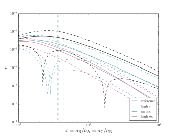
Figure 2: The ratio r𝑟r of the absolute value of the orbit-averaged octupole-order cross term in the Hamiltonian to the absolute value of all other orbit-averaged terms at octupole and hexadecupole order (cf. equation 2.4), plotted as a function of x=aB/aA=aC/aB𝑥subscript𝑎Bsubscript𝑎Asubscript𝑎Csubscript𝑎Bx=a_{\mathrm{B}}/a_{\mathrm{A}}=a_{\mathrm{C}}/a_{\mathrm{B}}. An averaging over the orientations of the three binaries has been carried out (assuming random orbital orientations), and four different combinations of masses and eccentricities are assumed, which are given in Table 1. Solid lines: mean values of r𝑟r for the different realizations of orbital orientations; (non-vertical) dashed lines: the same mean values, offset by the standard deviations (here, the absolute values are taken). Estimates for the minimum value of x𝑥x for dynamical stability (based on the Mardling & Aarseth 2001 criterion applied to the AB and BC binaries) for each combination of parameters are indicated with vertical dashed lines. Note that for some of the ‘high m4subscript𝑚4m_{4}’ and ‘high e𝑒e’ combinations, these values are >102absentsuperscript102>10^{2}, and are therefore beyond the range of the figure.
description m1subscript𝑚1m_{1} m2subscript𝑚2m_{2} m3subscript𝑚3m_{3} m4subscript𝑚4m_{4} eAsubscript𝑒Ae_{\mathrm{A}} eBsubscript𝑒Be_{\mathrm{B}} eCsubscript𝑒Ce_{\mathrm{C}}
reference 2 1 1 1 0.1 0.1 0.1
high e𝑒e 2 1 1 1 0.99 0.99 0.99
no oct 1 1 2 1 0.1 0.1 0.1
high m4subscript𝑚4m_{4} 2 1 1 106superscript10610^{6} 0.1 0.1 0.1
Table 1: Different combinations of the masses and eccentricities included in Fig. 2. Note that r𝑟r depends on the masses only through their ratios, hence the mass unit is arbitrary.

2.4 The importance of the octupole-order cross terms

In Section 2.1 we derived a cross term in the Hamiltonian at octupole order. Here, we investigate further the importance of this term with respect to other terms at the octupole and the next higher order, the hexacupole order. Long-term effects of the cross term can only be investigated by carrying out numerical integrations in time. However, a proxy for the short-term importance of the cross term is the ratio r𝑟r of the absolute value of the orbit-averaged cross term, to the absolute value of all other orbit-averaged terms at octupole and hexadecupole order, i.e.

rabs[H¯oct,cross(H¯oct,AB+H¯oct,BC+H¯oct,AC+H¯oct,cross\displaystyle r\equiv\mathrm{abs}\left[\,\overline{H}_{\mathrm{oct,\,cross}}\,\left(\overline{H}_{\mathrm{oct,AB}}+\overline{H}_{\mathrm{oct,BC}}+\overline{H}_{\mathrm{oct,AC}}+\overline{H}_{\mathrm{oct,\,cross}}\right.\right.
+H¯hd,AB+H¯hd,BC+H¯hd,AC+H¯hd,cross,1+H¯hd,cross,2)1].\displaystyle\left.\left.+\overline{H}_{\mathrm{hd,AB}}+\overline{H}_{\mathrm{hd,BC}}+\overline{H}_{\mathrm{hd,AC}}+\overline{H}_{\mathrm{hd,\,cross,1}}+\overline{H}_{\mathrm{hd,\,cross,2}}\right)^{-1}\right]. (10)

Here, H¯oct,klsubscript¯𝐻oct𝑘𝑙\overline{H}_{\mathrm{oct},kl} and H¯hd,klsubscript¯𝐻hd𝑘𝑙\overline{H}_{\mathrm{hd},kl} denote the orbit-averaged octupole-order and hexadecupole order terms corresponding to pair kl𝑘𝑙kl, respectively. They can be obtained directly from the general expressions equations (33c) and (33), and using the substitutions discussed above in Section 2.1.

In principle, r𝑟r can be maximized with respect to the parameters defining the properties and state of the quadruple system, i.e. with respect to the four misubscript𝑚𝑖m_{i} and the three aksubscript𝑎𝑘a_{k}, eksubscript𝑒𝑘e_{k}, 𝒆^ksubscript^𝒆𝑘\hat{\boldsymbol{e}}_{k} and 𝒋^ksubscript^𝒋𝑘\hat{\boldsymbol{j}}_{k} (with the orthogonality constraint 𝒆^k𝒋^k=0subscript^𝒆𝑘subscript^𝒋𝑘0\hat{\boldsymbol{e}}_{k}\cdot\hat{\boldsymbol{j}}_{k}=0). This would yield the largest possible contribution of the cross term. However, the dimensionality (25) of this problem is very large, and this makes it computationally very difficult to find the absolute maximum. Here, we simplify the problem by restricting the parameter space.

In particular, we set xaB/aA=aC/aB𝑥subscript𝑎Bsubscript𝑎Asubscript𝑎Csubscript𝑎Bx\equiv a_{\mathrm{B}}/a_{\mathrm{A}}=a_{\mathrm{C}}/a_{\mathrm{B}}, thereby reducing the dependence of the three semimajor axes to a single quantity. For given masses and eccentricities, we randomly sample the six unit vectors 𝒆^ksubscript^𝒆𝑘\hat{\boldsymbol{e}}_{k} and 𝒋^ksubscript^𝒋𝑘\hat{\boldsymbol{j}}_{k} with the orthogonality constraint 𝒆^k𝒋^k=0subscript^𝒆𝑘subscript^𝒋𝑘0\hat{\boldsymbol{e}}_{k}\cdot\hat{\boldsymbol{j}}_{k}=0. We compute r𝑟r for 20 of such realizations and each x𝑥x, and subsequently, we compute the mean and standard deviations.

In Fig. 2, we show the resulting mean values (solid lines) and mean values offset by the standard deviations (dashed lines) of r𝑟r as a function of x𝑥x. We include four different combinations of masses and eccentricities, which are enumerated in Table 1. The minimum value of x𝑥x for dynamical stability of the system is estimated by computing the critical semimajor axis ratio for stability of the AB and BC systems separately using the criterion of Mardling & Aarseth (2001). The latter two ratios are indicated for each combination of parameters in Fig. 2 with vertical dashed lines.

Regardless of our choice of parameters, r𝑟r is typically small, in the sense that for values of x𝑥x large enough for dynamical stability, r102less-than-or-similar-to𝑟superscript102r\lesssim 10^{-2}. For highly hierarchical systems, i.e. x100greater-than-or-equivalent-to𝑥100x\gtrsim 100, r104less-than-or-similar-to𝑟superscript104r\lesssim 10^{-4}. This indicates that typically the cross terms do not dominate the dynamics, at least for the short-term evolution. We note, however, that the octupole-order cross terms could give rise to important dynamical effects on long time-scales in less hierarchical systems.
Refer to caption
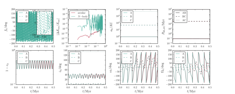
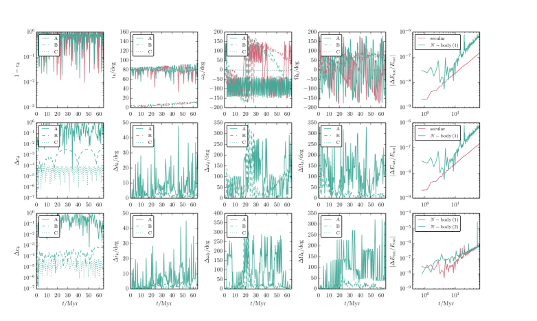
Figure 3: Comparison between the evolution of a quadruple system as computed with the orbit-averaged code SecularQuadruple developed in this work (red lines) and the direct N𝑁N-body code Mikkola (Mikkola & Merritt 2008; green lines). The assumed initial parameters were semimajor axes aA=1AUsubscript𝑎A1AUa_{\mathrm{A}}=1\,\mathrm{AU}, aB=5×10²AUsubscript𝑎B5superscript102AUa_{\mathrm{B}}=5\times 10^{2}\,\mathrm{AU} and aC=5×10³AUsubscript𝑎C5superscript103AUa_{\mathrm{C}}=5\times 10^{3}\,\mathrm{AU}, masses m1=m3=m4=1Msubscript𝑚1subscript𝑚3subscript𝑚41subscriptMdirect-productm_{1}=m_{3}=m_{4}=1\,\mathrm{M}_{\odot} and m2=0.5Msubscript𝑚20.5subscriptMdirect-productm_{2}=0.5\,\mathrm{M}_{\odot}, eccentricities eA=eB=eC=0.5subscript𝑒Asubscript𝑒Bsubscript𝑒C0.5e_{\mathrm{A}}=e_{\mathrm{B}}=e_{\mathrm{C}}=0.5, inclinations iA=45subscript𝑖Asuperscript45i_{\mathrm{A}}=45^{\circ}, iB=0subscript𝑖Bsuperscript0i_{\mathrm{B}}=0^{\circ}, iC=135subscript𝑖Csuperscript135i_{\mathrm{C}}=135^{\circ}, arguments of pericentre ωA=ωB=ωC=0subscript𝜔Asubscript𝜔Bsubscript𝜔Csuperscript0\omega_{\mathrm{A}}=\omega_{\mathrm{B}}=\omega_{\mathrm{C}}=0^{\circ} and longitudes of the ascending nodes ΩA=ΩB=ΩC=0subscriptΩAsubscriptΩBsubscriptΩCsuperscript0\Omega_{\mathrm{A}}=\Omega_{\mathrm{B}}=\Omega_{\mathrm{C}}=0^{\circ}. When applicable to a single binary, solid, dashed and dotted curves correspond binaries A, B and C, respectively. When applicable to a binary pair, solid, dashed and dotted curves correspond to the binary pairs AB, BC and AC, respectively. The quantity |ΔEtot/Etot|Δsubscript𝐸totsubscript𝐸tot|\Delta E_{\mathrm{tot}}/E_{\mathrm{tot}}| is the absolute value of relative error in the total energy (the orbit-averaged Hamiltonian in the case of SecularQuadruple), and fksubscript𝑓𝑘f_{k} is the true anomaly (applicable only to the N𝑁N-body simulations). The inset in the top-left panel shows a magnification between t=0𝑡0t=0 and 0.02 Myr. Note that the orbital period of binary A, PA0.8yrsubscript𝑃A0.8yrP_{\mathrm{A}}\approx 0.8\,\mathrm{yr}, is too short compared to the output resolution (500yrabsent500yr\approx 500\,\mathrm{yr}) for fAsubscript𝑓Af_{\mathrm{A}} to be resolved. Also note that in the orbit-averaged code, the semimajor axes are constant by assumption, whereas the KL time-scales PKL,klsubscript𝑃KL𝑘𝑙P_{\mathrm{KL},kl} in principle depend on time through the time-dependence of elsubscript𝑒𝑙e_{l} (cf. equation 11). However, in this case, the dependence is extremely weak and not visible in the top-right panel.
Refer to caption
Figure 4: Top row: comparison between the evolution as computed with the orbit-averaged code SecularQuadruple (red lines) and the direct N𝑁N-body code Mikkola (Mikkola & Merritt 2008; green lines). The system parameters are aA=1AUsubscript𝑎A1AUa_{\mathrm{A}}=1\mathrm{AU}, aB=102AUsubscript𝑎Bsuperscript102AUa_{\mathrm{B}}=10^{2}\,\mathrm{AU} and aC=5×10³AUsubscript𝑎C5superscript103AUa_{\mathrm{C}}=5\times 10^{3}\,\mathrm{AU}, m1=m3=m4=1Msubscript𝑚1subscript𝑚3subscript𝑚41subscriptMdirect-productm_{1}=m_{3}=m_{4}=1\,\mathrm{M}_{\odot} and m2=0.5Msubscript𝑚20.5subscriptMdirect-productm_{2}=0.5\,\mathrm{M}_{\odot}, eA=eB=eC=0.01subscript𝑒Asubscript𝑒Bsubscript𝑒C0.01e_{\mathrm{A}}=e_{\mathrm{B}}=e_{\mathrm{C}}=0.01, iA=iC=85subscript𝑖Asubscript𝑖Csuperscript85i_{\mathrm{A}}=i_{\mathrm{C}}=85^{\circ} and iB=0subscript𝑖Bsuperscript0i_{\mathrm{B}}=0^{\circ}, ωA=ωB=ωC=0subscript𝜔Asubscript𝜔Bsubscript𝜔Csuperscript0\omega_{\mathrm{A}}=\omega_{\mathrm{B}}=\omega_{\mathrm{C}}=0^{\circ} and ΩA=ΩB=ΩC=0subscriptΩAsubscriptΩBsubscriptΩCsuperscript0\Omega_{\mathrm{A}}=\Omega_{\mathrm{B}}=\Omega_{\mathrm{C}}=0^{\circ} (the same as in panels 1-6 of Fig. 6). Middle row: the differences in eksubscript𝑒𝑘e_{k}, iksubscript𝑖𝑘i_{k}, ωksubscript𝜔𝑘\omega_{k} and ΩksubscriptΩ𝑘\Omega_{k} between the secular code and one realization of the N𝑁N-body code, as a function of time. Bottom row: the differences in eksubscript𝑒𝑘e_{k}, iksubscript𝑖𝑘i_{k}, ωksubscript𝜔𝑘\omega_{k} and ΩksubscriptΩ𝑘\Omega_{k} between two realizations with the N𝑁N-body code with different initial orbital phases fksubscript𝑓𝑘f_{k}. Relative energy errors are shown in the last column.
eksubscript𝑒𝑘e_{k} ωksubscript𝜔𝑘\omega_{k} ΩksubscriptΩ𝑘\Omega_{k}
A B C A B C A B C
K-S pair D𝐷D p𝑝p D𝐷D p𝑝p D𝐷D p𝑝p D𝐷D p𝑝p D𝐷D p𝑝p D𝐷D p𝑝p D𝐷D p𝑝p D𝐷D p𝑝p D𝐷D p𝑝p
SN1 0.1 0.38 0.16 0.03 0.94 0.0 0.38 0.0 0.19 0.01 0.07 0.0 0.04 1.0 0.06 0.9 0.02 1.0
SNdelimited-⟨⟩SN\langle\mathrm{SN}\rangle 0.08 0.65 0.18 0.02 0.73 0.0 0.34 0.11 0.17 0.02 0.09 0.58 0.05 0.95 0.07 0.85 0.02 1.0
NN1 0.09 0.46 0.11 0.31 0.1 0.38 0.45 0.0 0.04 1.0 0.08 0.38 0.04 1.0 0.06 0.96 0.01 1.0
NNdelimited-⟨⟩NN\langle\mathrm{NN}\rangle 0.09 0.55 0.12 0.43 0.35 0.14 0.49 0.08 0.05 0.95 0.12 0.36 0.05 0.97 0.06 0.88 0.02 1.0
Table 2: Results of two-sided K-S tests (statistic D𝐷D and the p𝑝p-value) for time series in eksubscript𝑒𝑘e_{k}, ωksubscript𝜔𝑘\omega_{k} and ΩksubscriptΩ𝑘\Omega_{k} for the integrations shown in Fig. 4. In the first row, the secular code is compared to one realization of the N𝑁N-body code, Mikkola (Mikkola & Merritt, 2008). In the second row, the secular code is compared to five realizations of the N𝑁N-body code (i.e. with different initial mean anomalies), and given are the resulting values of D𝐷D and p𝑝p averaged over individual K-S tests. In the third row, two realizations of the N𝑁N-body code are compared, and in the fourth row, K-S tests are carried out for all combinations of the five realizations of the N𝑁N-body codes, and the quoted values of D𝐷D and p𝑝p are averaged over these combinations.

2.5 Comparisons to direct N𝑁N-body integrations

As a first demonstration of our algorithm, we show in Fig. 3 a comparison of a short-term integration with SecularQuadruple (red lines) and Mikkola (Mikkola & Merritt, 2008), a highly accurate direct N𝑁N-body code that uses chain regularization (green lines)222We remark that for this type of systems, it is essential to use a highly accurate N𝑁N-body code because a large number of orbits, in particular in binary A, needs to be integrated very accurately.. The assumed initial parameters were semimajor axes aA=1AUsubscript𝑎A1AUa_{\mathrm{A}}=1\,\mathrm{AU}, aB=5×10²AUsubscript𝑎B5superscript102AUa_{\mathrm{B}}=5\times 10^{2}\,\mathrm{AU}, aC=5×10³AUsubscript𝑎C5superscript103AUa_{\mathrm{C}}=5\times 10^{3}\,\mathrm{AU}, masses m1=m3=m4=1Msubscript𝑚1subscript𝑚3subscript𝑚41subscriptMdirect-productm_{1}=m_{3}=m_{4}=1\,\mathrm{M}_{\odot} and m2=0.5Msubscript𝑚20.5subscriptMdirect-productm_{2}=0.5\,\mathrm{M}_{\odot}, eccentricities eA=eB=eC=0.5subscript𝑒Asubscript𝑒Bsubscript𝑒C0.5e_{\mathrm{A}}=e_{\mathrm{B}}=e_{\mathrm{C}}=0.5, inclinations iA=45subscript𝑖Asuperscript45i_{\mathrm{A}}=45^{\circ}, iB=0subscript𝑖Bsuperscript0i_{\mathrm{B}}=0^{\circ} and iC=135subscript𝑖Csuperscript135i_{\mathrm{C}}=135^{\circ}, arguments of pericentre ωA=ωB=ωC=0subscript𝜔Asubscript𝜔Bsubscript𝜔Csuperscript0\omega_{\mathrm{A}}=\omega_{\mathrm{B}}=\omega_{\mathrm{C}}=0^{\circ} and longitudes of the ascending nodes ΩA=ΩB=ΩC=0subscriptΩAsubscriptΩBsubscriptΩCsuperscript0\Omega_{\mathrm{A}}=\Omega_{\mathrm{B}}=\Omega_{\mathrm{C}}=0^{\circ}. Initially, i.e. during the first few KL oscillations in the AB pair, the two methods show very good agreement. However, as time progresses, noticeable deviations develop.

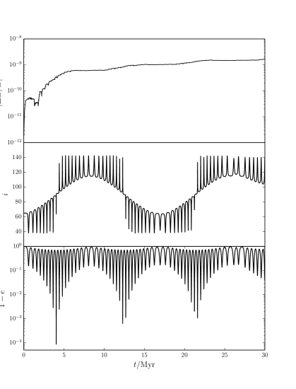
This poses a problem when comparing the two methods in longer integrations, i.e. for time-scales PKL,ABmuch-greater-thanabsentsubscript𝑃KLAB\gg P_{\mathrm{KL,AB}}, where PKL,ABsubscript𝑃KLABP_{\mathrm{KL,AB}} is the KL time-scale for the AB binary pair (cf. equation 11 below). To illustrate this, we show in the top row in Fig. 4 another example, where the integration time is 60PKL,ABsimilar-toabsent60subscript𝑃KLAB\sim 60\,P_{\mathrm{KL,AB}}. In this case, we set aA=1AUsubscript𝑎A1AUa_{\mathrm{A}}=1\mathrm{AU}, aB=102AUsubscript𝑎Bsuperscript102AUa_{\mathrm{B}}=10^{2}\,\mathrm{AU} and aC=5×10³AUsubscript𝑎C5superscript103AUa_{\mathrm{C}}=5\times 10^{3}\,\mathrm{AU}, m1=m3=m4=1Msubscript𝑚1subscript𝑚3subscript𝑚41subscriptMdirect-productm_{1}=m_{3}=m_{4}=1\,\mathrm{M}_{\odot} and m2=0.5Msubscript𝑚20.5subscriptMdirect-productm_{2}=0.5\,\mathrm{M}_{\odot}, eA=eB=eC=0.01subscript𝑒Asubscript𝑒Bsubscript𝑒C0.01e_{\mathrm{A}}=e_{\mathrm{B}}=e_{\mathrm{C}}=0.01, iA=iC=85subscript𝑖Asubscript𝑖Csuperscript85i_{\mathrm{A}}=i_{\mathrm{C}}=85^{\circ} and iB=0subscript𝑖Bsuperscript0i_{\mathrm{B}}=0^{\circ}, ωA=ωB=ωC=0subscript𝜔Asubscript𝜔Bsubscript𝜔Csuperscript0\omega_{\mathrm{A}}=\omega_{\mathrm{B}}=\omega_{\mathrm{C}}=0^{\circ} and ΩA=ΩB=ΩC=0subscriptΩAsubscriptΩBsubscriptΩCsuperscript0\Omega_{\mathrm{A}}=\Omega_{\mathrm{B}}=\Omega_{\mathrm{C}}=0^{\circ} (note that this system is the same as in panels 1-6 of Fig. 6). In the top row of Fig. 4, the quantities eksubscript𝑒𝑘e_{k}, iksubscript𝑖𝑘i_{k}, ωksubscript𝜔𝑘\omega_{k}, ΩksubscriptΩ𝑘\Omega_{k} and the relative energy errors, pertaining to integrations with SecularQuadruple (Mikkola), are shown with red (green) lines. The differences in eksubscript𝑒𝑘e_{k}, iksubscript𝑖𝑘i_{k}, ωksubscript𝜔𝑘\omega_{k} and ΩksubscriptΩ𝑘\Omega_{k} between the integrations with these codes are shown as a function of time in the middle row in Fig. 4. In this case, there is clearly no longer a one-to-one agreement between the two methods.

When comparing these results on long time-scales (i.e. long compared to PKL,ABsubscript𝑃KLABP_{\mathrm{KL,AB}}), it is important to take into account that for this system, the phase of the KL cycle in binary A becomes inherently chaotic on a time-scale that is shorter than PKL,ABsubscript𝑃KLABP_{\mathrm{KL,AB}}. To establish this, we determined the Lyapunov time-scale by carrying out pairs of integrations where in one realization, the initial value of eA=0.01subscript𝑒A0.01e_{\mathrm{A}}=0.01, was increased by ΔeA(0)=104Δsubscript𝑒A0superscript104\Delta e_{\mathrm{A}}(0)=10^{-4}. We found that the difference ΔeA(t)Δsubscript𝑒A𝑡\Delta e_{\mathrm{A}}(t) between the two integrations initially shows an exponential behaviour as a function of time. Subsequently, we fitted log[ΔeA(t)/ΔeA(0)]Δsubscript𝑒A𝑡Δsubscript𝑒A0\log[\Delta e_{\mathrm{A}}(t)/\Delta e_{\mathrm{A}}(0)] with time assuming a linear relation, i.e. log[ΔeA(t)/ΔeA(0)]=C+λtΔsubscript𝑒A𝑡Δsubscript𝑒A0𝐶𝜆𝑡\log[\Delta e_{\mathrm{A}}(t)/\Delta e_{\mathrm{A}}(0)]=C+\lambda t where C𝐶C is a constant, and we determined the Lyapunov time-scale tLysubscript𝑡Lyt_{\mathrm{Ly}} from the inverse of the resulting slope, i.e. tLy=λ1subscript𝑡Lysuperscript𝜆1t_{\mathrm{Ly}}=\lambda^{-1}.

We find a Lyapunov time-scale of tLy0.11Myrsubscript𝑡Ly0.11Myrt_{\mathrm{Ly}}\approx 0.11\,\mathrm{Myr} for this system, and this value is the same for either the secular and direct codes. Reducing the accuracy in the secular integrations does not affect the result, unless the accuracy is reduced such that the relative energy errors increase to >0.1absent0.1>0.1. We also verified that tL0.11Myrsubscript𝑡L0.11Myrt_{\mathrm{L}}\approx 0.11\,\mathrm{Myr} for integrations with another N𝑁N-body code, Sakura (Gonçalves Ferrari et al., 2014).

This value of 0.11Myr0.11Myr0.11\,\mathrm{Myr} is shorter than PKL,AB1Myrsubscript𝑃KLAB1MyrP_{\mathrm{KL,AB}}\approx 1\,\mathrm{Myr}, which suggests that the system is chaotic on a short time-scale. However, we find that this chaoticity arises from a slightly different phase of the KL cycle between the integrations with ΔeA(0)=104Δsubscript𝑒A0superscript104\Delta e_{\mathrm{A}}(0)=10^{-4}, whereas the shape of the eA(t)subscript𝑒A𝑡e_{\mathrm{A}}(t) remains essentially the same. This result suggests that for long time-scales, it is not meaningful to compare the secular and N𝑁N-body integrations on a one-to-one basis. However, given that the chaotic behaviour discussed above is associated with the phase of the KL cycle, it should still be appropriate to compare the two methods statistically.

We also note that when comparing the two methods, it is important to take into account that in the N𝑁N-body integrations, there is an additional dependence on the three initial orbital phases. We have also carried out N𝑁N-body integrations with different initial orbital phases, where the initial mean anomaly was sampled randomly. We show the differences between two different N𝑁N-body realizations as a function of time in the bottom row in Fig. 4. These differences are typically at least as large as the differences between the secular code, and a single realization with the N𝑁N-body code. Furthermore, we have determined the Lyapunov time-scale as described above, where now ΔeA(t)Δsubscript𝑒A𝑡\Delta e_{\mathrm{A}}(t) was determined from two short-term N𝑁N-body integrations with different random mean anomalies. Again, we find that ΔeAΔsubscript𝑒A\Delta e_{\mathrm{A}} increases exponentially with time, with a Lyapunov time-scale of tLy0.1Myrsubscript𝑡Ly0.1Myrt_{\mathrm{Ly}}\approx 0.1\,\mathrm{Myr}. Therefore, the differences between the direct N𝑁N-body integrations with different initial orbital phases can be ascribed to the chaotic nature of the phase of the KL cycles.

In Table 2, we show results of two-sided Kolmogorov-Smirnov (K-S) tests (Kolmogorov, 1933; Smirnov, 1948) between time series in eksubscript𝑒𝑘e_{k}, ωksubscript𝜔𝑘\omega_{k} and ΩksubscriptΩ𝑘\Omega_{k} obtained from the integration carried out with the secular code, and the integration of five different realizations with the N𝑁N-body code (i.e. with different initial mean anomalies). For K-S tests between the secular and N𝑁N-body integrations, and K-S tests between N𝑁N-body integrations with different realizations, the D𝐷D-values are generally low and the p𝑝p-values are typically high. This shows that the integrations between the secular and N𝑁N-body integrations are statistically consistent, and that the same applies to the N𝑁N-body integrations with different realizations.

We conclude that, for the highly hierarchical systems considered here, the secular code gives results that are statistically consistent with the direct N𝑁N-body code. The much greater speed makes the former highly suited for the long-term study of a large number of systems. For example, the integration with SecularQuadruple for one of the systems in Fig. 4 is 104similar-toabsentsuperscript104\sim 10^{4} times faster compared to Mikkola.

3 Global evolution of highly hierarchical systems

In principle, the SecularQuadruple algorithm can be used to perform a systematic parameter space study. Instead, here we choose to focus in detail on particular configurations to get insight into the typically complex dynamics that can arise. We consider the following two cases: (1) binaries A and B are initially coplanar (iAB,0=0subscript𝑖AB0superscript0i_{\mathrm{AB,0}}=0^{\circ}) and highly inclined with respect to binary C (iBC,0=85subscript𝑖BC0superscript85i_{\mathrm{BC,0}}=85^{\circ}), and (2) binaries A and B are initially highly inclined (iAB,0=85subscript𝑖AB0superscript85i_{\mathrm{AB,0}}=85^{\circ}) while binary B is also highly inclined with respect to binary C (iBC,0=85subscript𝑖BC0superscript85i_{\mathrm{BC,0}}=85^{\circ}). In both cases, we assume that the quadruple system is highly hierarchical at all times, i.e. rp,Arp,Brp,Cmuch-less-thansubscript𝑟pAsubscript𝑟pBmuch-less-thansubscript𝑟pCr_{\mathrm{p,A}}\ll r_{\mathrm{p,B}}\ll r_{\mathrm{p,C}}, where rp,ksubscript𝑟p𝑘r_{\mathrm{p},k} is the pericentre distance in binary k𝑘k.

For both cases (1) and (2), we performed a sequence of integrations in which aAsubscript𝑎Aa_{\mathrm{A}} was varied between 103superscript10310^{-3} and 1 AU, and all other initial parameters were kept fixed. The latter were assumed to be semimajor axes aB=102AUsubscript𝑎Bsuperscript102AUa_{\mathrm{B}}=10^{2}\,\mathrm{AU} and aC=5×10³AUsubscript𝑎C5superscript103AUa_{\mathrm{C}}=5\times 10^{3}\,\mathrm{AU}, masses m1=m3=m4=1Msubscript𝑚1subscript𝑚3subscript𝑚41subscriptMdirect-productm_{1}=m_{3}=m_{4}=1\,\mathrm{M}_{\odot} and m2=0.5Msubscript𝑚20.5subscriptMdirect-productm_{2}=0.5\,\mathrm{M}_{\odot}, eccentricities eA=eB=eC=0.01subscript𝑒Asubscript𝑒Bsubscript𝑒C0.01e_{\mathrm{A}}=e_{\mathrm{B}}=e_{\mathrm{C}}=0.01, arguments of pericentre ωA=ωB=ωC=0subscript𝜔Asubscript𝜔Bsubscript𝜔Csuperscript0\omega_{\mathrm{A}}=\omega_{\mathrm{B}}=\omega_{\mathrm{C}}=0^{\circ} and longitudes of the ascending nodes ΩA=ΩB=ΩC=0subscriptΩAsubscriptΩBsubscriptΩCsuperscript0\Omega_{\mathrm{A}}=\Omega_{\mathrm{B}}=\Omega_{\mathrm{C}}=0^{\circ}. The integration time for each system was set to 20PKL,BC,020subscript𝑃KLBC020\,P_{\mathrm{KL,BC,0}}, where PKL,BC,0subscript𝑃KLBC0P_{\mathrm{KL,BC,0}} is the initial KL time-scale applied to binaries B and C, which we approximate by (Innanen et al., 1997)

PKL,kl=Pl2Pkmk,p+mk,s+ml,sml,s(1el2)3/2,subscript𝑃KL𝑘𝑙superscriptsubscript𝑃𝑙2subscript𝑃𝑘subscript𝑚𝑘psubscript𝑚𝑘ssubscript𝑚𝑙ssubscript𝑚𝑙ssuperscript1superscriptsubscript𝑒𝑙232\displaystyle P_{\mathrm{KL},kl}=\frac{P_{l}^{2}}{P_{k}}\frac{m_{k,\mathrm{p}}+m_{k,\mathrm{s}}+m_{l,\mathrm{s}}}{m_{l,\mathrm{s}}}\left(1-e_{l}^{2}\right)^{3/2}, (11)

where mk,p=m1subscript𝑚𝑘psubscript𝑚1m_{k,\mathrm{p}}=m_{1}, mk,s=m2subscript𝑚𝑘ssubscript𝑚2m_{k,\mathrm{s}}=m_{2} and ml,s=m3subscript𝑚𝑙ssubscript𝑚3m_{l,\mathrm{s}}=m_{3} in the case of PKL,ABsubscript𝑃KLABP_{\mathrm{KL,AB}}, and mk,p=m1+m2subscript𝑚𝑘psubscript𝑚1subscript𝑚2m_{k,\mathrm{p}}=m_{1}+m_{2}, mk,s=m3subscript𝑚𝑘ssubscript𝑚3m_{k,\mathrm{s}}=m_{3} and ml,s=m4subscript𝑚𝑙ssubscript𝑚4m_{l,\mathrm{s}}=m_{4} in the case of PKL,BCsubscript𝑃KLBCP_{\mathrm{KL,BC}} (cf. Section 2.1). Note that, contrary to triple systems and at the quadrupole-order approximation, the ‘outer’ orbit eccentricity elsubscript𝑒𝑙e_{l} in equation (11) can change in time if this equation is applied to binaries A and B. This is addressed in more detail below.

For hierarchical triple systems, the octupole parameter

ϵoctm1m2m1+m2ainaouteout1eout2subscriptitalic-ϵoctsubscript𝑚1subscript𝑚2subscript𝑚1subscript𝑚2subscript𝑎insubscript𝑎outsubscript𝑒out1superscriptsubscript𝑒out2\displaystyle\epsilon_{\mathrm{oct}}\equiv\frac{m_{1}-m_{2}}{m_{1}+m_{2}}\frac{a_{\mathrm{in}}}{a_{\mathrm{out}}}\frac{e_{\mathrm{out}}}{1-e_{\mathrm{out}}^{2}} (12)

is a useful proxy for the importance of octupole-order effects, in particular, orbital flips. The latter can occur if ϵoct103greater-than-or-equivalent-tosubscriptitalic-ϵoctsuperscript103\epsilon_{\mathrm{oct}}\gtrsim 10^{-3}, and are typically associated with very high eccentricities (Lithwick & Naoz, 2011; Katz et al., 2011; Teyssandier et al., 2013; Li et al., 2014b). In the systems considered here, the initial octupole parameters ϵoctsubscriptitalic-ϵoct\epsilon_{\mathrm{oct}} range between 3.3×10⁸absent3.3superscript108\approx 3.3\times 10^{-8} and 3.3×10⁵absent3.3superscript105\approx 3.3\times 10^{-5} for binary pair AB; for binary pair BC, ϵoct4.0×105subscriptitalic-ϵoct4.0superscript105\epsilon_{\mathrm{oct}}\approx 4.0\times 10^{-5}. This indicates that octupole-order terms are not important. Furthermore, the initial ratio r0subscript𝑟0r_{0} of the orbit-averaged octupole-order cross term to all other orbit-averaged terms at octupole and hexadecupole order (cf. Section 2.4) ranges between 2×10¹²absent2superscript1012\approx 2\times 10^{-12} and 3×10⁷absent3superscript107\approx 3\times 10^{-7}, indicating that the orbit-averaged octupole-order cross term can similarly be neglected. The results presented below therefore demonstrate the dynamics that are manifested at the lowest possible, i.e. quadrupole, order.

3.1 Examples: A and B initially coplanar
Refer to caption
Refer to caption
Refer to caption
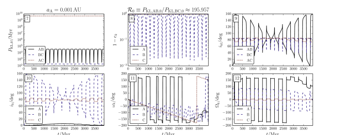
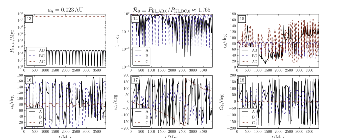
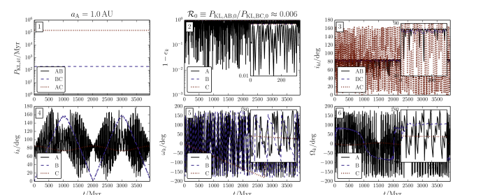
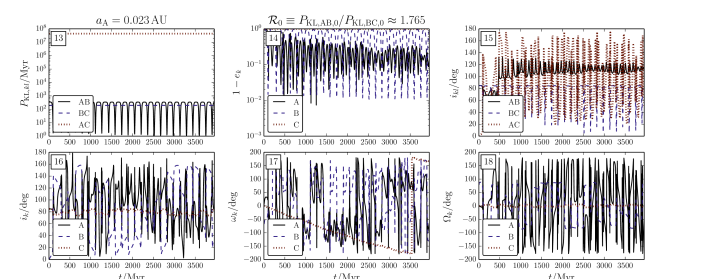
Figure 5: Evolution of three quadruple systems as discussed in Section 3.1, computed with SecularQuadruple. Binaries A and B are initially coplanar (as opposed to highly inclined in Fig. 6). Reference numbers are shown in the top left of each panel. Panels 1-6, 7-12 and 13-18 correspond to semimajor axes of binary A of 1, 0.001 and 0.023 AU, respectively. The other initial parameters are the same for these groups of panels, and are given by semimajor axes aB=102AUsubscript𝑎Bsuperscript102AUa_{\mathrm{B}}=10^{2}\,\mathrm{AU} and aC=5×10³AUsubscript𝑎C5superscript103AUa_{\mathrm{C}}=5\times 10^{3}\,\mathrm{AU}, masses m1=m3=m4=1Msubscript𝑚1subscript𝑚3subscript𝑚41subscriptMdirect-productm_{1}=m_{3}=m_{4}=1\,\mathrm{M}_{\odot} and m2=0.5Msubscript𝑚20.5subscriptMdirect-productm_{2}=0.5\,\mathrm{M}_{\odot}, eccentricities eA=eB=eC=0.01subscript𝑒Asubscript𝑒Bsubscript𝑒C0.01e_{\mathrm{A}}=e_{\mathrm{B}}=e_{\mathrm{C}}=0.01, inclinations iA=iB=0subscript𝑖Asubscript𝑖Bsuperscript0i_{\mathrm{A}}=i_{\mathrm{B}}=0^{\circ}, iC=85subscript𝑖Csuperscript85i_{\mathrm{C}}=85^{\circ}, arguments of pericentre ωA=ωB=ωC=0subscript𝜔Asubscript𝜔Bsubscript𝜔Csuperscript0\omega_{\mathrm{A}}=\omega_{\mathrm{B}}=\omega_{\mathrm{C}}=0^{\circ} and longitudes of the ascending nodes ΩA=ΩB=ΩC=0subscriptΩAsubscriptΩBsubscriptΩCsuperscript0\Omega_{\mathrm{A}}=\Omega_{\mathrm{B}}=\Omega_{\mathrm{C}}=0^{\circ}. In panels 2 and 5, the abscissae in the inset range between t=0𝑡0t=0 and 200 Myr.
Refer to caption
Refer to caption
Refer to caption
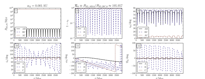
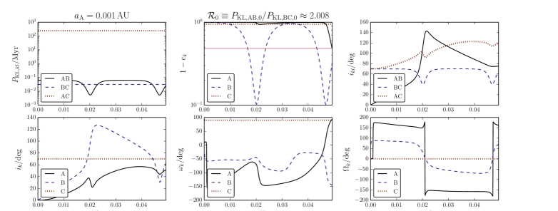
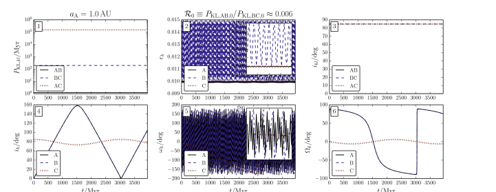
Figure 6: Evolution of three quadruple systems as discussed in Section 3.2, computed with SecularQuadruple. Binaries A and B are initially inclined by 85superscript8585^{\circ} (as opposed to 0superscript00^{\circ} in Fig. 5). Panels 1-6, 7-12 and 13-18 correspond to semimajor axes of binary A of 1, 0.001 and 0.023 AU, respectively. The other parameters are the same for these groups of panels, and are given by semimajor axes aB=102AUsubscript𝑎Bsuperscript102AUa_{\mathrm{B}}=10^{2}\,\mathrm{AU} and aC=5×10³AUsubscript𝑎C5superscript103AUa_{\mathrm{C}}=5\times 10^{3}\,\mathrm{AU}, masses m1=m3=m4=1Msubscript𝑚1subscript𝑚3subscript𝑚41subscriptMdirect-productm_{1}=m_{3}=m_{4}=1\,\mathrm{M}_{\odot} and m2=0.5Msubscript𝑚20.5subscriptMdirect-productm_{2}=0.5\,\mathrm{M}_{\odot}, eccentricities eA=eB=eC=0.01subscript𝑒Asubscript𝑒Bsubscript𝑒C0.01e_{\mathrm{A}}=e_{\mathrm{B}}=e_{\mathrm{C}}=0.01, inclinations iA=iC=85subscript𝑖Asubscript𝑖Csuperscript85i_{\mathrm{A}}=i_{\mathrm{C}}=85^{\circ}, iB=0subscript𝑖Bsuperscript0i_{\mathrm{B}}=0^{\circ}, arguments of pericentre ωA=ωB=ωC=0subscript𝜔Asubscript𝜔Bsubscript𝜔Csuperscript0\omega_{\mathrm{A}}=\omega_{\mathrm{B}}=\omega_{\mathrm{C}}=0^{\circ} and longitudes of the ascending nodes ΩA=ΩB=ΩC=0subscriptΩAsubscriptΩBsubscriptΩCsuperscript0\Omega_{\mathrm{A}}=\Omega_{\mathrm{B}}=\Omega_{\mathrm{C}}=0^{\circ}. In panels 2, 3, 5 and 6, the abscissae in the insets range between t=0𝑡0t=0 and 300 Myr.

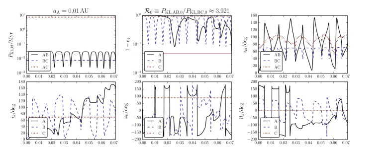
In our first case, iAB,0=0subscript𝑖AB0superscript0i_{\mathrm{AB,0}}=0^{\circ} and iBC,0=85subscript𝑖BC0superscript85i_{\mathrm{BC,0}}=85^{\circ}, which is achieved by setting the initial iA=iB=0subscript𝑖Asubscript𝑖Bsuperscript0i_{\mathrm{A}}=i_{\mathrm{B}}=0^{\circ} and iC=85subscript𝑖Csuperscript85i_{\mathrm{C}}=85^{\circ} (note that, initially, ΩA=ΩB=ΩCsubscriptΩAsubscriptΩBsubscriptΩC\Omega_{\mathrm{A}}=\Omega_{\mathrm{B}}=\Omega_{\mathrm{C}}). In the absence of the fourth body, there would not be any excitation of the eccentricity in binaries A and B because they are not mutually inclined and only the quadrupole-order terms are important. We note that if the initial eB=0.01subscript𝑒B0.01e_{\mathrm{B}}=0.01 were much larger (and therefore ϵoctsubscriptitalic-ϵoct\epsilon_{\mathrm{oct}} would be much higher, cf. equation 12), owing to the greater importance of the octupole-order terms, orbital flips and very high eccentricity oscillations in binary A would be possible in certain conditions, even if iAB,0subscript𝑖AB0i_{\mathrm{AB,0}} is close to zero (Li et al., 2014a). We show in Fig. 5 three examples of numerically integrated systems, in which aAsubscript𝑎Aa_{\mathrm{A}} is either 1 (panels 1-6), 0.001 (panels 7-12) or 0.023 AU (panels 13-18).

For aA=1AUsubscript𝑎A1AUa_{\mathrm{A}}=1\,\mathrm{AU}, the mutual inclination between binaries A and B, iABsubscript𝑖ABi_{\mathrm{AB}}, remains zero (cf. the solid line in panel 3 of Fig. 5). However, the individual inclinations of binaries A and B, iAsubscript𝑖Ai_{\mathrm{A}} and iBsubscript𝑖Bi_{\mathrm{B}}, which are initially zero, do change (cf. the solid and dashed lines in panel 4 of Fig. 5; note that these curves overlap). This can be understood from the large torque of binary B on binary A, compared to the torque of binary C on binary B. More quantitatively, the KL time-scales can be interpreted as proxies for the importance of these torques, and the initial KL time-scale for binaries A and B, PKL,AB,01.2Myrsubscript𝑃KLAB01.2MyrP_{\mathrm{KL,AB,0}}\approx 1.2\,\mathrm{Myr}, is much shorter (i.e. corresponding to a larger torque) than the initial KL time-scale for binaries B and C, PKL,BC,02×102Myrsubscript𝑃KLBC02superscript102MyrP_{\mathrm{KL,BC,0}}\approx 2\times 10^{2}\,\mathrm{Myr}. The large torque of binary B on binary A enforces that zero mutual inclination between these binaries is maintained, despite the torque from binary C on binary B. The latter torque changes the individual inclination of binary B on the time-scale of PKL,BCPKL,ABmuch-greater-thansubscript𝑃KLBCsubscript𝑃KLABP_{\mathrm{KL,BC}}\gg P_{\mathrm{KL,AB}}. Note that the mutual inclination is determined by the individual inclinations iksubscript𝑖𝑘i_{k} and longitudes of the ascending nodes ΩksubscriptΩ𝑘\Omega_{k} (cf. equation 7). Therefore, both these angles for binaries A and B follow each other very closely (cf. panels 4 and 6 of Fig. 5).

If binary A were replaced by a point mass, the eccentricity in binary B would oscillate as a result of the torque from binary C, with maxima of 1eB,max1021subscript𝑒Bsuperscript1021-e_{\mathrm{B,\max}}\approx 10^{-2}. However, in the case of a quadruple system, the short KL time-scale in binary A with binary B causes rapid precession in both binaries A and B, on roughly the same time-scale (cf. the black solid and blue dashed lines in panel 5 of Fig. 5). Consequently, the rapid precession in binary B quenches any KL oscillations induced by the torque of binary C. This effect is analogous to the quenching of KL oscillations in triple systems due to additional sources of periapse precession. Here, the additional precession is due to the extended nature of one of the components in the inner binary, rather than due to e.g. relativistic precession or tidal bulges. This quenching effect is discussed more quantitatively below, in Section 3.4.

In panels 7-12 of Fig. 5, we show the evolution of an example system with aA=103AUsubscript𝑎Asuperscript103AUa_{\mathrm{A}}=10^{-3}\,\mathrm{AU}. The initial KL time-scale for binaries A and B is PKL,AB,039GyrPKL,BC,02×102Myrsubscript𝑃KLAB039Gyrmuch-greater-thansubscript𝑃KLBC02superscript102MyrP_{\mathrm{KL,AB,0}}\approx 39\,\mathrm{Gyr}\gg P_{\mathrm{KL,BC,0}}\approx 2\times 10^{2}\,\mathrm{Myr}. Therefore, there is no induced precession of binary A on binary B, and KL eccentricity oscillations occur in binary B with maxima of 1eB,max1021subscript𝑒Bsuperscript1021-e_{\mathrm{B,\max}}\approx 10^{-2} (cf. the dashed lines in panel 8 of Fig. 5). Furthermore, the torque of binary C on binary B dominates compared to the torque of binary B on binary A. Consequently, the inclination of binary B changes rapidly, whereas the inclination of binary A hardly changes (cf. the solid and dashed lines in panel 10 of Fig. 5). However, this also changes the mutual inclination iABsubscript𝑖ABi_{\mathrm{AB}} between binaries A and B. The latter increases very rapidly (cf. the solid line in panel 9 of Fig. 5). Nevertheless, binaries A and B are only highly mutually inclined (iABsubscript𝑖ABi_{\mathrm{AB}} close to 90superscript9090^{\circ}) for short periods of time, and therefore, no significant eccentricity oscillations occur in binary A. In other words, the latter oscillations are impeded by rapid changes of the mutual inclination between binaries A and B, because of KL oscillations induced by binary C.

Finally, in panels 13-18 of Fig. 5, aA0.023AUsubscript𝑎A0.023AUa_{\mathrm{A}}\approx 0.023\,\mathrm{AU}. The initial KL time-scales for the binary pairs AB and BC are comparable, i.e. PKL,AB,03×102MyrPKL,BC,02×102Myrsubscript𝑃KLAB03superscript102Myrsimilar-tosubscript𝑃KLBC02superscript102MyrP_{\mathrm{KL,AB,0}}\approx 3\times 10^{2}\,\mathrm{Myr}\sim P_{\mathrm{KL,BC,0}}\approx 2\times 10^{2}\,\mathrm{Myr}, and therefore the torques of binary B on binary A and of binary C on binary B are also comparable. Binaries A and B become mutually inclined, and the KL time-scale for the AB pair is short enough for large excitation of the eccentricity of binary A. The result is a complex evolution in which the oscillations in eAsubscript𝑒Ae_{\mathrm{A}} are highly non-regular and strongly coupled with the oscillations of eBsubscript𝑒Be_{\mathrm{B}}. Interestingly, although binaries A and B started out with a mutual inclination of iAB,0=85<90subscript𝑖AB0superscript85superscript90i_{\mathrm{AB,0}}=85^{\circ}<90^{\circ}, the orientation between binaries A and B at t400Myrsimilar-to𝑡400Myrt\sim 400\,\mathrm{Myr} changes from prograde to retrograde. Such orbital flips also occur at later times, and are associated with high eccentricities in binary A. The evolution of the eccentricity of binary B is also affected, although the effect is much smaller and the oscillations can still be considered as regular. In Section 3.4, we study the effect of the eccentricity of binary B in more detail.

3.2 Examples: A and B initially highly inclined

In our second case, we assume that both binaries A and B and binaries B and C are initially highly inclined, i.e. iAB,0=85subscript𝑖AB0superscript85i_{\mathrm{AB,0}}=85^{\circ} and iBC,0=85subscript𝑖BC0superscript85i_{\mathrm{BC,0}}=85^{\circ}, which is achieved by setting iA=iC=85subscript𝑖Asubscript𝑖Csuperscript85i_{\mathrm{A}}=i_{\mathrm{C}}=85^{\circ} and iB=0subscript𝑖Bsuperscript0i_{\mathrm{B}}=0^{\circ}. The evolution of three example systems, with other parameters identical to those in Section 3.1, is shown in Fig. 6. In the absence of the fourth body, high-eccentricity KL oscillations would be induced in binary A.

For aA=1AUsubscript𝑎A1AUa_{\mathrm{A}}=1\,\mathrm{AU} (panels 1-6 of Fig. 6), PKL,ABPKL,BCmuch-less-thansubscript𝑃KLABsubscript𝑃KLBCP_{\mathrm{KL,AB}}\ll P_{\mathrm{KL,BC}}, and for time-scales comparable to PKL,ABsubscript𝑃KLABP_{\mathrm{KL,AB}}, KL eccentricity oscillations in binaries A and B are hardly affected by the torque of binary C. On much longer time-scales comparable to PKL,BCsubscript𝑃KLBCP_{\mathrm{KL,BC}}, iBsubscript𝑖Bi_{\mathrm{B}} changes because of the torque of binary C (cf. the blue dashed line in panel 4 of Fig. 6). However, the KL eccentricity oscillations between binaries A and B are not noticeably affected (note that in panels 2-6 of Fig. 6, the KL oscillations associated with binaries A and B are undersampled). Consequently, iAsubscript𝑖Ai_{\mathrm{A}}, iBsubscript𝑖Bi_{\mathrm{B}}, ΩAsubscriptΩA\Omega_{\mathrm{A}} and ΩBsubscriptΩB\Omega_{\mathrm{B}} are modulated on the PKL,BCsubscript𝑃KLBCP_{\mathrm{KL,BC}} time-scale. We note that, as a consequence of KL oscillations in the AB pair, there is still short-time-scale precession induced on binary B, preventing any eccentricity excitation in binary B. This is similar to the previous case when binaries A and B are initially coplanar.

For aA=0.001AUsubscript𝑎A0.001AUa_{\mathrm{A}}=0.001\,\mathrm{AU} (panels 7-12 of Fig. 6), the evolution is qualitatively very similar to the case when iAB,0=0subscript𝑖AB0superscript0i_{\mathrm{AB,0}}=0^{\circ}. This may be surprising, given the high initial mutual inclination between binaries A and B. However, the latter changes strongly on the much shorter time-scale of PKL,BCsubscript𝑃KLBCP_{\mathrm{KL,BC}}, and this prevents any eccentricity excitation in binary A. Note that in this case, the quenching of KL eccentricity oscillations in binary A is not due to induced precession. As can be seen in panel 11 of Fig. 6, ωAsubscript𝜔A\omega_{\mathrm{A}} is not much affected on the PKL,BCsubscript𝑃KLBCP_{\mathrm{KL,BC}} time-scale, although there is also a trend on a much longer time-scale of 4×10³similar-toabsent4superscript103\sim 4\times 10^{3} Myr. The KL time-scale for the AB pair changes periodically as eBsubscript𝑒Be_{\mathrm{B}} oscillates (cf. panel 7 of Fig. 6). Therefore the time-scale of 4×10³similar-toabsent4superscript103\sim 4\times 10^{3} Myr can, in this case, be interpreted as an effective KL time-scale for the AB pair.

When the KL time-scales for the AB and BC pairs are similar (cf. panels 13-18 of Fig. 6), the evolution of eAsubscript𝑒Ae_{\mathrm{A}} is complex and high eccentricities are attained, similarly to the case when iAB,0=0subscript𝑖AB0superscript0i_{\mathrm{AB,0}}=0^{\circ}. Again, an orbital flip occurs around t400similar-to𝑡400t\sim 400 Myr. Interestingly, subsequently there are no orbital flips, and the amplitude of the oscillations in eAsubscript𝑒Ae_{\mathrm{A}} and iABsubscript𝑖ABi_{\mathrm{AB}} gradually decreases.

3.3 Qualitative trends

The above examples suggest that the ratio of the (initial) KL time-scales for the AB and BC pairs,

0subscript0\displaystyle\mathcal{R}_{0} PKL,AB,0PKL,BC,0absentsubscript𝑃KLAB0subscript𝑃KLBC0\displaystyle\equiv\frac{P_{\mathrm{KL,AB,0}}}{P_{\mathrm{KL,BC,0}}}
=(aB3aAaC2)3/2(m1+m2m1+m2+m3)1/2m4m3(1eB,021eC,02)3/2,absentsuperscriptsuperscriptsubscript𝑎B3subscript𝑎Asuperscriptsubscript𝑎C232superscriptsubscript𝑚1subscript𝑚2subscript𝑚1subscript𝑚2subscript𝑚312subscript𝑚4subscript𝑚3superscript1superscriptsubscript𝑒B021superscriptsubscript𝑒C0232\displaystyle=\left(\frac{a_{\mathrm{B}}^{3}}{a_{\mathrm{A}}a_{\mathrm{C}}^{2}}\right)^{3/2}\left(\frac{m_{1}+m_{2}}{m_{1}+m_{2}+m_{3}}\right)^{1/2}\frac{m_{4}}{m_{3}}\left(\frac{1-e_{\mathrm{B,0}}^{2}}{1-e_{\mathrm{C,0}}^{2}}\right)^{3/2}, (13)

is an indication of the global trend of the inclination and eccentricity oscillations. We identify the following three regimes.

  1. 1.

    01much-less-thansubscript01\mathcal{R}_{0}\ll 1: binaries A and B remain coplanar if this was initially the case. If they are initially inclined, KL eccentricity oscillations in binary A are not much affected by the presence of the fourth body. In either case, KL eccentricity oscillations in binary B are quenched.

  2. 2.

    01much-greater-thansubscript01\mathcal{R}_{0}\gg 1: binaries A and B become inclined if they are initially coplanar. However, there are no eccentricity oscillations in binary A, even if binaries A and B are initially highly inclined. This is because the mutual inclination between binaries A and B is large only for a small fraction of the KL time-scale for the AB pair, i.e. for a time of <PKL,BC,0=PKL,AB,0/0PKL,AB,0absentsubscript𝑃KLBC0subscript𝑃KLAB0subscript0much-less-thansubscript𝑃KLAB0<P_{\mathrm{KL,BC,0}}=P_{\mathrm{KL,AB,0}}/\mathcal{R}_{0}\ll P_{\mathrm{KL,AB,0}}. Furthermore, KL eccentricity oscillations are not quenched in binary B.

  3. 3.

    01similar-tosubscript01\mathcal{R}_{0}\sim 1: binaries A and B become inclined if they are initially coplanar; complex KL eccentricity oscillations arise in binary A that are coupled with the – much less affected – KL eccentricity oscillations in binary B.

These three regimes correspond to panels 1-6, 7-12 and 13-18 in Figs 5 and 6.

A complication in the above, is that PKL,ABsubscript𝑃KLABP_{\mathrm{KL,AB}} can change periodically with time because of KL eccentricity oscillations in binary B (cf. equation 11). Periodically higher values of eBsubscript𝑒Be_{\mathrm{B}} reduce PKL,ABsubscript𝑃KLABP_{\mathrm{KL,AB}} at the same times, therefore potentially increasing the range of \mathcal{R} for which the eccentricity in binary A can be excited. Furthermore, for large enough values of eBsubscript𝑒Be_{\mathrm{B}}, higher order terms in the Hamiltonian become more important, and in extreme cases, the orbit-averaged approach could break down.

In principle, the time-dependence of eBsubscript𝑒Be_{\mathrm{B}} could be taken into account by e.g. averaging PKL,ABsubscript𝑃KLABP_{\mathrm{KL,AB}} over a KL cycle in binary B. However, except for a few simple cases, there are no analytic solutions for eB(t)subscript𝑒B𝑡e_{\mathrm{B}}(t). Therefore, this would require numerical integration and hence not be of much practical use for predicting the behaviour without resorting to such integration. Nevertheless, because of the very peaked nature of eB(t)subscript𝑒B𝑡e_{\mathrm{B}}(t) and the small width (in time) of the peaks, we expect the averaged value of PKL,ABsubscript𝑃KLABP_{\mathrm{KL,AB}} typically not to be very different from the value computed from eB,0subscript𝑒B0e_{\mathrm{B,0}}, at least in systems in which the lowest order (quadrupole-order) terms dominate.
Refer to caption
Refer to caption
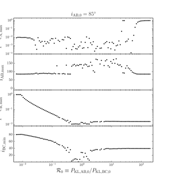
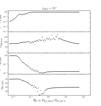
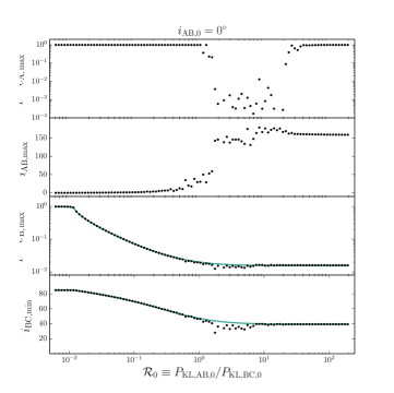
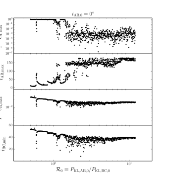
Figure 7: The maximum eccentricities in binaries A and B (first and third panels from the top), the maximum inclination between binaries A and B (second panels from the top), and the minimum inclination between binaries B and C (fourth panels from the top), as a function of the ratio 0subscript0\mathcal{R}_{0} of the KL time-scales for the AB and BC pairs (cf. equation 3.3). Here, 0subscript0\mathcal{R}_{0} is varied by changing the initial aAsubscript𝑎Aa_{\mathrm{A}} and keeping the other initial semimajor axes, masses and eccentricities fixed. In both left- and right-hand panels, the initial conditions are the same as in Section 3.1 and Section 3.2, i.e. semimajor axes aB=102AUsubscript𝑎Bsuperscript102AUa_{\mathrm{B}}=10^{2}\,\mathrm{AU} and aC=5×10³AUsubscript𝑎C5superscript103AUa_{\mathrm{C}}=5\times 10^{3}\,\mathrm{AU}, masses m1=m3=m4=1Msubscript𝑚1subscript𝑚3subscript𝑚41subscriptMdirect-productm_{1}=m_{3}=m_{4}=1\,\mathrm{M}_{\odot} and m2=0.5Msubscript𝑚20.5subscriptMdirect-productm_{2}=0.5\,\mathrm{M}_{\odot}, eccentricities eA=eB=eC=0.01subscript𝑒Asubscript𝑒Bsubscript𝑒C0.01e_{\mathrm{A}}=e_{\mathrm{B}}=e_{\mathrm{C}}=0.01, arguments of pericentre ωA=ωB=ωC=0subscript𝜔Asubscript𝜔Bsubscript𝜔Csuperscript0\omega_{\mathrm{A}}=\omega_{\mathrm{B}}=\omega_{\mathrm{C}}=0^{\circ} and longitudes of the ascending nodes ΩA=ΩB=ΩC=0subscriptΩAsubscriptΩBsubscriptΩCsuperscript0\Omega_{\mathrm{A}}=\Omega_{\mathrm{B}}=\Omega_{\mathrm{C}}=0^{\circ}. In the left- (right-hand) panels, binaries A and B are assumed to be initially coplanar (inclined by 85superscript8585^{\circ}), i.e. in the left-hand panel, iA=iB=0subscript𝑖Asubscript𝑖Bsuperscript0i_{\mathrm{A}}=i_{\mathrm{B}}=0^{\circ} and iC=85subscript𝑖Csuperscript85i_{\mathrm{C}}=85^{\circ}, whereas in the right-hand panel, iA=iC=85subscript𝑖Asubscript𝑖Csuperscript85i_{\mathrm{A}}=i_{\mathrm{C}}=85^{\circ} and iB=0subscript𝑖Bsuperscript0i_{\mathrm{B}}=0^{\circ}. Black dots: computed with SecularQuadruple (the integration time was 20PKL,BC20subscript𝑃KLBC20\,P_{\mathrm{KL,BC}}); solid lines: computed using the semianalytic method discussed in Section 3.4.2.

3.4 Quantitative dependence on 0subscript0\mathcal{R}_{0}

3.4.1 Results from numerical integrations

Here, we describe the dynamics outlined in Section 3.3 more quantitatively, focusing in particular on the effect of the quenching of KL eccentricity oscillations in binary B by the induced precession of binary A, and on the excitation of the eccentricity in binary A in the regime 01similar-tosubscript01\mathcal{R}_{0}\sim 1.

In Fig. 7, we show with black dots the maximum eccentricities in binaries A and B, the maximum inclination between binaries A and B, and the minimum inclination between binaries B and C as a function of 0subscript0\mathcal{R}_{0}, as determined from numerical integrations with SecularQuadruple. Here, 0subscript0\mathcal{R}_{0} is varied by changing aAsubscript𝑎Aa_{\mathrm{A}} (cf. equation 3.3) in the sequence of integrations described in the beginning of Section 3. In the left (right) panels, results are shown assuming that binaries A and B are initially coplaner (highly inclined).
For iAB,0=0subscript𝑖AB0superscript0i_{\mathrm{AB,0}}=0^{\circ}, iAB,maxsubscript𝑖ABmaxi_{\mathrm{AB,max}} is zero for 01less-than-or-similar-tosubscript01\mathcal{R}_{0}\lesssim 1 and rapidly increases for 01greater-than-or-equivalent-tosubscript01\mathcal{R}_{0}\gtrsim 1; eA,maxsubscript𝑒Amaxe_{\mathrm{A,max}} is equal to the initial value for 01less-than-or-similar-tosubscript01\mathcal{R}_{0}\lesssim 1 and for 020greater-than-or-equivalent-tosubscript020\mathcal{R}_{0}\gtrsim 20. This is consistent with the trend that was outlined in Section 3.3. Furthermore, if 0102less-than-or-similar-tosubscript0superscript102\mathcal{R}_{0}\lesssim 10^{-2}, eB,max0subscript𝑒Bmax0e_{\mathrm{B,max}}\approx 0, demonstrating that the induced precession of system A on B in this regime can completely quench any KL oscillations in binary B. Consequently, the minimum inclination between binaries B and C is constant and 85absentsuperscript85\approx 85^{\circ}, the initial value (note that for the regular KL oscillations in binary B, a maximum eccentricity corresponds to minimum inclination with respect to binary C). If 1020less-than-or-similar-to1subscript0less-than-or-similar-to201\lesssim\mathcal{R}_{0}\lesssim 20, iAB,maxsubscript𝑖ABmaxi_{\mathrm{AB,max}} is non-zero; eA,maxsubscript𝑒Amaxe_{\mathrm{A,max}} is also non-zero and reaches high values of up to 1104absent1superscript104\approx 1-10^{-4}. Although the behaviour of these two quantities as a function of 0subscript0\mathcal{R}_{0} is non-regular, there is a general trend in which iAB,maxsubscript𝑖ABmaxi_{\mathrm{AB,max}} asymptotes to 160absentsuperscript160\approx 160^{\circ}. A general trend is also apparent in eA,maxsubscript𝑒Amaxe_{\mathrm{A,max}}.

If binaries A and B are initially inclined by 85superscript8585^{\circ} (cf. the right-hand panels in Fig. 7), the dependence of eA,maxsubscript𝑒Amaxe_{\mathrm{A,max}} as a function of 0subscript0\mathcal{R}_{0} is more complicated. For a large range in 0subscript0\mathcal{R}_{0}, 3×102050less-than-or-similar-to3superscript102subscript0less-than-or-similar-to503\times 10^{-2}\lesssim\mathcal{R}_{0}\lesssim 50, eA,maxsubscript𝑒Amaxe_{\mathrm{A,max}} fluctuates strongly with 0subscript0\mathcal{R}_{0}, reaching high values of 1eA,max104similar-to1subscript𝑒Amaxsuperscript1041-e_{\mathrm{A,max}}\sim 10^{-4} for 0subscript0\mathcal{R}_{0} already as low as 03×102subscript03superscript102\mathcal{R}_{0}\approx 3\times 10^{-2}. For 050greater-than-or-equivalent-tosubscript050\mathcal{R}_{0}\gtrsim 50, eA,maxsubscript𝑒Amaxe_{\mathrm{A,max}} approaches eA,0subscript𝑒A0e_{\mathrm{A,0}}, as was observed previously in Section 3.2. Furthermore, binary B is more affected compared to the coplanar case, in the sense that iBC,minsubscript𝑖BCmini_{\mathrm{BC,min}} decreases more strongly in the regime 1020less-than-or-similar-to1subscript0less-than-or-similar-to201\lesssim\mathcal{R}_{0}\lesssim 20. The maximum eccentricity in binary B is similar to the coplanar case, however.

3.4.2 Semianalytic description

The maximum eccentricity (and hence minimum inclination) reached in binary B can be computed approximately using a semianalytic method based on conservation of the total energy (i.e. the Hamiltonian) and the total angular momentum. This method is similar to that used by Miller & Hamilton (2002); Blaes et al. (2002); Fabrycky & Tremaine (2007); Naoz et al. (2013a). We neglect any changes in binary A between the initial and final states, where the final state corresponds to a maximum eccentricity in binary B. To our knowledge, it is not possible to predict (i.e. without resorting to ‘brute-force’ numerical integrations as in Section 3.4.1) these changes in system A, and this is likely related to the generally chaotic nature of the evolution of binary A, in particular in the regime 1020less-than-or-similar-to1subscript0less-than-or-similar-to201\lesssim\mathcal{R}_{0}\lesssim 20 (cf. Section 3.5). Stated more mathematically, conservation of total energy and angular momentum and the condition that eBsubscript𝑒Be_{\mathrm{B}} is stationary, do not generally provide enough constraints to solve both for eB,maxsubscript𝑒Bmaxe_{\mathrm{B,max}} and the corresponding eAsubscript𝑒Ae_{\mathrm{A}}.

In the Hamiltonian to quadrupole order and for the hierarchy considered here, the term corresponding to binaries A and C in the Hamiltonian can safely be neglected. This can readily be seen from equation (33b): the three terms at quadrupole order scale with the semimajor axes according to

H¯quad,ABsubscript¯𝐻quadAB\displaystyle\overline{H}_{\mathrm{quad,AB}} 1aB(aAaB)2;H¯quad,BC1aC(aBaC)2;formulae-sequenceproportional-toabsent1subscript𝑎Bsuperscriptsubscript𝑎Asubscript𝑎B2proportional-tosubscript¯𝐻quadBC1subscript𝑎Csuperscriptsubscript𝑎Bsubscript𝑎C2\displaystyle\propto\frac{1}{a_{\mathrm{B}}}\left(\frac{a_{\mathrm{A}}}{a_{\mathrm{B}}}\right)^{2};\quad\overline{H}_{\mathrm{quad,BC}}\propto\frac{1}{a_{\mathrm{C}}}\left(\frac{a_{\mathrm{B}}}{a_{\mathrm{C}}}\right)^{2};
H¯quad,ACsubscript¯𝐻quadAC\displaystyle\overline{H}_{\mathrm{quad,AC}} 1aC(aAaC)2.proportional-toabsent1subscript𝑎Csuperscriptsubscript𝑎Asubscript𝑎C2\displaystyle\propto\frac{1}{a_{\mathrm{C}}}\left(\frac{a_{\mathrm{A}}}{a_{\mathrm{C}}}\right)^{2}. (14)

Because, by assumption, aCaBaAmuch-greater-thansubscript𝑎Csubscript𝑎Bmuch-greater-thansubscript𝑎Aa_{\mathrm{C}}\gg a_{\mathrm{B}}\gg a_{\mathrm{A}}, this implies that H¯quad,ACsubscript¯𝐻quadAC\overline{H}_{\mathrm{quad,AC}} can be neglected compared to H¯quad,ABsubscript¯𝐻quadAB\overline{H}_{\mathrm{quad,AB}} and H¯quad,BCsubscript¯𝐻quadBC\overline{H}_{\mathrm{quad,BC}}. The Hamiltonian to quadrupole order is therefore well approximated by (cf. equation 33b)

H¯0subscript¯𝐻0\displaystyle\overline{H}_{0} =CABjB5[(16eA2)jB2+15(𝒆A𝒋B)23(𝒋A𝒋B)2]absentsubscript𝐶ABsuperscriptsubscript𝑗B5delimited-[]16superscriptsubscript𝑒A2superscriptsubscript𝑗B215superscriptsubscript𝒆Asubscript𝒋B23superscriptsubscript𝒋Asubscript𝒋B2\displaystyle=C_{\mathrm{AB}}j_{\mathrm{B}}^{-5}\left[\left(1-6e_{\mathrm{A}}^{2}\right)j_{\mathrm{B}}^{2}+15\left(\boldsymbol{e}_{\mathrm{A}}\cdot\boldsymbol{j}_{\mathrm{B}}\right)^{2}-3\left(\boldsymbol{j}_{\mathrm{A}}\cdot\boldsymbol{j}_{\mathrm{B}}\right)^{2}\right]
+CBCjC5[(16eB2)jC2+15(𝒆B𝒋C)23(𝒋B𝒋C)2],subscript𝐶BCsuperscriptsubscript𝑗C5delimited-[]16superscriptsubscript𝑒B2superscriptsubscript𝑗C215superscriptsubscript𝒆Bsubscript𝒋C23superscriptsubscript𝒋Bsubscript𝒋C2\displaystyle+C_{\mathrm{BC}}j_{\mathrm{C}}^{-5}\left[\left(1-6e_{\mathrm{B}}^{2}\right)j_{\mathrm{C}}^{2}+15\left(\boldsymbol{e}_{\mathrm{B}}\cdot\boldsymbol{j}_{\mathrm{C}}\right)^{2}-3\left(\boldsymbol{j}_{\mathrm{B}}\cdot\boldsymbol{j}_{\mathrm{C}}\right)^{2}\right], (15)

where

CABsubscript𝐶AB\displaystyle C_{\mathrm{AB}} =18Gm1m2m3m1+m21aB(aAaB)2;absent18𝐺subscript𝑚1subscript𝑚2subscript𝑚3subscript𝑚1subscript𝑚21subscript𝑎Bsuperscriptsubscript𝑎Asubscript𝑎B2\displaystyle=\frac{1}{8}\frac{Gm_{1}m_{2}m_{3}}{m_{1}+m_{2}}\frac{1}{a_{\mathrm{B}}}\left(\frac{a_{\mathrm{A}}}{a_{\mathrm{B}}}\right)^{2};
CBCsubscript𝐶BC\displaystyle C_{\mathrm{BC}} =18G(m1+m2)m3m4m1+m2+m31aC(aBaC)2.absent18𝐺subscript𝑚1subscript𝑚2subscript𝑚3subscript𝑚4subscript𝑚1subscript𝑚2subscript𝑚31subscript𝑎Csuperscriptsubscript𝑎Bsubscript𝑎C2\displaystyle=\frac{1}{8}\frac{G(m_{1}+m_{2})m_{3}m_{4}}{m_{1}+m_{2}+m_{3}}\frac{1}{a_{\mathrm{C}}}\left(\frac{a_{\mathrm{B}}}{a_{\mathrm{C}}}\right)^{2}. (16)

The equation of motion for 𝒆Bsubscript𝒆B\boldsymbol{e}_{\mathrm{B}} that follows from equation (3.4.2) is given by (cf. equation 4)

d𝒆Bdt=6ΛBdsubscript𝒆Bd𝑡6subscriptΛB\displaystyle\frac{\mathrm{d}\boldsymbol{e}_{\mathrm{B}}}{\mathrm{d}t}=\frac{6}{\Lambda_{\mathrm{B}}}
×[CABjB5{(𝒋A𝒋B)(𝒆B×𝒋A)+5(𝒆A𝒋B)(𝒆A×𝒆B)}\displaystyle\quad\times\left[C_{\mathrm{AB}}j_{\mathrm{B}}^{-5}\left\{\left(\boldsymbol{j}_{\mathrm{A}}\cdot\boldsymbol{j}_{\mathrm{B}}\right)\left(\boldsymbol{e}_{\mathrm{B}}\times\boldsymbol{j}_{\mathrm{A}}\right)+5\left(\boldsymbol{e}_{\mathrm{A}}\cdot\boldsymbol{j}_{\mathrm{B}}\right)\left(\boldsymbol{e}_{\mathrm{A}}\times\boldsymbol{e}_{\mathrm{B}}\right)\right\}\right.
+CBCjC5{(𝒋B𝒋C)(𝒆B×𝒋C)5(𝒆B𝒋C)(𝒋B×𝒋C)}].\displaystyle\quad\quad\left.+C_{\mathrm{BC}}j_{\mathrm{C}}^{-5}\left\{\left(\boldsymbol{j}_{\mathrm{B}}\cdot\boldsymbol{j}_{\mathrm{C}}\right)\left(\boldsymbol{e}_{\mathrm{B}}\times\boldsymbol{j}_{\mathrm{C}}\right)-5\left(\boldsymbol{e}_{\mathrm{B}}\cdot\boldsymbol{j}_{\mathrm{C}}\right)\left(\boldsymbol{j}_{\mathrm{B}}\times\boldsymbol{j}_{\mathrm{C}}\right)\right\}\right].

A stationary value of eBsubscript𝑒Be_{\mathrm{B}} corresponds to

0=deBdt=𝒆^Bd𝒆Bdt.0dsubscript𝑒Bd𝑡subscript^𝒆Bdsubscript𝒆Bd𝑡\displaystyle 0=\frac{\mathrm{d}e_{\mathrm{B}}}{\mathrm{d}t}=\hat{\boldsymbol{e}}_{\mathrm{B}}\cdot\frac{\mathrm{d}\boldsymbol{e}_{\mathrm{B}}}{\mathrm{d}t}. (17)

Neglecting the terms proportional to CABsubscript𝐶ABC_{\mathrm{AB}} in equation (3.4.2), this condition implies 𝒆B𝒋C=0subscript𝒆Bsubscript𝒋C0\boldsymbol{e}_{\mathrm{B}}\cdot\boldsymbol{j}_{\mathrm{C}}=0, and/or (𝒋B×𝒋C)𝒆B=0subscript𝒋Bsubscript𝒋Csubscript𝒆B0(\boldsymbol{j}_{\mathrm{B}}\times\boldsymbol{j}_{\mathrm{C}})\cdot\boldsymbol{e}_{\mathrm{B}}=0. The former cannot be generally true in the case of a maximum eccentricity, therefore the second condition must apply. The latter can be rewritten using the vector identity equation (37) as

(𝒆^B𝒋^C)2=1(𝒋^B𝒋^C)2.superscriptsubscript^𝒆Bsubscript^𝒋C21superscriptsubscript^𝒋Bsubscript^𝒋C2\displaystyle\left(\hat{\boldsymbol{e}}_{\mathrm{B}}\cdot\hat{\boldsymbol{j}}_{\mathrm{C}}\right)^{2}=1-\left(\hat{\boldsymbol{j}}_{\mathrm{B}}\cdot\hat{\boldsymbol{j}}_{\mathrm{C}}\right)^{2}. (18)

The mutual inclination between binaries B and C can be related to eBsubscript𝑒Be_{\mathrm{B}} using conservation of the total angular momentum vector,

𝑳tot=ΛA𝒋A+ΛB𝒋B+ΛC𝒋C.subscript𝑳totsubscriptΛAsubscript𝒋AsubscriptΛBsubscript𝒋BsubscriptΛCsubscript𝒋C\displaystyle\boldsymbol{L}_{\mathrm{tot}}=\Lambda_{\mathrm{A}}\boldsymbol{j}_{\mathrm{A}}+\Lambda_{\mathrm{B}}\boldsymbol{j}_{\mathrm{B}}+\Lambda_{\mathrm{C}}\boldsymbol{j}_{\mathrm{C}}. (19)

At this level of approximation,

𝒆CH¯0=𝟎,subscriptsubscript𝒆Csubscript¯𝐻00\displaystyle\nabla_{\boldsymbol{e}_{\mathrm{C}}}\overline{H}_{0}=\boldsymbol{0}, (20)

therefore

deCdt=𝒆^Cd𝒆Cdt=1ΛC[𝒆^C(𝒆C×𝒋CH¯0)]=0,dsubscript𝑒Cd𝑡subscript^𝒆Cdsubscript𝒆Cd𝑡1subscriptΛCdelimited-[]subscript^𝒆Csubscript𝒆Csubscriptsubscript𝒋Csubscript¯𝐻00\displaystyle\frac{\mathrm{d}e_{\mathrm{C}}}{\mathrm{d}t}=\hat{\boldsymbol{e}}_{\mathrm{C}}\cdot\frac{\mathrm{d}\boldsymbol{e}_{\mathrm{C}}}{\mathrm{d}t}=-\frac{1}{\Lambda_{\mathrm{C}}}\left[\hat{\boldsymbol{e}}_{\mathrm{C}}\cdot\left(\boldsymbol{e}_{\mathrm{C}}\times\nabla_{\boldsymbol{j}_{\mathrm{C}}}\overline{H}_{0}\right)\right]=0, (21)

and eCsubscript𝑒Ce_{\mathrm{C}} is constant. Neglecting the term corresponding to binary A and writing eC=eC,0subscript𝑒Csubscript𝑒C0e_{\mathrm{C}}=e_{\mathrm{C,0}}, equation (19) gives

𝒋^B𝒋^Csubscript^𝒋Bsubscript^𝒋C\displaystyle\hat{\boldsymbol{j}}_{\mathrm{B}}\cdot\hat{\boldsymbol{j}}_{\mathrm{C}} =121eB21eC,02[21eB,021eC,02\displaystyle=\frac{1}{2\sqrt{1-e_{\mathrm{B}}^{2}}\sqrt{1-e_{\mathrm{C,0}}^{2}}}\left[2\sqrt{1-e_{\mathrm{B,0}}^{2}}\sqrt{1-e_{\mathrm{C,0}}^{2}}\right.
×(𝒋^B𝒋^C)0+ΛBΛC(eB2eB,02)].\displaystyle\quad\times\left.\left(\hat{\boldsymbol{j}}_{\mathrm{B}}\cdot\hat{\boldsymbol{j}}_{\mathrm{C}}\right)_{0}+\frac{\Lambda_{\mathrm{B}}}{\Lambda_{\mathrm{C}}}\left(e_{\mathrm{B}}^{2}-e_{\mathrm{B,0}}^{2}\right)\right]. (22)

Furthermore, if any changes in binary A between the initial and final state are neglected, then the remaining unknown terms in equation (3.4.2) are simply given by eA=eA,0subscript𝑒Asubscript𝑒A0e_{\mathrm{A}}=e_{\mathrm{A,0}}, 𝒋A𝒋B=(𝒋A𝒋B)0subscript𝒋Asubscript𝒋Bsubscriptsubscript𝒋Asubscript𝒋B0\boldsymbol{j}_{\mathrm{A}}\cdot\boldsymbol{j}_{\mathrm{B}}=(\boldsymbol{j}_{\mathrm{A}}\cdot\boldsymbol{j}_{\mathrm{B}})_{0} and 𝒆A𝒋B=(𝒆A𝒋B)0subscript𝒆Asubscript𝒋Bsubscriptsubscript𝒆Asubscript𝒋B0\boldsymbol{e}_{\mathrm{A}}\cdot\boldsymbol{j}_{\mathrm{B}}=(\boldsymbol{e}_{\mathrm{A}}\cdot\boldsymbol{j}_{\mathrm{B}})_{0}.

With these simplifications, equation (3.4.2) only contains the single unknown quantity eBsubscript𝑒Be_{\mathrm{B}} corresponding to stationary points. In general, this equation cannot be solved analytically. A notable exception is when the term proportional to CABsubscript𝐶ABC_{\mathrm{AB}} in equation (3.4.2) is neglected (i.e. neglecting the contribution from binary A), as is the term proportional to ΛB/ΛCsubscriptΛBsubscriptΛC\Lambda_{\mathrm{B}}/\Lambda_{\mathrm{C}} in equation (22) (i.e. assuming a highly hierarchical system). In that case, the solution corresponding to the maximum eccentricity is

eB,max=153(𝒋^B𝒋^C)02,subscript𝑒Bmax153superscriptsubscriptsubscript^𝒋Bsubscript^𝒋C02\displaystyle e_{\mathrm{B,max}}=\sqrt{1-\frac{5}{3}\left(\hat{\boldsymbol{j}}_{\mathrm{B}}\cdot\hat{\boldsymbol{j}}_{\mathrm{C}}\right)_{0}^{2}}, (23)

which is a well-known result for hierarchical triple systems applied to binaries B and C, and where binary A is essentially replaced by a point mass (note that 𝒋^B𝒋^C=cos[iBC]subscript^𝒋Bsubscript^𝒋Csubscript𝑖BC\hat{\boldsymbol{j}}_{\mathrm{B}}\cdot\hat{\boldsymbol{j}}_{\mathrm{C}}=\cos[i_{\mathrm{BC}}]). More general numerical solutions are shown in the bottom two panels of Fig. 7 with the solid lines, where iBC,minsubscript𝑖BCmini_{\mathrm{BC,min}} is computed using equation (22). Although the semianalytic curves do not capture the detailed behaviour of eB,maxsubscript𝑒Bmaxe_{\mathrm{B,max}} and iBC,minsubscript𝑖BCmini_{\mathrm{BC,min}} in the regime 1020less-than-or-similar-to1subscript0less-than-or-similar-to201\lesssim\mathcal{R}_{0}\lesssim 20, for other 0subscript0\mathcal{R}_{0} they agree well with the results obtained from the numerical integrations with SecularQuadruple.
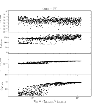
Refer to caption
Refer to caption
Figure 8: Similar to Fig. 7, showing greater detail near 0=1subscript01\mathcal{R}_{0}=1.

3.5 Behaviour near 0=1subscript01\mathcal{R}_{0}=1

It is apparent from Fig. 7 that near 0=1subscript01\mathcal{R}_{0}=1, the behaviour of the maximum eccentricities of binaries A and B as a function of 0subscript0\mathcal{R}_{0} is complex and non-regular. Here, we briefly discuss in more detail the behaviour in this regime based on numerical integrations with SecularQuadruple.

In Fig. 8, we show the same quantities as in Fig. 7, now based on 1000 numerical integrations within a smaller interval of 0subscript0\mathcal{R}_{0} near 0=1subscript01\mathcal{R}_{0}=1. In the coplanar case and for 01less-than-or-similar-tosubscript01\mathcal{R}_{0}\lesssim 1, there are distinct peaks corresponding to enhanced eccentricities in both binaries A and B at specific values of 0subscript0\mathcal{R}_{0}. For 01greater-than-or-equivalent-tosubscript01\mathcal{R}_{0}\gtrsim 1, individual peaks are harder to distinguish. We speculate that the peaked behaviour is due to resonances in the arguments of pericentre of binaries A and B that occur at specific integer ratios of the KL time-scales for the AB and BC pairs. In addition, for 01greater-than-or-equivalent-tosubscript01\mathcal{R}_{0}\gtrsim 1 there may be an overlap of many resonances, thereby producing a chaotic behaviour as a function of 0subscript0\mathcal{R}_{0} (Chirikov, 1979). Interestingly, the peaks for 01less-than-or-similar-tosubscript01\mathcal{R}_{0}\lesssim 1 are much less pronounced, if not completely absent, in the highly inclined case.

These phenomena merit further study, but are beyond the scope of this work.

3.6 General relativistic effects
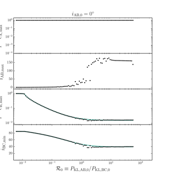
Refer to caption
Refer to caption
Figure 9: Similar to Fig. 7, but here with the inclusion of relativistic precession to 1PN order in all three binary systems.

In the results presented above, all four bodies were assumed to be point masses and general relativistic effects were not included. In Fig. 9, we show the results of integrations with SecularQuadruple similar to those presented in Fig. 7, but now including 1PN precession in the equations of motion for all three binaries (cf. equation 9). We note that in the sequence of integrations shown in the left- and right-hand panels of Fig. 9, only aAsubscript𝑎Aa_{\mathrm{A}} is varied; consequently, both t1PN,Asubscript𝑡1PNAt_{\mathrm{1PN,A}} (cf. equation 8) and PKL,ABsubscript𝑃KLABP_{\mathrm{KL,AB}} (cf. equation 11) are affected. For the smallest value of 0subscript0\mathcal{R}_{0} in Fig. 9 (largest value of aA=1AUsubscript𝑎A1AUa_{\mathrm{A}}=1\,\mathrm{AU}, cf. panels 1-6 in Figs 5 and 6), the initial t1PN,A18.4Myrsubscript𝑡1PNA18.4Myrt_{\mathrm{1PN,A}}\approx 18.4\,\mathrm{Myr} and PKL,AB1.2Myrsubscript𝑃KLAB1.2MyrP_{\mathrm{KL,AB}}\approx 1.2\,\mathrm{Myr}. For the largest value of 0subscript0\mathcal{R}_{0} in Fig. 9 (smallest value of aA=0.001AUsubscript𝑎A0.001AUa_{\mathrm{A}}=0.001\,\mathrm{AU}, cf. panels 7-12 in Figs 5 and 6), the initial t1PN,A5.8×107Myrsubscript𝑡1PNA5.8superscript107Myrt_{\mathrm{1PN,A}}\approx 5.8\times 10^{-7}\,\mathrm{Myr} and PKL,AB3.9×104Myrsubscript𝑃KLAB3.9superscript104MyrP_{\mathrm{KL,AB}}\approx 3.9\times 10^{4}\,\mathrm{Myr}.

In the coplanar case, eccentricity oscillations in binary A are quenched due to relativistic precession, even if 01similar-tosubscript01\mathcal{R}_{0}\sim 1. We note, however, that the purely Newtonian results can be rescaled to other systems (in particular, with larger aAsubscript𝑎Aa_{\mathrm{A}}), in which case relativistic precession in binary A becomes unimportant, whereas the purely Newtonian secular dynamics remain unaffected modulo a rescaling of the KL time-scales.

In the inclined case, the behaviour of the maximum eccentricity in binary A is more complicated (cf. the right-hand panel of Fig. 9). For the lowest 0subscript0\mathcal{R}_{0}, PKL,AB<t1PN,Asubscript𝑃KLABsubscript𝑡1PNAP_{\mathrm{KL,AB}}<t_{\mathrm{1PN,A}} as mentioned above. As 0subscript0\mathcal{R}_{0} is increased, the quantity eA,maxsubscript𝑒Amaxe_{\mathrm{A,max}} decreases with increasing 0subscript0\mathcal{R}_{0}, which is due to the increasing relative importance of 1PN precession compared to the torque of binary B. However, the decrease of eA,maxsubscript𝑒Amaxe_{\mathrm{A,max}} flattens around 02×102subscript02superscript102\mathcal{R}_{0}\approx 2\times 10^{-2}. The latter value of 0subscript0\mathcal{R}_{0} corresponds to a significant increase of eB,maxsubscript𝑒Bmaxe_{\mathrm{B,max}}. The flattening of eA,maxsubscript𝑒Amaxe_{\mathrm{A,max}} as a function of 0subscript0\mathcal{R}_{0} can be explained by considering that as eB,maxsubscript𝑒Bmaxe_{\mathrm{B,max}} increases, the KL time-scale for the AB pair decreases (cf. equation 11). Consequently, the latter KL time-scale can become comparable to the 1PN precession time-scale. Here, this is the case for 2×1020101less-than-or-similar-to2superscript102subscript0less-than-or-similar-tosuperscript1012\times 10^{-2}\lesssim\mathcal{R}_{0}\lesssim 10^{-1}.

We show an example of this phenomenon in Fig. 10, where aA0.3AUsubscript𝑎A0.3AUa_{\mathrm{A}}\approx 0.3\,\mathrm{AU} and 00.04subscript00.04\mathcal{R}_{0}\approx 0.04 (full parameters are given in the caption). At the maxima of eBsubscript𝑒Be_{\mathrm{B}}, the KL time-scale for the AB binary pair (black solid line in the top-left panel) decreases and becomes comparable to the 1PN precession time-scale in binary A (red solid line in the same panel). This gives rise to increased eccentricities in binary A, to much higher values if eBsubscript𝑒Be_{\mathrm{B}} were constant (cf. the top-middle panel). This is a mechanism for – at least partially – overcoming the well-known quenching of KL eccentricity cycles induced by 1PN precession. Note, however, that in this case, there is only a narrow region in 0subscript0\mathcal{R}_{0} for which it is effective: as 0subscript0\mathcal{R}_{0} increases, aAsubscript𝑎Aa_{\mathrm{A}} decreases, therefore further decreasing t1PN,Asubscript𝑡1PNAt_{\mathrm{1PN,A}}.

We note that this phenomenon is general, in the sense that it would also apply if precession in binary A is due to another effect, e.g. tidal effects or mass transfer in stellar systems.
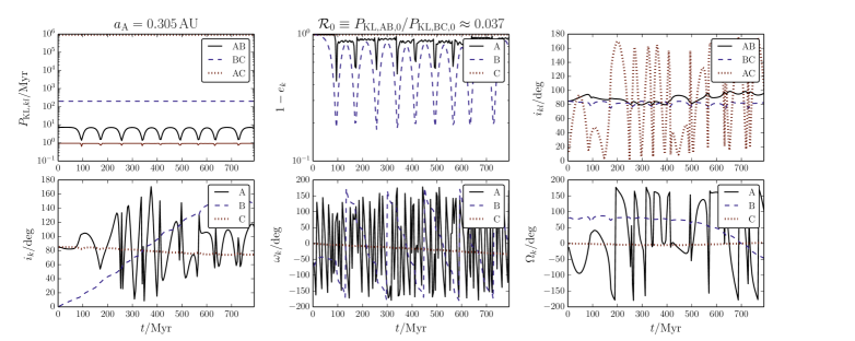
Refer to caption
Figure 10: Evolution for a system taken from Fig. 9, demonstrating the effect of ‘overcoming’ 1PN precession by the periodically enhanced eccentricity of system B. The assumed initial parameters are semimajor axes aB=0.305AUsubscript𝑎B0.305AUa_{\mathrm{B}}=0.305\,\mathrm{AU}, aB=102AUsubscript𝑎Bsuperscript102AUa_{\mathrm{B}}=10^{2}\,\mathrm{AU} and aC=5×10³AUsubscript𝑎C5superscript103AUa_{\mathrm{C}}=5\times 10^{3}\,\mathrm{AU}, masses m1=m3=m4=1Msubscript𝑚1subscript𝑚3subscript𝑚41subscriptMdirect-productm_{1}=m_{3}=m_{4}=1\,\mathrm{M}_{\odot} and m2=0.5Msubscript𝑚20.5subscriptMdirect-productm_{2}=0.5\,\mathrm{M}_{\odot}, eccentricities eA=eB=eC=0.01subscript𝑒Asubscript𝑒Bsubscript𝑒C0.01e_{\mathrm{A}}=e_{\mathrm{B}}=e_{\mathrm{C}}=0.01, inclinations iA=iC=85subscript𝑖Asubscript𝑖Csuperscript85i_{\mathrm{A}}=i_{\mathrm{C}}=85^{\circ} and iB=0subscript𝑖Bsuperscript0i_{\mathrm{B}}=0^{\circ}, arguments of pericentre ωA=ωB=ωC=0subscript𝜔Asubscript𝜔Bsubscript𝜔Csuperscript0\omega_{\mathrm{A}}=\omega_{\mathrm{B}}=\omega_{\mathrm{C}}=0^{\circ} and longitudes of the ascending nodes ΩA=ΩB=ΩC=0subscriptΩAsubscriptΩBsubscriptΩCsuperscript0\Omega_{\mathrm{A}}=\Omega_{\mathrm{B}}=\Omega_{\mathrm{C}}=0^{\circ}. In the top-left panel, the solid red line shows the 1PN precession time-scale in binary A (cf. equation 8).

4 Discussion

4.1 Application: planetary systems

As mentioned in Section 1, the hierarchical configuration considered in this work can be applied to planetary systems consisting of a planet+moon system (binary A) orbiting a central star (in binary B) that is orbited by a more distant and inclined planetary or stellar companion (in binary C). Both binaries A and B are assumed to be initially coplanar and circular. A pertinent question is whether the torque exerted by the fourth body causes the planet+moon system to become inclined with respect to the orbit of the central star, or whether coplanarity is maintained. We note that this is different from the question that has been addressed in the past in which case a different hierarchy was assumed, i.e. all bodies within the stellar binary were assumed to orbit the central star (Innanen et al., 1997; Takeda & Rasio, 2005; Takeda et al., 2008).

Based on the qualitative results presented in Section 3.3, we expect that coplanarity between binaries A and B is maintained if PKL,AB,0PKL,BC,0much-less-thansubscript𝑃KLAB0subscript𝑃KLBC0P_{\mathrm{KL,AB,0}}\ll P_{\mathrm{KL,BC,0}}, i.e. if the binary companion is distant from the planetary orbit. In addition, we expect KL eccentricity oscillations in the orbit of the planet+moon system with respect to the central star due to the torque of the binary companion to be quenched. This effect could prevent the latter orbit from becoming highly eccentric, i.e. the presence of the moon could ‘shield’ the planet from disruption by the star as a consequence of KL oscillations induced by the binary companion.

On the other hand, if PKL,AB,0PKL,BC,0much-greater-thansubscript𝑃KLAB0subscript𝑃KLBC0P_{\mathrm{KL,AB,0}}\gg P_{\mathrm{KL,BC,0}}, the binary companion is close to the planetary orbit, and the planet+moon system can become inclined with respect to the orbit of the central star. However, in the latter case, the KL time-scale for the AB pair is long compared to that of the BC pair, such that there is no eccentricity excitation in the planet+moon system. In the intermediate regime where PKL,AB,0PKL,BC,0similar-tosubscript𝑃KLAB0subscript𝑃KLBC0P_{\mathrm{KL,AB,0}}\sim P_{\mathrm{KL,BC,0}}, we expect significant eccentricity oscillations in the planet+moon system. These oscillations could lead to efficient tidal dissipation in cases where this would otherwise not have been important, and, in extreme cases, even to planet+moon collisions.

We explore in Section 4.1.1 some of the parameter space where significant KL eccentricity oscillations in the planet+moon system are expected, and give a number of examples in Section 4.1.2. A comprehensive population synthesis study is beyond the scope of this paper.
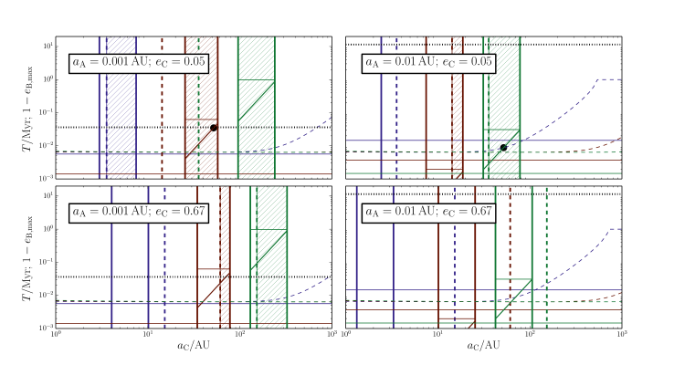
Refer to caption
Figure 11: Exploration of the parameter space where eccentricity oscillations could be induced in a planet+moon system orbiting a central star that is orbited by an inclined binary companion (cf. Section 4.1). Blue, red and green lines correspond to semimajor axes aBsubscript𝑎Ba_{\mathrm{B}} of the planet+moon system with respect to the central star of 1, 4 and 10 AU, respectively. The ranges of aCsubscript𝑎Ca_{\mathrm{C}} for which 1<0<201subscript0201<\mathcal{R}_{0}<20 are indicated with vertical thick coloured solid lines. Values of aCsubscript𝑎Ca_{\mathrm{C}} corresponding to dynamical stability of the BC pair (according to the criterion of Mardling & Aarseth 2001) are indicated with vertical thick coloured dashed lines. The regions where we expect that the eccentricity of the planet+moon system is excited, are indicated with hatches. Near the hatches regions, the horizontal solid lines show PKL,AB,0subscript𝑃KLAB0P_{\mathrm{KL,AB,0}}, whereas the sloped solid lines show PKL,BC,0subscript𝑃KLBC0P_{\mathrm{KL,BC,0}}. The black horizontal dotted lines indicate the time-scale for relativistic precession in binary A. In addition to these time-scales, we show with non-vertical coloured dashed lines the maximum eccentricity in binary B, computed using the method of Section 3.4.2, and assuming iBC,0=85subscript𝑖BC0superscript85i_{\mathrm{BC,0}}=85^{\circ}. The horizontal coloured solid lines show the value of 1eB1subscript𝑒B1-e_{\mathrm{B}} for which the planet+moon system is expected to be disrupted by the central star. In the top two panels, the black bullets correspond to the two example systems discussed in Section 4.1.2.
Refer to caption
Refer to caption
Figure 12: Evolution of two quadruple systems in the context of planetary systems as discussed in Section 4.1.2, computed with SecularQuadruple. First two rows: aA=103AUsubscript𝑎Asuperscript103AUa_{\mathrm{A}}=10^{-3}\,\mathrm{AU}, aB=4AUsubscript𝑎B4AUa_{\mathrm{B}}=4\,\mathrm{AU} and aC=50AUsubscript𝑎C50AUa_{\mathrm{C}}=50\,\mathrm{AU}; second two rows: aA=102AUsubscript𝑎Asuperscript102AUa_{\mathrm{A}}=10^{-2}\,\mathrm{AU}, aB=10AUsubscript𝑎B10AUa_{\mathrm{B}}=10\,\mathrm{AU} and aC=50AUsubscript𝑎C50AUa_{\mathrm{C}}=50\,\mathrm{AU}. Binaries A and B are initially coplanar, whereas iBC,0=70subscript𝑖BC0superscript70i_{\mathrm{BC,0}}=70^{\circ}. In both examples, the other initial parameters were m1=1MJsubscript𝑚11subscriptMJm_{1}=1\,\mathrm{M}_{\mathrm{J}}, m2=103MJsubscript𝑚2superscript103subscriptMJm_{2}=10^{-3}\,\mathrm{M}_{\mathrm{J}}, m3=1Msubscript𝑚31subscriptMdirect-productm_{3}=1\,\mathrm{M}_{\odot} and m4=0.5Msubscript𝑚40.5subscriptMdirect-productm_{4}=0.5\,\mathrm{M}_{\odot}, eA=eB=0.001subscript𝑒Asubscript𝑒B0.001e_{\mathrm{A}}=e_{\mathrm{B}}=0.001 and eC=0.05subscript𝑒C0.05e_{\mathrm{C}}=0.05, iA=iB=0subscript𝑖Asubscript𝑖Bsuperscript0i_{\mathrm{A}}=i_{\mathrm{B}}=0^{\circ} and iC=70subscript𝑖Csuperscript70i_{\mathrm{C}}=70^{\circ}, ωA=10subscript𝜔Asuperscript10\omega_{\mathrm{A}}=10^{\circ}, ωB=40subscript𝜔Bsuperscript40\omega_{\mathrm{B}}=40^{\circ} and ωC=90subscript𝜔Csuperscript90\omega_{\mathrm{C}}=90^{\circ} and ΩA=ΩB=ΩC=0subscriptΩAsubscriptΩBsubscriptΩCsuperscript0\Omega_{\mathrm{A}}=\Omega_{\mathrm{B}}=\Omega_{\mathrm{C}}=0^{\circ}. In the panels showing eksubscript𝑒𝑘e_{k}, the horizontal solid red line shows the value of eAsubscript𝑒Ae_{\mathrm{A}} for which the moon collides with its planet. Here, we assumed a planet radius R1=1RJsubscript𝑅11subscript𝑅JR_{1}=1\,R_{\mathrm{J}} and lunar radius R2=102RJsubscript𝑅2superscript102subscript𝑅JR_{2}=10^{-2}\,R_{\mathrm{J}}. The integrations were stopped when eAsubscript𝑒Ae_{\mathrm{A}} reached this value.

4.1.1 Expectations based on time-scale arguments

We assume a Jupiter-mass planet, m1=MJsubscript𝑚1subscript𝑀Jm_{1}=M_{\mathrm{J}}, a moon with mass m2=104m1subscript𝑚2superscript104subscript𝑚1m_{2}=10^{-4}\,m_{1} (the order of magnitude of the mass of Jupiter’s heaviest moons), a central star with mass m3=1Msubscript𝑚31subscriptMdirect-productm_{3}=1\,\mathrm{M}_{\odot}, and a binary companion with mass m4=0.5Msubscript𝑚40.5subscriptMdirect-productm_{4}=0.5\,\mathrm{M}_{\odot}. The radii (of interest when considering collisions) are assumed to be R1=RJsubscript𝑅1subscript𝑅JR_{1}=R_{\mathrm{J}}, R2=102R1subscript𝑅2superscript102subscript𝑅1R_{2}=10^{-2}\,R_{1} and R3=1Rsubscript𝑅31subscriptRdirect-productR_{3}=1\,\mathrm{R}_{\odot}.

The semimajor axis of the planet+moon system is assumed to be either aA=103AUsubscript𝑎Asuperscript103AUa_{\mathrm{A}}=10^{-3}\,\mathrm{AU} or aA=102AUsubscript𝑎Asuperscript102AUa_{\mathrm{A}}=10^{-2}\,\mathrm{AU}; the semimajor axis aBsubscript𝑎Ba_{\mathrm{B}} of the latter system with respect to the central star is either 1, 4 or 10 AU. The eccentricities of binaries A and B are assumed to be eA=eB=0.001subscript𝑒Asubscript𝑒B0.001e_{\mathrm{A}}=e_{\mathrm{B}}=0.001; the eccentricity of the orbit of the binary companion is either eC=0.05subscript𝑒C0.05e_{\mathrm{C}}=0.05 or eC=0.67subscript𝑒C0.67e_{\mathrm{C}}=0.67.

In Fig. 11, we show various time-scales of importance as a function of aCsubscript𝑎Ca_{\mathrm{C}}, where in each panel different values are assumed for aAsubscript𝑎Aa_{\mathrm{A}} and eCsubscript𝑒Ce_{\mathrm{C}}. Quantities pertaining to the three values of aBsubscript𝑎Ba_{\mathrm{B}} are indicated with blue, red and green lines for values of aBsubscript𝑎Ba_{\mathrm{B}} of 1, 4 and 10 AU, respectively. The critical values of aCsubscript𝑎Ca_{\mathrm{C}} corresponding to dynamical stability, computed using the three-body criterion of Mardling & Aarseth (2001) and where binary A is treated as a point mass, are indicated with vertical dashed lines for each value of aBsubscript𝑎Ba_{\mathrm{B}}. Systems to the left of these lines are expected to be dynamically unstable.

Extrapolating our results from Section 3, we expect the region in parameter space in which eAsubscript𝑒Ae_{\mathrm{A}} can be excited (in the absence of relativistic effects and other additional sources of absidal motion), to be approximately 1020less-than-or-similar-to1subscript0less-than-or-similar-to201\lesssim\mathcal{R}_{0}\lesssim 20. The limiting values of aCsubscript𝑎Ca_{\mathrm{C}}, for each value of aBsubscript𝑎Ba_{\mathrm{B}}, are indicated with the vertical solid lines, and between these vertical lines the coloured horizontal (sloped) solid lines indicate the KL time-scales for pair AB (BC). We have indicated with hatched regions the ranges in aCsubscript𝑎Ca_{\mathrm{C}} satisfying 1<0<201subscript0201<\mathcal{R}_{0}<20, and the stability constraint.

In principle, the mechanism for producing high-amplitude oscillations in eAsubscript𝑒Ae_{\mathrm{A}} in the regime 01similar-tosubscript01\mathcal{R}_{0}\sim 1 can be suppressed if KL oscillations in system B are quenched by relativistic precession in binary B. In all cases in Fig. 11, these time-scales are longer than 10 Myr, and therefore, precession in binary B is not important. Relativistic precession in binary A is of greater importance given the small values of aAsubscript𝑎Aa_{\mathrm{A}}; the associated time-scales are indicated in Fig. 11 with black dotted horizontal lines.

Based on Fig. 11, we expect eccentricity excitation in the planet+moon system for specific ranges in aCsubscript𝑎Ca_{\mathrm{C}}. These ranges strongly depend on aAsubscript𝑎Aa_{\mathrm{A}}, aBsubscript𝑎Ba_{\mathrm{B}} and eCsubscript𝑒Ce_{\mathrm{C}}. For small semimajor axes of the planet+moon system, i.e. aA=102AUsubscript𝑎Asuperscript102AUa_{\mathrm{A}}=10^{-2}\,\mathrm{AU}, the criterion of dynamical stability of the orbit of the binary companion does not strongly reduce the parameter space. General relativistic precession is, however, also more important for smaller aAsubscript𝑎Aa_{\mathrm{A}}. Nevertheless, for values of aBsubscript𝑎Ba_{\mathrm{B}} of 4 and 10 AU, the relativistic precession time-scale in binary A is not much shorter than the KL time-scale for the AB pair. In those cases, there could still be high-eccentricity oscillations in binary A because of the reduction of the KL time-scale for the AB pair as a consequence of the eccentricity oscillations in binary B (cf. Section 3.6). This is demonstrated below in the first example in Section 4.1.2.

A larger eccentricity of the binary companion tends to reduce the parameter space of interest. The reason for this decrease is the larger range in aCsubscript𝑎Ca_{\mathrm{C}} for which the system is not dynamically stable.

As discussed in Section 3, for 01much-less-thansubscript01\mathcal{R}_{0}\ll 1, KL eccentricity oscillations in binary B are quenched because of the induced precession from binary A. We have plotted the maximum eccentricity in binary B as a function of aCsubscript𝑎Ca_{\mathrm{C}} in Fig. 11 with dashed lines, computed using the semianalytic method described in Section 3.4.2. Here, we assumed iBC,0=85subscript𝑖BC0superscript85i_{\mathrm{BC,0}}=85^{\circ} to get a rough upper limit of the maximum eccentricity. The quenching effect is very effective for aB=1AUsubscript𝑎B1AUa_{\mathrm{B}}=1\,\mathrm{AU} and aCsubscript𝑎Ca_{\mathrm{C}} larger than a few 100 AU. For large enough aCsubscript𝑎Ca_{\mathrm{C}}, eccentricity oscillations in binary B are completely quenched.

To illustrate the implications of this, we have indicated in Fig. 11 with horizontal coloured lines the values of 1eB1subscript𝑒B1-e_{\mathrm{B}} that satisfy 1eB=(aA+R3)/aB1subscript𝑒Bsubscript𝑎Asubscript𝑅3subscript𝑎B1-e_{\mathrm{B}}=(a_{\mathrm{A}}+R_{3})/a_{\mathrm{B}}, i.e. the eccentricity for which the pericentre distance of the orbit of binary B is equal to aA+R3subscript𝑎Asubscript𝑅3a_{\mathrm{A}}+R_{3}. In the latter case, we expect the planet, the moon, or both, to be disrupted by the central star. For aA=102AUsubscript𝑎Asuperscript102AUa_{\mathrm{A}}=10^{-2}\,\mathrm{AU} and aB=1AUsubscript𝑎B1AUa_{\mathrm{B}}=1\,\mathrm{AU}, the maximum eccentricity reached in binary B exceeds this value for aC100AUless-than-or-similar-tosubscript𝑎C100AUa_{\mathrm{C}}\lesssim 100\,\mathrm{AU}. However, for aC100AUgreater-than-or-equivalent-tosubscript𝑎C100AUa_{\mathrm{C}}\gtrsim 100\,\mathrm{AU}, a potentially catastrophic encounter of the planet+moon system with the central star is avoided because of quenching of the KL eccentricity oscillations in binary B. This shows more quantitatively the ‘shielding’ effect mentioned above.

To conclude, we expect that there exist regions in parameter space in which the eccentricity of the planet+moon system is excited, despite initial coplanarity. The region in parameter space is limited, however: the planet should be sufficiently far away from the central star, yet the orbit of the binary companion should also be dynamically stable. In addition, the latter orbit needs to be sufficiently inclined. In contrast, if the orbit of the binary companion is wide, the presence of the moon can prevent the orbit of the planet+moon system around the star from becoming highly eccentric.

4.1.2 Examples

To further illustrate the planetary system discussed here, we show in Fig. 12 two examples of integrations with SecularQuadruple. In the first two rows, aA=103AUsubscript𝑎Asuperscript103AUa_{\mathrm{A}}=10^{-3}\,\mathrm{AU}, aB=4AUsubscript𝑎B4AUa_{\mathrm{B}}=4\,\mathrm{AU} and aC=50AUsubscript𝑎C50AUa_{\mathrm{C}}=50\,\mathrm{AU} (cf. the black bullet in the top-left panel in Fig. 11); in the second two rows, aA=102AUsubscript𝑎Asuperscript102AUa_{\mathrm{A}}=10^{-2}\,\mathrm{AU}, aB=10AUsubscript𝑎B10AUa_{\mathrm{B}}=10\,\mathrm{AU} and aC=50AUsubscript𝑎C50AUa_{\mathrm{C}}=50\,\mathrm{AU} (cf. the black bullet in the top-right panel in Fig. 11). In both cases, we assume iBC,0=70subscript𝑖BC0superscript70i_{\mathrm{BC,0}}=70^{\circ} and eC,0=0.05subscript𝑒C00.05e_{\mathrm{C,0}}=0.05. For the other parameters, we refer to Section 4.1.1. In both examples, R01similar-tosubscript𝑅01R_{\mathrm{0}}\sim 1, and high-eccentricity oscillations are expected in the planet+moon system.

The values of 1eA1subscript𝑒A1-e_{\mathrm{A}} corresponding to a collision between the planet and its moon are indicated with horizontal red lines in the corresponding panels in Fig. 12. Such collisions occur in both examples at 0.05absent0.05\approx 0.05 and 0.070.070.07 Myr, respectively, and the integrations were subsequently stopped. Note that the eccentricity of binary B does not become high enough for disruption of the planet+moon system by the central star. Particularly in the second example, eAsubscript𝑒Ae_{\mathrm{A}} shows a complicated behaviour as a function of time, changing rapidly each time iABsubscript𝑖ABi_{\mathrm{AB}} passes 90superscript9090^{\circ}.

We remark that tidal dissipation was not included in these examples. This effect is likely important for the small pericentre distances reached during the evolution, therefore possibly not resulting in a collision, but a shrinking of the planet+moon orbit.
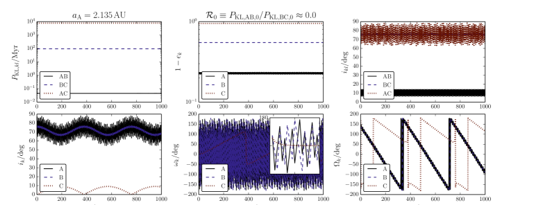
Refer to caption
Figure 13: Example evolution for the quadruple system ADS 1652 as discussed in Section 4.2.1, computed with SecularQuadruple. The parameters are given in Table 3; the currently unconstrained parameters pertaining to the outermost orbit, binary C, are eC=0.05subscript𝑒C0.05e_{\mathrm{C}}=0.05, iC=0subscript𝑖Csuperscript0i_{\mathrm{C}}=0^{\circ}, ωC=90.0subscript𝜔Csuperscript90.0\omega_{\mathrm{C}}=90.0^{\circ} and ΩC=130.0subscriptΩCsuperscript130.0\Omega_{\mathrm{C}}=130.0^{\circ}. In the bottom middle panel, the inset shows a magnification for t=0𝑡0t=0 to 20 Myr; note that both ωAsubscript𝜔A\omega_{\mathrm{A}} and ωBsubscript𝜔B\omega_{\mathrm{B}} are undersampled.

4.2 Application: observed stellar quadruples

4.2.1 ADS 1652

The quadruple system ADS 1652 (Tokovinin et al. 2014, and references therein) is composed of four main-sequence stars in the ‘3+1’ configuration. The system is likely old (age >GyrabsentGyr>\mathrm{Gyr}) considering the spectral types of its stellar components; the stars in binary A are of spectral type G9V, the star in binary B is of type K5V and the star in binary C is of type G8V. To date, ADS 1652 is one of few quadruple systems for which orbital fits have been obtained for multiple orbits.

m1subscript𝑚1m_{1} m2subscript𝑚2m_{2} m3subscript𝑚3m_{3} m4subscript𝑚4m_{4} aAsubscript𝑎Aa_{\mathrm{A}} aBsubscript𝑎Ba_{\mathrm{B}} aCsubscript𝑎Ca_{\mathrm{C}} eAsubscript𝑒Ae_{\mathrm{A}} eBsubscript𝑒Be_{\mathrm{B}} eCsubscript𝑒Ce_{\mathrm{C}} iAsubscript𝑖Ai_{\mathrm{A}} iBsubscript𝑖Bi_{\mathrm{B}} iCsubscript𝑖Ci_{\mathrm{C}} ωAsubscript𝜔A\omega_{\mathrm{A}} ωBsubscript𝜔B\omega_{\mathrm{B}} ωCsubscript𝜔C\omega_{\mathrm{C}} ΩAsubscriptΩA\Omega_{\mathrm{A}} ΩBsubscriptΩB\Omega_{\mathrm{B}} ΩCsubscriptΩC\Omega_{\mathrm{C}}
0.74 0.72 0.57 0.78 2.135 45.2 2500 0.769 0.45 75.9 76.0 287.9 175.0 127.2 140.0
Table 3: Parameters of the quadruple system ADS 1652 discussed in Section 4.2.1, adopted from Tokovinin et al. (2014), who fitted radial velocity and speckle measurements to the orbits of binaries A and B. The masses are obtained from these orbital fits (cf. the bottom row of table 7 of Tokovinin et al. 2014), the semimajor axes of the A and B binaries are computed from the fitted orbital periods (cf. table 4 of Tokovinin et al. 2014) using Kepler’s law. The eccentricity and orbital orientation of binary C are unknown (indicated with dashes), and are sampled with a Monte Carlo method in Section 4.2.1. Masses are expressed in solar masses, semimajor axes in AU, and angles in degrees.

Here, we apply the SecularQuadruple algorithm to ADS 1652 to explore its long-term secular dynamical evolution. We adopt the parameters that were obtained by Tokovinin et al. (2014), who fitted radial velocity and speckle measurements to the orbits of binaries A and B, and which are given in Table 3. Here, we adopted the component masses obtained from the orbital fits (cf. the bottom row of table 7 of Tokovinin et al. 2014), and computed the semimajor axes of the A and B binaries from the orbital periods (cf. table 4 of Tokovinin et al. 2014) using Kepler’s law. For the semimajor axis of the C binary, we adopt the observed projected distance of 2500 AU from binary A. Owing to its long orbital period of 105yrsimilar-toabsentsuperscript105yr\sim 10^{5}\,\mathrm{yr}, the eccentricities and orbital angles of binary C are not known. Here, we proceed by sampling these quantities for 500 realizations of the system, where eCsubscript𝑒Ce_{\mathrm{C}} is sampled from a thermal distribution, iCsubscript𝑖Ci_{\mathrm{C}} from a distribution uniform in cos(iC)subscript𝑖C\cos(i_{\mathrm{C}}), and ωCsubscript𝜔C\omega_{\mathrm{C}} and ΩCsubscriptΩC\Omega_{\mathrm{C}} from a uniform distribution. In our integrations, we included terms up and including octupole order (excluding the cross term), and the 1PN relativistic precession terms in the three binaries. The integration time is 20PKL,BC20subscript𝑃KLBC20\,P_{\mathrm{KL,BC}}, which is typically a few Gyr (depending on eCsubscript𝑒Ce_{\mathrm{C}}).

We show in Fig. 13 the evolution of an example system, where eC=0.05subscript𝑒C0.05e_{\mathrm{C}}=0.05, iC=0subscript𝑖Csuperscript0i_{\mathrm{C}}=0^{\circ}, ωC=90.0subscript𝜔Csuperscript90.0\omega_{\mathrm{C}}=90.0^{\circ} and ΩC=130.0subscriptΩCsuperscript130.0\Omega_{\mathrm{C}}=130.0^{\circ}. For this value of eCsubscript𝑒Ce_{\mathrm{C}}, 06.7×1041subscript06.7superscript104much-less-than1\mathcal{R}_{0}\approx 6.7\times 10^{-4}\ll 1, therefore the system is in the regime in which the torque of binary B on binary A dominates compared to the torque of binary C on binary B. Indeed, binaries A and B, which are initially nearly coplanar, remain nearly coplanar during the evolution (cf. the top-right panel in Fig. 13). Consequently, the KL eccentricity oscillations in binary A are of a very low amplitude, i.e. eA,max0.779subscript𝑒Amax0.779e_{\mathrm{A,max}}\approx 0.779, whereas eA,0=0.769subscript𝑒A00.769e_{\mathrm{A,0}}=0.769. Furthermore, KL eccentricity oscillations in binary B, which is initially inclined with respect to binary C with iBC,070subscript𝑖BC0superscript70i_{\mathrm{BC,0}}\approx 70^{\circ}, are completely quenched. This can be attributed to the rapid precession induced in B binary by binary A, on the time-scale of PKL,AB4×102MyrPKL,BC102Myrsubscript𝑃KLAB4superscript102Myrmuch-less-thansubscript𝑃KLBCsuperscript102MyrP_{\mathrm{KL,AB}}\approx 4\times 10^{-2}\,\mathrm{Myr}\ll P_{\mathrm{KL,BC}}\approx 10^{2}\,\mathrm{Myr} (cf. the bottom middle panel of Fig. 13).

In Fig. 14, eC,0=0.05subscript𝑒C00.05e_{\mathrm{C,0}}=0.05 was assumed to be low. The quantity 0subscript0\mathcal{R}_{0} increases with increasing eC,0subscript𝑒C0e_{\mathrm{C,0}} (cf. equation 3.3). Therefore, for larger eC,0subscript𝑒C0e_{\mathrm{C,0}}, the system could be in a very different regime in 0subscript0\mathcal{R}_{0} in which the evolution is very different. This is not the case in our Monte Carlo realizations, however, for which the mean and standard deviations of 0subscript0\mathcal{R}_{0} are 1.4×10³absent1.4superscript103\approx 1.4\times 10^{-3} and 1.0×10³absent1.0superscript103\approx 1.0\times 10^{-3}, respectively. In Fig. 14, we show for the 500 integrations the maximum eccentricities in the A and B binaries, and the minimum and maximum inclinations between binaries A and B. There is very small spread in all of these quantities, showing that their dependence on eCsubscript𝑒Ce_{\mathrm{C}}, as well as iCsubscript𝑖Ci_{\mathrm{C}}, ωCsubscript𝜔C\omega_{\mathrm{C}} and ΩCsubscriptΩC\Omega_{\mathrm{C}}, is very weak.

We conclude that, based on the observed state of ADS 1652, the eccentricities of its orbits will remain very nearly constant for, at least, the remainder of the main-sequence time-scale of its constituents. This conclusion is independent of the currently unknown eccentricity and orientation of the outermost orbit. In particular, even if the latter orbit is highly inclined with respect to the intermediate orbit, any potential KL eccentricity oscillations in the intermediate orbit are efficiently quenched.
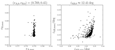
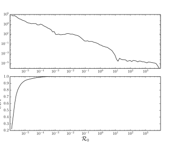
Refer to caption
Figure 14: The maximum eccentricities in the A and B binaries (left-hand panel), and the minimum and maximum inclinations between binaries A and B (right-hand panel), computed from numerical integrations with SecularQuadruple of 500 realizations of ADS 1652, where the parameters of the outermost orbit were varied (except aCsubscript𝑎Ca_{\mathrm{C}}). The dependence on the latter parameters is very weak.
Refer to caption
Figure 15: The distribution of the values of 0subscript0\mathcal{R}_{0} for the ‘3+1’ quadruple systems in the catalogue of Tokovinin (2014a, b), obtained by sampling, in 1000 realizations, eBsubscript𝑒Be_{\mathrm{B}} and eCsubscript𝑒Ce_{\mathrm{C}} from a thermal distribution. The probability (cumulative) density function is shown in the top (bottom) panel. For the majority of systems (0.9absent0.9\approx 0.9), 0<105subscript0superscript105\mathcal{R}_{0}<10^{-5} is small.

4.2.2 The Tokovinin sample of nearby FG dwarfs

As mentioned in Section 1, 55 of the 4847 observed systems of FG dwarfs in the catalogue of Tokovinin (2014a, b) are quadruple systems. From these, 18 are in the ‘3+1’ configuration, and for 13 of the latter, orbital periods and component masses are known for all three binaries. Here, we briefly explore in which dynamical regimes we expect these systems to be, by computing the associated value of 0subscript0\mathcal{R}_{0} (cf. Section 3.3).

For the 13 systems mentioned above, the orbital elements, apart from the semimajor axes, are unknown. In order to compute 0subscript0\mathcal{R}_{0}, the eccentricities eBsubscript𝑒Be_{\mathrm{B}} and eCsubscript𝑒Ce_{\mathrm{C}} are required (cf. equation 3.3). Therefore, for each of the 13 systems, we sample, in 1000 realizations, eBsubscript𝑒Be_{\mathrm{B}} and eCsubscript𝑒Ce_{\mathrm{C}} from a thermal distribution. Here, we reject sampled eccentricities if either of the AB and BC pair would be unstable according to the dynamical stability criterion of Mardling & Aarseth (2001).

The distribution of the values of 0subscript0\mathcal{R}_{0} obtained in this approach is shown in Fig. 15. The ratio 0subscript0\mathcal{R}_{0} is typically small; 0.9absent0.9\approx 0.9 of the sampled systems have 0<105subscript0superscript105\mathcal{R}_{0}<10^{-5}. This is the regime in which the AB pair is effectively an isolated triple, and where induced precession of binary A on binary B quenches KL eccentricity oscillations in binary B, as a consequence of the torque of binary C.

We note that one might expect currently observed quadruples not to be in the regime 01similar-tosubscript01\mathcal{R}_{0}\sim 1. If 01similar-tosubscript01\mathcal{R}_{0}\sim 1, then the large eccentricities in the innermost binary would likely already have strongly affected the system, and possibly have resulted in a merger. Evidently, in this case, the system would not have been observed as a quadruple system, but as a triple system. Conversely, some of the observed quadruple systems may have been quintuple systems in the past, and, triggered by secular dynamical evolution, evolved into quadruple systems through the merging of the stars in (likely) the shortest-period binary.

5 Conclusions

We have explored the global gravitational dynamics of hierarchical quadruple systems consisting of a hierarchical triple system orbited by a fourth body. Our main conclusions are as follows.

1. The Hamiltonian for the system has been derived and expanded to up and including fourth order in the ratios of the binary separations rA/rBsubscript𝑟Asubscript𝑟Br_{\mathrm{A}}/r_{\mathrm{B}}, rB/rCsubscript𝑟Bsubscript𝑟Cr_{\mathrm{B}}/r_{\mathrm{C}} and rA/rCsubscript𝑟Asubscript𝑟Cr_{\mathrm{A}}/r_{\mathrm{C}} (cf. Fig. 1). At each order, we have found three terms that are each mathematically equivalent to the corresponding terms that appear in the hierarchical three-body problem, and that depend on the properties of only two binaries. In addition to these terms, for octupole and higher orders, we have found ‘cross terms’ that depend on properties of all three binaries. Subsequently, we have derived expressions for the orbit-averaged Hamiltonian. A preliminary analysis indicates that the cross terms are typically not important in highly hierarchical systems on short time-scales, i.e. not exceeding time-scales of order PKL,BCsubscript𝑃KLBCP_{\mathrm{KL,BC}}, where PKL,BCsubscript𝑃KLBCP_{\mathrm{KL,BC}} is the KL time-scale of the BC pair. We have also derived the Hamiltonian for the configuration of two binaries orbiting each other’s barycentre (Appendix A.2).

2. For highly hierarchical systems, i.e. in which the three binaries are widely separated, the global dynamics can be qualitatively described in terms of the (initial) ratio of the KL time-scales of the AB to the BC pairs, 0PKL,AB,0/PKL,BC,0subscript0subscript𝑃KLAB0subscript𝑃KLBC0\mathcal{R}_{0}\equiv P_{\mathrm{KL,AB,0}}/P_{\mathrm{KL,BC,0}}.

If 01much-less-thansubscript01\mathcal{R}_{0}\ll 1, the torque of binary B on A dominates compared to the torque of binary C on binary B, and therefore binaries A and B remain coplanar if this was initially the case. If binaries A and B are initially inclined, KL eccentricity oscillations in binary A are not much affected by the presence of the fourth body. Eccentricity oscillations in binary B are efficiently quenched due to short time-scale precession induced on binary B by binary A.

If 01much-greater-thansubscript01\mathcal{R}_{0}\gg 1, the torque of binary C on binary B dominates compared to the torque of binary B on binary A. Initially, the inclination of binary B changes, whereas this is not the case for binary A. This induces a mutual inclination between binaries A and B, even if they are initially not inclined. However, rapid precession of binary B compared to the KL time-scale for the AB pair prevents any significant eccentricity oscillations in binary A, and even quenches KL oscillations if binaries A and B are initially inclined.

Lastly, if 01similar-tosubscript01\mathcal{R}_{0}\sim 1, complex KL eccentricity oscillations occur in binary A that are strongly coupled with the KL eccentricity oscillations in binary B. The latter are also affected compared to the situation in which binary A were replaced by a point mass, although this is typically a much smaller effect. Even if binaries A and B are initially coplanar, the induced inclination can result in very high eccentricity oscillations in binary A. These extreme eccentricities could have significant implications for strong interactions such as tidal interactions, gravitational wave dissipation, and collisions and mergers of stars and compact objects.

3. We also included the effects of general relativity, in particular relativistic precession. We have found that the range in the parameter space of the semimajor axis ratios aB/aAsubscript𝑎Bsubscript𝑎Aa_{\mathrm{B}}/a_{\mathrm{A}} for which KL oscillations are important in binary A can be extended compared to hierarchical triple systems. This is due to a decrease of the KL time-scale of the AB pair when the eccentricity of binary B is at a maximum.

4. We have applied our results to a planetary configuration consisting of a planet+moon system orbiting a central star that is orbited by a more distant and inclined binary companion. We have found that there are regions in parameter space where a planet+moon system that is initially coplanar with respect to the central star, can become inclined and the eccentricity in the planet+moon system can be excited. This could result in significant tidal dissipation and even a collision of the planet with its moon. Furthermore, when the orbit of the binary companion is wide, KL eccentricity oscillations in the orbit of the planet+moon system around the central star can be quenched because of induced precession from the planet+moon system. This effectively shields the planet from high-eccentricity KL oscillations from a binary companion, and, therefore, potential disruption by the central star could be avoided.

5. Lastly, we applied our results to stellar quadruple systems. In the case of ADS 1652, 0103similar-tosubscript0superscript103\mathcal{R}_{0}\sim 10^{-3} assuming a thermal distribution of the unknown eCsubscript𝑒Ce_{\mathrm{C}}, and we find almost negligible KL eccentricity oscillations in both the innermost and intermediate orbits, binaries A and B. Even if the outer orbit, binary C, were highly inclined with respect to binary B, any potential KL eccentricity oscillations in binary B would be efficiently quenched.

For the ‘3+1’ FG stellar quadruples in the catalogue of Tokovinin (2014a, b), we estimate 0.9absent0.9\approx 0.9 of the systems to have 0<105subscript0superscript105\mathcal{R}_{0}<10^{-5}. Therefore, we expect that in the majority of these systems, KL eccentricity oscillations in the BC pair are quenched, and, from a secular dynamical point of view, the innermost AB pair can be considered as an isolated triple.

Acknowledgements

We thank the referee, Smadar Naoz, for providing very helpful comments that lead to improvement of the paper. This work was initiated during the International Summer-Institute for Modeling in Astrophysics (ISIMA) in 2014, hosted at CITA at the University of Toronto. It was supported by the Netherlands Research Council NWO (grants #639.073.803 [VICI], #614.061.608 [AMUSE] and #612.071.305 [LGM]) and the Netherlands Research School for Astronomy (NOVA). HBP acknowledges support from the ISF I-CORE programme 1829, The European FP-7 CIG programme ‘GRAND’ (333644), the BSF grant number 2012384 and the Asher foundation.

References

  • Allan & Cook (1964) Allan R. R., Cook G. E., 1964, Royal Society of London Proceedings Series A, 280, 97
  • Allan & Ward (1963) Allan R. R., Ward G. N., 1963, Proceedings of the Cambridge Philosophical Society, 59, 669
  • Antognini et al. (2014) Antognini J. M., Shappee B. J., Thompson T. A., Amaro-Seoane P., 2014, MNRAS, 439, 1079
  • Antonini & Perets (2012) Antonini F., Perets H. B., 2012, ApJ, 757, 27
  • Antonini et al. (2014) Antonini F., Murray N., Mikkola S., 2014, ApJ, 781, 45
  • Blaes et al. (2002) Blaes O., Lee M. H., Socrates A., 2002, ApJ, 578, 775
  • Boué & Fabrycky (2014) Boué G., Fabrycky D. C., 2014, ApJ, 789, 110
  • Breiter & Ratajczak (2005) Breiter S., Ratajczak R., 2005, MNRAS, 364, 1222
  • Brouwer (1959) Brouwer D., 1959, AJ, 64, 378
  • Chirikov (1979) Chirikov B. V., 1979, Phys. Rep., 52, 263
  • Cohen et al. (1996) Cohen S. D., Hindmarsh A. C., Dubois P. F., 1996, Computers in Physics, 10, 138
  • Correia et al. (2011) Correia A. C. M., Laskar J., Farago F., Boué G., 2011, Celestial Mechanics and Dynamical Astronomy, 111, 105
  • Eggleton & Kiseleva-Eggleton (2001) Eggleton P. P., Kiseleva-Eggleton L., 2001, ApJ, 562, 1012
  • Eggleton & Kisseleva-Eggleton (2006) Eggleton P. P., Kisseleva-Eggleton L., 2006, Ap&SS, 304, 75
  • Fabrycky & Tremaine (2007) Fabrycky D., Tremaine S., 2007, ApJ, 669, 1298
  • Ford et al. (2000) Ford E. B., Kozinsky B., Rasio F. A., 2000, ApJ, 535, 385
  • Goldstein (1975) Goldstein H., 1975, American Journal of Physics, 43, 737
  • Goldstein (1976) Goldstein H., 1976, American Journal of Physics, 44, 1123
  • Goldstein et al. (2002) Goldstein H., Poole C., Safko J., 2002, Classical mechanics
  • Gonçalves Ferrari et al. (2014) Gonçalves Ferrari G., Boekholt T., Portegies Zwart S. F., 2014, MNRAS, 440, 719
  • Hamers et al. (2013) Hamers A. S., Pols O. R., Claeys J. S. W., Nelemans G., 2013, MNRAS, 430, 2262
  • Harrington (1968) Harrington R. S., 1968, AJ, 73, 190
  • Harrington (1969) Harrington R. S., 1969, Celestial Mechanics, 1, 200
  • Innanen et al. (1997) Innanen K. A., Zheng J. Q., Mikkola S., Valtonen M. J., 1997, AJ, 113, 1915
  • Katz & Dong (2012) Katz B., Dong S., 2012, preprint, (arXiv:1211.4584)
  • Katz et al. (2011) Katz B., Dong S., Malhotra R., 2011, Physical Review Letters, 107, 181101
  • Kolmogorov (1933) Kolmogorov A., 1933, G. Ist. Ital. Attuari, 4, 83
  • Kozai (1962) Kozai Y., 1962, AJ, 67, 591
  • Laskar & Boué (2010) Laskar J., Boué G., 2010, A&A, 522, A60
  • Li et al. (2014a) Li G., Naoz S., Kocsis B., Loeb A., 2014a, ApJ, 785, 116
  • Li et al. (2014b) Li G., Naoz S., Holman M., Loeb A., 2014b, ApJ, 791, 86
  • Lidov (1962) Lidov M. L., 1962, Planet. Space Sci., 9, 719
  • Lithwick & Naoz (2011) Lithwick Y., Naoz S., 2011, ApJ, 742, 94
  • Mardling & Aarseth (2001) Mardling R. A., Aarseth S. J., 2001, MNRAS, 321, 398
  • Mikkola & Merritt (2008) Mikkola S., Merritt D., 2008, AJ, 135, 2398
  • Milankovitch (1939) Milankovitch M., 1939, Bull. Serb. Acad. Math. Nat., 6
  • Miller & Hamilton (2002) Miller M. C., Hamilton D. P., 2002, ApJ, 576, 894
  • Musen (1961) Musen P., 1961, J. Geophys. Res., 66, 2797
  • Naoz & Fabrycky (2014) Naoz S., Fabrycky D. C., 2014, ApJ, 793, 137
  • Naoz et al. (2011) Naoz S., Farr W. M., Lithwick Y., Rasio F. A., Teyssandier J., 2011, Nature, 473, 187
  • Naoz et al. (2012) Naoz S., Farr W. M., Rasio F. A., 2012, ApJ, 754, L36
  • Naoz et al. (2013a) Naoz S., Farr W. M., Lithwick Y., Rasio F. A., Teyssandier J., 2013a, MNRAS, 431, 2155
  • Naoz et al. (2013b) Naoz S., Kocsis B., Loeb A., Yunes N., 2013b, ApJ, 773, 187
  • Pejcha et al. (2013) Pejcha O., Antognini J. M., Shappee B. J., Thompson T. A., 2013, MNRAS, 435, 943
  • Pelupessy et al. (2013) Pelupessy F. I., van Elteren A., de Vries N., McMillan S. L. W., Drost N., Portegies Zwart S. F., 2013, A&A, 557, A84
  • Perets & Fabrycky (2009) Perets H. B., Fabrycky D. C., 2009, ApJ, 697, 1048
  • Perets & Naoz (2009) Perets H. B., Naoz S., 2009, ApJ, 699, L17
  • Petrovich (2014) Petrovich C., 2014, preprint, (arXiv:1405.0280)
  • Portegies Zwart et al. (2013) Portegies Zwart S., McMillan S. L. W., van Elteren E., Pelupessy I., de Vries N., 2013, Computer Physics Communications, 183, 456
  • Prodan et al. (2013) Prodan S., Murray N., Thompson T. A., 2013, preprint, (arXiv:1305.2191)
  • Rosengren & Scheeres (2014) Rosengren A. J., Scheeres D. J., 2014, Celestial Mechanics and Dynamical Astronomy, 118, 197
  • Schwarzschild (1916) Schwarzschild K., 1916, Abh. Konigl. Preuss. Akad. Wissenschaften Jahre 1906,92, Berlin,1907, 1916, 189
  • Smirnov (1948) Smirnov N., 1948, Annals of Mathematical Statistics, 19, 279
  • Takeda & Rasio (2005) Takeda G., Rasio F. A., 2005, ApJ, 627, 1001
  • Takeda et al. (2008) Takeda G., Kita R., Rasio F. A., 2008, ApJ, 683, 1063
  • Teyssandier et al. (2013) Teyssandier J., Naoz S., Lizarraga I., Rasio F. A., 2013, ApJ, 779, 166
  • Thompson (2011) Thompson T. A., 2011, ApJ, 741, 82
  • Tokovinin (2014a) Tokovinin A., 2014a, AJ, 147, 86
  • Tokovinin (2014b) Tokovinin A., 2014b, AJ, 147, 87
  • Tokovinin et al. (2014) Tokovinin A., Gorynya N. A., Morrell N. I., 2014, MNRAS, 443, 3082
  • Touma et al. (2009) Touma J. R., Tremaine S., Kazandjian M. V., 2009, MNRAS, 394, 1085
  • Tremaine et al. (2009) Tremaine S., Touma J., Namouni F., 2009, AJ, 137, 3706
  • Will (2014a) Will C. M., 2014a, preprint, (arXiv:1404.7724)
  • Will (2014b) Will C. M., 2014b, Phys. Rev. D, 89, 044043
  • Wu & Murray (2003) Wu Y., Murray N., 2003, ApJ, 589, 605
  • Wu et al. (2007) Wu Y., Murray N. W., Ramsahai J. M., 2007, ApJ, 670, 820

Appendix A The Hamiltonian for hierarchical quadruple systems

The general Newtonian four-body Hamiltonian is given by

H=T+U=12i=14mi𝑽i212i,j;ijGmimj𝑹i𝑹j,𝐻𝑇𝑈12superscriptsubscript𝑖14subscript𝑚𝑖superscriptsubscript𝑽𝑖212subscript𝑖𝑗𝑖𝑗𝐺subscript𝑚𝑖subscript𝑚𝑗normsubscript𝑹𝑖subscript𝑹𝑗\displaystyle H=T+U=\frac{1}{2}\sum_{i=1}^{4}m_{i}\boldsymbol{V}_{i}^{2}-\frac{1}{2}\sum_{i,j;i\neq j}\frac{Gm_{i}m_{j}}{||\boldsymbol{R}_{i}-\boldsymbol{R}_{j}||}, (24)

where misubscript𝑚𝑖m_{i}, 𝑹isubscript𝑹𝑖\boldsymbol{R}_{i} and 𝑽isubscript𝑽𝑖\boldsymbol{V}_{i} denote the mass and position and velocity vectors of body i𝑖i. Here, we consider dynamically stable hierarchical configurations. For four bodies, these consist of (1) a hierarchical triple system orbited by a fourth body in an orbit around the triple (discussed in detail in the main text), and (2) two binary systems orbiting each other’s centre of mass. Below we discuss both configurations separately.

A.1 Hierarchical triple system orbited by a fourth body

In this configuration, we assume that bodies 1 and 2 are bound in binary A, body 3 is bound to the barycentre of bodies 1 and 2 in binary B, and body 4 is bound to the barycentre of bodies 1, 2 and 3 in binary C. It is convenient to define the following separation vectors,

𝒓Asubscript𝒓A\displaystyle\boldsymbol{r}_{\mathrm{A}} 𝑹1𝑹2;absentsubscript𝑹1subscript𝑹2\displaystyle\equiv\boldsymbol{R}_{1}-\boldsymbol{R}_{2}; (25a)
𝒓Bsubscript𝒓B\displaystyle\boldsymbol{r}_{\mathrm{B}} m1𝑹1+m2𝑹2m1+m2𝑹3;absentsubscript𝑚1subscript𝑹1subscript𝑚2subscript𝑹2subscript𝑚1subscript𝑚2subscript𝑹3\displaystyle\equiv\frac{m_{1}\boldsymbol{R}_{1}+m_{2}\boldsymbol{R}_{2}}{m_{1}+m_{2}}-\boldsymbol{R}_{3}; (25b)
𝒓Csubscript𝒓C\displaystyle\boldsymbol{r}_{\mathrm{C}} m1𝑹1+m2𝑹2+m3𝑹3m1+m2+m3𝑹4.absentsubscript𝑚1subscript𝑹1subscript𝑚2subscript𝑹2subscript𝑚3subscript𝑹3subscript𝑚1subscript𝑚2subscript𝑚3subscript𝑹4\displaystyle\equiv\frac{m_{1}\boldsymbol{R}_{1}+m_{2}\boldsymbol{R}_{2}+m_{3}\boldsymbol{R}_{3}}{m_{1}+m_{2}+m_{3}}-\boldsymbol{R}_{4}. (25c)

In addition, we define the centre of mass position of the four-body system,

𝒓CM[i=14mi]1i=14mi𝑹i,subscript𝒓CMsuperscriptdelimited-[]superscriptsubscript𝑖14subscript𝑚𝑖1superscriptsubscript𝑖14subscript𝑚𝑖subscript𝑹𝑖\displaystyle\boldsymbol{r}_{\mathrm{CM}}\equiv\left[\sum_{i=1}^{4}m_{i}\right]^{-1}\sum_{i=1}^{4}m_{i}\boldsymbol{R}_{i}, (26)

which satisfies 𝒓˙CM=𝟎subscript˙𝒓CM0\dot{\boldsymbol{r}}_{\mathrm{CM}}=\boldsymbol{0}. Equations (25) and (26) are easily inverted to give 𝑹isubscript𝑹𝑖\boldsymbol{R}_{i} in terms of 𝒓Asubscript𝒓A\boldsymbol{r}_{\mathrm{A}}, 𝒓Bsubscript𝒓B\boldsymbol{r}_{\mathrm{B}}, 𝒓Csubscript𝒓C\boldsymbol{r}_{\mathrm{C}} and 𝒓CMsubscript𝒓CM\boldsymbol{r}_{\mathrm{CM}}. Differentiating the resulting relations with respect to time, and assuming that the masses are constant, we find for the kinetic energy

T=12m1m2m1+m2𝒓˙A2+12(m1+m2)m3m1+m2+m3𝒓˙B2+12(m1+m2+m3)m4m1+m2+m3+m4𝒓˙C2.𝑇12subscript𝑚1subscript𝑚2subscript𝑚1subscript𝑚2superscriptsubscript˙𝒓A212subscript𝑚1subscript𝑚2subscript𝑚3subscript𝑚1subscript𝑚2subscript𝑚3superscriptsubscript˙𝒓B212subscript𝑚1subscript𝑚2subscript𝑚3subscript𝑚4subscript𝑚1subscript𝑚2subscript𝑚3subscript𝑚4superscriptsubscript˙𝒓C2\displaystyle T=\frac{1}{2}\frac{m_{1}m_{2}}{m_{1}+m_{2}}\dot{\boldsymbol{r}}_{\mathrm{A}}^{2}+\frac{1}{2}\frac{(m_{1}+m_{2})m_{3}}{m_{1}+m_{2}+m_{3}}\dot{\boldsymbol{r}}_{\mathrm{B}}^{2}+\frac{1}{2}\frac{(m_{1}+m_{2}+m_{3})m_{4}}{m_{1}+m_{2}+m_{3}+m_{4}}\dot{\boldsymbol{r}}_{\mathrm{C}}^{2}. (27)

To find the potential, we similarly invert equations (25) to give the difference vectors 𝑹i𝑹jnormsubscript𝑹𝑖subscript𝑹𝑗||\boldsymbol{R}_{i}-\boldsymbol{R}_{j}|| in terms of 𝒓Asubscript𝒓A\boldsymbol{r}_{\mathrm{A}}, 𝒓Bsubscript𝒓B\boldsymbol{r}_{\mathrm{B}} and 𝒓Csubscript𝒓C\boldsymbol{r}_{\mathrm{C}}. Substituting the resulting relations into the potential U𝑈U yields six terms each of the form

𝒓C+α𝒓B+β𝒓A1,𝒓C+α𝒓B1and𝒓B+β𝒓A1,superscriptnormsubscript𝒓C𝛼subscript𝒓B𝛽subscript𝒓A1superscriptnormsubscript𝒓C𝛼subscript𝒓B1andsuperscriptnormsubscript𝒓B𝛽subscript𝒓A1\displaystyle{||\boldsymbol{r}_{\mathrm{C}}+\alpha\boldsymbol{r}_{\mathrm{B}}+\beta\boldsymbol{r}_{\mathrm{A}}||}^{-1},\quad{||\boldsymbol{r}_{\mathrm{C}}+\alpha\boldsymbol{r}_{\mathrm{B}}||}^{-1}\quad\mathrm{and}\quad{||\boldsymbol{r}_{\mathrm{B}}+\beta\boldsymbol{r}_{\mathrm{A}}||}^{-1},

where α𝛼\alpha and β𝛽\beta, which can be negative, are various mass ratios. We will assume that rC|α|rB|β|rAmuch-greater-thansubscript𝑟C𝛼subscript𝑟Bmuch-greater-than𝛽subscript𝑟Ar_{\mathrm{C}}\gg|\alpha|r_{\mathrm{B}}\gg|\beta|r_{\mathrm{A}} (where r𝒓𝑟norm𝒓r\equiv||\boldsymbol{r}||). In other words, we will assume that the system is sufficiently hierarchical in the sense that it is appropriate to expand the potential in terms of the relative distance ratios rA/rBsubscript𝑟Asubscript𝑟Br_{\mathrm{A}}/r_{\mathrm{B}}, rB/rCsubscript𝑟Bsubscript𝑟Cr_{\mathrm{B}}/r_{\mathrm{C}} and rA/rCsubscript𝑟Asubscript𝑟Cr_{\mathrm{A}}/r_{\mathrm{C}}, all of which are assumed to be small, and that the mass ratios are not too extreme.

We expand the potential in terms of the relative distance ratios using the general expansion

||𝒓+α𝒓+β𝒓′′||1=1r[1α(rr)(𝒓^𝒓^)β(r′′r)(𝒓^𝒓^′′)+12α2(rr)2{3(𝒓^𝒓^)21}+12β2(r′′r)2{3(𝒓^𝒓^′′)21}\displaystyle{||\boldsymbol{r}+\alpha\boldsymbol{r}^{\prime}+\beta\boldsymbol{r}^{\prime\prime}||}^{-1}=\frac{1}{r}\left[1-\alpha\left(\frac{r^{\prime}}{r}\right)\left(\hat{\boldsymbol{r}}\cdot\hat{\boldsymbol{r}}^{\prime}\right)-\beta\left(\frac{r^{\prime\prime}}{r}\right)\left(\hat{\boldsymbol{r}}\cdot\hat{\boldsymbol{r}}^{\prime\prime}\right)+\frac{1}{2}\alpha^{2}\left(\frac{r^{\prime}}{r}\right)^{2}\left\{3\left(\hat{\boldsymbol{r}}\cdot\hat{\boldsymbol{r}}^{\prime}\right)^{2}-1\right\}+\frac{1}{2}\beta^{2}\left(\frac{r^{\prime\prime}}{r}\right)^{2}\left\{3\left(\hat{\boldsymbol{r}}\cdot\hat{\boldsymbol{r}}^{\prime\prime}\right)^{2}-1\right\}\right.
+αβ(rr)(r′′r){3(𝒓^𝒓^)(𝒓^𝒓^′′)(𝒓^𝒓^)}12α3(rr)3{5(𝒓^𝒓^)33(𝒓^𝒓^)}12β3(r′′r)3{5(𝒓^𝒓^′′)33(𝒓^𝒓^′′)}𝛼𝛽superscript𝑟𝑟superscript𝑟′′𝑟3^𝒓superscript^𝒓^𝒓superscript^𝒓′′superscript^𝒓superscript^𝒓12superscript𝛼3superscriptsuperscript𝑟𝑟35superscript^𝒓superscript^𝒓33^𝒓superscript^𝒓12superscript𝛽3superscriptsuperscript𝑟′′𝑟35superscript^𝒓superscript^𝒓′′33^𝒓superscript^𝒓′′\displaystyle\quad\left.+\alpha\beta\left(\frac{r^{\prime}}{r}\right)\left(\frac{r^{\prime\prime}}{r}\right)\left\{3\left(\hat{\boldsymbol{r}}\cdot\hat{\boldsymbol{r}}^{\prime}\right)\left(\hat{\boldsymbol{r}}\cdot\hat{\boldsymbol{r}}^{\prime\prime}\right)-\left(\hat{\boldsymbol{r}}^{\prime}\cdot\hat{\boldsymbol{r}}^{\prime}\right)\right\}-\frac{1}{2}\alpha^{3}\left(\frac{r^{\prime}}{r}\right)^{3}\left\{5\left(\hat{\boldsymbol{r}}\cdot\hat{\boldsymbol{r}}^{\prime}\right)^{3}-3\left(\hat{\boldsymbol{r}}\cdot\hat{\boldsymbol{r}}^{\prime}\right)\right\}-\frac{1}{2}\beta^{3}\left(\frac{r^{\prime\prime}}{r}\right)^{3}\left\{5\left(\hat{\boldsymbol{r}}\cdot\hat{\boldsymbol{r}}^{\prime\prime}\right)^{3}-3\left(\hat{\boldsymbol{r}}\cdot\hat{\boldsymbol{r}}^{\prime\prime}\right)\right\}\right.
12α2β(rr)2(r′′r){15(𝒓^𝒓^)2(𝒓^𝒓^′′)3(𝒓^𝒓^′′)6(𝒓^𝒓^)(𝒓^𝒓^′′)}12superscript𝛼2𝛽superscriptsuperscript𝑟𝑟2superscript𝑟′′𝑟15superscript^𝒓superscript^𝒓2^𝒓superscript^𝒓′′3^𝒓superscript^𝒓′′6^𝒓superscript^𝒓superscript^𝒓superscript^𝒓′′\displaystyle\quad\left.-\frac{1}{2}\alpha^{2}\beta\left(\frac{r^{\prime}}{r}\right)^{2}\left(\frac{r^{\prime\prime}}{r}\right)\left\{15\left(\hat{\boldsymbol{r}}\cdot\hat{\boldsymbol{r}}^{\prime}\right)^{2}\left(\hat{\boldsymbol{r}}\cdot\hat{\boldsymbol{r}}^{\prime\prime}\right)-3\left(\hat{\boldsymbol{r}}\cdot\hat{\boldsymbol{r}}^{\prime\prime}\right)-6\left(\hat{\boldsymbol{r}}\cdot\hat{\boldsymbol{r}}^{\prime}\right)\left(\hat{\boldsymbol{r}}^{\prime}\cdot\hat{\boldsymbol{r}}^{\prime\prime}\right)\right\}\right.
12αβ2(rr)(r′′r)2{15(𝒓^𝒓^′′)2(𝒓^𝒓^)3(𝒓^𝒓^)6(𝒓^𝒓^′′)(𝒓^𝒓^′′)}12𝛼superscript𝛽2superscript𝑟𝑟superscriptsuperscript𝑟′′𝑟215superscript^𝒓superscript^𝒓′′2^𝒓superscript^𝒓3^𝒓superscript^𝒓6^𝒓superscript^𝒓′′superscript^𝒓superscript^𝒓′′\displaystyle\quad\left.-\frac{1}{2}\alpha\beta^{2}\left(\frac{r^{\prime}}{r}\right)\left(\frac{r^{\prime\prime}}{r}\right)^{2}\left\{15\left(\hat{\boldsymbol{r}}\cdot\hat{\boldsymbol{r}}^{\prime\prime}\right)^{2}\left(\hat{\boldsymbol{r}}\cdot\hat{\boldsymbol{r}}^{\prime}\right)-3\left(\hat{\boldsymbol{r}}\cdot\hat{\boldsymbol{r}}^{\prime}\right)-6\left(\hat{\boldsymbol{r}}\cdot\hat{\boldsymbol{r}}^{\prime\prime}\right)\left(\hat{\boldsymbol{r}}^{\prime}\cdot\hat{\boldsymbol{r}}^{\prime\prime}\right)\right\}\right.
+18α4(rr)4{330(𝒓^𝒓^)2+35(𝒓^𝒓^)4}+18β4(r′′r)4{330(𝒓^𝒓^′′)2+35(𝒓^𝒓^′′)4}]\displaystyle\quad\left.+\frac{1}{8}\alpha^{4}\left(\frac{r^{\prime}}{r}\right)^{4}\left\{3-30\left(\hat{\boldsymbol{r}}\cdot\hat{\boldsymbol{r}}^{\prime}\right)^{2}+35\left(\hat{\boldsymbol{r}}\cdot\hat{\boldsymbol{r}}^{\prime}\right)^{4}\right\}+\frac{1}{8}\beta^{4}\left(\frac{r^{\prime\prime}}{r}\right)^{4}\left\{3-30\left(\hat{\boldsymbol{r}}\cdot\hat{\boldsymbol{r}}^{\prime\prime}\right)^{2}+35\left(\hat{\boldsymbol{r}}\cdot\hat{\boldsymbol{r}}^{\prime\prime}\right)^{4}\right\}\right]
+12α3β(rr)3(r′′r){35(𝒓^𝒓^)3(𝒓^𝒓^′′)15(𝒓^𝒓^)2(𝒓^𝒓^′′)15(𝒓^𝒓^)(𝒓^𝒓^′′)+3(𝒓^𝒓^′′)}12superscript𝛼3𝛽superscriptsuperscript𝑟𝑟3superscript𝑟′′𝑟35superscript^𝒓superscript^𝒓3^𝒓superscript^𝒓′′15superscript^𝒓superscript^𝒓2superscript^𝒓superscript^𝒓′′15^𝒓superscript^𝒓^𝒓superscript^𝒓′′3superscript^𝒓superscript^𝒓′′\displaystyle\quad\left.+\frac{1}{2}\alpha^{3}\beta\left(\frac{r^{\prime}}{r}\right)^{3}\left(\frac{r^{\prime\prime}}{r}\right)\left\{35\left(\hat{\boldsymbol{r}}\cdot\hat{\boldsymbol{r}}^{\prime}\right)^{3}\left(\hat{\boldsymbol{r}}\cdot\hat{\boldsymbol{r}}^{\prime\prime}\right)-15\left(\hat{\boldsymbol{r}}\cdot\hat{\boldsymbol{r}}^{\prime}\right)^{2}\left(\hat{\boldsymbol{r}}^{\prime}\cdot\hat{\boldsymbol{r}}^{\prime\prime}\right)-15\left(\hat{\boldsymbol{r}}\cdot\hat{\boldsymbol{r}}^{\prime}\right)\left(\hat{\boldsymbol{r}}\cdot\hat{\boldsymbol{r}}^{\prime\prime}\right)+3\left(\hat{\boldsymbol{r}}^{\prime}\cdot\hat{\boldsymbol{r}}^{\prime\prime}\right)\right\}\right.
+12αβ3(rr)(r′′r)3{35(𝒓^𝒓^′′)3(𝒓^𝒓^)15(𝒓^𝒓^′′)2(𝒓^𝒓^′′)15(𝒓^𝒓^)(𝒓^𝒓^′′)+3(𝒓^𝒓^′′)}12𝛼superscript𝛽3superscript𝑟𝑟superscriptsuperscript𝑟′′𝑟335superscript^𝒓superscript^𝒓′′3^𝒓superscript^𝒓15superscript^𝒓superscript^𝒓′′2superscript^𝒓superscript^𝒓′′15^𝒓superscript^𝒓^𝒓superscript^𝒓′′3superscript^𝒓superscript^𝒓′′\displaystyle\quad\left.+\frac{1}{2}\alpha\beta^{3}\left(\frac{r^{\prime}}{r}\right)\left(\frac{r^{\prime\prime}}{r}\right)^{3}\left\{35\left(\hat{\boldsymbol{r}}\cdot\hat{\boldsymbol{r}}^{\prime\prime}\right)^{3}\left(\hat{\boldsymbol{r}}\cdot\hat{\boldsymbol{r}}^{\prime}\right)-15\left(\hat{\boldsymbol{r}}\cdot\hat{\boldsymbol{r}}^{\prime\prime}\right)^{2}\left(\hat{\boldsymbol{r}}^{\prime}\cdot\hat{\boldsymbol{r}}^{\prime\prime}\right)-15\left(\hat{\boldsymbol{r}}\cdot\hat{\boldsymbol{r}}^{\prime}\right)\left(\hat{\boldsymbol{r}}\cdot\hat{\boldsymbol{r}}^{\prime\prime}\right)+3\left(\hat{\boldsymbol{r}}^{\prime}\cdot\hat{\boldsymbol{r}}^{\prime\prime}\right)\right\}\right.
+14α2β2(rr)2(r′′r)2{105(𝒓^𝒓^)2(𝒓^𝒓^′′)215(𝒓^𝒓^)215(𝒓^𝒓^′′)215(𝒓^𝒓^)(𝒓^𝒓^′′)(𝒓^𝒓^′′)+3(𝒓^𝒓^′′)2+3}14superscript𝛼2superscript𝛽2superscriptsuperscript𝑟𝑟2superscriptsuperscript𝑟′′𝑟2105superscript^𝒓superscript^𝒓2superscript^𝒓superscript^𝒓′′215superscript^𝒓superscript^𝒓215superscript^𝒓superscript^𝒓′′215^𝒓superscript^𝒓^𝒓superscript^𝒓′′superscript^𝒓superscript^𝒓′′3superscriptsuperscript^𝒓superscript^𝒓′′23\displaystyle\quad\left.+\frac{1}{4}\alpha^{2}\beta^{2}\left(\frac{r^{\prime}}{r}\right)^{2}\left(\frac{r^{\prime\prime}}{r}\right)^{2}\left\{105\left(\hat{\boldsymbol{r}}\cdot\hat{\boldsymbol{r}}^{\prime}\right)^{2}\left(\hat{\boldsymbol{r}}\cdot\hat{\boldsymbol{r}}^{\prime\prime}\right)^{2}-15\left(\hat{\boldsymbol{r}}\cdot\hat{\boldsymbol{r}}^{\prime}\right)^{2}-15\left(\hat{\boldsymbol{r}}\cdot\hat{\boldsymbol{r}}^{\prime\prime}\right)^{2}-15\left(\hat{\boldsymbol{r}}\cdot\hat{\boldsymbol{r}}^{\prime}\right)\left(\hat{\boldsymbol{r}}\cdot\hat{\boldsymbol{r}}^{\prime\prime}\right)\left(\hat{\boldsymbol{r}}^{\prime}\cdot\hat{\boldsymbol{r}}^{\prime\prime}\right)+3\left(\hat{\boldsymbol{r}}^{\prime}\cdot\hat{\boldsymbol{r}}^{\prime\prime}\right)^{2}+3\right\}\right.
+𝒪{(rr)i(r′′r)j}].\displaystyle\quad\left.+\mathcal{O}\left\{\left(\frac{r^{\prime}}{r}\right)^{i}\left(\frac{r^{\prime\prime}}{r}\right)^{j}\right\}\right]. (28)

Here, i+j5𝑖𝑗5i+j\geq 5. Substituting this expansion into equation (24), we find

Htssubscript𝐻ts\displaystyle H_{\mathrm{ts}} =Hbin(m1,m2,𝒓A,𝒓˙A)+Hbin(m1+m2,m3,𝒓B,𝒓˙B)+Hbin(m1+m2+m3,m4,𝒓C,𝒓˙C)absentsubscript𝐻binsubscript𝑚1subscript𝑚2subscript𝒓Asubscript˙𝒓Asubscript𝐻binsubscript𝑚1subscript𝑚2subscript𝑚3subscript𝒓Bsubscript˙𝒓Bsubscript𝐻binsubscript𝑚1subscript𝑚2subscript𝑚3subscript𝑚4subscript𝒓Csubscript˙𝒓C\displaystyle=H_{\mathrm{bin}}(m_{1},m_{2},\boldsymbol{r}_{\mathrm{A}},\dot{\boldsymbol{r}}_{\mathrm{A}})+H_{\mathrm{bin}}(m_{1}+m_{2},m_{3},\boldsymbol{r}_{\mathrm{B}},\dot{\boldsymbol{r}}_{\mathrm{B}})+H_{\mathrm{bin}}(m_{1}+m_{2}+m_{3},m_{4},\boldsymbol{r}_{\mathrm{C}},\dot{\boldsymbol{r}}_{\mathrm{C}})
+Hquad(m1,m2,m3,𝒓A,𝒓B)+Hquad(m1+m2,m3,m4,𝒓B,𝒓C)+Hquad(m1,m2,m4,𝒓A,𝒓C)subscript𝐻quadsubscript𝑚1subscript𝑚2subscript𝑚3subscript𝒓Asubscript𝒓Bsubscript𝐻quadsubscript𝑚1subscript𝑚2subscript𝑚3subscript𝑚4subscript𝒓Bsubscript𝒓Csubscript𝐻quadsubscript𝑚1subscript𝑚2subscript𝑚4subscript𝒓Asubscript𝒓C\displaystyle\quad+H_{\mathrm{quad}}(m_{1},m_{2},m_{3},\boldsymbol{r}_{\mathrm{A}},\boldsymbol{r}_{\mathrm{B}})+H_{\mathrm{quad}}(m_{1}+m_{2},m_{3},m_{4},\boldsymbol{r}_{\mathrm{B}},\boldsymbol{r}_{\mathrm{C}})+H_{\mathrm{quad}}(m_{1},m_{2},m_{4},\boldsymbol{r}_{\mathrm{A}},\boldsymbol{r}_{\mathrm{C}})
+Hoct(m1,m2,m3,𝒓A,𝒓B)+Hoct(m1+m2,m3,m4,𝒓B,𝒓C)+Hoct(m1,m2,m4,𝒓A,𝒓C)subscript𝐻octsubscript𝑚1subscript𝑚2subscript𝑚3subscript𝒓Asubscript𝒓Bsubscript𝐻octsubscript𝑚1subscript𝑚2subscript𝑚3subscript𝑚4subscript𝒓Bsubscript𝒓Csubscript𝐻octsubscript𝑚1subscript𝑚2subscript𝑚4subscript𝒓Asubscript𝒓C\displaystyle\quad+H_{\mathrm{oct}}(m_{1},m_{2},m_{3},\boldsymbol{r}_{\mathrm{A}},\boldsymbol{r}_{\mathrm{B}})+H_{\mathrm{oct}}(m_{1}+m_{2},m_{3},m_{4},\boldsymbol{r}_{\mathrm{B}},\boldsymbol{r}_{\mathrm{C}})+H_{\mathrm{oct}}(m_{1},m_{2},m_{4},\boldsymbol{r}_{\mathrm{A}},\boldsymbol{r}_{\mathrm{C}})
+Hoct,cross(m1,m2,m3,m4,𝒓A,𝒓B,𝒓C)subscript𝐻octcrosssubscript𝑚1subscript𝑚2subscript𝑚3subscript𝑚4subscript𝒓Asubscript𝒓Bsubscript𝒓C\displaystyle\quad+H_{\mathrm{oct,\,cross}}(m_{1},m_{2},m_{3},m_{4},\boldsymbol{r}_{\mathrm{A}},\boldsymbol{r}_{\mathrm{B}},\boldsymbol{r}_{\mathrm{C}})
+Hhd(m1,m2,m3,𝒓A,𝒓B)+Hhd(m1+m2,m3,m4,𝒓B,𝒓C)+Hhd(m1,m2,m4,𝒓A,𝒓C)subscript𝐻hdsubscript𝑚1subscript𝑚2subscript𝑚3subscript𝒓Asubscript𝒓Bsubscript𝐻hdsubscript𝑚1subscript𝑚2subscript𝑚3subscript𝑚4subscript𝒓Bsubscript𝒓Csubscript𝐻hdsubscript𝑚1subscript𝑚2subscript𝑚4subscript𝒓Asubscript𝒓C\displaystyle\quad+H_{\mathrm{hd}}(m_{1},m_{2},m_{3},\boldsymbol{r}_{\mathrm{A}},\boldsymbol{r}_{\mathrm{B}})+H_{\mathrm{hd}}(m_{1}+m_{2},m_{3},m_{4},\boldsymbol{r}_{\mathrm{B}},\boldsymbol{r}_{\mathrm{C}})+H_{\mathrm{hd}}(m_{1},m_{2},m_{4},\boldsymbol{r}_{\mathrm{A}},\boldsymbol{r}_{\mathrm{C}})
+Hhd,cross,1(m1,m2,m3,m4,𝒓A,𝒓B,𝒓C)+Hhd,cross,2(m1,m2,m3,m4,𝒓A,𝒓B,𝒓C)subscript𝐻hdcross1subscript𝑚1subscript𝑚2subscript𝑚3subscript𝑚4subscript𝒓Asubscript𝒓Bsubscript𝒓Csubscript𝐻hdcross2subscript𝑚1subscript𝑚2subscript𝑚3subscript𝑚4subscript𝒓Asubscript𝒓Bsubscript𝒓C\displaystyle\quad+H_{\mathrm{hd,\,cross,1}}(m_{1},m_{2},m_{3},m_{4},\boldsymbol{r}_{\mathrm{A}},\boldsymbol{r}_{\mathrm{B}},\boldsymbol{r}_{\mathrm{C}})+H_{\mathrm{hd,\,cross,2}}(m_{1},m_{2},m_{3},m_{4},\boldsymbol{r}_{\mathrm{A}},\boldsymbol{r}_{\mathrm{B}},\boldsymbol{r}_{\mathrm{C}})
+𝒪[1rC(rArB)i(rBrC)j(rArC)k],𝒪delimited-[]1subscript𝑟Csuperscriptsubscript𝑟Asubscript𝑟B𝑖superscriptsubscript𝑟Bsubscript𝑟C𝑗superscriptsubscript𝑟Asubscript𝑟C𝑘\displaystyle\quad+\mathcal{O}\left[\frac{1}{r_{\mathrm{C}}}\left(\frac{r_{\mathrm{A}}}{r_{\mathrm{B}}}\right)^{i}\left(\frac{r_{\mathrm{B}}}{r_{\mathrm{C}}}\right)^{j}\left(\frac{r_{\mathrm{A}}}{r_{\mathrm{C}}}\right)^{k}\right], (29)

where ‘ts’ stands for ‘triple-star’, and i+j+k5𝑖𝑗𝑘5i+j+k\geq 5. Here, the various functions are given by

Hbin(m,m,𝒓,𝒓˙)=12mmm+m𝒓˙2Gmmr;subscript𝐻bin𝑚superscript𝑚𝒓˙𝒓12𝑚superscript𝑚𝑚superscript𝑚superscript˙𝒓2𝐺𝑚superscript𝑚𝑟\displaystyle H_{\mathrm{bin}}(m,m^{\prime},\boldsymbol{r},\dot{\boldsymbol{r}})=\frac{1}{2}\frac{mm^{\prime}}{m+m^{\prime}}\dot{\boldsymbol{r}}^{2}-\frac{Gmm^{\prime}}{r}; (30a)
Hquad(m,m,m′′,𝒓,𝒓)=Gmmm′′m+m1r(rr)212[3(𝒓^𝒓^)21];subscript𝐻quad𝑚superscript𝑚superscript𝑚′′𝒓superscript𝒓𝐺𝑚superscript𝑚superscript𝑚′′𝑚superscript𝑚1superscript𝑟superscript𝑟superscript𝑟212delimited-[]3superscript^𝒓superscript^𝒓21\displaystyle H_{\mathrm{quad}}(m,m^{\prime},m^{\prime\prime},\boldsymbol{r},\boldsymbol{r}^{\prime})=-\frac{Gmm^{\prime}m^{\prime\prime}}{m+m^{\prime}}\frac{1}{r^{\prime}}\left(\frac{r}{r^{\prime}}\right)^{2}\frac{1}{2}\left[3\left(\hat{\boldsymbol{r}}\cdot\hat{\boldsymbol{r}}^{\prime}\right)^{2}-1\right]; (30b)
Hoct(m,m,m′′,𝒓,𝒓)=Gmmm′′(mm)(m+m)21r(rr)312[5(𝒓^𝒓^)33(𝒓^𝒓^)];subscript𝐻oct𝑚superscript𝑚superscript𝑚′′𝒓superscript𝒓𝐺𝑚superscript𝑚superscript𝑚′′𝑚superscript𝑚superscript𝑚superscript𝑚21superscript𝑟superscript𝑟superscript𝑟312delimited-[]5superscript^𝒓superscript^𝒓33^𝒓superscript^𝒓\displaystyle H_{\mathrm{oct}}(m,m^{\prime},m^{\prime\prime},\boldsymbol{r},\boldsymbol{r}^{\prime})=-\frac{Gmm^{\prime}m^{\prime\prime}(m-m^{\prime})}{(m+m^{\prime})^{2}}\frac{1}{r^{\prime}}\left(\frac{r}{r^{\prime}}\right)^{3}\frac{1}{2}\left[5\left(\hat{\boldsymbol{r}}\cdot\hat{\boldsymbol{r}}^{\prime}\right)^{3}-3\left(\hat{\boldsymbol{r}}\cdot\hat{\boldsymbol{r}}^{\prime}\right)\right]; (30c)
Hoct,cross(m1,m2,m3,m4,𝒓A,𝒓B,𝒓C)=Gm1m2m3m4(m1+m2)(m1+m2+m3)1rC(rArC)2(rBrC)subscript𝐻octcrosssubscript𝑚1subscript𝑚2subscript𝑚3subscript𝑚4subscript𝒓Asubscript𝒓Bsubscript𝒓C𝐺subscript𝑚1subscript𝑚2subscript𝑚3subscript𝑚4subscript𝑚1subscript𝑚2subscript𝑚1subscript𝑚2subscript𝑚31subscript𝑟Csuperscriptsubscript𝑟Asubscript𝑟C2subscript𝑟Bsubscript𝑟C\displaystyle H_{\mathrm{oct,\,cross}}(m_{1},m_{2},m_{3},m_{4},\boldsymbol{r}_{\mathrm{A}},\boldsymbol{r}_{\mathrm{B}},\boldsymbol{r}_{\mathrm{C}})=\frac{Gm_{1}m_{2}m_{3}m_{4}}{(m_{1}+m_{2})(m_{1}+m_{2}+m_{3})}\frac{1}{r_{\mathrm{C}}}\left(\frac{r_{\mathrm{A}}}{r_{\mathrm{C}}}\right)^{2}\left(\frac{r_{\mathrm{B}}}{r_{\mathrm{C}}}\right) (30d)
×12[15(𝒓^B𝒓^C)(𝒓^A𝒓^C)23(𝒓^B𝒓^C)6(𝒓^A𝒓^C)(𝒓^A𝒓^B)];absent12delimited-[]15subscript^𝒓Bsubscript^𝒓Csuperscriptsubscript^𝒓Asubscript^𝒓C23subscript^𝒓Bsubscript^𝒓C6subscript^𝒓Asubscript^𝒓Csubscript^𝒓Asubscript^𝒓B\displaystyle\quad\times\frac{1}{2}\left[15\left(\hat{\boldsymbol{r}}_{\mathrm{B}}\cdot\hat{\boldsymbol{r}}_{\mathrm{C}}\right)\left(\hat{\boldsymbol{r}}_{\mathrm{A}}\cdot\hat{\boldsymbol{r}}_{\mathrm{C}}\right)^{2}-3\left(\hat{\boldsymbol{r}}_{\mathrm{B}}\cdot\hat{\boldsymbol{r}}_{\mathrm{C}}\right)-6\left(\hat{\boldsymbol{r}}_{\mathrm{A}}\cdot\hat{\boldsymbol{r}}_{\mathrm{C}}\right)\left(\hat{\boldsymbol{r}}_{\mathrm{A}}\cdot\hat{\boldsymbol{r}}_{\mathrm{B}}\right)\right];
Hhd(m,m,m′′,𝒓,𝒓)=Gmmm′′(m2mm+m2)(m+m)31r(rr)418[35(𝒓^𝒓^)430(𝒓^𝒓^)2+3];subscript𝐻hd𝑚superscript𝑚superscript𝑚′′𝒓superscript𝒓𝐺𝑚superscript𝑚superscript𝑚′′superscript𝑚2𝑚superscript𝑚superscript𝑚2superscript𝑚superscript𝑚31superscript𝑟superscript𝑟superscript𝑟418delimited-[]35superscript^𝒓superscript^𝒓430superscript^𝒓superscript^𝒓23\displaystyle H_{\mathrm{hd}}(m,m^{\prime},m^{\prime\prime},\boldsymbol{r},\boldsymbol{r}^{\prime})=-\frac{Gmm^{\prime}m^{\prime\prime}(m^{2}-mm^{\prime}+m^{\prime 2})}{(m+m^{\prime})^{3}}\frac{1}{r^{\prime}}\left(\frac{r}{r^{\prime}}\right)^{4}\frac{1}{8}\left[35\left(\hat{\boldsymbol{r}}\cdot\hat{\boldsymbol{r}}^{\prime}\right)^{4}-30\left(\hat{\boldsymbol{r}}\cdot\hat{\boldsymbol{r}}^{\prime}\right)^{2}+3\right]; (30e)
Hhd,cross,1(m1,m2,m3,m4,𝒓A,𝒓B,𝒓C)=Gm1m2(m1m2)m3m4(m1+m2)2(m1+m2+m3)1rC(rArC)3(rBrC)subscript𝐻hdcross1subscript𝑚1subscript𝑚2subscript𝑚3subscript𝑚4subscript𝒓Asubscript𝒓Bsubscript𝒓C𝐺subscript𝑚1subscript𝑚2subscript𝑚1subscript𝑚2subscript𝑚3subscript𝑚4superscriptsubscript𝑚1subscript𝑚22subscript𝑚1subscript𝑚2subscript𝑚31subscript𝑟Csuperscriptsubscript𝑟Asubscript𝑟C3subscript𝑟Bsubscript𝑟C\displaystyle H_{\mathrm{hd,\,cross,1}}(m_{1},m_{2},m_{3},m_{4},\boldsymbol{r}_{\mathrm{A}},\boldsymbol{r}_{\mathrm{B}},\boldsymbol{r}_{\mathrm{C}})=-\frac{Gm_{1}m_{2}(m_{1}-m_{2})m_{3}m_{4}}{(m_{1}+m_{2})^{2}(m_{1}+m_{2}+m_{3})}\frac{1}{r_{\mathrm{C}}}\left(\frac{r_{\mathrm{A}}}{r_{\mathrm{C}}}\right)^{3}\left(\frac{r_{\mathrm{B}}}{r_{\mathrm{C}}}\right) (30f)
×12[3(𝒓^A𝒓^B){5(𝒓^A𝒓^C)21}+5(𝒓^A𝒓^C)(𝒓^B𝒓^C){37(𝒓^A𝒓^C)2}];absent12delimited-[]3subscript^𝒓Asubscript^𝒓B5superscriptsubscript^𝒓Asubscript^𝒓C215subscript^𝒓Asubscript^𝒓Csubscript^𝒓Bsubscript^𝒓C37superscriptsubscript^𝒓Asubscript^𝒓C2\displaystyle\quad\times\frac{1}{2}\left[3\left(\hat{\boldsymbol{r}}_{\mathrm{A}}\cdot\hat{\boldsymbol{r}}_{\mathrm{B}}\right)\left\{5\left(\hat{\boldsymbol{r}}_{\mathrm{A}}\cdot\hat{\boldsymbol{r}}_{\mathrm{C}}\right)^{2}-1\right\}+5\left(\hat{\boldsymbol{r}}_{\mathrm{A}}\cdot\hat{\boldsymbol{r}}_{\mathrm{C}}\right)\left(\hat{\boldsymbol{r}}_{\mathrm{B}}\cdot\hat{\boldsymbol{r}}_{\mathrm{C}}\right)\left\{3-7\left(\hat{\boldsymbol{r}}_{\mathrm{A}}\cdot\hat{\boldsymbol{r}}_{\mathrm{C}}\right)^{2}\right\}\right];
Hhd,cross,2(m1,m2,m3,m4,𝒓A,𝒓B,𝒓C)=Gm1m2m32m4(m1+m2)(m1+m2+m3)21rC(rArC)2(rBrC)2subscript𝐻hdcross2subscript𝑚1subscript𝑚2subscript𝑚3subscript𝑚4subscript𝒓Asubscript𝒓Bsubscript𝒓C𝐺subscript𝑚1subscript𝑚2superscriptsubscript𝑚32subscript𝑚4subscript𝑚1subscript𝑚2superscriptsubscript𝑚1subscript𝑚2subscript𝑚321subscript𝑟Csuperscriptsubscript𝑟Asubscript𝑟C2superscriptsubscript𝑟Bsubscript𝑟C2\displaystyle H_{\mathrm{hd,\,cross,2}}(m_{1},m_{2},m_{3},m_{4},\boldsymbol{r}_{\mathrm{A}},\boldsymbol{r}_{\mathrm{B}},\boldsymbol{r}_{\mathrm{C}})=-\frac{Gm_{1}m_{2}m_{3}^{2}m_{4}}{(m_{1}+m_{2})(m_{1}+m_{2}+m_{3})^{2}}\frac{1}{r_{\mathrm{C}}}\left(\frac{r_{\mathrm{A}}}{r_{\mathrm{C}}}\right)^{2}\left(\frac{r_{\mathrm{B}}}{r_{\mathrm{C}}}\right)^{2} (30g)
×34[1+2(𝒓^A𝒓^B)220(𝒓^A𝒓^B)(𝒓^A𝒓^C)(𝒓^B𝒓^C)5(𝒓^B𝒓^C)2+5(𝒓^A𝒓^C)2{7(𝒓^B𝒓^C)21}].absent34delimited-[]12superscriptsubscript^𝒓Asubscript^𝒓B220subscript^𝒓Asubscript^𝒓Bsubscript^𝒓Asubscript^𝒓Csubscript^𝒓Bsubscript^𝒓C5superscriptsubscript^𝒓Bsubscript^𝒓C25superscriptsubscript^𝒓Asubscript^𝒓C27superscriptsubscript^𝒓Bsubscript^𝒓C21\displaystyle\quad\times\frac{3}{4}\left[1+2\left(\hat{\boldsymbol{r}}_{\mathrm{A}}\cdot\hat{\boldsymbol{r}}_{\mathrm{B}}\right)^{2}-20\left(\hat{\boldsymbol{r}}_{\mathrm{A}}\cdot\hat{\boldsymbol{r}}_{\mathrm{B}}\right)\left(\hat{\boldsymbol{r}}_{\mathrm{A}}\cdot\hat{\boldsymbol{r}}_{\mathrm{C}}\right)\left(\hat{\boldsymbol{r}}_{\mathrm{B}}\cdot\hat{\boldsymbol{r}}_{\mathrm{C}}\right)-5\left(\hat{\boldsymbol{r}}_{\mathrm{B}}\cdot\hat{\boldsymbol{r}}_{\mathrm{C}}\right)^{2}+5\left(\hat{\boldsymbol{r}}_{\mathrm{A}}\cdot\hat{\boldsymbol{r}}_{\mathrm{C}}\right)^{2}\left\{7\left(\hat{\boldsymbol{r}}_{\mathrm{B}}\cdot\hat{\boldsymbol{r}}_{\mathrm{C}}\right)^{2}-1\right\}\right].

The function Hbin(m,m,𝒓,𝒓˙)subscript𝐻bin𝑚superscript𝑚𝒓˙𝒓H_{\mathrm{bin}}(m,m^{\prime},\boldsymbol{r},\dot{\boldsymbol{r}}) is the Hamiltonian for an isolated two-body system with reduced mass μ=mm/(m+m)𝜇𝑚superscript𝑚𝑚superscript𝑚\mu=mm^{\prime}/(m+m^{\prime}). It appears in equation (29) for the three binaries A, B and C, and reduces to the binding energy of each these binaries if Kepler orbits are assumed. Therefore, it does not lead to orbital changes.

The other functions defined in equations (30) do lead to orbital changes. We associate a term with the ‘quadrupole’ order if the combined power of (rA/rB)subscript𝑟Asubscript𝑟B(r_{\mathrm{A}}/r_{\mathrm{B}}), (rB/rC)subscript𝑟Bsubscript𝑟C(r_{\mathrm{B}}/r_{\mathrm{C}}) and (rA/rC)subscript𝑟Asubscript𝑟C(r_{\mathrm{A}}/r_{\mathrm{C}}) is equal to two, to ‘octupole’ order if the combined power is equal to three and ‘hexadecupole’ order if the combined power is equal to four. The functions Hquad(m,m,m′′,𝒓,𝒓)subscript𝐻quad𝑚superscript𝑚superscript𝑚′′𝒓superscript𝒓H_{\mathrm{quad}}(m,m^{\prime},m^{\prime\prime},\boldsymbol{r},\boldsymbol{r}^{\prime}), Hoct(m,m,m′′,𝒓,𝒓)subscript𝐻oct𝑚superscript𝑚superscript𝑚′′𝒓superscript𝒓H_{\mathrm{oct}}(m,m^{\prime},m^{\prime\prime},\boldsymbol{r},\boldsymbol{r}^{\prime}) and Hhd(m,m,m′′,𝒓,𝒓)subscript𝐻hd𝑚superscript𝑚superscript𝑚′′𝒓superscript𝒓H_{\mathrm{hd}}(m,m^{\prime},m^{\prime\prime},\boldsymbol{r},\boldsymbol{r}^{\prime}) are precisely the same functions that appear in the three-body problem. In this case, they each appear in the Hamiltonian three times by replacing the ‘inner’ and ‘outer’ binaries by the combinations AB, BC and AC.

At the quadrupole level, the three combinations of Hquad(m,m,m′′,𝒓,𝒓)subscript𝐻quad𝑚superscript𝑚superscript𝑚′′𝒓superscript𝒓H_{\mathrm{quad}}(m,m^{\prime},m^{\prime\prime},\boldsymbol{r},\boldsymbol{r}^{\prime}) are the only terms that appear; the ‘cross terms’ that are present in the expansion in equation (28) cancel. Such a cancellation does not occur at higher orders. At octupole order, we find the ‘cross term’ Hoct,cross(m1,m2,m3,m4,𝒓A,𝒓B,𝒓C)subscript𝐻octcrosssubscript𝑚1subscript𝑚2subscript𝑚3subscript𝑚4subscript𝒓Asubscript𝒓Bsubscript𝒓CH_{\mathrm{oct,\,cross}}(m_{1},m_{2},m_{3},m_{4},\boldsymbol{r}_{\mathrm{A}},\boldsymbol{r}_{\mathrm{B}},\boldsymbol{r}_{\mathrm{C}}) that is unique to the type of quadruple systems considered here. It depends on all four masses, all three semimajor axes and all three relative orientations between the binary separation vectors, and it is proportional to (rA/rC)2(rB/rC)superscriptsubscript𝑟Asubscript𝑟C2subscript𝑟Bsubscript𝑟C(r_{\mathrm{A}}/r_{\mathrm{C}})^{2}(r_{\mathrm{B}}/r_{\mathrm{C}}). At the hexadecupole order, we find two cross terms, Hhd,cross,1(rA/rC)3(rB/rC)proportional-tosubscript𝐻hdcross1superscriptsubscript𝑟Asubscript𝑟C3subscript𝑟Bsubscript𝑟CH_{\mathrm{hd,\,cross,1}}\propto(r_{\mathrm{A}}/r_{\mathrm{C}})^{3}(r_{\mathrm{B}}/r_{\mathrm{C}}) and Hhd,cross,2(rA/rC)2(rB/rC)2proportional-tosubscript𝐻hdcross2superscriptsubscript𝑟Asubscript𝑟C2superscriptsubscript𝑟Bsubscript𝑟C2H_{\mathrm{hd,\,cross,2}}\propto(r_{\mathrm{A}}/r_{\mathrm{C}})^{2}(r_{\mathrm{B}}/r_{\mathrm{C}})^{2}. Equation (29) is exact if expanded to infinite order. Here, the expansion is truncated for i+j+k5𝑖𝑗𝑘5i+j+k\geq 5.

We average the truncated Hamiltonian over the three binary orbits A, B and C, assuming that the Kepler orbit is unperturbed during this time-scale. For orbit k𝑘k, the averaging is defined as

Hk12π02πHdlk,subscriptdelimited-⟨⟩𝐻𝑘12𝜋superscriptsubscript02𝜋𝐻differential-dsubscript𝑙𝑘\displaystyle\langle H\rangle_{k}\equiv\frac{1}{2\pi}\int_{0}^{2\pi}H\,\mathrm{d}l_{k}, (31)

where lksubscript𝑙𝑘l_{k} is the mean anomaly of orbit k𝑘k. Depending on the sign of the power of rksubscript𝑟𝑘r_{k} it is convenient to use either the true anomaly or eccentric anomaly in equation (31). If the power of rksubscript𝑟𝑘r_{k} is negative, we use the true anomaly; if it is positive, we use the eccentric anomaly. Formally, averaging the Hamiltonian over the three orbits A, B and C according to equation (31) is not a canonical transformation. However, applying the Von Zeipel transformation technique to the unaveraged Hamiltonian (Brouwer 1959), a canonical transformation can be found that eliminates the short-period terms lksubscript𝑙𝑘l_{k} from the Hamiltonian (cf. appendix A2 of Naoz et al. 2013a; the derivation presented there is straightforwardly extended to three, rather than two short-period variables). This transformation leads to a transformed Hamiltonian that is equivalent to the triply-averaged Hamiltonian HCBAsubscriptdelimited-⟨⟩subscriptdelimited-⟨⟩subscriptdelimited-⟨⟩𝐻CBA\langle\langle\langle H\rangle_{\mathrm{C}}\rangle_{\mathrm{B}}\rangle_{\mathrm{A}} (cf. equation 31; note that the order of integration is arbitrary). Here, the transformed coordinates 𝒆ksuperscriptsubscript𝒆𝑘\boldsymbol{e}_{k}^{*} and 𝒒ksuperscriptsubscript𝒒𝑘\boldsymbol{q}_{k}^{*} differ from the original ones 𝒆ksubscript𝒆𝑘\boldsymbol{e}_{k} and 𝒒ksubscript𝒒𝑘\boldsymbol{q}_{k}. However, as noted by Naoz et al. 2013a, the differences between the untransformed and the transformed coordinates contribute to the Hamiltonian only at subleading order.

We express the angular momenta and orientations of each of the three binaries in terms of the triad of perpendicular orbital state vectors (𝒋k,𝒆k,𝒒k)subscript𝒋𝑘subscript𝒆𝑘subscript𝒒𝑘(\boldsymbol{j}_{k},\boldsymbol{e}_{k},\boldsymbol{q}_{k}), where 𝒒k𝒋k×𝒆ksubscript𝒒𝑘subscript𝒋𝑘subscript𝒆𝑘\boldsymbol{q}_{k}\equiv\boldsymbol{j}_{k}\times\boldsymbol{e}_{k}. Here, 𝒋ksubscript𝒋𝑘\boldsymbol{j}_{k} is a vector aligned with the angular momentum vector of the orbit with magnitude jk=1ek2subscript𝑗𝑘1superscriptsubscript𝑒𝑘2j_{k}=\sqrt{1-e_{k}^{2}}; 𝒆ksubscript𝒆𝑘\boldsymbol{e}_{k} is the eccentricity or Laplace-Runge-Lenz vector that is aligned with the major axis and with magnitude the orbital eccentricity eksubscript𝑒𝑘e_{k} (see e.g. Goldstein 1975, 1976; Goldstein et al. 2002 for historical overviews). In terms of these vectors and the true anomaly, the angle between two instantaneous separation vectors 𝒓ksubscript𝒓𝑘\boldsymbol{r}_{k} and 𝒓lsubscript𝒓𝑙\boldsymbol{r}_{l} can be expressed as

𝒓^k𝒓^lsubscript^𝒓𝑘subscript^𝒓𝑙\displaystyle\hat{\boldsymbol{r}}_{k}\cdot\hat{\boldsymbol{r}}_{l} =[cos(fk)𝒆^k+sin(fk)𝒒^k][cos(fl)𝒆^l+sin(fl)𝒒^l]absentdelimited-[]subscript𝑓𝑘subscript^𝒆𝑘subscript𝑓𝑘subscript^𝒒𝑘delimited-[]subscript𝑓𝑙subscript^𝒆𝑙subscript𝑓𝑙subscript^𝒒𝑙\displaystyle=\left[\cos(f_{k})\,\hat{\boldsymbol{e}}_{k}+\sin(f_{k})\,\hat{\boldsymbol{q}}_{k}\right]\cdot\left[\cos(f_{l})\,\hat{\boldsymbol{e}}_{l}+\sin(f_{l})\,\hat{\boldsymbol{q}}_{l}\right]
=cos(fk)cos(fl)(𝒆^k𝒆^l)+cos(fk)sin(fl)(𝒆^k𝒒^l)+sin(fk)cos(fl)(𝒒^k𝒆^l)+sin(fk)sin(fl)(𝒒^k𝒒^l).absentsubscript𝑓𝑘subscript𝑓𝑙subscript^𝒆𝑘subscript^𝒆𝑙subscript𝑓𝑘subscript𝑓𝑙subscript^𝒆𝑘subscript^𝒒𝑙subscript𝑓𝑘subscript𝑓𝑙subscript^𝒒𝑘subscript^𝒆𝑙subscript𝑓𝑘subscript𝑓𝑙subscript^𝒒𝑘subscript^𝒒𝑙\displaystyle=\cos(f_{k})\cos(f_{l})\left(\hat{\boldsymbol{e}}_{k}\cdot\hat{\boldsymbol{e}}_{l}\right)+\cos(f_{k})\sin(f_{l})\left(\hat{\boldsymbol{e}}_{k}\cdot\hat{\boldsymbol{q}}_{l}\right)+\sin(f_{k})\cos(f_{l})\left(\hat{\boldsymbol{q}}_{k}\cdot\hat{\boldsymbol{e}}_{l}\right)+\sin(f_{k})\sin(f_{l})\left(\hat{\boldsymbol{q}}_{k}\cdot\hat{\boldsymbol{q}}_{l}\right). (32)

Our result of the orbit averaging H¯tsHtsCBAsubscript¯𝐻tssubscriptdelimited-⟨⟩subscriptdelimited-⟨⟩subscriptdelimited-⟨⟩subscript𝐻tsCBA\overline{H}_{\mathrm{ts}}\equiv\langle\langle\langle H_{\mathrm{ts}}\rangle_{\mathrm{C}}\rangle_{\mathrm{B}}\rangle_{\mathrm{A}} is333The orbit averaging can be carried out in any order of A, B and C, e.g. CBACBA\mathrm{C}\rightarrow\mathrm{B}\rightarrow\mathrm{A} or CABCAB\mathrm{C}\rightarrow\mathrm{A}\rightarrow\mathrm{B}. Because the integration limits are constants, the result is not affected by the order of integration. 444We were unable to derive the simplification in H¯octsubscript¯𝐻oct\overline{H}_{\mathrm{oct}} analytically, but we verified it by evaluating both sides numerically.

H¯bin(m,m,a)=Gmm2a;subscript¯𝐻bin𝑚superscript𝑚𝑎𝐺𝑚superscript𝑚2𝑎\displaystyle\overline{H}_{\mathrm{bin}}(m,m^{\prime},a)=-\frac{Gmm^{\prime}}{2a}; (33a)
H¯quad(m,m,m′′,a,a,𝒋,𝒆,𝒋,𝒆)=Gmmm′′m+m1a(aa)218j3[16e2+15(𝒆𝒋^)23(1e2)(𝒋^𝒋^)2];subscript¯𝐻quad𝑚superscript𝑚superscript𝑚′′𝑎superscript𝑎𝒋𝒆superscript𝒋superscript𝒆𝐺𝑚superscript𝑚superscript𝑚′′𝑚superscript𝑚1superscript𝑎superscript𝑎superscript𝑎218superscript𝑗3delimited-[]16superscript𝑒215superscript𝒆superscript^𝒋231superscript𝑒2superscript^𝒋superscript^𝒋2\displaystyle\overline{H}_{\mathrm{quad}}(m,m^{\prime},m^{\prime\prime},a,a^{\prime},\boldsymbol{j},\boldsymbol{e},\boldsymbol{j}^{\prime},\boldsymbol{e}^{\prime})=\frac{Gmm^{\prime}m^{\prime\prime}}{m+m^{\prime}}\frac{1}{a^{\prime}}\left(\frac{a}{a^{\prime}}\right)^{2}\frac{1}{8j^{\prime 3}}\left[1-6e^{2}+15\left(\boldsymbol{e}\cdot\hat{\boldsymbol{j}}^{\prime}\right)^{2}-3\left(1-e^{2}\right)\left(\hat{\boldsymbol{j}}\cdot\hat{\boldsymbol{j}}^{\prime}\right)^{2}\right]; (33b)
H¯oct(m,m,m′′,a,a,𝒋,𝒆,𝒋,𝒆)=Gmmm′′(mm)(m+m)21a(aa)31564j5[(𝒆𝒆){2e29+10(1e2)(𝒆^𝒆^)2\displaystyle\overline{H}_{\mathrm{oct}}(m,m^{\prime},m^{\prime\prime},a,a^{\prime},\boldsymbol{j},\boldsymbol{e},\boldsymbol{j}^{\prime},\boldsymbol{e}^{\prime})=-\frac{Gmm^{\prime}m^{\prime\prime}(m-m^{\prime})}{(m+m^{\prime})^{2}}\frac{1}{a^{\prime}}\left(\frac{a}{a^{\prime}}\right)^{3}\frac{15}{64j^{\prime 5}}\left[\left(\boldsymbol{e}\cdot\boldsymbol{e}^{\prime}\right)\left\{2e^{2}-9+10\left(1-e^{2}\right)\left(\hat{\boldsymbol{e}}\cdot\hat{\boldsymbol{e}}^{\prime}\right)^{2}\right.\right.
+(10+25e2)(𝒆^𝒋^)2+10(1e2)(𝒆^𝒋^)2[1(𝒆^𝒋^)2]+5(1e2)(𝒋^𝒋^)2[2(𝒆^𝒆^)21]}\displaystyle\quad\quad\quad\left.\left.+\left(10+25e^{2}\right)\left(\hat{\boldsymbol{e}}\cdot\hat{\boldsymbol{j}}^{\prime}\right)^{2}+10\left(1-e^{2}\right)\left(\hat{\boldsymbol{e}}^{\prime}\cdot\hat{\boldsymbol{j}}\right)^{2}\left[1-\left(\hat{\boldsymbol{e}}\cdot\hat{\boldsymbol{j}}^{\prime}\right)^{2}\right]+5\left(1-e^{2}\right)\left(\hat{\boldsymbol{j}}\cdot\hat{\boldsymbol{j}}^{\prime}\right)^{2}\left[2\left(\hat{\boldsymbol{e}}\cdot\hat{\boldsymbol{e}}^{\prime}\right)^{2}-1\right]\right\}\right.
10(1e2)[2(𝒆^𝒆^)21](𝒆𝒋^)(𝒆𝒋^)(𝒋^𝒋^)]\displaystyle\quad\quad\left.-10\left(1-e^{2}\right)\left[2\left(\hat{\boldsymbol{e}}\cdot\hat{\boldsymbol{e}}^{\prime}\right)^{2}-1\right]\left(\boldsymbol{e}\cdot\hat{\boldsymbol{j}}^{\prime}\right)\left(\boldsymbol{e}^{\prime}\cdot\hat{\boldsymbol{j}}\right)\left(\hat{\boldsymbol{j}}\cdot\hat{\boldsymbol{j}}^{\prime}\right)\right]
=Gmmm′′(mm)(m+m)21a(aa)31564j5[(𝒆𝒆){18e2+35(𝒆𝒋^)2\displaystyle\quad=-\frac{Gmm^{\prime}m^{\prime\prime}(m-m^{\prime})}{(m+m^{\prime})^{2}}\frac{1}{a^{\prime}}\left(\frac{a}{a^{\prime}}\right)^{3}\frac{15}{64j^{\prime 5}}\left[\left(\boldsymbol{e}\cdot\boldsymbol{e}^{\prime}\right)\left\{1-8e^{2}+35\left(\boldsymbol{e}\cdot\hat{\boldsymbol{j}}^{\prime}\right)^{2}\right.\right.
5(1e2)(𝒋^𝒋^)2}10(1e2)(𝒆𝒋^)(𝒆𝒋^)(𝒋^𝒋^)];\displaystyle\quad\quad\left.\left.-5\left(1-e^{2}\right)\left(\hat{\boldsymbol{j}}\cdot\hat{\boldsymbol{j}}^{\prime}\right)^{2}\right\}-10\left(1-e^{2}\right)\left(\boldsymbol{e}\cdot\hat{\boldsymbol{j}}^{\prime}\right)\left(\boldsymbol{e}^{\prime}\cdot\hat{\boldsymbol{j}}\right)\left(\hat{\boldsymbol{j}}\cdot\hat{\boldsymbol{j}}^{\prime}\right)\right]; (33c)
H¯oct,cross(m1,m2,m3,m4,aA,aB,aC,𝒋A,𝒆A,𝒋B,𝒆B,𝒋C,𝒆C)=Gm1m2m3m4(m1+m2)(m1+m2+m3)1aC(aAaC)2(aBaC)932jC5subscript¯𝐻octcrosssubscript𝑚1subscript𝑚2subscript𝑚3subscript𝑚4subscript𝑎Asubscript𝑎Bsubscript𝑎Csubscript𝒋Asubscript𝒆Asubscript𝒋Bsubscript𝒆Bsubscript𝒋Csubscript𝒆C𝐺subscript𝑚1subscript𝑚2subscript𝑚3subscript𝑚4subscript𝑚1subscript𝑚2subscript𝑚1subscript𝑚2subscript𝑚31subscript𝑎Csuperscriptsubscript𝑎Asubscript𝑎C2subscript𝑎Bsubscript𝑎C932superscriptsubscript𝑗C5\displaystyle\overline{H}_{\mathrm{oct,\,cross}}(m_{1},m_{2},m_{3},m_{4},a_{\mathrm{A}},a_{\mathrm{B}},a_{\mathrm{C}},\boldsymbol{j}_{\mathrm{A}},\boldsymbol{e}_{\mathrm{A}},\boldsymbol{j}_{\mathrm{B}},\boldsymbol{e}_{\mathrm{B}},\boldsymbol{j}_{\mathrm{C}},\boldsymbol{e}_{\mathrm{C}})=-\frac{Gm_{1}m_{2}m_{3}m_{4}}{(m_{1}+m_{2})(m_{1}+m_{2}+m_{3})}\frac{1}{a_{\mathrm{C}}}\left(\frac{a_{\mathrm{A}}}{a_{\mathrm{C}}}\right)^{2}\left(\frac{a_{\mathrm{B}}}{a_{\mathrm{C}}}\right)\frac{9}{32j_{\mathrm{C}}^{5}}
×[2(1eA2)(𝒆B𝒋^A)(𝒆C𝒋^A){45(𝒆^A𝒋^C)2}10(𝒆^A𝒆C)(𝒆^A𝒋^C){(1+4eA2)(𝒆B𝒋^C)\displaystyle\quad\times\left[2\left(1-e_{\mathrm{A}}^{2}\right)\left(\boldsymbol{e}_{\mathrm{B}}\cdot\hat{\boldsymbol{j}}_{\mathrm{A}}\right)\left(\boldsymbol{e}_{\mathrm{C}}\cdot\hat{\boldsymbol{j}}_{\mathrm{A}}\right)\left\{4-5\left(\hat{\boldsymbol{e}}_{\mathrm{A}}\cdot\hat{\boldsymbol{j}}_{\mathrm{C}}\right)^{2}\right\}-10\left(\hat{\boldsymbol{e}}_{\mathrm{A}}\cdot\boldsymbol{e}_{\mathrm{C}}\right)\left(\hat{\boldsymbol{e}}_{\mathrm{A}}\cdot\hat{\boldsymbol{j}}_{\mathrm{C}}\right)\left\{\left(1+4e_{\mathrm{A}}^{2}\right)\left(\boldsymbol{e}_{\mathrm{B}}\cdot\hat{\boldsymbol{j}}_{\mathrm{C}}\right)\right.\right.
(1eA2)(𝒆B𝒋^A)(𝒋^A𝒋^C)}+(𝒆B𝒆C){(16eA2)10(1eA2)(𝒆^C𝒋^A)25(𝒆^A𝒋^C)2\displaystyle\quad\quad\left.\left.-\left(1-e_{\mathrm{A}}^{2}\right)\left(\boldsymbol{e}_{\mathrm{B}}\cdot\hat{\boldsymbol{j}}_{\mathrm{A}}\right)\left(\hat{\boldsymbol{j}}_{\mathrm{A}}\cdot\hat{\boldsymbol{j}}_{\mathrm{C}}\right)\right\}+\left(\boldsymbol{e}_{\mathrm{B}}\cdot\boldsymbol{e}_{\mathrm{C}}\right)\left\{-\left(1-6e_{\mathrm{A}}^{2}\right)-10\left(1-e_{\mathrm{A}}^{2}\right)\left(\hat{\boldsymbol{e}}_{\mathrm{C}}\cdot\hat{\boldsymbol{j}}_{\mathrm{A}}\right)^{2}-5\left(\hat{\boldsymbol{e}}_{\mathrm{A}}\cdot\hat{\boldsymbol{j}}_{\mathrm{C}}\right)^{2}\right.\right.
×[5eA22(1eA2)(𝒆^C𝒋^A)2]20(1eA2)(𝒆^A𝒆^C)(𝒆^A𝒋^C)(𝒆^C𝒋^A)(𝒋^A𝒋^C)+5(1eA2)(𝒋^A𝒋^C)2absentdelimited-[]5superscriptsubscript𝑒A221superscriptsubscript𝑒A2superscriptsubscript^𝒆Csubscript^𝒋A2201superscriptsubscript𝑒A2subscript^𝒆Asubscript^𝒆Csubscript^𝒆Asubscript^𝒋Csubscript^𝒆Csubscript^𝒋Asubscript^𝒋Asubscript^𝒋C51superscriptsubscript𝑒A2superscriptsubscript^𝒋Asubscript^𝒋C2\displaystyle\quad\quad\left.\left.\times\left[5e_{\mathrm{A}}^{2}-2\left(1-e_{\mathrm{A}}^{2}\right)\left(\hat{\boldsymbol{e}}_{\mathrm{C}}\cdot\hat{\boldsymbol{j}}_{\mathrm{A}}\right)^{2}\right]-20\left(1-e_{\mathrm{A}}^{2}\right)\left(\hat{\boldsymbol{e}}_{\mathrm{A}}\cdot\hat{\boldsymbol{e}}_{\mathrm{C}}\right)\left(\hat{\boldsymbol{e}}_{\mathrm{A}}\cdot\hat{\boldsymbol{j}}_{\mathrm{C}}\right)\left(\hat{\boldsymbol{e}}_{\mathrm{C}}\cdot\hat{\boldsymbol{j}}_{\mathrm{A}}\right)\left(\hat{\boldsymbol{j}}_{\mathrm{A}}\cdot\hat{\boldsymbol{j}}_{\mathrm{C}}\right)+5\left(1-e_{\mathrm{A}}^{2}\right)\left(\hat{\boldsymbol{j}}_{\mathrm{A}}\cdot\hat{\boldsymbol{j}}_{\mathrm{C}}\right)^{2}\right.\right.
10(1eA2)(𝒆^A𝒆^C)2[1(𝒋^A𝒋^C)2]}+10(𝒆^A𝒆B){(1eA2)(𝒆^A𝒋^C)(𝒆C𝒋^A)(𝒋^A𝒋^C)\displaystyle\quad\quad\left.\left.-10\left(1-e_{\mathrm{A}}^{2}\right)\left(\hat{\boldsymbol{e}}_{\mathrm{A}}\cdot\hat{\boldsymbol{e}}_{\mathrm{C}}\right)^{2}\left[1-\left(\hat{\boldsymbol{j}}_{\mathrm{A}}\cdot\hat{\boldsymbol{j}}_{\mathrm{C}}\right)^{2}\right]\right\}+10\left(\hat{\boldsymbol{e}}_{\mathrm{A}}\cdot\boldsymbol{e}_{\mathrm{B}}\right)\left\{\left(1-e_{\mathrm{A}}^{2}\right)\left(\hat{\boldsymbol{e}}_{\mathrm{A}}\cdot\hat{\boldsymbol{j}}_{\mathrm{C}}\right)\left(\boldsymbol{e}_{\mathrm{C}}\cdot\hat{\boldsymbol{j}}_{\mathrm{A}}\right)\left(\hat{\boldsymbol{j}}_{\mathrm{A}}\cdot\hat{\boldsymbol{j}}_{\mathrm{C}}\right)\right.\right.
+(𝒆^A𝒆C)[1(1eA2)(𝒋^A𝒋^C)2]}];\displaystyle\quad\quad\left.\left.+\left(\hat{\boldsymbol{e}}_{\mathrm{A}}\cdot\boldsymbol{e}_{\mathrm{C}}\right)\left[1-\left(1-e_{\mathrm{A}}^{2}\right)\left(\hat{\boldsymbol{j}}_{\mathrm{A}}\cdot\hat{\boldsymbol{j}}_{\mathrm{C}}\right)^{2}\right]\right\}\right]; (33d)
H¯hd(m,m,m′′,a,a,𝒋,𝒆,𝒋,𝒆)=Gmmm′′(m2mm+m2)(m+m)31a(aa)431024j7subscript¯𝐻hd𝑚superscript𝑚superscript𝑚′′𝑎superscript𝑎𝒋𝒆superscript𝒋superscript𝒆𝐺𝑚superscript𝑚superscript𝑚′′superscript𝑚2𝑚superscript𝑚superscript𝑚2superscript𝑚superscript𝑚31superscript𝑎superscript𝑎superscript𝑎431024superscript𝑗7\displaystyle\overline{H}_{\mathrm{hd}}(m,m^{\prime},m^{\prime\prime},a,a^{\prime},\boldsymbol{j},\boldsymbol{e},\boldsymbol{j}^{\prime},\boldsymbol{e}^{\prime})=\frac{Gmm^{\prime}m^{\prime\prime}(m^{2}-mm^{\prime}+m^{\prime 2})}{(m+m^{\prime})^{3}}\frac{1}{a^{\prime}}\left(\frac{a}{a^{\prime}}\right)^{4}\frac{3}{1024j^{\prime 7}}
×[262+423e240e2{383e2+6e2(9+2e2)}280{(𝒆^𝒋^)2+(𝒆^𝒋^)2}+5{441e4(2+e2)(e𝒋^)4\displaystyle\quad\times\left[262+423e^{\prime 2}-40e^{2}\left\{-38-3e^{\prime 2}+6e^{2}\left(9+2e^{\prime 2}\right)\right\}-280\left\{\left(\hat{\boldsymbol{e}}\cdot\hat{\boldsymbol{j}}^{\prime}\right)^{2}+(\hat{\boldsymbol{e}}^{\prime}\cdot\hat{\boldsymbol{j}})^{2}\right\}+5\left\{-441e^{4}\left(2+e^{\prime 2}\right)\left(e\cdot\hat{\boldsymbol{j}}^{\prime}\right)^{4}\right.\right.
+8{7e2(5+6e2)+3(4+e2+3e4)e2}(𝒆^𝒋^)2+56(15e2+6e4)(2+3e2)(𝒆^𝒆^)(𝒆^𝒋^)(𝒆^𝒋^)(𝒋^𝒋^)87superscript𝑒256superscript𝑒234superscript𝑒23superscript𝑒4superscript𝑒2superscriptsuperscript^𝒆^𝒋25615superscript𝑒26superscript𝑒423superscript𝑒2^𝒆superscript^𝒆^𝒆superscript^𝒋superscript^𝒆^𝒋^𝒋superscript^𝒋\displaystyle\quad\quad\left.\left.+8\left\{7e^{2}\left(-5+6e^{2}\right)+3\left(-4+e^{2}+3e^{4}\right)e^{\prime 2}\right\}\left(\hat{\boldsymbol{e}}^{\prime}\cdot\hat{\boldsymbol{j}}\right)^{2}+56\left(-1-5e^{2}+6e^{4}\right)\left(2+3e^{\prime 2}\right)\left(\hat{\boldsymbol{e}}\cdot\hat{\boldsymbol{e}}^{\prime}\right)\left(\hat{\boldsymbol{e}}\cdot\hat{\boldsymbol{j}}^{\prime}\right)\left(\hat{\boldsymbol{e}}^{\prime}\cdot\hat{\boldsymbol{j}}\right)\left(\hat{\boldsymbol{j}}\cdot\hat{\boldsymbol{j}}^{\prime}\right)\right.\right.
112(15e2+6e4)(2+3e2)(𝒆^𝒆^)3(𝒆^𝒋^)(𝒆^𝒋^)(𝒋^𝒋^)2(1e2){10+39e2+6e2(38+11e2)\displaystyle\quad\quad\left.\left.-112\left(-1-5e^{2}+6e^{4}\right)\left(2+3e^{\prime 2}\right)\left(\hat{\boldsymbol{e}}\cdot\hat{\boldsymbol{e}}^{\prime}\right)^{3}\left(\hat{\boldsymbol{e}}\cdot\hat{\boldsymbol{j}}^{\prime}\right)\left(\hat{\boldsymbol{e}}^{\prime}\cdot\hat{\boldsymbol{j}}\right)\left(\hat{\boldsymbol{j}}\cdot\hat{\boldsymbol{j}}^{\prime}\right)-2\left(1-e^{2}\right)\left\{10+39e^{\prime 2}+6e^{2}\left(38+11e^{\prime 2}\right)\right.\right.\right.
42(1e2)e2(𝒆^𝒋^)2}(𝒋^𝒋^)221(1e2)2(2+e2)(𝒋^𝒋^)456(15e2+6e4)(2+3e2)(𝒆^𝒆^)4\displaystyle\quad\quad\left.\left.\left.-42\left(1-e^{2}\right)e^{\prime 2}\left(\hat{\boldsymbol{e}}^{\prime}\cdot\hat{\boldsymbol{j}}\right)^{2}\right\}\left(\hat{\boldsymbol{j}}\cdot\hat{\boldsymbol{j}}^{\prime}\right)^{2}-21\left(1-e^{2}\right)^{2}\left(2+e^{\prime 2}\right)\left(\hat{\boldsymbol{j}}\cdot\hat{\boldsymbol{j}}^{\prime}\right)^{4}-56\left(-1-5e^{2}+6e^{4}\right)\left(2+3e^{\prime 2}\right)\left(\hat{\boldsymbol{e}}\cdot\hat{\boldsymbol{e}}^{\prime}\right)^{4}\right.\right.
×{1(𝒋^𝒋^)2}+14(𝒆^𝒋^)2{26e2+84e4+3(2e2+6e4)e2(1e2)[{46e2\displaystyle\quad\quad\quad\left.\left.\times\left\{1-\left(\hat{\boldsymbol{j}}\cdot\hat{\boldsymbol{j}}^{\prime}\right)^{2}\right\}+14\left(\hat{\boldsymbol{e}}\cdot\hat{\boldsymbol{j}}^{\prime}\right)^{2}\left\{-26e^{2}+84e^{4}+3\left(-2-e^{2}+6e^{4}\right)e^{\prime 2}-\left(1-e^{2}\right)\left[\left\{-4-6e^{\prime 2}\right.\right.\right.\right.\right.
+6e2(4+e2)}(𝒆^𝒋^)221e2(2+e2)(𝒋^𝒋^)2]}+28(𝒆^𝒆^)2[2(15e2+6e4)(2+3e2)(𝒆^𝒋^)2\displaystyle\quad\quad\left.\left.\left.\left.\left.+6e^{2}\left(-4+e^{\prime 2}\right)\right\}\left(\hat{\boldsymbol{e}}^{\prime}\cdot\hat{\boldsymbol{j}}\right)^{2}-21e^{2}\left(2+e^{\prime 2}\right)\left(\hat{\boldsymbol{j}}\cdot\hat{\boldsymbol{j}}^{\prime}\right)^{2}\right]\right\}+28\left(\hat{\boldsymbol{e}}\cdot\hat{\boldsymbol{e}}^{\prime}\right)^{2}\left[-2\left(-1-5e^{2}+6e^{4}\right)\left(2+3e^{\prime 2}\right)\left(\hat{\boldsymbol{e}}^{\prime}\cdot\hat{\boldsymbol{j}}\right)^{2}\right.\right.\right.
+(𝒆^𝒋^)2{4+20e224e4+3(2+10e2+9e4)e2+2(15e2+6e4)(2+3e2)(𝒆^𝒋^)2}superscript^𝒆superscript^𝒋2420superscript𝑒224superscript𝑒43210superscript𝑒29superscript𝑒4superscript𝑒2215superscript𝑒26superscript𝑒423superscript𝑒2superscriptsuperscript^𝒆^𝒋2\displaystyle\quad\quad\left.\left.\left.+\left(\hat{\boldsymbol{e}}\cdot\hat{\boldsymbol{j}}^{\prime}\right)^{2}\left\{4+20e^{2}-24e^{4}+3\left(2+10e^{2}+9e^{4}\right)e^{\prime 2}+2\left(-1-5e^{2}+6e^{4}\right)\left(2+3e^{\prime 2}\right)\left(\hat{\boldsymbol{e}}^{\prime}\cdot\hat{\boldsymbol{j}}\right)^{2}\right\}\right.\right.\right.
+3{23e2+2e2[5+6e25(1e2)e2]+(1e2)[2+3e2+e2(12+11e2)](𝒋^𝒋^)2}]}].\displaystyle\quad\quad\left.\left.\left.+3\left\{-2-3e^{\prime 2}+2e^{2}\left[-5+6e^{2}-5\left(1-e^{2}\right)e^{\prime 2}\right]+\left(1-e^{2}\right)\left[2+3e^{\prime 2}+e^{2}\left(12+11e^{\prime 2}\right)\right]\left(\hat{\boldsymbol{j}}\cdot\hat{\boldsymbol{j}}^{\prime}\right)^{2}\right\}\right]\right\}\right]. (33e)

In order to simplify the expressions in equation (33) we repeatedly used a vector identity for the dot product of two vector products, (𝒂×𝒃)(𝒄×𝒅)=(𝒂𝒄)(𝒃𝒅)(𝒃𝒄)(𝒂𝒅)𝒂𝒃𝒄𝒅𝒂𝒄𝒃𝒅𝒃𝒄𝒂𝒅(\boldsymbol{a}\times\boldsymbol{b})\cdot(\boldsymbol{c}\times\boldsymbol{d})=(\boldsymbol{a}\cdot\boldsymbol{c})(\boldsymbol{b}\cdot\boldsymbol{d})-(\boldsymbol{b}\cdot\boldsymbol{c})(\boldsymbol{a}\cdot\boldsymbol{d}), and the scalar product of two scalar triple products,

[(𝒂×𝒃)𝒄][(𝒅×𝒆)𝒇]=det|𝒂𝒅𝒂𝒆𝒂𝒇𝒃𝒅𝒃𝒆𝒃𝒇𝒄𝒅𝒄𝒆𝒄𝒇|.delimited-[]𝒂𝒃𝒄delimited-[]𝒅𝒆𝒇det𝒂𝒅𝒂𝒆𝒂𝒇𝒃𝒅𝒃𝒆𝒃𝒇𝒄𝒅𝒄𝒆𝒄𝒇\displaystyle\left[\left(\boldsymbol{a}\times\boldsymbol{b}\right)\cdot\boldsymbol{c}\right]\left[\left(\boldsymbol{d}\times\boldsymbol{e}\right)\cdot\boldsymbol{f}\right]=\mathrm{det}\left|\begin{array}[]{ccc}\boldsymbol{a}\cdot\boldsymbol{d}&\boldsymbol{a}\cdot\boldsymbol{e}&\boldsymbol{a}\cdot\boldsymbol{f}\\ \boldsymbol{b}\cdot\boldsymbol{d}&\boldsymbol{b}\cdot\boldsymbol{e}&\boldsymbol{b}\cdot\boldsymbol{f}\\ \boldsymbol{c}\cdot\boldsymbol{d}&\boldsymbol{c}\cdot\boldsymbol{e}&\boldsymbol{c}\cdot\boldsymbol{f}\end{array}\right|. (37)

Furthermore, we have omitted the explicit expressions for H¯hd,cross,1subscript¯𝐻hdcross1\overline{H}_{\mathrm{hd,cross,1}} and H¯hd,cross,2subscript¯𝐻hdcross2\overline{H}_{\mathrm{hd,cross,2}} because they are excessively long. The expressions for H¯quadsubscript¯𝐻quad\overline{H}_{\mathrm{quad}} and H¯octsubscript¯𝐻oct\overline{H}_{\mathrm{oct}} are identical to those of Boué & Fabrycky (2014), who also adopted a description in terms of vectorial vectors.

A.2 Two binaries orbiting each other

In this configuration, we assume that bodies 1 and 2 are bound in binary A, bodies 3 and 4 are bound in binary B, and the barycentres of binaries A and B are bound in binary C. Although not explored in the main text, here, we present the formalism that can be used to study this hierarchy. The derivation closely parallels that of Section A.1. We define the following instantaneous separations,

𝒓Asubscript𝒓A\displaystyle\boldsymbol{r}_{\mathrm{A}} 𝑹1𝑹2;absentsubscript𝑹1subscript𝑹2\displaystyle\equiv\boldsymbol{R}_{1}-\boldsymbol{R}_{2}; (38a)
𝒓Bsubscript𝒓B\displaystyle\boldsymbol{r}_{\mathrm{B}} 𝑹3𝑹4;absentsubscript𝑹3subscript𝑹4\displaystyle\equiv\boldsymbol{R}_{3}-\boldsymbol{R}_{4}; (38b)
𝒓Csubscript𝒓C\displaystyle\boldsymbol{r}_{\mathrm{C}} m1𝑹1+m2𝑹2m1+m2m3𝑹3+m4𝑹4m3+m4.absentsubscript𝑚1subscript𝑹1subscript𝑚2subscript𝑹2subscript𝑚1subscript𝑚2subscript𝑚3subscript𝑹3subscript𝑚4subscript𝑹4subscript𝑚3subscript𝑚4\displaystyle\equiv\frac{m_{1}\boldsymbol{R}_{1}+m_{2}\boldsymbol{R}_{2}}{m_{1}+m_{2}}-\frac{m_{3}\boldsymbol{R}_{3}+m_{4}\boldsymbol{R}_{4}}{m_{3}+m_{4}}. (38c)

Again assuming that the centre of mass (cf. equation 26) is constant, the kinetic energy is given by

T=12m1m2m1+m2𝒓˙A2+12m3m4m3+m4𝒓˙B2+12(m1+m2)(m3+m4)m1+m2+m3+m4𝒓˙C2.𝑇12subscript𝑚1subscript𝑚2subscript𝑚1subscript𝑚2superscriptsubscript˙𝒓A212subscript𝑚3subscript𝑚4subscript𝑚3subscript𝑚4superscriptsubscript˙𝒓B212subscript𝑚1subscript𝑚2subscript𝑚3subscript𝑚4subscript𝑚1subscript𝑚2subscript𝑚3subscript𝑚4superscriptsubscript˙𝒓C2\displaystyle T=\frac{1}{2}\frac{m_{1}m_{2}}{m_{1}+m_{2}}\dot{\boldsymbol{r}}_{\mathrm{A}}^{2}+\frac{1}{2}\frac{m_{3}m_{4}}{m_{3}+m_{4}}\dot{\boldsymbol{r}}_{\mathrm{B}}^{2}+\frac{1}{2}\frac{(m_{1}+m_{2})(m_{3}+m_{4})}{m_{1}+m_{2}+m_{3}+m_{4}}\dot{\boldsymbol{r}}_{\mathrm{C}}^{2}. (39)

In contrast to Section A.1, we do not assume that rArBrCmuch-less-thansubscript𝑟Asubscript𝑟Bmuch-less-thansubscript𝑟Cr_{\mathrm{A}}\ll r_{\mathrm{B}}\ll r_{\mathrm{C}}. Instead, we assume that rArCmuch-less-thansubscript𝑟Asubscript𝑟Cr_{\mathrm{A}}\ll r_{\mathrm{C}} and rBrCmuch-less-thansubscript𝑟Bsubscript𝑟Cr_{\mathrm{B}}\ll r_{\mathrm{C}}, without making any (explicit) assumptions on the relation between rAsubscript𝑟Ar_{\mathrm{A}} and rBsubscript𝑟Br_{\mathrm{B}}. Using the general expansion equation (28) we find for the Hamiltonian (cf. equation 24) in terms of the variables in equation (38)

Hbbsubscript𝐻bb\displaystyle H_{\mathrm{bb}} =Hbin(m1,m2,𝒓A,𝒓˙A)+Hbin(m3,m4,𝒓B,𝒓˙B)+Hbin(m1+m2,m3+m4,𝒓C,𝒓˙C)absentsubscript𝐻binsubscript𝑚1subscript𝑚2subscript𝒓Asubscript˙𝒓Asubscript𝐻binsubscript𝑚3subscript𝑚4subscript𝒓Bsubscript˙𝒓Bsubscript𝐻binsubscript𝑚1subscript𝑚2subscript𝑚3subscript𝑚4subscript𝒓Csubscript˙𝒓C\displaystyle=H_{\mathrm{bin}}(m_{1},m_{2},\boldsymbol{r}_{\mathrm{A}},\dot{\boldsymbol{r}}_{\mathrm{A}})+H_{\mathrm{bin}}(m_{3},m_{4},\boldsymbol{r}_{\mathrm{B}},\dot{\boldsymbol{r}}_{\mathrm{B}})+H_{\mathrm{bin}}(m_{1}+m_{2},m_{3}+m_{4},\boldsymbol{r}_{\mathrm{C}},\dot{\boldsymbol{r}}_{\mathrm{C}})
+Hquad(m1,m2,m3+m4,𝒓A,𝒓C)+Hquad(m3,m4,m1+m2,𝒓B,𝒓C)subscript𝐻quadsubscript𝑚1subscript𝑚2subscript𝑚3subscript𝑚4subscript𝒓Asubscript𝒓Csubscript𝐻quadsubscript𝑚3subscript𝑚4subscript𝑚1subscript𝑚2subscript𝒓Bsubscript𝒓C\displaystyle\quad+H_{\mathrm{quad}}(m_{1},m_{2},m_{3}+m_{4},\boldsymbol{r}_{\mathrm{A}},\boldsymbol{r}_{\mathrm{C}})+H_{\mathrm{quad}}(m_{3},m_{4},m_{1}+m_{2},\boldsymbol{r}_{\mathrm{B}},\boldsymbol{r}_{\mathrm{C}})
+Hoct(m1,m2,m3+m4,𝒓A,𝒓C)+Hoct(m4,m3,m1+m2,𝒓B,𝒓C)subscript𝐻octsubscript𝑚1subscript𝑚2subscript𝑚3subscript𝑚4subscript𝒓Asubscript𝒓Csubscript𝐻octsubscript𝑚4subscript𝑚3subscript𝑚1subscript𝑚2subscript𝒓Bsubscript𝒓C\displaystyle\quad+H_{\mathrm{oct}}(m_{1},m_{2},m_{3}+m_{4},\boldsymbol{r}_{\mathrm{A}},\boldsymbol{r}_{\mathrm{C}})+H_{\mathrm{oct}}(m_{4},m_{3},m_{1}+m_{2},\boldsymbol{r}_{\mathrm{B}},\boldsymbol{r}_{\mathrm{C}})
+Hhd(m1,m2,m3+m4,𝒓A,𝒓C)+Hhd(m4,m3,m1+m2,𝒓B,𝒓C)+Hhd,cross,bb(m1,m2,m3,m4,𝒓A,𝒓B,𝒓C)subscript𝐻hdsubscript𝑚1subscript𝑚2subscript𝑚3subscript𝑚4subscript𝒓Asubscript𝒓Csubscript𝐻hdsubscript𝑚4subscript𝑚3subscript𝑚1subscript𝑚2subscript𝒓Bsubscript𝒓Csubscript𝐻hdcrossbbsubscript𝑚1subscript𝑚2subscript𝑚3subscript𝑚4subscript𝒓Asubscript𝒓Bsubscript𝒓C\displaystyle\quad+H_{\mathrm{hd}}(m_{1},m_{2},m_{3}+m_{4},\boldsymbol{r}_{\mathrm{A}},\boldsymbol{r}_{\mathrm{C}})+H_{\mathrm{hd}}(m_{4},m_{3},m_{1}+m_{2},\boldsymbol{r}_{\mathrm{B}},\boldsymbol{r}_{\mathrm{C}})+H_{\mathrm{hd,\,cross,bb}}(m_{1},m_{2},m_{3},m_{4},\boldsymbol{r}_{\mathrm{A}},\boldsymbol{r}_{\mathrm{B}},\boldsymbol{r}_{\mathrm{C}})
+𝒪[1rC(rArB)i(rBrC)j(rArC)k],𝒪delimited-[]1subscript𝑟Csuperscriptsubscript𝑟Asubscript𝑟B𝑖superscriptsubscript𝑟Bsubscript𝑟C𝑗superscriptsubscript𝑟Asubscript𝑟C𝑘\displaystyle\quad+\mathcal{O}\left[\frac{1}{r_{\mathrm{C}}}\left(\frac{r_{\mathrm{A}}}{r_{\mathrm{B}}}\right)^{i}\left(\frac{r_{\mathrm{B}}}{r_{\mathrm{C}}}\right)^{j}\left(\frac{r_{\mathrm{A}}}{r_{\mathrm{C}}}\right)^{k}\right], (40)

where ‘bb’ stands for ‘binary-binary’, and i+j+k5𝑖𝑗𝑘5i+j+k\geq 5. Here, the various functions are the same as in equation (30). The cross term Hhd,cross,bbsubscript𝐻hdcrossbbH_{\mathrm{hd,\,cross,bb}} is unique to the binary-binary configuration, and is given by

Hhd,cross,bb(m1,m2,m3,m4,𝒓A,𝒓B,𝒓C)=Gm1m2m3m4(m1+m2)(m3+m4)1rC(rArC)2(rBrC)2subscript𝐻hdcrossbbsubscript𝑚1subscript𝑚2subscript𝑚3subscript𝑚4subscript𝒓Asubscript𝒓Bsubscript𝒓C𝐺subscript𝑚1subscript𝑚2subscript𝑚3subscript𝑚4subscript𝑚1subscript𝑚2subscript𝑚3subscript𝑚41subscript𝑟Csuperscriptsubscript𝑟Asubscript𝑟C2superscriptsubscript𝑟Bsubscript𝑟C2\displaystyle H_{\mathrm{hd,\,cross,bb}}(m_{1},m_{2},m_{3},m_{4},\boldsymbol{r}_{\mathrm{A}},\boldsymbol{r}_{\mathrm{B}},\boldsymbol{r}_{\mathrm{C}})=-\frac{Gm_{1}m_{2}m_{3}m_{4}}{(m_{1}+m_{2})(m_{3}+m_{4})}\frac{1}{r_{\mathrm{C}}}\left(\frac{r_{\mathrm{A}}}{r_{\mathrm{C}}}\right)^{2}\left(\frac{r_{\mathrm{B}}}{r_{\mathrm{C}}}\right)^{2}
×34[15(𝒓^A𝒓^C)25(𝒓^B𝒓^C)2+35(𝒓^A𝒓^C)2(𝒓^B𝒓^C)2+2(𝒓^A𝒓^B)220(𝒓^A𝒓^B)(𝒓^A𝒓^C)(𝒓^B𝒓^C)].absent34delimited-[]15superscriptsubscript^𝒓Asubscript^𝒓C25superscriptsubscript^𝒓Bsubscript^𝒓C235superscriptsubscript^𝒓Asubscript^𝒓C2superscriptsubscript^𝒓Bsubscript^𝒓C22superscriptsubscript^𝒓Asubscript^𝒓B220subscript^𝒓Asubscript^𝒓Bsubscript^𝒓Asubscript^𝒓Csubscript^𝒓Bsubscript^𝒓C\displaystyle\quad\times\frac{3}{4}\left[1-5\left(\hat{\boldsymbol{r}}_{\mathrm{A}}\cdot\hat{\boldsymbol{r}}_{\mathrm{C}}\right)^{2}-5\left(\hat{\boldsymbol{r}}_{\mathrm{B}}\cdot\hat{\boldsymbol{r}}_{\mathrm{C}}\right)^{2}+35\left(\hat{\boldsymbol{r}}_{\mathrm{A}}\cdot\hat{\boldsymbol{r}}_{\mathrm{C}}\right)^{2}\left(\hat{\boldsymbol{r}}_{\mathrm{B}}\cdot\hat{\boldsymbol{r}}_{\mathrm{C}}\right)^{2}+2\left(\hat{\boldsymbol{r}}_{\mathrm{A}}\cdot\hat{\boldsymbol{r}}_{\mathrm{B}}\right)^{2}-20\left(\hat{\boldsymbol{r}}_{\mathrm{A}}\cdot\hat{\boldsymbol{r}}_{\mathrm{B}}\right)\left(\hat{\boldsymbol{r}}_{\mathrm{A}}\cdot\hat{\boldsymbol{r}}_{\mathrm{C}}\right)\left(\hat{\boldsymbol{r}}_{\mathrm{B}}\cdot\hat{\boldsymbol{r}}_{\mathrm{C}}\right)\right]. (41)

As might be expected, equation (41) is invariant under interchange of the A and B binaries, i.e. (m1,m2,𝒓A)(m3,m4,𝒓B)subscript𝑚1subscript𝑚2subscript𝒓Asubscript𝑚3subscript𝑚4subscript𝒓B(m_{1},m_{2},\boldsymbol{r}_{\mathrm{A}})\leftrightarrow(m_{3},m_{4},\boldsymbol{r}_{\mathrm{B}}).

It is interesting to compare the (non-averaged) Hamiltonian between the ‘triple-single’ and ‘binary-binary’ configurations. For the latter, the Hamiltonian is simpler, in the sense that at each order, there are only two, rather than three, terms that depend on the properties of two binaries (Hquadsubscript𝐻quadH_{\mathrm{quad}}, Hoctsubscript𝐻octH_{\mathrm{oct}} and Hhdsubscript𝐻hdH_{\mathrm{hd}} – for each of these, the combinations AC and BC occur). In addition, ‘cross terms’ appear at octupole order in the ‘triple-single’ configuration, whereas for the ‘binary-binary’ configuration, the lowest order at which these terms appear is the next higher, hexadecupole, order.

The orbit-averaged Hamiltonian is obtained directly by appropriate substitutions in equation (40), using the results of equations (33a), (33b), (33c) and (33). The orbit-average of the cross term equation (41) is excessively long, and not included here.

Appendix B Test of the SecularQuadruple algorithm for three-body systems

We tested part of the SecularQuadruple algorithm by comparing to previously obtained integrations for three-body systems. We show an example in Fig. 16, where we assumed the same hierarchical three-body system as in fig. 3 of Naoz et al. (2013a). Here, we have both tested applying the triple parameters to the AB systems, choosing a very large value of aCsubscript𝑎Ca_{\mathrm{C}} (essentially making AB an isolated triple), and to the BC systems, making aAsubscript𝑎Aa_{\mathrm{A}} very small (essentially reducing binary A to a point mass). The results from SecularQuadruple agree very well with those of Naoz et al. (2013a), who performed both integrations based on the orbit-averaged equations, and direct-N𝑁N body integrations. The maximum relative error of the ODE variables between time-steps was set to 1015superscript101510^{-15}. Consequently, the Hamiltonian is conserved to high accuracy; |ΔE/E|<2×109Δ𝐸𝐸2superscript109|\Delta E/E|<2\times 10^{-9} for the integration shown in Fig. 16.

Refer to caption
Figure 16: Test of the SecularQuadruple algorithm for a hierarchical three-body system; the parameters are set to mimic the system of fig. 3 of Naoz et al. (2013a). The inner binary consists of a star of mass 1M1subscriptMdirect-product1\,\mathrm{M}_{\odot} and a planet of mass 1MJ1subscript𝑀J1\,M_{\mathrm{J}} with semimajor axis ain=6AUsubscript𝑎in6AUa_{\mathrm{in}}=6\,\mathrm{AU} and initial eccentricity ein=0.001subscript𝑒in0.001e_{\mathrm{in}}=0.001. The outer object is a brown dwarf with mass 40MJ40subscript𝑀J40\,M_{\mathrm{J}} and the outer binary has semimajor axis aout=100AUsubscript𝑎out100AUa_{\mathrm{out}}=100\,\mathrm{AU} and initial eccentricity eout=0.6subscript𝑒out0.6e_{\mathrm{out}}=0.6. The binary orbits are initially inclined by 65superscript6565^{\circ}.