Critical behavior and out-of-equilibrium dynamics of a two-dimensional Ising model with dynamic couplings

Abstract

We study the critical behavior and the out-of-equilibrium dynamics of a two-dimensional Ising model with non-static interactions. In our model, bonds are dynamically changing according to a majority rule depending on the set of closest neighbors of each spin pair, which prevents the system from ordering in a full ferromagnetic or antiferromagnetic state. Using a parallel-tempering Monte Carlo algorithm, we find that the model undergoes a continuous phase transition at finite temperature, which belongs to the Ising universality class. The properties of the bond structure and the ground-state entropy are also studied. Finally, we analyze the out-of-equilibrium dynamics which displays typical glassy characteristics at a temperature well below the critical one.

1 Introduction

Many simple mathematical models showing a complex glassy behavior have been proposed in the literature. From well-known ordered systems, a possible way to obtain its spin glass relative is by introducing randomness in the frozen spatial structure of interactions, so as to achieve a highly frustrated ground state Binder1986 . Nevertheless, introducing quenched disorder is not the only possible recipe to obtain some characteristic glassy properties from a given ordered model. Systems with $p$-body short-range (no random quenched) interaction and $p\geq 3$ Newman1999 ; Lipowski1997 ; Swift2000 ; Buhot2002 ; Cavagna2003 , or incorporating constraints on the maximum permitted number of neighboring particles on the lattice Biroli2001 ; Krzakala2008 , are valid examples of how it is possible to attain a glassy behavior from a model without quenched disorder. In all these cases, in one form or another, Hamiltonians incorporating non-pairwise interactions are invoked to accomplish this end.

Instead of starting from a non-disordered model, it is also possible to change the glassy properties by modifying a system with quenched disorder so that interactions are no longer frozen in space. In Ref. Lazic2001 , for example, based on the two-dimensional (2D) Edwards-Anderson $\pm J$ spin-glass model EA ; Toulouse1977 , an Ising system with mobile bonds was proposed as a viable toy model of vitrification. By allowing bonds to hop to nearest neighbors at the same Glauber Monte Carlo rate as spin flips, the authors determined that the system has a similar dynamic behavior as found in structural glasses (but does not undergo a phase transition at finite temperature Hartmann2003 ). In addition, a crossover from a liquid-like to a glassy-like behavior is found for annealed versions of diluted spin-glass models when different constraints are imposed to the bonds structure Fierro2004 .

With the aim of having an alternative route to glassy behavior, we consider here a strategy similar to the one used in Ref. Lazic2001 , where the interaction bonds are no longer frozen. Our starting point is also the Edwards-Anderson $\pm J$ spin-glass model and we introduce a 2D short-range toy model which exhibits a rich physical behavior. In this model, ferromagnetic and antiferromagnetic bonds between pairs of neighboring spins are dynamically established from a specific rule defined through the spins configurations surrounding that pair. This rule is designed to avoid both, a full ferromagnetic and a full antiferromagnetic ground state. We show in this work that such model system presents both a well-defined finite-temperature continuous phase transition and non-trivial out-of-equilibrium properties.

The paper is organized as follows. In Sec. 2, we present the model and the Monte Carlo simulation schemes. Section 3 is devoted to the study of the equilibrium and the ground state properties, and also to the out-of-equilibrium dynamics. Finally, in Sec. 4 we discuss the obtained results.

2 The model and the simulation schemes

The Hamiltonian of the model is

$$H=-\sum_{(ij)}J_{ij}(\Omega_{ij})\sigma_{i}\sigma_{j},$$ (1)

where the sum runs over all pairs of nearest neighbors of a square lattice of linear dimension $L$, with periodic boundary conditions and the variables $\sigma_{i}=\pm 1$ represent $N=L^{2}$ Ising spins. Unlike the Hamiltonian of the 2D Edwards-Anderson model EA ; Toulouse1977 , here the bonds or couplings $J_{ij}$ dynamically depend, according to a majority rule, on the closest neighborhood of the pair $\sigma_{i}$, $\sigma_{j}$. This neighborhood is defined as the six nearest-neighbors spins surrounding the pair $\sigma_{i}$, $\sigma_{j}$ and is denoted as $\Omega_{ij}$. The coupling $J_{ij}$ are then chosen with the following rule:

$$J_{ij}(\Omega_{ij})=\left\{\begin{array}[]{ll}+1&\ \ \textrm{if $|m_{ij}|<\frac{1}{2}$},\\ -1&\ \ \textrm{if $|m_{ij}|>\frac{1}{2}$},\end{array}\right.$$ (2)

where

$$m_{ij}=\frac{1}{6}\sum_{\Omega_{ij}}\sigma_{k}.$$ (3)

In other words, a coupling is chosen to be ferromagnetic (antiferromagnetic), $J_{ij}=+1$ ($J_{ij}=-1$), if the magnetic order of their environment is mainly antiferromagnetic (ferromagnetic). Thus, the majority rule given by Eq. (2) prevents the formation of a perfect ferromagnetic or antiferromagnetic ground state.

Equilibrium calculations were made using a Monte Carlo parallel-tempering algorithm Geyer1991 ; Hukushima1996 . It consists in making an ensemble of $R$ replicas of the system, each of which is at temperature $T_{k}$ ($T_{1}\geq T_{k}\geq T_{R}$). The basic idea of the algorithm is to independently simulate each replica with a single spin-flip dynamics where updates are attempted with a probability given by the Metropolis rule Metropolis , and to periodically swap the configurations of two randomly chosen replicas. A unit of time or parallel-tempering step (PTS), consists of a number of $R\times N$ elementary spin-flip attempts followed by only one swap attempt.

The purpose of these swaps is to try to avoid that replicas at low temperatures get stuck in local energy minima. Thus, the highest temperature, $T_{1}$, is set in the high-temperature phase where relaxation time is expected to be very short, while the lowest temperature, $T_{R}$, is set in the low-temperature phase. In order to implement the parallel-tempering algorithm, we have chosen equally spaced temperatures, i.e. $T_{k}-T_{k+1}=\left(T_{1}-T_{R}\right)/(R-1)$. Typically, a run starts from a random initial configuration of the ensemble, half of PTSs are discarded, which is usually enough to reach equilibrium, and averages are performed over the remaining simulation steps. More information regarding this Monte Carlo method can be found in Refs. HartmannRieger ; Earl2005 ; Katgraber2006 .

Several quantities were numerically computed in order to characterize the equilibrium and critical behavior of the described model. In particular, the mean energy per spin was determined as,

$$e=\frac{\left<H\right>}{N},$$ (4)

where $\langle\cdots\rangle$ represents a thermal average, i. e., the time average throughout a Monte Carlo run at temperature $T$. Also, the specific heat $C_{H}$ was sampled from energy fluctuations,

$$C_{H}=\frac{1}{NT^{2}}[\langle H^{2}\rangle-\langle H\rangle^{2}].$$ (5)

To discuss the nature of the phase transition, the fourth-order energy cumulant was computed as

$$U_{H}(T)=1-\frac{\langle H^{4}\rangle}{3\langle H^{2}\rangle^{2}}.$$ (6)

Since the ground state of the system has nonzero net magnetization (see below), the magnetization

$$M=\sum_{i=1}^{N}\sigma_{i},$$ (7)

and the mean normalized magnetization

$$m=\frac{\langle\left|M\right|\rangle}{N}$$ (8)

were defined. The magnetization $m$ will be used as an order parameter and it therefore has related quantities such as the susceptibility $\chi$ LandauBinderBook and the reduced fourth-order Binder cumulant $U_{M}$ BinderBook , which were calculated as

$$\chi=\frac{1}{NT}[\langle M^{2}\rangle-\langle|M|\rangle^{2}]$$ (9)

and

$$U_{M}(T)=1-\frac{\langle M^{4}\rangle}{3\langle M^{2}\rangle^{2}},$$ (10)

respectively.

At equilibrium we also study the properties of the bond structure. With this aim, we define $f$ as the mean fraction of frustrated plaquettes Toulouse1977 . A square plaquette is frustrated if and only if, the product of the $J_{ij}$ bonds along all four edges of the plaquette is a negative number. Also, we consider the functions $p_{\mathrm{F}}$ and $p_{\mathrm{AF}}$ which we define as, respectively, the mean fraction of ferromagnetic and antiferromagnetic bonds.

Error bars of equilibrium quantities are calculated by using standard methods LandauBinderBook . It is important to notice that global moves in the parallel-tempering algorithm significantly reduce the critical slowing down and then we can sample in each PTS (the algorithm reduce the autocorrelation times dramatically, even close to the critical point). In addition, error bars for the energy and the Binder cumulants are computed using a bootstrap method numerical .

Besides equilirium mesures, to explore the low-temperature behavior, we have run out-of-equilibrium simulations. A typical protocol is used which consists on a quench at time $t=0$ from a random state ($T\to\infty$) to a low temperature $T$. From this initial condition the system is simulated by a standard Glauber dynamics. Then, the correlation function

$$C(t,t_{w})=\frac{1}{N}\sum_{i=1}^{N}\langle\sigma_{i}(t)\sigma_{i}(t_{w})\rangle_{0}$$ (11)

is defined, which depend on both, the waiting time $t_{w}$ when the measurement begins and a given time $t>t_{w}$. We also computed its associated integrated response function

$$\rho(t,t_{w})=\frac{T}{N}\sum_{i=1}^{N}\frac{\delta\langle\sigma_{i}(t)\rangle_{h}}{\delta h_{i}}\bigg{|}_{h\to 0},$$ (12)

where $h_{i}$ is a local external field of magnitude $h$, which is switched on only for times $t>t_{w}$. In these equations $\langle\cdots\rangle_{0}$ and $\langle\cdots\rangle_{h}$ indicate, respectively, averages over different thermal histories (different initial configurations and realizations of the thermal noise) of the unperturbed and the perturbed system. Instead of performing additional simulations with applied fields of small strength, the integrated response function (12) was calculated for infinitesimal perturbations using the algorithm proposed in Refs. Chatelain2003 ; Ricci-Tersenghi2003 . This technique permits us to determine correlation and integrated response functions in a single simulation of the unperturbed system.

At thermodynamic equilibrium, correlation (11) and integrated response (12) functions depend on $\tau=t-t_{w}$ and are related through the fluctuation-dissipation theorem (FDT)

$$\rho(t-t_{w})=1-C(t-t_{w}).$$ (13)

For a nonequilibrium process, however, the FDT is not fulfilled. Nevertheless, it has been proposed that a generalized quasi-fluctuation-dissipation theorem (QFDT) Cugliandolo1994 ; Crisanti2003 of the form

$$\rho(t-t_{w})=X(C)\left[1-C(t-t_{w})\right],$$ (14)

where $X(C)$ is the fluctuation-dissipation ratio, should be obeyed by any physical model.

Finally, it is worth to mention that for out-of-equilibrium simulations all thermal histories are totally independent of each other, and then errors bars are simply calculated as the standard deviation divided by the square root of the number of runs.

3 Numerical results

In this section we present the numerical results. We start by analyzing the critical behavior of the system at intermediate temperatures. Then, the bond structure properties in a wider temperature range and its relation with the ground-state configurations are studied. Finally, in the lower temperature region where for large lattice sizes equilibrium calculations are not possible, we study the out-of-equilibrium dynamics of the model. For simplicity, error bars are omitted in the figures since those are smaller than data points.

3.1 Equilibrium phase transition

Simulations parameters were chosen after making a typical equilibration test Katzgraber2006 , by studying how the numerical results vary when the number of PTSs are successively increased by factors of 2. We require that the last three results for all observables agree within the error bars. Note that, since the system is not disordered, it should be enough to perform a single Monte Carlo run. Nevertheless, we choose to calculate average values along some paths generated with different initial states and random numbers, and thus to minimize the statistical errors.

We have simulated ensembles of $R=200$ replicas, with $T_{1}=5.0$ and $T_{R}=1.0$ (temperatures are given in units of $1/k_{B}$, where $k_{B}$ is the Boltzmann’s constant). Lattice sizes ranging from $L=20$ to $L=80$ were studied using in all cases $10^{6}$ PTSs and, to calculate the equilibrium values of different observables, we have also performed averages over few independent runs ($10^{2}$ for $L=20$ and only $10$ for the biggest size $L=80$).

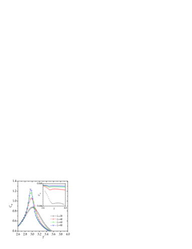
Figure 1 shows the heat capacity as function of $T$. A peak around $T\approx 2.94$, whose intensity increases with increasing lattice size, indicates the possibility of a phase transition at that temperature. As a first step, we analyze the behavior of the energy cumulant. It is well-known that the finite-size analysis of this quantity is a simple and direct way to determine the order of a phase transition Binder1984 ; Challa1986 ; Vilmayr1993 . The curves of $U_{H}$ versus $T$ are shown in the inset of Figure 1. It can clearly be observed that the minima in the energy cumulants tend to $2/3$ as the lattice size is increased. This behavior is typical of a continuous phase transition, because it indicates that the latent heat is zero in the thermodynamic limit.

Figure 1: Temperature dependence of the heat capacity and the energy cumulant (inset), for different lattice sizes as indicated.

Figure 2: Temperature dependence of the normalized magnetization and the Binder cumulant (inset), for different lattice sizes as indicated. Cumulants cross at around $T\approx 2.94$ and $U_{M}^{*}\approx 0.613$.

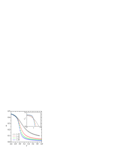
As it will be justified below, the normalized magnetization $m$ is a good parameter to study the magnetic order of the system. Although the ground state of the present model is not purely ferromagnetic, it can be shown that $m$ tends to a constant value: $\lim_{T\to 0}m=0.5$. In Figure 2 we show the temperature dependence of $m$ for different lattice sizes. In the inset, the corresponding Binder cumulants are presented, which intersect at around $T\approx 2.94$ and $U_{M}^{*}\approx 0.613$, confirming the existence of a finite-temperature continuous phase transition.

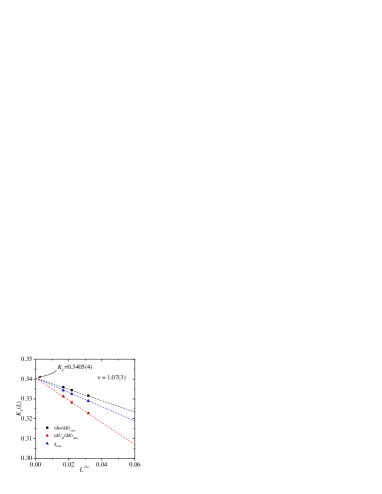
Furthermore, finite-size scaling theory BinderBook ; Fisher1971 ; Privman1990 allows for other efficient routes to estimate $T_{c}$ from the numerical data. One possible method, which is more accurate than the intersection of the Binder cumulant presented in the inset of Figure 2, relies on the extrapolation of the size-dependent inverse temperature, $K_{c}(L)$, to which different thermodynamic quantities reach their maximum values. Scaling theory predicts that

$$K_{c}(L)=K_{c}+{\rm const}.L^{-1/\nu}.$$ (15)

Among others, the maxima of the slopes of the order parameter and the Binder cumulant, $\left(dm/dK\right)_{\rm max}$ and $\left(dU_{M}/dK\right)_{\rm max}$, as well as of the susceptibility, $\chi_{\rm max}$, are quantities that can be used with this method. Performing a simultaneous fitting procedure using Eq. (15) and setting only two variables on the fit, i.e., $K_{c}$ and the exponent $\nu$, we obtain $K_{c}=0.3405(4)$ or $T_{c}=2.937(3)$, and $\nu=1.07(3)$. Figure 3 shows the corresponding plot of these quantities versus $L^{-1/\nu}$. Note that the critical temperature coincides, within numerical errors, with the value calculated from the crossing of the cumulants.

Figure 3: Size-dependent inverse temperature, $K_{c}(L)$, to which the maxima of the derivatives of the order parameter, $\left(dm/dK\right)_{\rm max}$, and the Binder cumulant, $\left(dU_{M}/dK\right)_{\rm max}$, as well as of the susceptibility, $\chi_{\rm max}$, reach their maximum values. Dashed lines correspond to fitting results.

Next, to calculate precise values for the critical exponents (including $\nu$), we make a conventional finite-size scaling analysis BinderBook ; Fisher1971 ; Privman1990 . At criticality, the finite-size scaling relations are

$$C_{H}=L^{\alpha/\nu}\widetilde{C}_{H}(L^{1/\nu}\epsilon)$$ (16)

$$m=L^{-\beta/\nu}\widetilde{m}(L^{1/\nu}\epsilon)$$ (17)

$$\chi=L^{\gamma/\nu}\widetilde{\chi}(L^{1/\nu}\epsilon)$$ (18)

$$U_{M}=\widetilde{U}_{M}(L^{1/\nu}\epsilon)$$ (19)

for $L\to\infty$, $\epsilon\to 0$ such that $L^{1/\nu}\epsilon$ = finite, where $\epsilon\equiv T/T_{c}-1$. Here, $\alpha$, $\beta$, $\gamma$ and $\nu$ are the standard critical exponents of the specific heat ($C_{H}\sim|\epsilon|^{-\alpha}$ for $\epsilon\to 0$, $L\to\infty$), order parameter ($m\sim-\epsilon^{\beta}$ for $\epsilon\to 0^{-}$, $L\to\infty$), susceptibility ($\chi\sim|\epsilon|^{\gamma}$ for $\epsilon\to 0$, $L\to\infty$) and correlation length $\xi$ ($\xi\sim|\epsilon|^{-\nu}$ for $\epsilon\to 0,L\to\infty$), respectively. $\widetilde{C}_{H}$, $\widetilde{m}$, $\widetilde{\chi}$ and $\widetilde{U}_{M}$ are scaling functions for the respective quantities.

Following the line of Refs. Ferrenberg1991 ; Janke1994 ; Binder2001 , the critical exponent $\nu$ is firstly computed by considering different derivatives with respect to the inverse temperature $K=1/T$, for example, the derivative of the Binder cumulant and the logarithmic derivative of the order parameter. It is expected that the maximum value of these derivatives as a function of the lattice size follows a power law of the form $\sim L^{1/\nu}$. Once the value of $\nu$ is known, the critical exponent $\gamma$ can be determined by scaling the maximum value of the susceptibility, i. e., from $\chi_{\mathrm{max}}\sim L^{\gamma/\nu}$. In addition, the standard way to extract the exponent $\beta$ is to study the scaling behavior of the order parameter at the point of inflection, $m_{\mathrm{inf}}$. We expect that $m_{\mathrm{inf}}\sim L^{-\beta/\nu}$. From this analysis we obtain $\nu=1.02(2)$, $\gamma/\nu=1.746(6)$, and $\beta/\nu=0.126(6)$, and then $\gamma=1.78(4)$ and $\beta=0.128(8)$. On the other hand, the maximum of the specific heat, $C_{H\mathrm{max}}$, does not follow a power law. Instead, we observe a logarithmic divergence of the form $C_{H\mathrm{max}}\approx 0.071+0.268\ln(L)$. This implies that the corresponding critical exponent is zero, $\alpha=0$ StanleyBook .

Figure 4: Data collapses for (a) the order parameter, (b) the Binder cumulant, (c) the susceptibility and (b) the heat capacity. Symbols are the same as in Figure 2.

We simulated system sizes only up to $L=80$, which gives probably the main contribution to the size of the error bars of the obtained critical exponents. Nevertheless, as the obtained values are compatible with those of the 2D Ising model, $\nu=1$, $\beta=1/8=0.125$, $\gamma=7/4=1.75$, and $\alpha=0$, we conclude that the observed phase transition probably belongs to this universality class. We should notice that $\nu=1.07(3)$, calculated from the simultaneous fitting to the Eq. (15), is very close to one but does not agree within error bars. This discrepancy may be due to the finite-size effects.

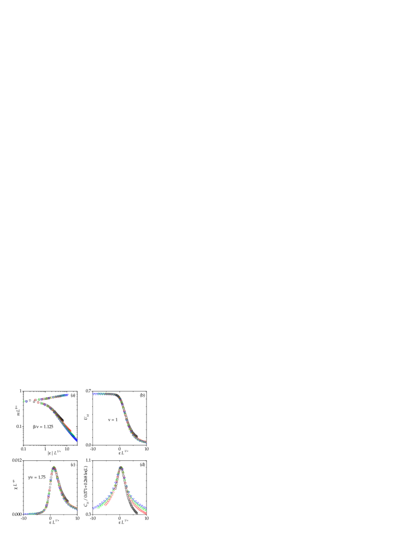
Figures 4 (a)-(d) show good data collapses for, respectively, the order parameter, the Binder cumulant, and the susceptibility where we use the Ising exponents (the data collapses do not change significantly if the exponents obtained numerically are used), while for the heat capacity we use the logarithmic correction term determined above. As we can see, we obtain very satisfactory scalings.

3.2 Bond structure and the ground-state properties

Figure 5: Mean fraction of frustrated plaquettes as function of $T$ for a lattice size $L=20$. Inset: Temperature derivative $df/dT$ for different lattice sizes as indicated.

In the previous subsection we have shown that the present model has a standard finite-temperature transition. We show here that the low-temperature equilibrium dynamics and the ground-state properties of the model present a rather interesting and rich behavior. To carried out the corresponding studies, we have performed additional simulations on smaller lattice sizes (ranging from $L=6$ to $L=20$) and for lower temperature, $T_{R}=0.1$.

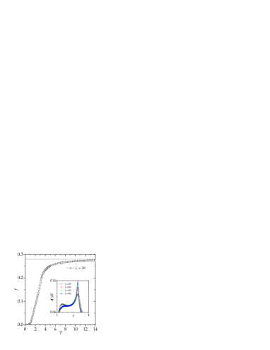
Figure 5 shows, for a system of lattice size $L=20$, the fraction of frustrated plaquettes, $f$, as function of $T$. For the limit $T\to\infty$ this fraction tends to a constant value of about $0.28$. In contrast, the Edwards-Anderson $\pm J$ model has a larger value $f=0.5$ (in this case, for any temperature). This shows that, even for the full-disordered state, the majority rule given by Eq. (2) induces strong correlations between bonds. On the other hand, for $T\to 0$ the model shows a non-frustrated ground state with $f=0$. What happens is that, at equilibrium, the dynamics efficiently eliminates any frustration.

In the inset of Figure 5 we can see the temperature derivative $df/dT$ for different lattice sizes. Because it is not possible to equilibrate large lattice sizes up to very low temperatures, these curves are only shown in the range of $T=1$ to $T=4$. As expected, $df/dT$ shows a size-dependent peak at approximately $T_{c}$, but another at $T\approx 1.4$ which for $L>20$ quickly leads to a characteristic knee feature. We can not associate the latter temperature to a critical one. Nevertheless, this is in the temperature range at which we observe the onset of the slow dynamics, as shown below.

A more complex behavior is displayed by the fractions of ferromagnetic and antiferromagnetic bonds, $p_{\mathrm{F}}$ and $p_{\mathrm{AF}}$, respectively. Figure 6 shows these quantities for $L=20$. It is observed in Figure 6 that when $T\to\infty$ the fractions of ferromagnetic and antiferromagnetic bonds reach a limiting constant value, with $p_{\mathrm{F}}>p_{\mathrm{AF}}$. Both limit values are easily calculated. The number of configurations of the spins surrounding a given pair is $2^{6}$. Two of them corresponds to all spins pointing in the same direction while in another twelve, one spin point in a direction opposite to the remaining (e. g., one spin up and the other down, or vice versa). The majority rule, Eq. (2), indicates that for these fourteen configurations the bond $J_{ij}$ is antiferromagnetic and otherwise is ferromagnetic. Then, considering that for $T\to\infty$ all configurations are equally likely, we obtain $\lim_{T\to\infty}p_{\mathrm{AF}}=14/2^{6}=0.21875$ and $\lim_{T\to\infty}p_{\mathrm{F}}=1-0.21875=0.78125$. Dotted lines in Figure 6 indicate these limit values.

Figure 6: The fractions of ferromagnetic and antiferromagnetic bonds $p_{\mathrm{F}}$ and $p_{\mathrm{AF}}$, respectively, as function of $T$. Dotted lines indicate the limit values of these quantities when $T\to\infty$. Inset shows the same curves at low temperatures.

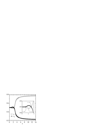
Furthermore, it can be observed in Figure 6 that for $T\to 0$ the system tends to a ground state with the same fractions of both types of bonds, $\lim_{T\to 0}p_{\mathrm{F}}=\lim_{T\to 0}p_{\mathrm{AF}}=0.5$. Interestingly enough, the inset shows that the fractions of ferromagnetic and antiferromagnetic bonds have a non-monotonous behavior in a finite temperature range. At $T\approx 2.3$ the curves of $p_{\mathrm{F}}$ and $p_{\mathrm{AF}}$ cross each other and, between this temperature and $T\approx 0.7$, the fraction of ferromagnetic bonds is smaller than $0.5$ and reaches a minimum at $T\approx 1.7$ (and of course, $p_{\mathrm{AF}}$ reaches its maximum). Then, for $T\lesssim 0.7$ both quantities are virtually identical. In what follows, we will always have in mind these particular temperatures when analyzing other observables.

Figure 7: Temperature dependence of the mean energy per spin for $L=20$. Inset shows the ground-state entropy as function of $1/N$.

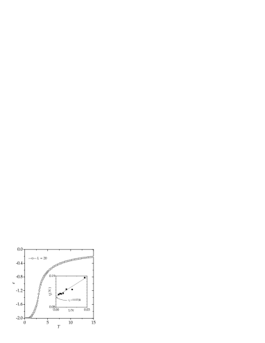
Although the ground state has an equal number of ferromagnetic and antiferromagnetic bonds, there are important differences between this system and the Edwards-Anderson $\pm J$ model. Figure 7 shows the mean energy as a function of $T$. We can see that this quantity tends to $-2$ at zero temperature, $e_{0}\equiv\lim_{T\to 0}e=-2$. This is a logical limit value since, as we have previously observed, the ground state is not frustrated. In contrast, the 2D Edwards-Anderson $\pm J$ model has a higher value of $e_{0}\approx-1.4$ Roma2004 .

We can obtain more information from the ground-state entropy per spin, $s_{0}$. In order to determine $s_{0}$, we have simulated the system between $T_{1}=300$ and $T_{R}=0.1$. Samples with $L\leq 20$ were used because only for these lattice sizes it is possible to achieve equilibrium at such low temperatures. The ground-state entropy per spin (in units of $k_{B}$) is calculated using the thermodynamic integration method Roma2004 ; Kirkpatrick1977 ; Binder1985 and is defined by the expression Perez2012

$$s_{0}(N)=\ln 2+\int_{e_{\infty}}^{e_{0}}\frac{\mathrm{d}e}{T},$$ (20)

where $e_{\infty}\equiv\lim_{T\to\infty}e=0$. Inset in Figure 7 shows $s_{0}(N)$ as function of $1/N$. Extrapolating, we obtain a thermodynamic limit value of $s_{0}\equiv\lim_{N\to\infty}s_{0}(N)=0.117(4)$. To extrapolate, only lattices with $L\geq 10$ were used because the entropy for smaller lattice sizes present some oscillations, which seem to be related to the periodic boundary conditions Perez2012 . This entropy value is larger than the corresponding one of the 2D Edwards-Anderson $\pm J$, $s_{0}^{\mathrm{EA}}\approx 0.07$ Perez2012 ; Saul1994 ; Zhan2000 ; Hartmann2001b . So that, our system has a non-frustrated and highly-degenerated ground state.

Figure 8: (a) Typical and (b) fully ordered ground-state configurations for lattice size $L=20$. Minority and majority spins are indicated by closed and open black circles, respectively, while ferromagnetic bonds are denoted by red lines (antiferromagnetic bonds are omitted for simplicity).

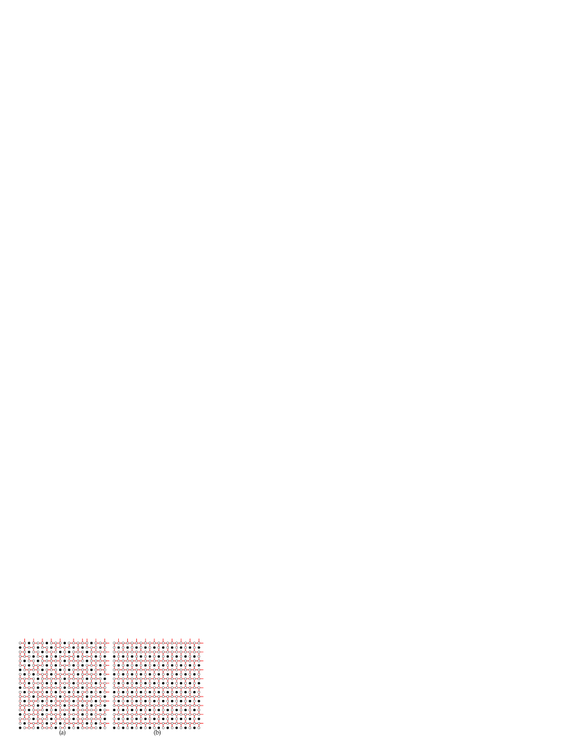
A better understanding of this phenomenon can be achieved by analyzing the structure of the ground state. The parallel-tempering algorithm can be used as a heuristic to obtain the lowest energy configurations Moreno2003 ; Roma2009 . We emphasize that for this application it is not necessary to reach equilibrium, because only configurations with $e=-2$ are sought. Figure 8 (a) shows a typical ground state. Analyzing many configurations like the one in Figure 8 (a), one can conceive that a fully ordered structure as the one shown in Figure 8 (b) might also be found in the ground-state. Although this latter configuration has energy $e=-2$ and is compatible with the majority rule, Eq. (2), it is extremely rare and is very unlikely to obtain using any algorithm.

Figure 9: Typical configurations for (a) $T=\infty$ and (b) $T=3.0$. Symbols are the same as in Figure 8.

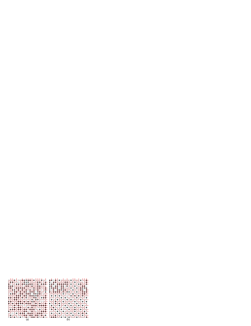
Such ground-state configurations have some interesting features. On one hand, we can see that a quarter of the spins (minority spins) point in a direction opposite to the remaining spins (majority spins). This is clearly related to the fact that $\lim_{T\to 0}m=0.5$ and the reason for using the magnetization $m$ as a good order parameter. More strictly, the ground state is not fully ferromagnetic but has a ferrimagnetic character. On the other hand, notice that minority spins have as nearest neighbors majority spins only, and these pairs are linked by antiferromagnetic bonds. Thus, in Figs. 8 (a) and (b) minority spins look as if they were isolated, i.e. minority spins do not interact among them.

Figure 10: (a) Spin correlation and (b) spin integrated response functions, at temperatures $T=2.9$, $2.3$, $1.0$, and $0.3$, and for different $t_{w}$ as indicated. Inset shows a zoom of the correlations functions for the two lower temperatures.

At infinite temperature all configurations are equally likely. Figure 9 (a) shows a typical high-temperature configuration, which has equal number of up and down spins (here, closed and open black circles represent, respectively, up and down spins). But, for a temperature close to the critical one, $T=3.0$, Figure 9 (b) shows that the “low-temperature phase” begins to develop [compare with Figures 8 (a) and (b)]. We can see that excitations are characterized by violations of the above features observed in the ground state (let us recall that, at $T=0$, minority spins have as nearest neighbors majority spins only, and these pairs are linked by antiferromagnetic bonds). For the particular temperatures indicated in the inset of Figure 6, in the range between $T=2.3$ and $T=0.7$, no anomaly is observed and all configurations are similar to those of the ground state.

Figure 11: FDT parametric plots $\rho(c)$ for the cases shown in Figs. 10 (a) and (b). Inset shows a zoom of the FDT plots for the two lower temperatures.

3.3 Out-of-equilibrium dynamic

At very low temperatures, it is numerically hard to reach equilibrium for large lattice sizes. In order to explore this region, we carry out extensive out-of-equilibrium simulations. Lattices of $L=200$ and six values of the waiting time, $t_{w}$ = 100, 200, 400, 800, and 1600, were used. For each temperature we have performed averages over $5000$ independent runs.

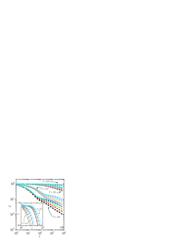
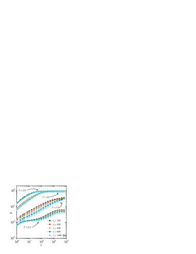
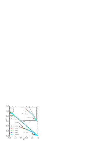
Figures 10 (a) and (b) show the spin correlation and spin integrated response functions for different temperatures. For temperatures $T=2.9$ (just below $T_{c}$) and $T=2.3$, above which $p_{\mathrm{F}}>p_{\mathrm{AF}}$, correlation functions tend to develop a plateau for increasing waiting time while response functions get stuck in a well defined plateau for all waiting times. When represented in a FDT parametric plot, as in Figure 11, this behavior leads to the typical coarsening-like violation of the FDT Crisanti2003 signaled by a constant $\rho(C)$ curve, highlighted with dotted lines in Figure 11. This would be the expected result for our model, which undergoes a thermodynamic continuous phase transition belonging to the 2D Ising universality class.

For a lower temperature $T=1.0$, all correlation and response functions curves in Figure 10 show a slightly different behavior which is more evident in Figure 11. In this case the FDT parametric plot seems to slowly converge to a FDT violation characterized by a finite slope at sufficiently long times, i.e. small values of $C$, although some curvature due to finite $t_{w}$ effects cannot be discarded. Interestingly, this FDT violation is reminiscent of the typical FDT violation found in mean-field models for structural glasses Crisanti2003 ; Berthier2011 , characterized by a one-step replica symmetry breaking Parisi2003 . This singular behavior is displayed within a wide temperature range around $T=1.0$, and is concomitant with the onset of the slow dynamics. On the other hand, even more surprising is the fact that upon further lowering the temperature, for $T=0.3$ the correlation functions show the emergence of a plateau close to $C=1$ and the response function also develops a plateau at a very small value, as shown in Figure 10. The result is a coarsening-like FDT violation as shown in Figure 11.

Figure 12: Temperature dependence of (a) the mean fraction of frustrated plaquettes and (b) the mean energy per spin. Both panels show the corresponding equilibrium and out-of-equilibrium curves for different times as indicated. Inset shows the same information for the mean fraction of ferromagnetic bonds.

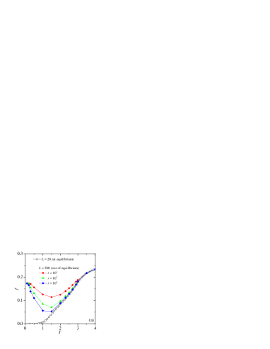
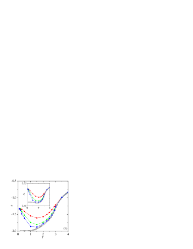
In order to shed some light on this phenomenon, we analyze again the bond structure but this time comparing thermal equilibrium with out-of-equilibrium measurements of the same observables. Figure 12 (a) shows the temperature dependence of the mean fraction of frustrated plaquettes comparing equilibrium with time-dependent measurements. The same comparison is shown in Figure 12 (b) and its inset for the mean energy per spin and the mean fraction of ferromagnetic bonds, respectively. From these figures some common features are revealed. For temperatures around the critical temperature $T_{c}$, all quantities rapidly relax to their equilibrium values [for long times there is not a perfect agreement between equilibrium and out-of-equilibrium values, because both calculations were performed for different lattice sizes, as indicated in the key of Figure 12 (a)]. Therefore, in this temperature range, for example at $T=2.9$ and $T=2.3$, the out-of-equilibrium dynamics is fast enough to develop a coarsening process, as noted in the analysis of the QFDT, Figure 11 above.

A different situation arises for $T\sim 1$, where for the studied time scales the dynamics is clearly slower and the system remains in a state with higher energy than expected at equilibrium. In this state, as can be observed in Figure 12 (a), the slow dynamics has not been effective in removing the frustration of the system. It is not surprising then that this dynamic and structural changes around $T\sim 1$ lead to a different QFDT characteristic, which in this case resembles the one observed in structural glasses.

Finally, at very small temperatures, Figs. 12 (a) and 12 (b) show that the very slow dynamics is not able to remove the frustration and the system is stuck in a high energy configuration. However, the values of mean fraction of frustrated plaquettes and mean energy per spin, let say for $T=0.3$, are very similar to those measured for temperatures close to $T_{c}$, let say $T=2.9$. Our interpretation is that for these values of frustration and energy the relaxation processes should be very similar and then we observe the characteristic coarsening feature in the QFDT at $T=0.3$, Figure 11. At such a small temperature the relaxation is so slow that a different relaxation mechanism at longer times can not be discarded only based on our numerical simulations.

4 Conclusions

In this work we have studied the critical behavior, the ground-state properties and the out-of-equilibrium dynamics of a 2D Ising model with non-static interactions. Its most important feature is that bonds are drawn according to a majority rule, Eq. (2), which was designed to prevent the system from ordering in full ferromagnetic or antiferromagnetic states. Nevertheless, we have demonstrated through equilibrium simulations, that the model has a low-temperature ferrimagnetic state and undergoes a continuous phase transition at $T_{c}=2.937(3)$, which probably belongs to the 2D Ising universality class.

The ground state is nontrivial. Although frustration is completely removed at $T=0$, (i. e. the energy per spin is $e_{0}=-2$) the ground state is highly degenerated with an entropy per spin of $s_{0}=0.117(4)$. Interactions form a degenerate structure where minority spins have as nearest neighbors majority spins only, and these pairs are linked by antiferromagnetic bonds.

This degenerate low-temperature phase has a low free energy and therefore is more stable than the one of the Ising model (which has a non-degenerate ground state). As a consequence, the critical temperature of the system, $T_{c}=2.937(3)$, is slightly larger than the one of the Ising ferromagnetic model, $T_{c}^{\mathrm{Ising}}\approx 2.269$ Onsager1944 .

In order to quantify this statement we use a free-energy minimization criterion Roma2003 . Let us consider a generic model undergoing a continuous phase transition. In the limits $T\to\infty$ and $T\to 0$ such a system is characterized by two extreme states: a fully-disordered (FD) state characterized, respectively, with an energy and an entropy per spin $e^{\prime}_{\mathrm{FD}}$ and $s^{\prime}_{\mathrm{FD}}$, and a fully-ordered (FO) state with the corresponding parameters $e^{\prime}_{\mathrm{FO}}$ and $s^{\prime}_{\mathrm{FO}}$. The Helmholtz free energy of these states are $f^{\prime}_{\mathrm{FD}}=e^{\prime}_{\mathrm{FD}}-Ts^{\prime}_{\mathrm{FD}}$ and $f^{\prime}_{\mathrm{FO}}=e^{\prime}_{\mathrm{FO}}-Ts^{\prime}_{\mathrm{FO}}$. The minimization criterion consists in considering that the critical behavior is mainly determined by the FD and FO states. Since in thermodynamic equilibrium the stable state corresponds to the minimum of the Helmholtz free energy, then

$$f^{\prime}_{\mathrm{FD}} < f^{\prime}_{\mathrm{FO}}\ \ \mathrm{if}\ T>T^{\prime}_{c}$$ (21)

$$f^{\prime}_{\mathrm{FD}} = f^{\prime}_{\mathrm{FO}}\ \ \mathrm{if}\ T=T^{\prime}_{c}$$ (22)

$$f^{\prime}_{\mathrm{FD}} > f^{\prime}_{\mathrm{FO}}\ \ \mathrm{if}\ T<T^{\prime}_{c}.$$ (23)

Finally, from Eq. (22) we can estimate the critical temperature as

$$T^{\prime}_{c}=\frac{\Delta e^{\prime}}{\Delta s^{\prime}},$$ (24)

where $\Delta e^{\prime}=e^{\prime}_{\mathrm{FD}}-e^{\prime}_{\mathrm{FO}}$ and $\Delta s^{\prime}=s^{\prime}_{\mathrm{FD}}-s^{\prime}_{\mathrm{FO}}$.

Our model and the Ising model have non-frustrated ground states and therefore $\Delta e=\Delta e^{\mathrm{Ising}}=2$. However, since for the FD state both systems have the same entropy, $s_{\mathrm{FD}}=s^{\mathrm{Ising}}_{\mathrm{FD}}=\ln 2$, but for the FO state $s_{\mathrm{FO}}>s^{\mathrm{Ising}}_{\mathrm{FO}}$=0, then their entropy changes are different, $\Delta s<\Delta s^{\mathrm{Ising}}=\ln 2$. Hence, from Eq. (24) we can determine that the critical temperatures will be $T_{c}>T_{c}^{\mathrm{Ising}}$. Note that the free-energy minimization criterion does not provide a good estimation of $T_{c}$, but it offers a very useful tool for understanding the critical behavior of a system with respect to parameter variations Roma2003 .

Finally, we have determined that the out-of-equilibrium dynamics has a novel behavior: at very low temperatures as well as near $T_{c}$ (but below of this critical temperature) we observed a coarsening-like FDT violation, while at an intermediate temperatures ($T\sim 1$) the FDT parametric plots are quite similar to those found for structural glasses. Nevertheless, for the latter case, note that in the parametric FDT plot the slope at sufficiently long times (FDT ratio) shows a small dependence on $t_{w}$, and therefore we cannot exclude that such phenomenon is due to finite-time effects. Comparing equilibrium with out-of-equilibrium measurements of different observables ($f$, $e$, and $p_{\mathrm{F}}$), we have been able to establish a connection between this phenomenon and the bond structure properties of the system.

O.A.P. acknowledges financial support from Universidad Nacional de Santiago del Estero, Argentina, under project CICyT-UNSE 23 A173. F.R. acknowledges financial support from CONICET (PIP 114-201001-00172) and Universidad Nacional de San Luis, Argentina (PROIPRO 3-1-0214) and thanks the LPTHE, France, for hospitality during the preparation of this work. S.B. is partially supported by CONICET (PIP11220090100051) and FONCyT (PICT2010-889).

References

- (1) K. Binder, A.P. Young, Rev. Mod. Phys. 58, 801 (1986).
- (2) M. E. J. Newman and C. Moore, Phys. Rev. E 60, 5068 (1999).
- (3) A. Lipowski, J. Phys. A 30, 7365 (1997).
- (4) M. R. Swift, H. Bokil, R. D. M. Travasso, and A. Bray, Phys. Rev. B 62, 11494 (2000).
- (5) A. Buhot and J. P. Garrahan, Phys. Rev. Lett. 88, 225702 (2002).
- (6) A Cavagna, I. Giardina, and T. S. Grigera, J. Chem. Phys. 118, 6974 (2003).
- (7) G. Biroli and M. Mezard, Phys. Rev. Lett. 88, 025501 (2001).
- (8) F. Krzakala, M. Tarzia, and L. Zdeborová, Phys. Rev. Lett. 101, 165702 (2008).
- (9) P. Lazić and D. K. Sunko, Eur. Phys. J. B 21, 595 (2001).
- (10) S.F. Edwards, P.W. Anderson, J. Phys. F: Met. Phys. 5, 965 (1975).
- (11) G.Toulouse, Commun.Phys. 2, 115 (1977).
- (12) A. K. Hartmann, Phys. Rev. B 67, 214404 (2003).
- (13) A. Fierro, Phys. Rev. E 70, 012501 (2004).
- (14) C. J. Geyer, Computing Science and Statistics: Proceedings of the 23rd Symposium on the Interface, American Statistical Association, New York, (1991) pag. 156.
- (15) K. Hukushima, K. Nemoto, Phys. Soc. Japan 65 (1996) 1604.
- (16) N. Metropolis, A. W. Rosenbluth, N. M. Rosenbluth, A. H. Teller, E. Teller, J. Chem. Phys. 21 (1953) 1087.
- (17) A. K. Hartmann and H. Rieger, Optimization Algorithms in Physics (Wiley-VCH, Berlin, 2001).
- (18) D. J. Earl and M. W. Deem, Phys. Chem. Chem. Phys. 7, 3910 (2005).
- (19) H. G. Katzgraber, S. Trebst, D. A. Huse, and M. Troyer, J. Stat. Mech.: Theory Exp. 2006, P03018 (2006).
- (20) D. P. Landau and K. Binder, A Guide to Monte Carlo Simulations in Statistical Physics, (Cambridge University Press, UK, 2005).
- (21) K. Binder, Applications of the Monte Carlo Method in Statistical Physics. Topics in current Physics, (Springer, Berlin, 1984), Vol. 36.
- (22) W. H. Press, S. A. Teukolsky, W. T. Vetterling, and B. P. Flannery, Numerical Recipes in C (Cambridge University Press, Cambridge, 1995).
- (23) C. Chatelain, J. Phys. A: Math. Gen. 36, 10739 (2003).
- (24) F. Ricci-Tersenghi, Phys. Rev. E 68, 065104R (2003).
- (25) L.F. Cugliandolo, J. Kurchan, J. Phys. A: Math. Gen. 27, 5749 (1994).
- (26) A. Crisanti, F. Ritort, J. Phys. A: Math. Gen. 36, R181 (2003).
- (27) H. G. Katzgraber, M. Körner, and A. P. Young, Phys. Rev. B 73, 224432 (2006).
- (28) K. Binder, D. P. Landau, Phys. Rev. B 30, 1477 (1984).
- (29) M.S.S. Challa, D.P. Landau, K. Binder, Phys. Rev. B 34, 1841 (1986).
- (30) K. Vollmayr, J.D. Reger, M. Scheucher, K. Binder, Z. Phys. B: Condens. Matter 91, 113 (1993).
- (31) M. E. Fisher, Critical Phenomena, (Academic Press, London, 1971).
- (32) V. Privman, Finite Size Scaling and Numerical Simulation of Statistical Systems, (World Scientific, Singapore, 1990).
- (33) A.M. Ferrenberg, D.P. Landau, Phys. Rev. B 44, 5081 (1991).
- (34) W. Janke, M. Katoot, R. Villanova, Phys. Rev. B 49, 9644 (1994).
- (35) K. Binder, E. Luijten, Physics Reports 344, 179 (2001).
- (36) H. E. Stanley, Introduction to Phase Transitions and Critical Phenomena, (Oxford University Press, New York, 1971).
- (37) F. Romá, F. Nieto, E. E. Vogel, and A. J. Ramirez-Pastor, J. Stat Phys. 114, 1325 (2004).
- (38) S. Kirkpatrick, Phys. Rev. B 16, 4630 (1977).
- (39) K. Binder, J. Comput. Phys. 59, 1 (1985).
- (40) D. J. Perez-Morelo, A. J. Ramirez-Pastor, and F. Romá., Physica A 391, 937 (2012).
- (41) K. Saul and M. Kardar, Nuclear Physics B 432, 641 (1994).
- (42) J. S. Zhan and L. W. Lee, Physica A 295, 239 (2000).
- (43) A. K. Hartmann, Phys. Rev. E 63, 016106 (2001).
- (44) J. L. Moreno, H. G. Katzgraber, and A. K. Hartmann, Int. J. Mod. Phys. C 14, 285 (2003).
- (45) F. Romá, S. Risau-Gusman, A. J. Ramirez-Pastor, F. Nieto, and E. E. Vogel, Physica A 388, 2821 (2009).
- (46) L. Berthier and G. Biroli, Rev. Mod. Phys. 83, 587 (2011).
- (47) G. Parisi, in Slow Relaxations and Nonequilibrium Dynamics in Condensed Matter, (Springer, Berlin, 2003).
- (48) L. Onsager, Phys. Rev. 65, 117 (1944).
- (49) F. Romá, A. J. Ramirez-Pastor, and J. L. Riccardo, Phys. Rev. B 68, 205407 (2003).