Rapid Sampling for Visualizations
with Ordering Guarantees

Abstract

Visualizations are frequently used as a means to understand trends and gather insights from datasets, but often take a long time to generate. In this paper, we focus on the problem of rapidly generating approximate visualizations while preserving crucial visual properties of interest to analysts. Our primary focus will be on sampling algorithms that preserve the visual property of ordering; our techniques will also apply to some other visual properties. For instance, our algorithms can be used to generate an approximate visualization of a bar chart very rapidly, where the comparisons between any two bars are correct. We formally show that our sampling algorithms are generally applicable and provably optimal in theory, in that they do not take more samples than necessary to generate the visualizations with ordering guarantees. They also work well in practice, correctly ordering output groups while taking orders of magnitude fewer samples and much less time than conventional sampling schemes.

1 Introduction

To understand their data, analysts commonly explore their datasets using visualizations, often with visual analytics tools such as Tableau [27] or Spotfire [47]. Visual exploration involves generating a sequence of visualizations, one after the other, quickly skimming each one to get a better understanding of the underlying trends in the datasets. However, when the datasets are large, these visualizations often take very long to produce, creating a significant barrier to interactive analysis.

Our thesis is that on large datasets, we may be able to quickly produce approximate visualizations of large datasets preserving visual properties crucial for data analysis. Our visualization schemes will also come with tuning parameters, whereby users can select the accuracy they desire, choosing less accuracy for more interactivity and more accuracy for more precise visualizations.

We show what we mean by “preserving visual properties” via an example. Consider the following query on a database of all flights in the US for the entire year:

${\tt Q:\ SELECT\ \ NAME,\ \ AVG(DELAY)\ \ FROM\ \ FLT\ \ GROUP\ \ BY\ \ NAME}$

The query asks for the average delays of flights, grouped by airline names. Figure 1 shows a bar chart illustrating an example query result. In our example, the average delay for AA (American Airlines) is 30 minutes, while that for JB (Jet Blue) is just 15 minutes. If the ${\tt FLT}$ table is large, the query above (and therefore the resulting visualization) is going to take a very long time to be displayed.

In this work, we specifically design sampling algorithms that generate visualizations of queries such as ${\tt Q}$, while sampling only a small fraction of records in the database. We focus on algorithms that preserve visual properties, i.e., those that ensure that the visualization appears similar to the same visualization computed on the entire database. The primary visual property we consider in this paper is the correct ordering property: ensuring that the groups or bars in a visualization or result set are ordered correctly, even if the actual value of the group differs from the value that would result if the entire database were sampled. For example, if the delay of JB is smaller than the delay of AA, then we would like the bar corresponding to JB to be smaller than the bar corresponding to AA in the output visualization. As long as the displayed visualizations obey visual properties (such as correct ordering), analysts will be able to view trends, gain insights, and make decisions—in our example, the analyst can decide which airline should receive the prize for airline with least delay, or if the analyst sees that the delay of AL is greater than the delay of SW, they can dig deeper into AL flights to figure out the cause for higher delay. Beyond correct ordering, our techniques can be applied to other visual properties, including:

• Accurate Trends: when generating line charts, comparisons between neighboring x-axis values must be correctly presented.

• Accurate Values: the values for each group in a bar chart must be within a certain bound of the values displayed to the analyst.

Figure 1: Flight Delays

We illustrate the challenges of generating accurate visualizations using our flight example. Here, we assume we have a sampling engine that allows us to retrieve samples from any airline group at a uniform cost per sample (we describe one such sampling engine we have built in Section 4.) Then, the amount of work done by any visualization generation algorithm is proportional to the number of samples taken in total across all groups. After performing some work (that is, after doing some sampling), let the current state of processing be depicted as in Figure 2, where the aggregate for each group is depicted using confidence intervals. Starting at this point, suppose we wanted to generate a visualization where the ordering is correct (like in Figure 1). One option is to use a conventional round-robin stratified sampling strategy [8], which is the most widely used technique in online approximate query processing [31, 30, 39, 28], to take one sample per group in each round, to generate estimates with shrinking confidence interval bounds. This will ensure that the eventual aggregate value of each group is roughly correct, and therefore that the ordering is roughly correct. We can in fact modify these conventional sampling schemes to stop once they are confident that the ordering is guaranteed to be correct. However, since conventional sampling is not optimized for ensuring that visual properties hold, such schemes will end up doing a lot more work than necessary (as we will see in the following).

A better strategy would be to focus our attention on the groups whose confidence intervals continue to overlap with others. For instance, for the data depicted in Figure 2, we may want to sample more from AA because its confidence interval overlaps with JB, AL, and SW while sampling more from UA (even though its confidence interval is large) is not useful because it gives us no additional information — UA is already clearly the airline with the largest delay, even if the exact value is slightly off. On the other hand, it is not clear if we should sample more from AA or DL, AA has a smaller confidence interval but overlaps with more groups, while DL has a larger confidence interval but overlaps with fewer groups. Overall, it is not clear how we may be able to meet our visual ordering properties while minimizing the samples acquired.

Figure 2: Flight Delays: Intermediate Processing

In this paper, we develop a family of sampling algorithms, based on sound probabilistic principles, that:

1. are correct, i.e., they return visualizations where the estimated averages are correctly ordered with a probability greater than a user-specified threshold, independent of the data distribution,

2. are theoretically optimal, i.e., no other sampling algorithms can take much fewer samples, and

3. are practically efficient, i.e., they require much fewer samples than the size of the datasets to ensure correct visual properties, especially on very large datasets. In our experiments, our algorithms give us reductions in sampling of up to 50X over conventional sampling schemes.

Our focus in this paper is on visualization types that directly correspond to a SQL aggregation query, e.g., a bar chart, or a histogram; these are the most commonly used visualization types in information visualization applications. While we also support generalizations to other visualization types (see Section 2.5), our techniques are not currently applicable to some visualizations, e.g., scatter-plots, stacked charts, timelines, or treemaps.

In addition, our algorithms are general enough to retain correctness and optimality when configured in the following ways:

1. Partial Results: Our algorithms can return partial results (that analysts can immediately peruse) improving gradually over time.

2. Early Termination: Our algorithms can take advantage of the finite resolution of visual display interfaces to terminate processing early. Our algorithms can also terminate early if allowed to make mistakes on estimating a few groups.

3. Generalized Settings: Our algorithms can be applied to other aggregation functions, beyond ${\tt AVG}$, as well as other, more complex queries, and also under more general settings.

4. Visualization Types: Our algorithms can be applied to the generation of other visualization types, such as trend-lines or chloropleth maps [49] instead of bar graphs.

2 Formal Problem Description

We begin by describing the type of queries and visualizations that we focus on for the paper. Then, we describe the formal problem we address.

2.1 Visualization Setting

Query: We begin by considering queries such as our example query in Section 1. We reproduce the query (more abstractly) here:

$Q:\ \ {\tt SELECT}\ \ X,\ \ {\tt AVG}(Y)\ \ {\tt FROM}\ \ R(X,\ \ Y)\ \ {\tt GROUP}\ \ {\tt BY}\ \ X$

This query can be translated to a bar chart visualization such as the one in Figure 1, where ${\tt AVG}(Y)$ is depicted along the $y-$axis, while $X$ is depicted along the $x-$axis. While we restrict ourselves to queries with a single GROUP BY and a AVG aggregate, our query processing algorithms do apply to a much more general class of queries and visualizations, including those with other aggregates, multiple group-bys, and selection or having predicates, as described in Section 2.5 (these generalizations still require us to have at least one ${\tt GROUP\ \ BY}$, which restricts us to aggregate-based visualizations, e.g., histograms, bar-charts, and trend-lines.

Setting: We assume we have an engine that allows us to efficiently retrieve random samples from $R$ corresponding to different values of $X$. Such an engine is easy to implement, if the relation $R$ is stored in main memory, and we have a traditional (B-tree, hash-based, or otherwise) index on $X$. We present an approach to implement this engine on disk in Section 4. Our techniques will also apply to the scenario when there is no index on $X$ in Section 6.3.6.

Notation: We denote the values that the group-by attribute $X$ can take as $x_{1}\ldots x_{k}$. We let $n_{i}$ be the number of tuples in $R$ with $X=x_{i}$. For instance, $n_{i}$ for $X=UA$ will denote the number of flights operated by $UA$ that year.

Let the $i$th group, denoted $S_{i}$, be the multiset of the $n_{i}$ values of $Y$ across all tuples in $R$ where $X=x_{i}$. In Figure 1, the group corresponding to $UA$ contains the set of delays of all the flights flown by $UA$ that year.

We denote the true averages of elements in a group $i$ as $\mu_{i}$: Thus, $\mu_{i}=\frac{\sum_{s\in S_{i}}s}{n_{i}}$. The goal for any algorithm processing the query $Q$ above is to compute and display $\mu_{i},\forall i\in 1\ldots k$, such that the estimates for $\mu_{i}$ are correctly ordered (defined formally subsequently).

Furthermore, we assume that each value in $S_{i}$ is bounded between $[0,c]$. For instance, for flights delays, we know that the values in $S_{i}$ are within [0, 24 hours], i.e., typical flights are not delayed beyond 24 hours. Note however, that our algorithms can still be used when no bound on $c$ is known, but may not have the desirable properties listed in Section 3.3.

2.2 Query Processing

Approach: Since we have an index on $X$, we can use the index to retrieve a tuple at random with any value of $X=x_{i}$. Thus, we can use the index to get an additional sample of $Y$ at random from any group $S_{i}$. Note that if the data is on disk, random access through a conventional index can be slow: however, we are building a system, called NeedleTail (also described in Section 4) that will address the problem of retrieving samples satisfying arbitrary conditions.

The query processing algorithms that we consider take repeated samples from groups $S_{i}$, and then eventually output estimates $\nu_{1},\ldots,$ $\nu_{k}$ for true averages $\mu_{1},\ldots,\mu_{k}$.

Correct Ordering Property: After retrieving a number of samples, our algorithm will have some estimate $\nu_{j}$ for the value of the actual average $\mu_{j}$ for each $j$. When the algorithm terminates and returns the eventual estimates $\nu_{1},\ldots\nu_{k}$, we want the following property to hold:

for all $i,j$ such that $\mu_{i}>\mu_{j}$, we have $\nu_{i}>\nu_{j}$

We desire that the query processing algorithm always respect the correct ordering property, but since we are making decisions probabilistically, there may be a (typically very small) chance that the output will violate the guarantee. Thus, we allow the analyst to specify a failure probability $\delta$ (which we expect to be very close to 0). The query processing scheme will then guarantee that with probability $1-\delta$, the eventual ordering is correct. We will consider other kinds of guarantees in Section 2.5.

2.3 Characterizing Performance

We consider three measures for evaluating the performance of query processing algorithms:

Sample Complexity: The cost for any additional sample taken by an algorithm from any of the groups is the same. We denote the total number of samples taken by an algorithm from group $i$ as $m_{i}$. Thus, the total sampling complexity of a query processing strategy (denoted ${\cal C}$) is the number of samples taken across groups:

$${\cal C}=\sum_{i\in 1\ldots k}m_{i}$$

Computational Complexity: While the total time will be typically dominated by the sampling time, we will also analyze the computation time of the query processing algorithm, which we denote ${\cal T}$.

Total Wall-Clock Time: In addition to the two complexity measures, we also experimentally evaluate the total wall-clock time of our query processing algorithms.

	Group 1		Group 2		Group 3		Group 4
1	[60, 90]	A	[20, 50]	A	[10, 40]	A	[40, 70]	A
…
20	[64, 84]	A	[28, 48]	A	[15, 35]	A	[45, 65]	A
21	[66, 84]	I	[30, 48]	A	[17, 35]	A	[46, 64]	A
…
57	[66, 84]	I	[32, 48]	A	[17, 33]	A	[46, 62]	A
58	[66, 84]	I	[32, 47]	A	[17, 32]	I	[46, 61]	A
…
70	[66, 84]	I	[40, 47]	A	[17, 32]	I	[46, 53]	A
71	[66, 84]	I	[40, 46]	I	[17, 32]	I	[47, 53]	I

Table 1: Example execution trace: active groups are denoted using the letter A, while inactive groups are denoted as I

2.4 Formal Problem

Our goal is to design query processing strategies that preserve the right ordering (within the user-specified accuracy bounds) while minimizing sample complexity:

Problem 1 (AVG-Order)

Given a query $Q$, and parameter values $c,\delta$, and an index on $X$, design a query processing algorithm returning estimates $\nu_{1},\ldots,\nu_{k}$ for $\mu_{1},\ldots,\mu_{k}$ which is as efficient as possible in terms of sample complexity ${\cal C}$, such that with probability greater than $1-\delta$, the ordering of $\nu_{1},\ldots,\nu_{k}$ with respect to $\mu_{1},\ldots,\mu_{k}$ is correct.

Note that in the problem statement we ignore computational complexity ${\cal T}$, however, we do want the computational complexity of our algorithms to also be relatively small, and we will demonstrate that for all algorithms we design, that indeed is the case.

One particularly important extension we cover right away is the following: visualization rendering algorithms are constrained by the number of pixels on the display screen, and therefore, two groups whose true average values $\mu_{i}$ are very close to each other cannot be distinguished on a visual display screen. Can we, by relaxing the correct ordering property for groups which are very close to each other, get significant improvements in terms of sample and total complexity? We therefore pose the following problem:

Problem 2 (AVG-Order-Resolution)

Given a query $Q$, and values $c,\delta$, a minimum resolution $r$, and an index on $X$, design a query processing algorithm returning estimates $\nu_{1},\ldots,\nu_{k}$ for $\mu_{1},\ldots,\mu_{k}$ which is as efficient as possible in terms of sample complexity ${\cal C}$, such that with probability greater than $1-\delta$, the ordering of $\nu_{1},\ldots,\nu_{k}$ with respect to $\mu_{1},\ldots,\mu_{k}$ is correct, where correctness is now defined as the following:

for all $i,j,i\neq j$, if $|\mu_{i}-\mu_{j}|\leq r$, then ordering $\nu_{i}$ before or after $\nu_{j}$ are both correct, while if $|\mu_{i}-\mu_{j}|>r$, then $\nu_{i}<\nu_{j}$ if $\mu_{i}<\mu_{j}$ and vice versa.

The problem statement says that if two true averages, $\mu_{i},\mu_{j}$ satisfy $|\mu_{i}-\mu_{j}|\leq r$, then we are no longer required to order them correctly with respect to each other.

2.5 Extensions

In Section 6 we discuss other problem variants:

• Ensuring that weaker properties hold:

  • Trends and Chloropleths: When drawing trend-lines and heat maps (i.e., chloropleths [49]), it is more important to ensure order is preserved between adjacent groups than between all groups.

  • Top-t Results: When the number of groups to be depicted in the visualization is very large, say greater than 20, it is impossible for users to visually examine all groups simultaneously. Here, the analyst would prefer to view the top-$t$ or bottom-$t$ groups in terms of actual averages.

  • Allowing Mistakes: If the analyst is fine with a few mistakes being made on a select number of groups (so that that the results can be produced faster), this can be taken into account in our algorithms.

• Ensuring that stronger properties hold:

  • Values: We can modify our algorithms to ensure that the averages $\nu_{i}$ for each group are close to the actual averages $\mu_{i}$, in addition to making sure that the ordering is correct.

  • Partial Results: We can modify our algorithms to return partial results as an when they are computed. This is especially important when the visualization takes a long time to be computed, so that the analyst to start perusing the visualization as soon as possible.

• Tackling other queries or settings:

  • Other Aggregations: We can generalize our techniques for aggregation functions beyond ${\tt AVG}$, including ${\tt SUM}$ and ${\tt COUNT}$.

  • Selection Predicates: Our techniques apply equally well when we have WHERE or HAVING predicates in our query.

  • Multiple Group Bys or Aggregations: We can generalize our techniques to handle the case where we are visualizing multiple aggregates simultaneously, and when we are grouping by multiple attributes at the same time (in a three dimensional visualization or a two dimensional visualization with a cross-product on the x-axis).

  • No indexes: Our techniques also apply to the scenario when we have no indexes.

Data: $S_{1},\ldots,S_{k},\delta$

1 Initialize $m\leftarrow 1$;

2 Draw $m$ samples from each of $S_{1},\ldots,S_{k}$ to provide initial estimates $\nu_{1},\ldots,\nu_{k}$;

3 Initialize $A=\{1,\ldots,k\}$;

4 while $A\neq\emptyset$ do

5       $m\leftarrow m+1$;

6       $\varepsilon=c\,\sqrt{(1-\frac{m/\kappa-1}{\max_{i\in A}n_{i}})\frac{2\log\log_{\kappa}(m)+\log(\pi^{2}k/3\delta)}{2m/\kappa}}$ /$\ast$Update Confidence Interval Size^† $\ast$/;

7       for each $i\in A$ do

8             Draw a sample $x$ from $S_{i}$;

9             $\nu_{i}\leftarrow\frac{m-1}{m}\nu_{i}+\frac{1}{m}x$;

10            

11      for each $i\in A$ do

12             if $[\nu_{i}-\varepsilon,\nu_{i}+\varepsilon]\cap\big{(}\bigcup_{j\in A\setminus\{i\}}[\nu_{j}-\varepsilon,\nu_{j}+\varepsilon]\big{)}=\emptyset$ then

13                  $A\leftarrow A\setminus\{i\}$

14            

15      

16Return $\nu_{1},\ldots,\nu_{k}$;

Algorithm 1 IFocus

3 The algorithm and its analysis

In this section, we describe our solution to Problem 1. We start by introducing the new IFocus algorithm in Section 3.1. We will analyze its sample complexity and demonstrate its correctness in Section 3.3. We will then analyze its computational complexity in Section 3.4. Finally, we will demonstrate that the IFocus algorithm is essentially optimal, i.e., no other algorithm can give us a sample complexity much smaller than IFocus, in Section 3.5.

3.1 The Basic IFocus Algorithm

The IFocus algorithm is shown in Algorithm 1. We describe the pseudocode and illustrate the execution on an example below.

At a high level, the algorithm works as follows. For each group, it maintains a confidence interval (described in more detail below) within which the algorithm believes the true average of each group lies. The algorithm then proceeds in rounds. The algorithm starts off with one sample per group to generate initial confidence intervals for the true averages $\mu_{1},\ldots,\mu_{k}$. We refer to the groups whose confidence intervals overlap with other groups as active groups. Then, in each round, for all the groups whose confidence intervals still overlap with confidence intervals of other groups, i.e., all the active groups, a single additional sample is taken. We terminate when there are no remaining active groups and then return the estimated averages $\nu_{1},\ldots,\nu_{k}$. We now describe an illustration of the algorithm on an example.

$k$	Number of groups.
$n_{1},\ldots,n_{k}$	Number of elements in each group.
$S_{1},\ldots,S_{k}$	The groups themselves. $S_{i}$ is a set of $n_{i}$ elements from $[0,1]$.
$\mu_{1},\ldots,\mu_{k}$	Averages of the elements in each group. $\mu_{i}=\operatorname*{\mathrm{E}}_{x\in S_{i}}[x]$.
$\tau_{i,j}$	Distance between averages $\mu_{i}$ and $\mu_{j}$. $\tau_{i,j}=|\mu_{i}-\mu_{j}|$.
$\eta_{i}$	Minimal distance between $\mu_{i}$ and the other averages. $\eta_{i}=\min_{j\neq i}\tau_{i,j}$.
$r$	Minimal resolution, $0\leq r\leq 1$.
$\eta_{i}^{(r)}$	Thresholded minimal distance; $\eta_{i}^{(r)}=\max\{\eta_{i},r\}$.

Table 2: Table of Notation

Example 3.1

An example of how the algorithm works is given in Table 1. Here, there are four groups, i.e., $k=4$. Each row in the table corresponds to one phase of sampling. The first column refers to the total number of samples that have been taken so far for each of the active groups (we call this the number of the round). The algorithm starts by taking one sample per group to generate initial confidence intervals: these are displayed in the first row.

At the end of the first round, all four groups are active since for every confidence interval, there is some other confidence interval with which it overlaps. For instance, for group 1, whose confidence interval is [60, 90], this confidence interval overlaps with the confidence interval of group 4; therefore group $1$ is active.

We “fast-forward” to round 20, where once again all groups are still active. Then, on round 21, after an additional sample, the confidence interval of group 1 shrinks to [66, 84], which no longer overlaps with any other confidence interval. Therefore, group 1 is no longer active, and we stop sampling from group 1. We fast-forward again to round 58, where after taking a sample, group 3’s confidence interval no longer overlaps with any other group’s confidence interval, so we can stop sampling it too. Finally, at round 71, none of the four confidence intervals overlaps with any other. Thus, the total cost of the algorithm (i.e., the number of samples) is

$${\cal C}=21\times 4+(58-21)\times 3+(71-58)\times 2$$

The expression $21\times 4$ comes from the 21 rounds when all four groups are active, $(58-21)\times 3$ comes from the rounds from 22 to 58, when only three groups are active, and so on.

The pseudocode for the algorithm is shown in Algorithm 1; $m$ refers to the round. We start at the first round (i.e., $m=1$) drawing one sample from each of $S_{1},\ldots,S_{k}$ to get initial estimates of $\nu_{1},\ldots,\nu_{k}$. Initially, the set of active groups, $A$, contains all groups from $1$ to $k$. As long as there are active groups, in each round, we take an additional sample for all the groups in $A$, and update the corresponding $\nu_{i}$. Based on the number of samples drawn per active group, we update $\varepsilon$, i.e., the half-width of the confidence interval. Here, the confidence interval $[\nu_{i}-\varepsilon,\nu_{i}+\varepsilon]$ refers to the $1-\delta$ confidence interval on taking $m$ samples, i.e., having taken $m$ samples, the probability that the true average $\mu_{i}$ is within $[\nu_{i}-\varepsilon,\nu_{i}+\varepsilon]$ is greater than $1-\delta$. As we show below, the confidence intervals are derived using a variation of Hoeffding’s inequality.

Discussion: We note several features of the algorithm:

• As we will see, the sampling complexity of IFocus does not depend on the number of elements in each group, and simply depends on where the true averages of each group are located relative to each other. We will show this formally in Section 3.3.

• The algorithm has similar guarantees and properties when the sampling per group is done with as against without replacement. We will discuss these differences in Section 3.6.

• There is a corner case that needs to be treated carefully: there is a small chance that a group that was not active suddenly becomes active because the average $\nu_{i}$ of some other group moves excessively due to the addition of a very large (or very small) element. We have two alternatives at this point

  • a) ignore the newly activated group; i.e., groups can never be added back to the set of active groups

  • b) allow inactive groups to become active.

  It turns out the properties we prove for the algorithm in terms of optimality of sample complexity (see Section 3.3) hold if we do a). If we do b), the properties of optimality no longer hold.

3.2 Proof of Correctness

We now prove that IFocus obeys the ordering property with probability greater than $1-\delta$. Our proof involves three steps:

• Step 1: The algorithm IFocus  obeys the correct ordering property, as long as the confidence intervals of each active group contain the actual average, during every round.

• Step 2: The confidence intervals of any given active group contains the actual average of that group with probability greater than $(1-\delta/k)$ at every round, as long as $\varepsilon$ is set according to Line 6 in Algorithm 1.

• Step 3: The confidence intervals of all active groups contains actual averages for the groups with probability greater than $(1-\delta)$ at every round, when $\varepsilon$ is set as per Line 6 in Algorithm 1.

Combining the three steps together give us the desired result.

Step 1: To complete this step, we need a bit more notation. For every $m>1$, let $A_{m}$, $\varepsilon_{m}$, and $\nu_{1,m},\ldots,\nu_{k,m}$ denote the values of $A,\varepsilon,\nu_{1},\ldots,\nu_{k}$ at step 10 in the algorithm for the iteration of the loop corresponding to $m$. Also, for $i=1,\ldots,k$, recall that $m_{i}$ is the number of samples required to estimate $\nu_{i}$; equivalently, it will denote the value of $m$ when $i$ is removed from $A$. We define $m_{max}$ to be the largest $m_{i}$.

Lemma 1

If for every $m\in 1\ldots m_{max}$ and every $j\in A_{m}$, we have $|\nu_{j,m}-\mu_{j}|\leq\varepsilon_{m}$, then the estimates $\nu_{1},\ldots,\nu_{k}$ returned by the algorithm have the same order as $\mu_{1},\ldots,\mu_{k}$, i.e., the algorithm satisfies the correct ordering property.

That is, as long as all the estimates for the active groups are close enough to their true average, that is sufficient to ensure overall correct ordering.

Proof 3.1.

Fix any $i\neq j\in\{1,\ldots,k\}$. We will show that $\nu_{i}>\nu_{j}$ iff $\mu_{i}>\mu_{j}$. Applying this to all $i,j$ gives us the desired result.

Assume without loss of generality (by relabeling $i$ and $j$, if needed) that $m_{i}\leq m_{j}$. Since $m_{i}\leq m_{j}$, $j$ is removed from the active groups at a later stage than $i$. At $m_{i}$, we have that the confidence interval for group $i$ no longer overlaps with other confidence intervals (otherwise $i$ would not be removed from the set of active groups). Thus, the intervals $[\nu_{i,m_{i}}-\varepsilon_{m_{i}},\nu_{i,m_{i}}+\varepsilon_{m_{i}}]$ and $[\nu_{j,m_{i}}-\varepsilon_{m_{i}},\nu_{j,m_{i}}+\varepsilon_{m_{i}}]$ are disjoint. Consider the case when $\mu_{i}<\mu_{j}$. Then, we have:

$$\mu_{i}\leq\nu_{i,m_{i}}+\varepsilon_{m_{i}} <\nu_{j,m_{i}}-\varepsilon_{m_{i}}\leq\mu_{j}$$ (1)

$$\implies\nu_{i,m_{i}} <\mu_{j}-\varepsilon_{m_{i}}$$ (2)

The first and last inequality holds because $\mu_{i}$ and $\mu_{j}$ are within the confidence interval around $\nu_{i}$ and $\nu_{j}$ respectively at round $m_{i}$. The second inequality holds because the intervals are disjoint. (To see this, notice that if the inequality was reversed, the intervals would no longer be disjoint.) Then, we have:

$$\nu_{j}=\nu_{j,m_{j}}\geq\mu_{j}-\varepsilon_{m_{j}}\geq\mu_{j}-\varepsilon_{m_{i}}>\nu_{i,m_{i}}=\nu_{i}.$$ (3)

The first equality holds because group $j$ exits the set of active groups at $m_{j}$; the second inequality holds because the confidence interval at $j$ contains $\mu_{j}$; the third inequality holds because $\varepsilon_{j}\leq\varepsilon_{i}$ (since confidence intervals shrink as the rounds proceed); the next inequality holds because of Equation 2; while the last equality holds because group $i$ exits the set of active groups at $m_{i}$. Therefore, we have $\nu_{i}<\nu_{j}$, as desired. The case where $\mu_{i}>\mu_{j}$ is essentially identical: in this case Equation 1 is of the form:

$$\mu_{i}\geq\nu_{i,m_{i}}-\varepsilon_{m_{i}}>\nu_{j,m_{i}}+\varepsilon_{m_{i}}\geq\mu_{j}$$

and Equation 3 is of the form:

$$\nu_{j}=\nu_{j,m_{j}}\leq\mu_{j}+\varepsilon_{m_{j}}\leq\mu_{j}+\varepsilon_{m_{i}}<\nu_{i,m_{i}}=\nu_{i}.$$

so that we now have $\nu_{i}>\nu_{j}$, once again as desired.

Step 2: In this step, our goal is to prove that the confidence interval of any group contains the actual average with probability greater than $(1-\delta/k)$ on following Algorithm 1.

For this proof, we use a specialized concentration inequality that is derived from Hoeffding’s classical inequality [50]. Hoeffding [29] showed that his inequality can be applied to this setting to bound the deviation of the average of random numbers sampled from a set from the true average of the set. Serfling [46] refined the previous result to give tighter bounds as the number of random numbers sampled approaches the size of the set.

Lemma 3.2 (Hoeffding–Serfling inequality [46]).

Let $\mathcal{Y}=y_{1},$ $\ldots,$ $y_{N}$ be a set of $N$ values in $[0,1]$ with average value $\frac{1}{N}\sum_{i=1}^{N}y_{i}=\mu$. Let $Y_{1},\ldots,Y_{N}$ be a sequence of random variables drawn from $\mathcal{Y}$ without replacement. For every $1\leq k<N$ and $\varepsilon>0$,

$$\Pr\left[\max_{k\leq m\leq N-1}\left|\frac{\sum_{i=1}^{m}Y_{i}}{m}-\mu\right|\geq\varepsilon\right]\leq 2\exp\left(-\frac{2k\varepsilon^{2}}{1-\frac{k-1}{N}}\right).$$

We use the above inequality to get tight bounds for the value of $\sum_{i=1}^{m}Y_{i}/m$ for all $1\leq m\leq N$, with probability $\delta$. We discuss next how to apply the theorem to complete Step 2 of our proof.

Theorem 3.2.

Let $\mathcal{Y}=y_{1},$ $\ldots,$ $y_{N}$ be a set of $N$ values in $[0,1]$ with average value $\frac{1}{N}\sum_{i=1}^{N}y_{i}=\mu$. Let $Y_{1},\ldots,Y_{N}$ be a sequence of random variables drawn from $\mathcal{Y}$ without replacement. Fix any $\delta>0$ and $\kappa>1$. For $1\leq m\leq N-1$, define

$$\varepsilon_{m}=\sqrt{\frac{(1-\frac{m/\kappa-1}{N})(2\log\log_{\kappa}(m)+\log(\pi^{2}/3\delta))}{2m/\kappa}}.$$

$$\text{Then:}\ \Pr\left[\exists m,1\leq m\leq N:\left|\frac{\sum_{i=1}^{m}Y_{i}}{m}-\mu\right|>\varepsilon_{m}\right]\leq\delta.$$

Proof 3.3.

We have:

$$\Pr\left[\exists m,1\leq m\leq N:\left|\frac{\sum_{i=1}^{m}Y_{i}}{m}-\mu\right|>\varepsilon_{m}\right]$$

$$\leq\sum_{r\geq 1}\Pr\left[\exists m,\kappa^{r-1}\leq m\leq\kappa^{r}:\left|\frac{\sum_{i=1}^{m}Y_{i}}{m}-\mu\right|>\varepsilon_{m}\right]$$

$$\leq\sum_{r\geq 1}\Pr\left[\exists m,\kappa^{r-1}\leq m\leq\kappa^{r}:\left|\frac{\sum_{i=1}^{m}Y_{i}}{m}-\mu\right|>\varepsilon_{\kappa^{r}}\right]$$

$$\leq\sum_{r\geq 1}\Pr\left[\max_{\kappa^{r-1}\leq m\leq N-1}\left|\frac{\sum_{i=1}^{m}Y_{i}}{m}-\mu\right|>\varepsilon_{\kappa^{r}}\right].$$

The first inequality holds by the union bound [50] (i.e., the probability that a union of events occurs is bounded above by sum of the probabilities that each occurs). The second inequality holds because $\varepsilon_{m}$ only decreases as $m$ increases. The third inequality holds because the condition that any of the sums on the left-hand side is greater than $\varepsilon_{\kappa^{r}}$ occurs when the maximum is greater than $\varepsilon_{\kappa^{r}}$.

By the Hoeffding–Serfling inequality (i.e., Lemma 3.2),

$$\Pr\left[\max_{\kappa^{r-1}\leq m\leq N-1}\left|\frac{\sum_{i=1}^{m}Y_{i}}{m}-\mu\right|>\varepsilon_{\kappa^{r}}\right]\leq\frac{6\delta}{\pi^{2}r^{2}}.$$

The theorem the follows from the identity $\sum_{r\geq 1}\frac{1}{r^{2}}=\pi^{2}/6$.

Now, when we apply Theorem 3.2 to any group $i$ in Algorithm 1, with $\varepsilon_{m}$ set as described in Line 6 in the algorithm, $N$ set to $n_{i}$, $Y_{i}$ being equal to the $i$th sample from the group (taken without replacement), and $\delta$ set to $\delta/k$, we have the following corollary.

Corollary 3.4.

For any group $i$, across all rounds of Algorithm 1, we have: $\Pr\left[\exists m,1\leq m\leq m_{i}:\left|\nu_{i,m}-\mu\right|>\varepsilon_{m}\right]\leq\delta/k.$

Step 3: On applying the union bound [50] to Corollary 3.4, we get the following result:

Corollary 3.5.

Across all groups and rounds of Algorithm 1: $\Pr\left[\exists i,m,1\leq i\leq k,1\leq m\leq m_{i}:\left|\nu_{i,m}-\mu\right|>\varepsilon_{m}\right]\leq\delta.$

This result, when combined with Lemma 1, allows us to infer the following theorem:

Theorem 3.5 (Correct Ordering).

The eventual estimates $\nu_{1},\ldots,\nu_{k}$ returned by Algorithm 1 have the same order as $\mu_{1},\ldots,\mu_{k}$ with probability greater than $1-\delta$.

3.3 Sample Complexity of IFocus

To state and prove the theorem about the sample complexity of IFocus, we introduce some additional notation which allows us to describe the “hardness” of a particular input instance. (Table 2 describes all the symbols used in the paper.) We define $\eta_{i}$ to be the minimum distance between $\mu_{i}$ and the next closest average, i.e., $\eta_{i}=\min_{j\neq i}{|\mu_{i}-\mu_{j}|}$. The smaller $\eta_{i}$ is, the more effort we need to put in to ensure that the confidence interval estimates for $\mu_{i}$ are are small enough compared to $\eta_{i}$.

In this section, we prove the following theorem:

Theorem 3.5 (Sample Complexity).

With probability at least $1-\delta$, IFocus  outputs estimates $\nu_{1},\ldots,\nu_{k}$ that satisfy the correct ordering property and, furthermore, draws

$$O\left(c^{2}\sum_{i=1}^{k}\frac{\log(\frac{k}{\delta})+\log\log(\frac{1}{\eta_{i}})}{\eta_{i}^{\,2}}\right)\ \text{samples in total.}$$ (4)

The theorem states that IFocus obeys the correct ordering property while drawing a number of samples from groups proportional to the sum of the inverse of the squares of the $\eta_{i}$: that is, the smaller the $\eta_{i}$, the larger the amount of sampling we need to do (with quadratic scaling).

The next lemma gives us an upper bound on how large $m_{i}$ can be in terms of the $\eta_{i}$, for each $i$: this allows us to establish an upper bound on the sample complexity of the algorithm.

Lemma 3.6.

Fix $i\in 1\ldots k$. Define $m_{i}^{*}$ to be the minimal value of $m\geq 1$ for which $\varepsilon_{m}<\eta_{i}/4$. In the running of the algorithm, if for every $j\in A_{m_{i}^{*}}$, we have $|\nu_{j,m_{i}^{*}}-\mu_{j}|\leq\varepsilon_{m_{i}^{*}}$, then $m_{i}\leq m_{i}^{*}$.

Intuitively, the lemma allows us to establish that $m_{i}<m_{i}^{*}$, the latter of which (as we show subsequently) is dependent on $\eta_{i}$.

Proof 3.7.

If $i\notin A_{m_{i}^{*}}$, then the conclusion of the lemma trivially holds, because $m_{i}<m_{i}^{*}$. Consider now the case where $i\in A_{m_{i}^{*}}$. We now prove that $m_{i}=m_{i}^{*}$. Note that $m_{i}=m_{i}^{*}$ if and only if the interval $[\nu_{i,m_{i}^{*}}-\varepsilon_{m_{i}^{*}},\nu_{i,m_{i}^{*}}+\varepsilon_{m_{i}^{*}}]$ is disjoint from the union of intervals $\bigcup_{j\in A_{m_{i}^{*}}\setminus\{i\}}[\nu_{j,m_{i}^{*}}-\varepsilon_{m_{i}^{*}},\nu_{j,m_{i}^{*}}+\varepsilon_{m_{i}^{*}}]$.

We focus first on all $j$ where $\mu_{j}<\mu_{i}$. By the definition of $\eta_{i}$, every $j\in A_{m_{i}^{*}}$ for which $\mu_{j}<\mu_{i}$ satisfies the stronger inequality $\mu_{j}\leq\mu_{i}-\eta_{i}$. By the conditions of the lemma (i.e., that confidence intervals always contain the true average), we have that $\mu_{j}\geq\nu_{j,m_{i}^{*}}-\varepsilon_{m_{i}^{*}}$ and that $\mu_{i}\leq\nu_{i,m_{i}^{*}}+\varepsilon_{m_{i}^{*}}$. So we have:

$$\nu_{j,m_{i}^{*}}+\varepsilon_{m_{i}^{*}}\leq\mu_{j}+2\varepsilon_{m_{i}^{*}}<\mu_{j}+\frac{\eta_{i}}{2}\leq\mu_{i}-\frac{\eta_{i}}{2}<\mu_{i}-2\varepsilon_{m_{i}^{*}}\leq\nu_{i,m_{i}^{*}}-\varepsilon_{m_{i}^{*}}$$

• The first and last inequalities follow the fact that the confidence interval for $\nu_{j}$ always contains $\mu_{j}$, i.e., $\mu_{j}\geq\nu_{j,m_{i}^{*}}-\varepsilon_{m_{i}^{*}}$;

• the second and fourth follow from the fact that $\varepsilon_{m_{i}^{*}}<\eta_{i}/4$;

• and the third follows from the fact that $\mu_{j}\leq\mu_{i}-\eta_{i}$.

Thus, the intervals $[\nu_{i,m_{i}^{*}}-\varepsilon_{m_{i}^{*}},\nu_{i,m_{i}^{*}}+\varepsilon_{m_{i}^{*}}]$ and $[\nu_{j,m_{i}^{*}}-\varepsilon_{m_{i}^{*}},\nu_{j,m_{i}^{*}}+\varepsilon_{m_{i}^{*}}]$ are disjoint. Similarly, for all $j\in A_{m_{i}^{*}}$ that satisfies $\mu_{j}>\mu_{i}$, we observe that the interval $[\nu_{i,m_{i}^{*}}-\varepsilon_{m_{i}^{*}},\nu_{i,m_{i}^{*}}+\varepsilon_{m_{i}^{*}}]$ is also disjoint from $[\nu_{j,m_{i}^{*}}-\varepsilon_{m_{i}^{*}},\nu_{j,m_{i}^{*}}+\varepsilon_{m_{i}^{*}}]$.

We are now ready to complete the analysis of the algorithm.

Proof 3.8 (of Theorem 3.5).

First, we note that for $i=1,\ldots,k$, the value $m_{i}^{*}$ is bounded above by

$$m_{i}^{*}=O\left(c^{2}\frac{\log\log\frac{1}{\eta_{i}^{\,2}}+\log\frac{k}{\delta}}{\eta_{i}^{\,2}}\right).$$

(To verify this fact, note that when $m=\frac{8c^{2}}{\eta_{i}^{\,2}}(\log\frac{\pi^{2}k}{3\delta}+\log\log\frac{8}{\eta_{i}{\,2}}+1)$, then the corresponding value of $\varepsilon$ satisfies $\varepsilon_{m}<\frac{\eta_{i}}{4}$.)

By Corollary 3.5, with probability at least $1-\delta$, for every $i\in 1,\ldots,k$, every $m\geq 1$, and every $j\in A_{m}$, we have $|\nu_{j,m}-\mu_{j}|\leq\varepsilon_{m}$. Therefore, by Lemma 1 the estimates $\nu_{1},\ldots,\nu_{k}$ returned by the algorithm satisfy the correct ordering property. Furthermore, by Lemma 3.6, the total number of samples drawn from the $i$th group by the algorithm is bounded above by $m_{i}^{*}$ and the total number of samples requested by the algorithm is bounded above by

$$\sum_{i=1}^{k}m_{i}^{*}=O\left(c^{2}\sum_{i=1}^{k}\frac{\log(\frac{k}{\delta})+\log\log(\frac{1}{\eta_{i}})}{\eta_{i}^{\,2}}\right).$$

We have the desired result.

3.4 Computational Complexity

The computational complexity of the algorithm is dominated by the check used to determine if a group is still active. This check can be done in $O(\log|A|)$ time per round if we maintain a binary search tree — leading to $O(k\log k)$ time per round across all active groups. However, in practice, $k$ will be small (typically less than 100); and therefore, taking an additional sample from a group will dominate the cost of checking if groups are still active.

Then, the number of rounds is the largest value that $m$ will take in Algorithm 1. This is in fact:

$$(\log{\frac{k}{\delta}}+\log{\frac{1}{\eta}})\frac{c^{2}}{\eta^{2}},$$

where $\eta=\min_{i}{\eta_{i}}$. Therefore, we have the following theorem:

Theorem 3.8.

The computational complexity of the IFocus algorithm is: $O(k\log(k)(\log{\frac{k}{\delta}}+\log{\frac{1}{\eta}})\frac{c^{2}}{\eta^{2}})$.

3.5 Lower bounds on Sample Complexity

We now show that the sample complexity of IFocus is optimal as compared to any algorithm for Problem 1, up to a small additive factor, and constant multiplicative factors.

Theorem 3.8 (Lower Bound).

Any algorithm that satisfies the correct ordering condition with probability at least $1-\delta$ must make at least $\Omega(\log(\frac{k}{\delta})\sum_{i=1}^{k}\frac{c^{2}}{\eta_{i}^{\,2}})$ queries.

Comparing the expression above to Equation 4, the only difference is a small additive term: $\frac{c^{2}}{\eta_{i}^{2}}\log\log(\frac{1}{\eta_{i}})$, which we expect to be much smaller than $\frac{c^{2}}{\eta_{i}^{2}}\log(\frac{k}{\delta})$. Note that even when $\frac{1}{\eta_{i}}$ is $10^{9}$ (a highly unrealistic scenario), we have that $\log\log\frac{1}{\eta_{i}}<5$, whereas $\log\frac{k}{\delta}$ is greater than $5$ for most practical cases (e.g., when $k=10,\delta=0.05$).

The starting point for our proof of this theorem is a lower bound for sampling due to Canetti, Even, and Goldreich [7].

Theorem 3.8 (Canetti–Even–Goldreich [7]).

Let $\varepsilon\leq\frac{1}{8}$ and $\delta\leq\frac{1}{6}$. Any algorithm that estimates $\mu_{i}$ within error $\pm\varepsilon$ with confidence $1-\delta$ must sample at least $\frac{1}{8\varepsilon^{2}}\ln(\frac{1}{16e\sqrt{\pi}\delta})$ elements from $S_{i}$ in expectation.

In fact, the proof of this theorem yields a slightly stronger result: even if we are promised that $\mu_{i}\in\{\frac{1}{2}-\varepsilon,\frac{1}{2}+\varepsilon\}$, the same number of samples is required to distinguish between the two cases.

Proof 3.9 (of Theorem 3.8).

We prove the theorem using $c=1$ (where $c$ is the upperbound for any individual element in a group). It is easy to modify the proof for when $c\neq 1$.

Fix some distance $\tau<1/20k$. Let $S_{1},\ldots,S_{k/2}$ be sets of elements with averages $\mu_{i}=\frac{1}{2}+4i\tau$. Let $S_{k/2+1},\ldots,S_{k}$ be sets of elements with averages $\mu_{k/2+i}=\mu_{i}+\alpha_{i}\tau$ where the values $\alpha_{1},\ldots,\alpha_{k/2}\in\{-1,1\}$ are chosen independently and uniformly at random. Note that for every choice of $\alpha_{i}$’s, the minimal distances are all $\eta_{i}=\tau$ for every $i=1,\ldots,k$.

Informally: the construction essentially “gives away” the values of $\mu_{1},\ldots,\mu_{k/2}$ to the algorithm. But to satisfy the correct ordering property, the algorithm must distinguish between the cases where $\mu_{k/2+i}\in\{\mu_{i}\pm\tau\}$ for each of the values $i=1,\ldots,k/2$. We will argue that doing so with high probability requires a large number of samples.

Let $A$ be any algorithm that satisfies the correct ordering property with probability at least $1-\delta$ on the class of inputs described above. For $i\in[k/2]$, let $q_{i}$ be the expected number of queries that $A$ makes to the values of elements in the set $S_{k/2+i}$. Let $\delta_{i}$ be the value that satisfies

$$q_{i}=\frac{1}{8\tau^{2}}\ln(\frac{1}{16e\sqrt{\pi}\delta_{i}}).$$

By the (extension of the) Canetti–Even–Goldreich Theorem, the algorithm $A$ correctly determines the order of $\mu_{i}$ and $\mu_{k/2+i}$ with probability at most $\delta_{i}$.

Since the choices of $\alpha_{1},\ldots,\alpha_{k/2}$ are all made independently, the probability that $A$ satisfies the correct ordering property is bounded above by $(1-\delta_{1})\cdots(1-\delta_{k/2})$. So, by the assumption on $A$ and the principle of inclusion-exclusion, we have

$$\delta\geq 1-(1-\delta_{1})\cdots(1-\delta_{k/2})\geq\sum_{i=1}^{k/2}\delta_{i}-\sum_{i\neq j}\delta_{i}\delta_{j}\geq\frac{1}{2}\sum_{i=1}^{k/2}\delta_{i}.$$

(The last inequality holding when $\sum_{i}\delta_{i}\leq 1/2$…) The total sample complexity of $A$ is

$$\sum_{i=1}^{k/2}\frac{1}{8\tau^{2}}\ln(\frac{1}{16e\sqrt{\pi}\delta_{i}})=-\frac{k}{16\tau^{2}}\operatorname*{\mathrm{E}}_{i\in[k/2]}\ln(16e\sqrt{\pi}\delta_{i}).$$

The function $-\ln(x)$ is convex, so by Jensen’s inequality[51]

$$-\frac{k}{16\tau^{2}}\operatorname*{\mathrm{E}}_{i\in[k/2]}\ln(16e\sqrt{\pi}\delta_{i}) \geq-\frac{k}{16\tau^{2}}\ln(16e\sqrt{\pi}\operatorname*{\mathrm{E}}_{i\in[k/2]}\delta_{i})$$

$$\geq-\frac{k}{16\tau^{2}}\ln(16e\sqrt{\pi}\cdot 2\delta/k)$$

$$=\Omega(\log(k/\delta)\frac{k}{2}\cdot\frac{1}{\tau^{2}})$$

$$=\Omega(\log(k/\delta)\sum_{i=1}^{k}1/\eta_{i}^{\,2}).$$

3.6 Discussion

We now describe a few variations of our algorithms.

Sampling with Replacement: Often, sampling with replacement is easier to implement than sampling without replacement, since we do not need to keep track of the samples that have been taken. On the other hand, sampling without replacement provides a smaller sample complexity, since we only get “fresh” samples every time.

If the algorithm does sampling with replacement instead of without replacement, Serfling’s inequality [46] can be replaced with Hoeffding’s inequality [29] simply by removing the $(1-\frac{m/\kappa-1}{N})$ term.

Thus, in the IFocus algorithm, we simply need to change Line 6 in the algorithm to remove the $(1-\frac{m/\kappa-1}{n_{i}})$ in the computation of the confidence interval. As a result, the IFocus algorithm for sampling with replacement does not need to know the values $n_{1},$ $\ldots,$ $n_{k}$, i.e., the number of elements in each group.

Visual Resolution Extension: Recall that in Section 2, we discussed Problem 2, wherein our goal is to only ensure that groups whose true averages are sufficiently far enough to be correctly ordered. If the true averages of the groups are too close to each other, then they cannot be distinguished on a visual display, so expending resources resolving them is useless.

If we only require the correct ordering condition to hold for groups whose true averages differ by more than some threshold $r$, we can simply modify the algorithm to terminate once we reach a value of $m$ for which $\varepsilon_{m}<r/4$. The sample complexity for this variant is essentially the same as in Theorem 3.5 (apart from constant factors) except that we replace each $\eta_{i}$ with $\eta_{i}^{(r)}=\max\{\eta_{i},r\}$.

Alternate Algorithm: The original algorithm we considered relies on the standard and well-known Chernoff-Hoeffding inequality [50]. In essence, the algorithm—which we refer to as IRefine, like IFocus, once again maintains confidence intervals for groups, and stops sampling from inactive groups. However, instead of taking one sample per iteration, IRefine  takes as many samples as necessary to divide the confidence interval in two. Thus, IRefine is more aggressive than IFocus. Needless to say, IRefine, since it is so aggressive, ends up with a less desirable sample complexity than IFocus, and unlike IFocus, IRefine is not optimal. We will consider IRefine in our experiments.

Data: $i$, $\varepsilon$, $\delta$

1 Draw $m=\frac{c^{2}}{2\varepsilon^{2}}\ln(2/\delta)$ samples $x_{1},\ldots,x_{m}$ independently and uniformly at random from $S_{i}$;

2 Return $\nu=\frac{1}{t}\sum_{j=1}^{m}x_{j}$;

Algorithm 2 EstimateMean

Data: $S_{1},\ldots,S_{k},\delta$

1 $\hat{\mu}_{1},\ldots,\hat{\mu}_{k}\leftarrow c/2$;

2 $\varepsilon_{1},\ldots,\varepsilon_{k}\leftarrow c/2$;

3 $\delta_{1},\ldots,\delta_{k}\leftarrow 1/2k$;

4 ${\rm active}_{1},\ldots,{\rm active}_{k}\leftarrow{\rm True}$;

5 while ${\rm active}_{1}\vee\cdots\vee{\rm active}_{k}$ do

6       for $i=1,\ldots,k$ do

7             if ${\rm active}_{i}$ then

8                   Update $\varepsilon_{i}\leftarrow\varepsilon_{i}/2$ and $\delta_{i}\leftarrow\delta_{i}/2$;

9                   Set $\hat{\mu}_{i}\leftarrow$ EstimateMean$(i,\varepsilon_{i},\delta_{i})$;

10                   ${\rm active}_{i}\leftarrow(\exists j\neq i:[\hat{\mu}_{i}-\varepsilon_{i},\hat{\mu}_{i}+\varepsilon_{i}]\cap[\hat{\mu}_{j}-\varepsilon_{j},\hat{\mu}_{j}+\varepsilon_{j}]\neq\emptyset)$;

11                  

12            

13      

14Return $\hat{\mu}_{1},\ldots,\hat{\mu}_{k}$;

Algorithm 3 IRefine

The algorithm is listed in Algorithm 3, and uses the subroutine in Algorithm 2.

Theorem 3.9.

With probability at least $1-\delta$, the values $\overline{\mu}_{1},\ldots,\overline{\mu}_{k}$ returned by the IRefine algorithm satisfy $\overline{\mu}_{i}<\overline{\mu}_{j}$ iff $\mu_{i}<\mu_{j}$ for every $1\leq i<j\leq k$ and this result is obtained after making at most $O(\log(k/\delta)\sum_{i=1}^{k}\frac{\log(1/\eta_{i})}{\eta_{i}^{\,2}})$ queries.

The proof of the theorem relies on the lemma about the estimated means established via the Chernoff–Hoeffding bound.

Lemma 3.10.

For any $0<\varepsilon,\delta<1$, $O(\frac{1}{\varepsilon^{2}}\log(1/\delta))$ samples drawn uniformly at random (with replacement) from $S_{i}$ suffice to obtain an estimate $\nu_{i}$ of $\mu_{i}$ that satisfies $\mu_{i}-\varepsilon\leq\nu_{i}\leq\mu_{i}+\varepsilon$ with probability at least $1-\delta$.

We’re now ready to complete the analysis of the algorithm.

Proof 3.11 (Theorem 3.9).

By the union bound, with probability at least $1-\delta$ at every execution of the inner loop of the IterativeRefinement algorithm, we have $\overline{\mu_{i}}\in[\mu_{i}-\varepsilon_{i},\mu_{i}+\varepsilon_{i}]$. For the rest of the analysis, assume that this condition holds.

The correctness of the algorithm follows directly from the fact that it stops refining the estimate $\overline{\mu}_{i}$ only when the confidence interval around it is disjoint from the intervals around its other estimates $\overline{\mu}_{j}$ for every $j\neq i$.

To establish the query complexity of the algorithm, we first note that the algorithm stops refining the estimate $\overline{\mu}_{i}$ whenever $\varepsilon_{i}<\eta_{i}/2$. This is because at this point, all the confidence intervals for the estimates of $\mu_{j}$, $j\neq i$, that are still active have length less than $\eta_{i}/2$: since $\eta_{i}$ measures the minimal distance between $\mu_{i}$ and any other $\mu_{j}$, these intervals cannot intersect. Therefore, by Lemma 3.10, at most $O(\log(k/\delta)\frac{\log(1/\eta_{i})}{\eta_{i}^{\,2}})$ samples are required to estimate $\overline{\mu}_{i}$ before active_i is set to false.

Theory Remarks: We now state some additional remarks regarding the theorems that we have used to derive correctness and sample complexity of IFocus.

Remark 3.12.

The original statement of Serfling’s inequality (1974) is for the value $S_{n}/n$ instead of $\max_{1\leq k\leq n}S_{k}/k$. See McDiarmid (§2 of Concentrations, 1998) for a discussion on how this and other bounds obtained via Bernstein’s elementary inequality ($\Pr[Z\geq t]\leq e^{-ht}\operatorname*{\mathrm{E}}[e^{hZ}]$) can all be extended to maxima. See also Bardenet and Maillard (2013) for a discussion of the maximal version of the Hoeffding–Serfling inequality and the following slight sharpening of the inequality for the case where $n\geq N/2$.

Remark 3.13.

Actually, Serfling’s inequality (1974) is also stated as a one-sided inequality bounding the probability that $S_{n}/n-\mu$ is greater than $\varepsilon$. The two-sided inequality is obtained by applying the same inequality to the sum of the random variables $Y_{i}=1-X_{i}$.

Remark 3.14.

The argument of Theorem 3.2 is essentially an adaptation of the upper bound argument in the proof of the Law of the Iterated Logarithm. See, e.g., Ledoux and Talagrand (1991) for details.

4 System Description

We evaluated our algorithms on top of a new database system we are building, called NeedleTail, that is designed to produce a random sample of records matching a set of ad-hoc conditions. To quickly retrieve satisfying tuples, NeedleTail  uses in-memory bitmap-based indexes. We refer the reader to the demonstration paper for the full description of NeedleTail’s bitmap index optimizations [37]. Traditional in-memory bitmap indexes allow rapid retrieval of records matching ad-hoc user-specified predicates. In short, for every value of every attribute in the relation that is indexed, the bitmap index records a 1 at location $i$ when the $i$th tuple matches the value for that attribute, or a 0 when the tuple does not match that value for that attribute. While recording this much information for every value of every attribute could be quite costly, in practice, bitmap indexes can be compressed significantly, enabling us to store them very compactly in memory [38, 53, 52]. NeedleTail employs several other optimizations to store and operate on these bitmap indexes very efficiently. Overall, NeedleTail’s in-memory bitmap indexes allow it to retrieve and return a tuple from disk matching certain conditions in constant time. Note that even if the bitmap is dense or sparse, the guarantee of constant time continues to hold because the bitmaps are organized in a hierarchical manner (hence the time taken is logarithmic in the total number of records or equivalently the depth of the tree). NeedleTail can be used in two modes: either a column-store or a row-store mode. For the purpose of this paper, we use the row-store configuration, enabling us to eliminate any gains originating from the column-store. NeedleTail is written in C++ and uses the Boost library for its bitmap and hash map implementations.

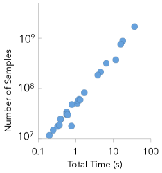
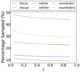
Figure 3: (a)Impact of data size (b) Scatter plot of samples vs runtime (c) Impact of $\delta$

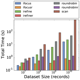
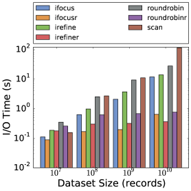
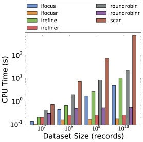
Figure 4: (a)Total time vs dataset size (b) I/O time vs dataset size (c) CPU time vs dataset size

5 Experiments

In this section, we experimentally evaluate our algorithms versus traditional sampling techniques on a variety of synthetic and real-world datasets. We evaluate the algorithms on three different metrics: the number of samples required (sample complexity), the accuracy of the produced results, and the wall-clock runtime performance on our prototype sampling system, NeedleTail.

5.1 Experimental Setup

Algorithms: Each of the algorithms we evaluate takes as a parameter $\delta$, a bound on the probability that the algorithm returns results that do not obey the ordering property. That is, all the algorithms are guaranteed to return results ordered correctly with probability $1-\delta$, no matter what the data distribution is.

The algorithms are as follows:

• IFocus ($\delta$): In each round, this algorithm takes an additional sample from all active groups, ensuring that the eventual output has accuracy greater than $1-\delta$, as described in Section 3.1. This algorithm is our solution for Problem 1.

• IFocusR ($\delta,r$): In each round, this algorithm takes an additional sample from all active groups, ensuring that the eventual output has accuracy greater than $1-\delta$, for a relaxed condition of accuracy based on resolution. Thus, this algorithm is the same as the previous, except that we stop at the granularity of the resolution value. This algorithm is our solution for Problem 2.

• IRefine ($\delta$): In each round, this algorithm divides all confidence intervals by half for all active groups, ensuring that the eventual output has accuracy greater than $1-\delta$, as described in Section 3.6. Since the algorithm is aggressive in taking samples to divide the confidence interval by half each time, we expect it to do worse than IFocus.

• IRefineR ($\delta,r$): This is the IRefine algorithm except we relax accuracy based on resolution as we did in IFocusR.

We compare our algorithms against the following baseline:

• RoundRobin ($\delta$): In each round, this algorithm takes an additional sample from all groups, ensuring that the eventual output respects the order with probability than $1-\delta$. This algorithm is similar to conventional stratified sampling schemes [8], except that the algorithm has the guarantee that the ordering property is met with probability greater than $1-\delta$. We adapted this from existing techniques to ensure that the ordering property is met with probability greater than $1-\delta$. We cannot leverage any pre-existing techniques since they do not provide the desired guarantee.

• RoundRobinR ($\delta,r$): This is the RoundRobin algorithm except we relax accuracy based on resolution as we did in IFocusR.

System: We evaluate the runtime performance of all our algorithms on our early-stage NeedleTail prototype. We measure both the CPU times and the I/O times in our experiments to definitively show that our improvements are fundamentally due to the algorithms rather than skilled engineering. In addition to our algorithms, we implement a Scan operation in NeedleTail, which performs a sequential scan of the dataset to find the true means for the groups in the visualization. The Scan operation represents an approach that a more traditional system, such as PostgreSQL, would take to solve the visualization problem. Since we have both our sampling algorithms and Scan implemented in NeedleTail, we may directly compare these two approaches. We ran all experiments on a 64-core Intel Xeon E7-4830 server running Ubuntu 12.04 LTS; however, all our experiments were single-threaded. We use 1MB blocks to read from disk, and all I/O is done using Direct I/O to avoid any speedups we would get from the file buffer cache. Finally, we would like to state that our NeedleTail prototype is still in its early stages. The current implementation runs on top of a basic bitmap/hash map implementation with little-to-no optimization code. We believe custom writing our own bitmap/hash map implementations could lead to substantial improvements in the CPU overhead. Parallelization is another way to get significant gains in performance. We can easily parallelize our sampling workload to fully utilize the I/O bandwidth since random sampling tends to be an independent operation. In short, with a few optimizations, we fully expect runtime performance of our algorithms to be even better than the results we present in the following sections.

Key Takeaways: Here are our key results from experiments in Sections 5.2 and 5.3:

(1) Our IFocus and IFocusR ($r$=1%) algorithms yield

• up to 80% and 98% reduction in sampling and 79% and 92% in runtime (respectively) as compared to RoundRobin, on average, across a range of very large synthetic datasets, and

• up to 70% and 85% reduction in runtime (respectively) as compared to RoundRobin, for multiple attributes in a realistic, large flight records dataset [20].

(2) The results of our algorithms (in all of the experiments we have conducted) always respect the correct ordering property.

5.2 Synthetic Experiments

We begin by considering experiments on synthetic data. The datasets we ran our experiments on are as follows:

• Truncated Normals (truncnorm): For each group, we select a mean $\sigma$ sampled uniformly at random from $[0,100]$, and select a variance $\Delta$ from $\{4,25,64,100\}$. We generate values from a normal distribution for each group using the selected values. These normals are truncated at 0 and 100 to ensure that the values are bounded.

• Mixture of Truncated Normals (mixture): For each group, we select a collection of normal distributions, in the following way: we select a number sampled at random from $\{1,2,3,4,5\}$, indicating the number of truncated normal distributions that comprise each group. For each of these truncated normal distributions, we select a mean $\sigma$ sampled at random from $[0,100]$, and a variance $\Delta$ sampled at random from $[1,10]$. We repeat this for each group.

• Bernoulli (bernoulli): For each group, we select a mean sampled at random from $[0,100]$. Then, we construct our group by sampling between two values $\{0,100\}$ with the bias equal to the chosen mean. Thus, this is a Bernoulli distribution [50] with a mean selected up front. Note that this distribution has higher variance than those that are normal.

• Hard Bernoulli (hard): Given a parameter $\gamma<2$, we fix the mean for group $i$ to be $40+\gamma\times i$, and then construct each group by sampling between two values $\{0,100\}$ with bias equal to the mean. Note that in this case, $\eta$, the smallest distance between two means, is equal to $\gamma$. Recall that $c^{2}/\eta^{2}$ is a proxy for how difficult the input instance is (and therefore, how many samples need to be taken). We study this scenario so that we can control the difficulty of the input instance.

Our default setup consists of $k=10$ groups, with $10M$ records in total, equally distributed across all the groups, with $\delta=0.05$ (the failure probability) and $r=1$. Each data-point is generated by repeating the experiment 100 times. That is, we construct 100 different datasets with each parameter value, and measure the number of samples taken when the algorithms terminate, whether the output respects the correct ordering property, and the CPU and I/O times taken by the algorithms. For the algorithms ending in R, i.e., those designed for a more relaxed property leveraging resolution, we check if the output respects the relaxed property rather than the more stringent property. We focus on the mixture distribution for most of the experimental results, since we expect it to be the most representative of real world situations, using the hard Bernoulli in a few cases. We have conducted extensive experiments with other distributions as well, and the results are similar. We will describe these experiments whenever the behavior for those distributions is significantly different.

Variation of Sampling and Runtime with Data Size: We begin by measuring the sample complexity and wall-clock times of our algorithms as the data set size varies.

Summary: Across a variety of dataset sizes, our algorithm IFocusR (respectively IFocus) performs better on sample complexity and runtime than IRefineR (resp. IRefine) which performs significantly better than RoundRobinR (resp. RoundRobin). Further, the resolution improvement versions take many fewer samples than the ones without the improvement. In fact, for any dataset size greater than $10^{8}$, the resolution improvement versions take a constant number of samples and still produce correct visualizations.

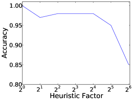
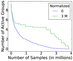
Figure 5: (a) Impact of heuristic shrinking factor on accuracy (b) Impact of heuristic shrinking factor for a harder case (c) Studying the number of active intervals as computation proceeds

Figure 3 shows the percentage of the dataset sampled on average as a function of dataset size (i.e., total number of tuples in the dataset across all groups) for the six algorithms above. The data size ranges from $10^{7}$ records to $10^{10}$ records (hundreds of GB). Note that the figure is in log scale.

Consider the case when dataset size = $10^{7}$ in Figure 3. Here RoundRobin samples $\approx$50% of the data, while RoundRobinR samples around 35% of the dataset. On the other hand, our IRefine and IRefineR algorithms both sample around 25% of the dataset, while IFocus samples around 15% and IFocusR around 10% of the dataset. Thus, compared to the vanilla RoundRobin scheme, all our algorithms reduce the number of samples required to reach the order guarantee, by up to $3\times$. This is because our algorithms focus on the groups that are actually contentious, rather than sampling from all groups uniformly.

As we increase the dataset size, we see that the sample percentage decreases almost linearly for our algorithms, suggesting that there is some fundamental upper bound to the number of samples required, confirming Theorem 3.5. With resolution improvement, this upper bound becomes even more apparent. In fact, we find that the raw number of records sampled for IFocusR, IRefineR, and RoundRobinR all remained constant for dataset sizes greater or equal to $10^{8}$. In addition, as expected, IFocusR (and IFocus) continue to outperform all other algorithms at all dataset sizes.

The wall-clock total, I/O, and CPU times for our algorithms running on NeedleTail can be found in Figures 4, 4, and 4, respectively, also in log scale. Figure 4 shows that for a dataset of size of $10^{9}$ records (8GB), IFocus/IFocusR take 3.9/0.37 seconds to complete, IRefine/IRefineR take 6.5/0.58 seconds to complete, RoundRobin/RoundRobinR take 18/1.2 seconds to complete, and Scan takes 89 seconds to complete. This means that IFocus/IFocusR has a 23$\times$ speedup and 241$\times$ speedup relative to Scan in producing accurate visualizations.

As the dataset size grows, the runtimes for the sampling algorithms also grow, but sublinearly, in accordance to the sample complexities. In fact, as alluded earlier, we see that the run times for IFocusR, IRefineR, and RoundRobinR are nearly constant for all dataset sizes greater than $10^{8}$ records. There is some variation, e.g., in I/O times for IFocusR at $10^{10}$ records, which we believe is due to random noise. In contrast, Scan yields linear scaling, leading to unusably long wall-clock (i.e., 898 seconds at $10^{10}$ records.)

We note that not only does IFocus beat out RoundRobin, and RoundRobin beat out Scan for every dataset size in total time, but this remains true for both I/O and CPU time as well. Sample complexities explain why IFocus should beat RoundRobin. It is more surprising that IFocus, which uses random I/O, outperforms Scan, which only uses sequential I/O. The answer is that so few samples are required the cost of additional random I/O is exceeded by the additional scan time; this becomes more true as the dataset size increases. As for CPU time, it highly correlated with the number of samples, so algorithms that operate on a smaller number of records outperform algorithms that need more samples.

The reason that CPU time for Scan is actually greater than the I/O time is that for every record read, it must update the mean and the count in a hash map keyed on the group. While Boost’s ${\tt unordered\_map}$ implementation is very efficient, our disk subsystem is able to read about 800 MB/sec, and a single thread on our machine can only perform about 10 M hash probes and updates / sec. However, even if we discount the CPU overhead of Scan, we find that total wall-clock time for IFocus and IFocusR is at least an order of magnitude better than just the I/O time for Scan. For $10^{10}$ records, compared to Scan’s 114 seconds of sequential I/O time, IFocus has a total runtime of 13 seconds, and IFocusR has a total runtime in 0.78 seconds, giving a speedup of at least 146$\times$ for a minimal resolution of 1%.

Finally, we relate the runtimes of our algorithms to the sample complexities with the scatter plot presented in Figure 3. The points on this plot represent the number of samples versus the total execution times of our sampling algorithms (excluding Scan) for varying dataset sizes. As is evident, the runtime is directly proportional to the number of samples. With this in mind, for the rest of the synthetic datasets, we focus on sample complexity because we believe it provides a more insightful view into the behavior of our algorithms as parameters are varied. We return to runtime performance when we consider real datasets in Section 5.3.

Variation of Sampling and Accuracy with $\delta$: We now measure how $\delta$ (the user-specified probability of error) affects the number of samples and accuracy.

Summary: For all algorithms, the percentage sampled decreases as $\delta$ increases, but not by much. The accuracy, on the other hand, stays constant at 100%, independent of $\delta$. Sampling any less to estimate the same confidence intervals leads to significant errors, indicating that the confidence intervals cannot shrink by much.

Figure 3 shows the effect of varying $\delta$ on the sample complexity for the six algorithms. As can be seen in the figure, the percentage of data sampled reduces but does not go to $0$ as $\delta$ increases. This is because the amount of sampling (as in Equation 4) is the sum of three quantities, one that depends on $\log k$, the other on $\log\delta$, and another on $\log\log(1/\eta_{i})$. The first and last quantities are independent of $\delta$, and thus the number of samples required is non-zero even as $\delta$ gets close to $1$. The fact that sampling is non-zero when $\delta$ is large is somewhat disconcerting; to explore whether this level of sampling is necessary, and whether we are being too conservative, we examine the impact of sampling less on accuracy (i.e., whether the algorithm obeys the desired visual property).

We focus on IFocusR  (similar results are observed for all algorithms, and other distributions) and consider the impact of shrinking confidence intervals at a rate faster than prescribed by IFocus in Line 6 of Algorithm 1. We call this rate the heuristic factor: a heuristic factor of 4 means that we divide the confidence interval as estimated by Line 6 by 4, thereby ensuring that the confidence interval overlaps are fewer in number, allowing the algorithms to terminate faster. We plot the average accuracy (i.e., the fraction of times the algorithm violates the visual ordering property) as a function of the heuristic factor in Figure 5 for $\delta=0.05$ (other $\delta$s give identical figures, as we will see below).

First, consider heuristic factor 1, which directly corresponds to IFocusR. As can be seen in the figure, IFocusR has 100% accuracy: the reason is that IFocusR ends up sampling a constant amount to ensure that the confidence intervals do not overlap, independent of $\delta$, enabling it to have perfect accuracy for this $\delta$. In fact, we find that all our 6 algorithms have accuracy 100%, independent of $\delta$ and the data distributions; thus, our algorithms not only provide much lower sample complexity, but also respect the visual ordering property on all datasets.

Next, we see that as we increase the heuristic factor, the accuracy immediately decreases (roughly monotonically) below 100%, Surprisingly, even with a heuristic factor of $2$, we start making mistakes at a rate greater than $2-3\%$ independent of $\delta$. Thus, even though our sampling is conservative, we cannot do much better, and are likely to make errors by shrinking confidence intervals faster than prescribed by Algorithm 1. To study this further, we plotted the same graph for the hard case with $\gamma=0.1$ (recall that $\gamma=\eta$ for this case), in Figure 5. Here, once again, for heuristic factor 1, i.e., IFocusR, the accuracy is 100%. On the other hand, even with a heuristic factor of 1.01, where we sample just 1% less to estimate the same confidence interval, the accuracy is already less than 95%. With a heuristic factor of 1.2, the accuracy is less than 70%! This result indicates that we cannot shrink our confidence intervals any faster than IFocusR does, since we may end up making up making far more mistakes than is desirable—even sampling just $1\%$ less can lead to critical errors.

Overall, the results in Figures 5 and 5 are in line with our theoretical lower bound for sampling complexity, which holds no matter what the underlying data distribution is. Furthermore, we find that algorithms backed by theoretical guarantees are necessary to ensure correctness across all data distributions (and heuristics may fail at a rate higher than $\delta$).

Rate of Convergence: In this experiment, we measure the rate of convergence of the IFocus algorithms in terms of the number of groups that still need to be sampled as the algorithms run.

Summary: Our algorithms converge very quickly to a handful of active groups. Even when there are still active groups, the number of incorrectly ordered groups is very small — thus, our algorithms can be used to provide incrementally improving partial results.

Figure 5 shows the average number of active groups as a function of the amount of sampling performed for IFocus, over a set of 100 datasets of size 10M. It shows two scenarios: $0$, when the number of samples is averaged across all 100 datasets and $3M$, when we average across all datasets where at least three million samples were taken. For $0$, on average, the number of active groups after the first 1M samples (i.e., 10% of the 10M dataset), is just 2 out of 10, and then this number goes down slowly after that. The reason for this is that, with high probability, there will be two groups whose $\mu_{i}$ values are very close to each other. So, to verify if one is greater than the other, we need to do more sampling for those two groups, as compared to other groups whose $\eta_{i}$ (the distance to the closest mean) is large—those groups are not active beyond 1M samples. For the $3M$ plot, we find that the number of samples necessary to reach 2 active groups is larger, close to 3.5M for the 3M case.

Next, we investigate if the current estimates $\nu_{i},\ldots,\nu_{k}$ respect the correct ordering property, even though some groups are still active. To study this, we depict the number of incorrectly ordered pairs as a function of the number of samples taken, once again for the two scenarios described above. As can be seen in Figure 6, even though the number of active groups is close to two or four at 1M samples, the number of incorrect pairs is very close to 0, but often has small jumps — indicating that the algorithm is correct in being conservative and estimating that the we haven’t yet identified the actual ordering. In fact, the number of incorrect pairs is non-zero up to as many as 3M samples, indicating that we cannot be sure about the correct ordering without taking that many samples. At the same time, since the number of incorrect pairs is small, if we are fine with displaying somewhat incorrect results, we can show the current results to to the user.

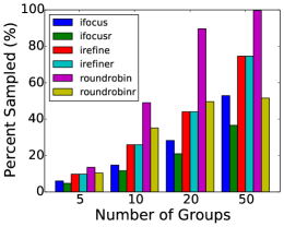
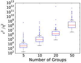
Figure 6: (a) Studying the number of incorrectly ordered pairs as computation proceeds (b) Impact of number of groups on sampling (c) Evaluating the difficulty as a function of number of groups

Variation of Sampling with Number of Groups: We now look at how the sample complexity varies with the number of groups.

Summary: As the number of groups increases, the amount of sampling increases for all algorithms as an artifact of our data generation process, however, our algorithms continue to perform significantly better than other algorithms.

To study the impact of the number of groups on sample complexity, we generate 100 synthetic datasets of type mixture where the number of groups varies from 5 to 50, and plot the percentage of the dataset sampled as a function of the dataset size. Each group has 1M items. We plot the results in Figure 6. As can be seen in the figure, our algorithms continue to give significant gains even when the number of groups increases from 5 to 50. However, we notice that the amount of sampling increases for IFocusR as the number of groups is increased, from less than 10% for 5 groups to close to 40% for 50 groups.

The higher sample complexity can be attributed to the dataset generation process. As a proxy for the “difficulty” of a dataset, Figure 6 shows the average $c^{2}/\eta^{2}$ as a function of the number of groups (recall that $\eta$ is the minimum distance between two means, $c$ is the range of all possible values, and that the sample complexity depends on $c^{2}/\eta^{2}$) The figure is a a box-and-whiskers plot with the y-axis on a log scale. Note that the average difficulty increases from $10^{4}$ for 5 to $10^{8}$ for 50–a 4 orders of magnitude increase! Since we are generating means for each group at random, it is not surprising that the more groups, the higher the likelihood that two randomly generated means will be close to each other.

Variation of Sampling with Proportion of Dataset: We now study the impact of skew on the algorithms.

Summary: Our algorithms continue to provide significant gains in the presence of skew in the underlying dataset.

We generated a variation of our 1M mixture dataset, where we vary the fraction of the dataset that belongs to the first group from 10% to 90%, while the remaining fraction is equally distributed among the remaining 9 groups. The results are depicted in Figure 7, where we once again show the amount of sampling as a function of the proportion of the dataset that the first group occupies. As can be seen in the figure, the relative gains of our IFocus and IFocusR  algorithms continue to hold even when the proportion is 90% (a highly skewed case). Note also that the amount of sampling goes down as the proportion increases: this is an artifact of our dataset generation mechanism. Since the dataset is generated randomly, the odds that the first group is part of the set of active intervals stays fixed, while if the first group was indeed among the active groups after 1M samples were taken, then we may need a lot more samples when the first group has a larger number of tuples, as compared to the other groups. Thus, the amount of total sampling goes down as the amount of skew increases.

Variation of Sampling with Standard Deviation: We now examine how the variance of the data affects the number of samples.

Summary: For truncnorm, as the standard deviation increases, the amount of sampling increases slightly.

To study the impact of the standard deviation of the groups in the dataset on the sampling performed, we focus on the truncnorm distribution, wherein each group is generated from a truncated normal distribution with a fixed standard deviation. We plot the average percentage of the dataset sampled by IFocusR  as a function of the $\delta$ (desired accuracy), for various values of the standard deviation of the groups in the dataset. The results are depicted in Figure 7. As can be seen in the figure, the percentage sampled is higher for larger standard deviations, but not by much (less than a 1-2% change across a range of standard deviations and $\delta$s).

To understand why the amount sampled for higher standard deviations is higher, we plot the average $c^{2}/\eta^{2}$ as a function of the standard deviation as a box-and-whiskers plot with the y-axis on a log scale in Figure 7. As can be seen in the figure, once again we find that the datasets generated with a higher standard deviation indeed have a higher “difficulty” (i.e., $c^{2}/\eta^{2}$), and so therefore, require more samples.

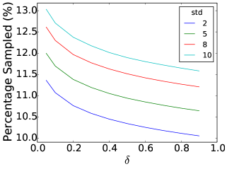
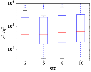
Figure 7: (a) Impact of the proportion of the first group on sampling (b) Impact of standard deviation on sampling for truncnorm (c) Evaluating the difficulty on varying standard deviation for truncnorm

5.3 Real Dataset Experiments

We next study the impact of our techniques on a real dataset.

Summary: IFocus and IFocusR take 50% fewer samples than RoundRobin irrespective of the attribute visualized.

For our experiments on real data, we used a flight records data set [20]. The data set contains the details of all flights within the USA from 1987–2008, with nearly 120 million records, taking up 12 GB uncompressed. From this flight data, we generated datasets of sizes 120 million records (2.4GB) and scaled-up 1.2 billion (24GB) and 12 billion records (240GB) for our experiments using probability density estimation. We focused on comparing our best algorithms—IFocus and IFocusR ($r$=1%)—versus the conventional sampling—RoundRobin. We evaluate the runtime performance for visualizing the averages for three attributes: Elapsed Time, Arrival Delay, and Departure Delay, grouped by Airline. For all algorithms and attributes, the orderings returned were correct.

The results are presented in Table 3. The first four rows correspond to the attribute Elapsed Time. Here, RoundRobin takes 32.6 seconds to return a visualization, whereas IFocus takes only 9.70 seconds (3$\times$ speedup) and IFocusR takes only 5.04 seconds (6$\times$ speedup). We see similar speedups for Arrival Delay and Departure Delay as well. As we move from the $10^{8}$ dataset to $10^{10}$ dataset, we see the run times roughly double for a 100$\times$ scale-up in the dataset. The reason for any increase at all in the runtime comes from the highly conflicting groups with means very close to one another. Our sampling algorithms may read all records in the group for these groups with with $\eta_{i}$ values. When the dataset size is increased to allow for more records to sample from, our sampling algorithms take advantage of this and sample more from the conflicting groups, leading to larger run times.

Attribute	Algorithm	$10^{8}$ (s)	$10^{9}$ (s)	$10^{10}$ (s)
Elapsed Time	RoundRobin	32.6	56.5	58.6
	IFocus	9.70	10.8	23.5
	IFocusR (1%)	5.04	6.64	8.46
Arrival Delay	RoundRobin	47.1	74.1	77.5
	IFocus	29.2	48.7	67.5
	IFocusR (1%)	9.81	15.3	16.1
Departure Delay	RoundRobin	41.1	72.7	76.6
	IFocus	14.3	27.5	44.3
	IFocusR (1%)	9.19	15.7	16.0

Table 3: Real Data Experiments

Regardless, we show that even on a real dataset, our sampling algorithms are able to achieve up to a 6$\times$ speedup in runtime compared to round-robin. We could achieve even higher speedups if we were willing to tolerate a higher minimum resolution.

6 Extensions

In this section, we describe a number of variations of our algorithm to handle different scenarios: either stronger or weaker conditions, or other types of queries or settings.

6.1 Weaker Conditions

We now describe extensions to IFocus to handle visual properties that are “weaker”, i.e., require much less samples.

6.1.1 Trends and Chloropleths

When viewing trend lines instead of bar graphs—where the $x$ axis is an ordinal attribute such as time—we instead want comparisons between consecutive pairs of groups to be accurate rather than all pairs. We state the problem below:

Problem 6.1 (AVG-Order-Trends).

Given a query $Q$, and values $c,\delta$, and an index on $X$, design a query processing algorithm returning estimates $\nu_{1},\ldots,\nu_{k}$ for $\mu_{1},\ldots,\mu_{k}$ which is as efficient as possible in terms of sample complexity ${\cal C}$, such that with probability greater than $1-\delta$, the ordering of $\nu_{1},\ldots,\nu_{k}$ with respect to $\mu_{1},\ldots,\mu_{k}$ is correct, where correctness is now defined as the following:

for all $i\in 1\ldots(k-1)$, if $\mu_{i}<\mu_{i+1}$ then $\nu_{i}<\nu_{i+1}$ if $\mu_{i}<\mu_{i+1}$ and vice versa.

Solution: The IFocus algorithm generalizes easily to the scenario where we only care about comparisons between neighboring groups instead of between all groups. In this case, we get the same sample complexity as now except that we replace the definition of $\eta_{i}$ to be $\eta_{i}^{*}=\min\{\tau_{i-1,i},\tau_{i,i+1}\}$, and our definition of active now changes to all groups whose confidence intervals overlap with confidence intervals of neighboring groups (rather than all groups).

Similarly, if, instead of a trend-line, we wished to generate a chloropleth (i.e., heat map) where adjacent regions are correctly ordered with respect to each other (or, even if we wanted to ensure that the regions that are close by are correctly ordered with respect to each other), then we can simply redefine active to mean all groups (here regions) whose confidence intervals overlap with confidence intervals of groups that are close by.

6.1.2 Top-$t$ Results

In many cases, the analyst is specifically interested in examining the top-$t$ or bottom-$t$ groups rather than all the groups. This is especially important if the number of groups is so large that the analyst cannot easily look at them all at once. In such a scenario, we need to make sure that we are confident about the fact that the $t$ groups we display are indeed the top or bottom $t$, and that these $t$ groups are ordered correctly with respect to each other.

Problem 6.2 (AVG-Order-Top-$t$).

Given a query $Q$, and values $c,\delta,t$, a minimum resolution $r$, and an index on $X$, design a query processing algorithm returning estimates $\nu^{\prime}_{1},\ldots,\nu^{\prime}_{t}$ for the largest $\mu^{\prime}_{1},\ldots,\mu^{\prime}_{t}$ which is as efficient as possible in terms of sample complexity ${\cal C}$, such that with probability greater than $1-\delta$, the ordering of $\nu_{1}^{\prime},\ldots,\nu_{t}^{\prime}$ with respect to $\mu_{t}^{\prime},\ldots,\mu_{t}^{\prime}$ is correct.

Solution: For this variant, our definition of active is now the groups for which either the confidence intervals overlap other confidence intervals AND we are not yet sure if they are part of the top-$t$ or not. As soon as we are sure that a group is not part of the top-$t$, based on their confidence interval, we remove them from the set of active groups. This approach once again guarantees correctness with probability greater than $1-\delta$.

6.1.3 Allowing Mistakes

In order to generate our visualizations quickly, consider the scenario when we are fine with making errors on $\gamma$% of the comparisons (in addition to $\delta$ probability error overall) Thus, we may be able to eliminate wasting effort on the most tricky comparisons, and focus instead on the easy ones. The problem is now:

Problem 6.3 (AVG-Order-Mistakes).

Given a query $Q$, and values $c,\delta,\gamma$, and an index on $X$, design a query processing algorithm returning estimates $\nu_{1},\ldots,\nu_{k}$ for $\mu_{1},\ldots,\mu_{k}$ which is as efficient as possible in terms of sample complexity ${\cal C}$, such that with probability greater than $1-\delta$, the ordering of $\nu_{1},\ldots,\nu_{k}$ with respect to $\mu_{1},\ldots,\mu_{k}$ is correct, where correctness is now defined as the following:

for $\gamma$ fraction or more of the pairs $(i,j),i\neq j$, the following holds: if $\mu_{i}<\mu_{j}$ then $\nu_{i}<\nu_{j}$ and vice versa.

Solution: The algorithm for this problem is easy to state as a modification of IFocus: we simply keep track of the fraction of correct pairs that we correctly know the ordering of (these are simply pairs of all inactive groups). Once the desired fraction $\gamma$ is met, the algorithm terminates and the estimates are returned.

6.2 Stronger Conditions

We now describe extensions to IFocus that are “stronger”, i.e., require more samples than IFocus.

6.2.1 Approximate Actual Values

We now consider the generalization where in addition to providing a ordering guarantee, we would like to ensure that the estimated averages per group is close to the actual averages. The problem, therefore, is:

Problem 6.4 (AVG-Order-Actual).

Given a query $Q$, and values $c,\delta$, a minimum approximation value $d$, and an index on $X$, design a query processing algorithm returning estimates $\nu_{1},\ldots,\nu_{k}$ for $\mu_{1},\ldots,\mu_{k}$ which is as efficient as possible in terms of sample complexity ${\cal C}$, such that with probability greater than $1-\delta$, the ordering of $\nu_{1},\ldots,\nu_{k}$ with respect to $\mu_{1},\ldots,\mu_{k}$ is correct, and for all $i\in 1\ldots k,|\nu_{i}-\mu_{i}|\leq d$.

Solution: For this variant, we first ensure a minimum amount of sampling $m$ such that $\varepsilon\geq d/2$. Once we perform the minimum amount of sampling, the IFocus algorithm proceeds as before. The sample complexity for this algorithm is the same as that for IFocus (as listed in Theorem 3.5) except that $\eta_{i}$ is replaced with $\min\{\eta_{i},d/2\}$.

6.2.2 Partial Results

Our IFocus algorithm is provably optimal in that it lets us get to the correct ordering with the least amount of samples. In many cases, it would be useful to show the analyst the estimated averages of the groups whose values we are already confident about, so that they can start viewing and analyzing “partial” results.

Problem 6.5 (AVG-Order-Partial).

Given a query $Q$, and values $c,\delta$, a minimum resolution $r$, and an index on $X$, design a query processing algorithm returning estimates $\nu_{1},\ldots,\nu_{k}$ for $\mu_{1},\ldots,\mu_{k}$ which is as efficient as possible in terms of sample complexity ${\cal C}$, such that with probability greater than $1-\delta$, the ordering of $\nu_{1},\ldots,\nu_{k}$ with respect to $\mu_{1},\ldots,\mu_{k}$ is correct; and the algorithm outputs each estimate $\nu_{i}$ as soon as it is sure about it.

Solution: Our solution for this variant is straightforward: we simply output the estimates for each group as soon as they become inactive. We have the following guarantee: with probability $1-\delta$, the ordering between all groups whose estimates are output at any stage in the algorithm is correct. Further, the sample complexity to get to the first $k^{\prime}$ groups being output is the following:

$$O\left(\frac{c^{2}k^{\prime}}{\eta_{k^{\prime}}^{\prime}}(\log(\frac{k}{\delta})+\log\log(\frac{1}{\eta_{k^{\prime}}^{\prime}}))\right)$$

where $\eta_{k^{\prime}}^{\prime}$ is the smallest $\eta_{i}$ among the first $k^{\prime}$ groups to become inactive.

6.3 Other Settings and Queries

Our techniques can be adapted to a number of other settings or more complex queries.

6.3.1 Different Aggregation Functions: SUM

So far, we have focused our attention on estimating the ${\tt AVG}$ value of each group, ensuring that the correct ordering property is maintained. We now discuss extending our algorithms to estimate ${\tt SUM}$ instead of average.

Known Group Sizes: If we know the number of elements in each group, the two problems are equivalent; the sum $\sigma_{i}$ of the elements in the group $S_{i}$ is related to the average $\mu_{i}$ value of the elements in the group via the basic identity $\sigma_{i}=\mu_{i}\cdot|S_{i}|$. However, the algorithm needs to change slightly in order to correctly compute confidence intervals in this setting. Specifically, in Statement 6 and 9, we multiply the right hand side with $|S_{i}|$; and our estimates $\nu_{i}$ now correspond to estimates of $\sigma_{i}$ instead of $\mu_{i}$.

The algorithm is listed in Algorithm 4.

Data: $S_{1},\ldots,S_{k},\delta$

1 Initialize $m\leftarrow 1$;

2 Draw $m$ samples from each of $S_{1},\ldots,S_{k}$ to provide initial estimates $\nu_{1},\ldots,\nu_{k}$;

3 Initialize $A=\{1,\ldots,k\}$;

4 while $A\neq\emptyset$ do

5       $m\leftarrow m+1$;

6       for each $i\in A$ do

7             $\varepsilon_{i}=c\,|S_{i}|\,\sqrt{\frac{2\log\log(m)+\log(\pi^{2}k/3\delta)}{2m}}$;

8            

9      for each $i\in A$ do

10             Draw a sample $x$ from $S_{i}$;

11             $\nu_{i}\leftarrow|S_{i}|(\frac{m-1}{m}\nu_{i}+\frac{1}{m}x$);

12            

13      for each $i\in A$ do

14             if $[\nu_{i}-\varepsilon_{i},\nu_{i}+\varepsilon_{i}]\cap\big{(}\bigcup_{j\in A\setminus\{i\}}[\nu_{j}-\varepsilon_{j},\nu_{j}+\varepsilon_{j}]\big{)}=\emptyset$ then

15                  $A\leftarrow A\setminus\{i\}$

16            

17      

18Return $\nu_{1},\ldots,\nu_{k}$;

Algorithm 4 IFocus–Sum1

Unknown Group Sizes: When we don’t know the number of tuples in each group, then our problem becomes a bit more complicated, since we need to simultaneously estimate both the sizes of the groups, as well as the average, in order to be able to estimate ${\tt SUM}$ overall across all groups. For the purposes of this discussion, we assume that we know the total number of elements in all the groups; however, our algorithm does not depend on this knowledge. If the total number of elements across all groups is known, we can start reasoning about fractional sizes. We let $s_{i}=\frac{|S_{i}|}{\sum_{j=1}^{k}|S_{j}|}$ to denote the fractional size of $S_{i}$. Then $\sigma_{i}=s_{i}\mu_{i}$ is the normalized sum of the elements in the set $S_{i}$. The problem of estimating the sums ensuring correct ordering is identical to that of estimating the normalized sums with correct ordering, so we now focus on the latter.

Using our NeedleTail indexes, when we retrieve an additional tuple from $S_{i}$, we can also estimate the number of tuples we needed to skip over until we reach the tuple that belongs to $S_{i}$. NeedleTail’s in-memory bitmap indexes allow us to retrieve this information without doing any disk seeks. This number allows us to get unbiased estimates for the normalized sums $s_{1}\mu_{1},\ldots,s_{k}\mu_{k}$. Then if $x$ is a random element from $S_{i}$ and $z$ is a random unbiased estimate of $s_{i}$, the random variable $x\cdot z$ is an unbiased estimate of $\sigma_{i}$. The random variable $x\cdot z$ is also in the range $[0,c]$, so we again can apply Hoeffding inequalities to derive and analyze an algorithm that is very similar to the original IFocus. The only difference between IFocus and this new algorithm is that we simultaneously get samples for $x$ and $z$; the confidence interval computation stays unchanged.

The fact that the confidence interval computation looks exactly the same as when we’re computing the average is somewhat surprising, since we’re trying to estimate the size of each group as well as the average—one may expect the confidence intervals to be larger than before. In the worst case, when all the groups have the same size (which is identical to when we’re estimating the average), this is essentially what happens. If the group $S_{i}$ has average value $\mu_{i}$, then its normalized sum is now $\mu_{i}/k$, i.e., the normalized sums are all $k$ times smaller than the corresponding averages. But since our confidence intervals shrink at the same pace in the average and normalized sum cases, it will take much longer to be small enough to avoid overlaps for normalized sums. Specifically, this will require a number of samples that is roughly $k^{2}$ times larger in the normalized sum case than in the average case. However, we do expect groups to be widely varying in size, in which case, we do not expect the additional $k^{2}$ factor to affect the sample complexity.

The pseudocode for the Algorithm can be found in Algorithm 5.

Data: $S_{1},\ldots,S_{k},\delta$

1 Initialize $m\leftarrow 1$;

2 Draw $m$ samples from each of $S_{1},\ldots,S_{k}$ to provide initial estimates $\nu_{1},\ldots,\nu_{k}$;

3 Initialize $A=\{1,\ldots,k\}$;

4 while $A\neq\emptyset$ do

5       $m\leftarrow m+1$;

6       $\varepsilon_{i}=c\,\sqrt{\frac{2\log\log(m)+\log(\pi^{2}k/3\delta)}{2m}}$;

7       for each $i\in A$ do

8             Draw a sample $x$ from $S_{i}$;

9             Draw an estimate $z$ of the size $s_{i}$;

10             $\nu_{i}\leftarrow\frac{m-1}{m}\nu_{i}+\frac{1}{m}xz$;

11            

12      for each $i\in A$ do

13             if $[\nu_{i}-\varepsilon_{i},\nu_{i}+\varepsilon_{i}]\cap\big{(}\bigcup_{j\in A\setminus\{i\}}[\nu_{j}-\varepsilon_{j},\nu_{j}+\varepsilon_{j}]\big{)}=\emptyset$ then

14                  $A\leftarrow A\setminus\{i\}$

15            

16      

17Return $\nu_{1},\ldots,\nu_{k}$;

Algorithm 5 IFocus–Sum2

6.3.2 Different Aggregation Functions: COUNT

Naturally, estimating ${\tt COUNT}$ per group is trivial if the number of tuples per group is known. If the number of tuples is not known (while the total number of tuples is known), we can simply apply the algorithm for ${\tt SUM}$, while only getting samples for $s_{i}$, rather than $\sigma_{i}$. Note that $s_{i}\in[0,1]$ rather than $[0,c]$ like in the previous case.

6.3.3 Selection Predicates

Consider the scenario when we have a query of the form:

${\tt SELECT}\ \ X,\ \ {\tt AVG}(Y)\ \ {\tt FROM}\ \ R(X,\ Y,\ldots)\ \ {\tt GROUP}\ \ {\tt BY}\ \ X\ \ {\tt WHERE}\ \$Pred

Here, we may have additional predicates on $X,Y$ or other attributes. For instance, we may want to view the average delay of all airlines whose delay is more than half an hour, i.e., the flights with a long delay.

Solution: Our algorithms still continue to work even if we have selection predicates on one more more attributes, as long as we have an index on the group-by attribute (the case where we do not have an index on the group-by attribute is captured in Section 6.3.6). Here, NeedleTail’s bitmap indexes allow us to retrieve, on demand, tuples that are from any specific group $S_{i}$, and also satisfy the selection conditions specified.

6.3.4 Multiple Group-bys

If $Q$ consists of multiple group bys, for instance:

${\tt SELECT}\ \ X,\ Z,\ \ {\tt AVG}(Y)\ \ {\tt FROM}\ \ R(X,\ Y,\ Z)\ \ {\tt GROUP}\ \ {\tt BY}\ \ X,\ Z$

Here, we may want to view a three-dimensional visualization or a two-dimensional visualization with the cross-product of the $X,Z$ values on the X axis. For instance, we may want to see the average delay of all flights by airline and origin airport.

Solution: In this case, we can simply apply the same algorithms as long as we have either a joint index on $X$ and $Z$, or an index on either $X$ or $Z$. When we have an index on just $X$ or just $Z$, the algorithms can still operate correctly, but may have a higher sample complexity. Say we have an index only on $X$. In such a case, we continue taking samples from the groups with $X=x_{i}$, as long as there is some value $z_{j}$, such that the group corresponding to $(x_{i},z_{j})$ is still active.

6.3.5 Multiple Aggregates Visualized

Consider the scenario when the analyst wishes to visualize multiple aggregates, as the following query indicates:

${\tt SELECT}\ \ X,\ {\tt AVG}(Z),\ {\tt AVG}(Y)\ \ {\tt FROM}\ \ R(X,\ Y,\ Z)\ \ {\tt GROUP}\ \ {\tt BY}\ \ X$

Problem 6.6 (AVG-AVG-Order).

Given a query $Q$, and values $c,\delta$, a minimum resolution $r$, and an index on $X$, design a query processing algorithm returning estimates $\nu_{11},\ldots,\nu_{1k}$ for $\mu_{11},\ldots,\mu_{1k}$ (true averages of $Y$), and $\nu_{21},$ $\ldots,$ $\nu_{2k}$ for $\mu_{21},$ $\ldots,$ $\mu_{2k}$ (true averages of $Z$), which is as efficient as possible in terms of sample complexity ${\cal C}$, such that with probability greater than $1-\delta$, the ordering of $\nu_{i1},\ldots,$ $\nu_{ik}$ with respect to $\mu_{i1},\ldots,\mu_{ik}$ is correct for both $i=1,2$.

Solution: In this case, we apply IFocus  to the problem of ${\tt AVG}(Y)$ first (with $\delta$ set as $\delta/2$), while also simultaneously estimating ${\tt AVG}(Z)$. Then, once there are no longer any more active groups, we apply IFocus to ${\tt AVG}(Z)$ (with $\delta$ set as $\delta/2$), starting at the estimates we already have. In the worst case, the sample complexity will be the sum of the sample complexities of running the two independently, but since the second iteration of IFocus will start having sampled quite a few values per group for ${\tt AVG}(Z)$, the samples taken for the second iteration of IFocus is likely to be much smaller than the first.

6.3.6 No Indexes

We now consider the scenario when there is no index on the group-by attribute $X$. The new problem in this scenario can be stated as the following:

Problem 6.7 (AVG-Order-NoIndex).

Given a query $Q$, and values $c,\delta$, design a query processing algorithm returning estimates $\nu_{1},\ldots,\nu_{k}$ for $\mu_{1},\ldots,\mu_{k}$ which is as efficient as possible in terms of sample complexity ${\cal C}$, such that with probability greater than $1-\delta$, the ordering of $\nu_{1},\ldots,\nu_{k}$ with respect to $\mu_{1},\ldots,\mu_{k}$ is correct.

We assume that no other indexes are present. Without an index on $X$, we cannot sample from specific groups; we can only get a random sample from any one of the groups. However, we can still use Hoeffding’s inequality to decide when to terminate taking random samples. If the number of tuples per group is roughly the same, the performance of this algorithm would be similar to the performance of a round robin approach that takes a sample from all groups no matter if they are active or not. This approach, although poor compared to IFocus, allows us to get away by sampling much less of the dataset (as we will see in Section 5).

7 Related Work

The work related to our paper can be placed in a few categories:

Approximate Query Processing: There are two categories of related work in approximate query processing: online, and offline. We focus on online first since it is more closely related to our work.

Online aggregation [28] is perhaps the most related online approximate query processing work. It uses conventional round-robin stratified sampling [8] (like RoundRobin) to construct confidence intervals for estimates of averages of groups. In addition, online aggregation provides an interactive tool that allows users to stop processing of certain groups when their confidence is “good enough”. Thus, the onus is on the user to decide when to stop processing groups (if not, stratified sampling is employed for all groups). Here, since our target is a visualization with correct properties, IFocus automatically decides when to stop processing groups. Hence, we remove the burden on the user, and prevent the user from stopping a group too early (making a mistake), or too late (doing extra work).

There are other papers that also use round-robin stratified sampling for various purposes, primarily for COUNT estimation respecting real-time constraints [31], respecting accuracy constraints (e.g., ensuring that confidence intervals shrink to a pre-specified size) without indexes [30], and with indexes [39, 26].

Since visual guarantees in the form of relative ordering is very different from the kind of objectives prior work in online approximate query processing considered, our techniques are quite different. Most papers on online sampling for query processing, including [30, 31, 39, 28], either use uniform random sampling or round-robin stratified sampling. Uniform random sampling is strictly worse than round-robin stratified sampling (e.g., if the dataset is skewed) and in the best case is going to be only as good, which is why we chose not to compare it in the paper. On the other hand, we demonstrate that conventional sampling schemes like round-robin stratified sampling sample a lot more than our techniques.

Next, we consider offline approximate query processing. Over the past decade, there has been a lot of work on this topic; as examples, see [22, 33, 9]. Garofalakis et al. [21] provides a good survey of the area; systems that support offline approximate query processing include BlinkDB[3] and Aqua [2]. Typically, offline schemes achieve a user-specified level of accuracy by running the query on a sample of a database. These samples are chosen a-priori, typically tailored to a workload or a small set of queries [1, 32, 5, 4, 10]. In our case, we do not assume the presence of a precomputed sample, since we are targeting ad-hoc visualizations. Even when precomputing samples, a common strategy is to use Neyman Allocation [12], like in [11, 34], by picking the number of samples per strata to be such that the variance of the estimate from each strata is the same. In our case, since we do not know the variance up front from each strata (or group), this defaults once again to round-robin stratified sampling. Thus, we believe that round-robin stratified sampling is an appropriate and competitive baseline, even here.

Statistical Tests: There are a number of statistical tests [50, 8] used to tell if two distributions are significantly different, or whether one hypothesis is better than a set of hypotheses (i.e., statistical hypothesis testing). Hypothesis testing allows us to determine, given the data collected so far, whether we can reject the null hypothesis. The $t$-test [8] specifically allows us to determine if two normal distributions are different from each other, while the Whitney-Mann-U-test [43] allows us to determine if two arbitrary distributions are different from each other, None of these tests can be directly applied to decide where to sample from a collection of sets to ensure that the visual ordering property is preserved.

Noisy Sorting: Our work is also related to sorting with noisy comparisons, both in the context of error-prone processing units [16], or human workers [25, 13]. In our case, we cannot directly ask for comparisons between two groups, we can only get additional samples per group, and these additional samples can help all the comparisons that the specific group is involved in.

Visualization Tools: Over the past few years, the visualization community has introduced a number of interactive visualization tools such as ShowMe, Polaris, Tableau, and Profiler [48, 35, 27]. Similar visualization tools have also been introduced by the database community, including Fusion Tables [23], VizDeck [36], and Devise [42]. A recent vision paper [44] has proposed a tool for recommending interesting visualizations of query results to users. All these tools could benefit from the algorithms outlined in this paper to improve performance while preserving visual properties.

Scalable Visualization: There has been some recent work on scalable visualizations from the information visualization community as well. Immens [41] and Profiler [35] maintain a data cube in memory and use it to support rapid user interactions. While this approach is possible when the dimensionality and cardinality is small (e.g., for simple map visualizations of a single attribute), it cannot be used when ad-hoc queries are posed. A related approach uses precomputed image tiles for geographic visualization [17].

Other recent work has addressed other aspects of visualization scalability, including prefetching and caching [14], data reduction [6] leveraging time series data mining [15], clustering and sorting [24, 45], and dimension reduction [54]. These techniques are orthogonal to our work, which focuses on speeding up the computation of a single visualization online.

Recent work from the visualization community has also demonstrated via user studies on simulations that users are satisfied with uncertain visualizations generated for algorithms like online aggregation, as long as the visualization shows error bars [18, 19]. This work supports our core premise, that analysts are willing to use inaccurate visualizations as long as the trends and comparisons of the output visualizations are accurate.

Learning to Rank: The goal of learning to rank [40] is the following: given training examples that are ranked pairs of entities (with their features), learn a function that correctly orders these entities. While the goal of ordering is similar, in our scenario we assume no relationships between the groups, nor the presence of features that would allow us to leverage learning to rank techniques.

8 Conclusions

Our experience speaking with data analysts is indeed that they prefer quick visualizations that look similar to visualizations that are computed on the entire database. Overall, increasing interactivity (by speeding up the processing of each visualization, even if it is approximate) can be a major productivity boost. As we demonstrated in this paper, we are able to generate visualizations with correct visual properties on querying less than 0.02% of the data on very large datasets (with $10^{10}$ tuples), giving us a speed-up of over 60$\times$ over other schemes (such as RoundRobin) that provide similar guarantees, and 1000$\times$ over the scheme that simply generates the visualization on the entire database.

References

- [1] S. Acharya, P. B. Gibbons, and V. Poosala. Congressional samples for approximate answering of group-by queries. SIGMOD, pages 487–498, 2000.
- [2] S. Acharya, P. B. Gibbons, V. Poosala, and S. Ramaswamy. The aqua approximate query answering system. SIGMOD, pages 574–576, 1999.
- [3] S. Agarwal et al. Blinkdb: queries with bounded errors and bounded response times on very large data. In EuroSys, pages 29–42, 2013.
- [4] N. Alon, Y. Matias, and M. Szegedy. The space complexity of approximating the frequency moments. In STOC, pages 20–29, 1996.
- [5] B. Babcock, S. Chaudhuri, and G. Das. Dynamic sample selection for approximate query processing. SIGMOD, pages 539–550, 2003.
- [6] G. Burtini et al. Time series compression for adaptive chart generation. In CCECE 2013, pages 1–6. IEEE, 2013.
- [7] R. Canetti, G. Even, and O. Goldreich. Lower bounds for sampling algorithms for estimating the average. Inf. Process. Lett., 53(1):17–25, 1995.
- [8] G. Casella and R. Berger. Statistical Inference. Duxbury, June 2001.
- [9] K. Chakrabarti, M. N. Garofalakis, R. Rastogi, and K. Shim. Approximate query processing using wavelets. In VLDB, pages 111–122, 2000.
- [10] S. Chaudhuri, G. Das, M. Datar, R. Motwani, and V. Narasayya. Overcoming limitations of sampling for aggregation queries. In ICDE, pages 534–542, 2001.
- [11] S. Chaudhuri, G. Das, and V. Narasayya. Optimized stratified sampling for approximate query processing. ACM Trans. Database Syst., 32(2), June 2007.
- [12] W. G. Cochran. Sampling techniques. John Wiley & Sons, 1977.
- [13] S. B. Davidson, S. Khanna, T. Milo, and S. Roy. Using the crowd for top-k and group-by queries. ICDT ’13, pages 225–236, 2013.
- [14] P. R. Doshi, E. A. Rundensteiner, and M. O. Ward. Prefetching for visual data exploration. In DASFAA 2003, pages 195–202. IEEE, 2003.
- [15] P. Esling and C. Agon. Time-series data mining. ACM Computing Surveys (CSUR), 45(1):12, 2012.
- [16] U. Feige, P. Raghavan, D. Peleg, and E. Upfal. Computing with noisy information. SIAM J. Comput., 23:1001–1018, October 1994.
- [17] D. Fisher. Hotmap: Looking at geographic attention. IEEE Computer Society, November 2007. Demo at http://hotmap.msresearch.us.
- [18] D. Fisher. Incremental, approximate database queries and uncertainty for exploratory visualization. In LDAV’11, pages 73–80, 2011.
- [19] D. Fisher, I. O. Popov, S. M. Drucker, and M. C. Schraefel. Trust me, I’m partially right: incremental visualization lets analysts explore large datasets faster. In CHI’12, pages 1673–1682, 2012.
- [20] Flight Records. http://stat-computing.org/dataexpo/2009/the-data.html. 2009.
- [21] M. N. Garofalakis and P. B. Gibbons. Approximate query processing: Taming the terabytes. VLDB, pages 725–, 2001.
- [22] P. B. Gibbons. Distinct sampling for highly-accurate answers to distinct values queries and event reports. In VLDB, pages 541–550, 2001.
- [23] H. Gonzalez et al. Google fusion tables: web-centered data management and collaboration. In SIGMOD Conference, pages 1061–1066, 2010.
- [24] D. Guo. Coordinating computational and visual approaches for interactive feature selection and multivariate clustering. Information Visualization, 2(4):232–246, 2003.
- [25] S. Guo, A. Parameswaran, and H. Garcia-Molina. So who won?: dynamic max discovery with the crowd. In SIGMOD Conference, pages 385–396, 2012.
- [26] P. J. Haas et al. Selectivity and cost estimation for joins based on random sampling. J. Comput. Syst. Sci., 52(3):550–569, 1996.
- [27] P. Hanrahan. Analytic database technologies for a new kind of user: the data enthusiast. In SIGMOD Conference, pages 577–578, 2012.
- [28] J. M. Hellerstein, P. J. Haas, and H. J. Wang. Online aggregation. In SIGMOD Conference, 1997.
- [29] W. Hoeffding. Probability inequalities for sums of bounded random variables. Journal of the American statistical association, 58(301):13–30, 1963.
- [30] W.-C. Hou, G. Özsoyoglu, and B. K. Taneja. Statistical estimators for relational algebra expressions. In PODS, pages 276–287, 1988.
- [31] W.-C. Hou, G. Özsoyoglu, and B. K. Taneja. Processing aggregate relational queries with hard time constraints. In SIGMOD Conference, pages 68–77, 1989.
- [32] Y. E. Ioannidis and V. Poosala. Histogram-based approximation of set-valued query-answers. VLDB ’99, pages 174–185, 1999.
- [33] C. Jermaine, S. Arumugam, A. Pol, and A. Dobra. Scalable approximate query processing with the dbo engine. ACM Trans. Database Syst., 33(4), 2008.
- [34] S. Joshi and C. Jermaine. Robust stratified sampling plans for low selectivity queries. In ICDE 2008, pages 199–208. IEEE, 2008.
- [35] S. Kandel et al. Profiler: integrated statistical analysis and visualization for data quality assessment. In AVI, pages 547–554, 2012.
- [36] A. Key, B. Howe, D. Perry, and C. Aragon. Vizdeck: Self-organizing dashboards for visual analytics. SIGMOD ’12, pages 681–684, 2012.
- [37] A. Kim, S. Madden, and A. Parameswaran. Needletail: A system for browsing queries (demo). In Technical Report, Available at: i.stanford.edu/~adityagp/ntail-demo.pdf, 2014.
- [38] N. Koudas. Space efficient bitmap indexing. In CIKM, pages 194–201, 2000.
- [39] R. J. Lipton et al. Efficient sampling strategies for relational database operations. Theor. Comput. Sci., 116(1&2):195–226, 1993.
- [40] T.-Y. Liu. Learning to rank for information retrieval. Foundations and Trends in Information Retrieval, 3(3):225–331, 2009.
- [41] Z. Liu, B. Jiang, and J. Heer. immens: Real-time visual querying of big data. Computer Graphics Forum (Proc. EuroVis), 32, 2013.
- [42] M. Livny et al. Devise: Integrated querying and visualization of large datasets. In SIGMOD Conference, pages 301–312, 1997.
- [43] H. B. Mann and D. R. Whitney. On a test of whether one of two random variables is stochastically larger than the other. The annals of mathematical statistics, pages 50–60, 1947.
- [44] A. Parameswaran, N. Polyzotis, and H. Garcia-Molina. SeeDB: Visualizing Database Queries Efficiently. In VLDB, 2014.
- [45] J. Seo et al. A rank-by-feature framework for interactive exploration of multidimensional data. Information Visualization, pages 96–113, 2005.
- [46] R. J. Serfling et al. Probability inequalities for the sum in sampling without replacement. The Annals of Statistics, 2(1):39–48, 1974.
- [47] Spotfire Inc. spotfire.com (retrieved March 24, 2014).
- [48] C. Stolte, D. Tang, and P. Hanrahan. Polaris: a system for query, analysis, and visualization of multidimensional databases. Commun. ACM, 51(11), 2008.
- [49] E. R. Tufte and P. Graves-Morris. The visual display of quantitative information, volume 2. Graphics press Cheshire, CT, 1983.
- [50] L. Wasserman. All of Statistics. Springer, 2003.
- [51] Wikipedia. Jensen’s inequality — wikipedia, the free encyclopedia, 2014. [Online; accessed 16-May-2014].
- [52] K. Wu et al. Analyses of multi-level and multi-component compressed bitmap indexes. ACM Trans. Database Syst., 35(1), 2010.
- [53] K. Wu, E. J. Otoo, and A. Shoshani. Optimizing bitmap indices with efficient compression. ACM Trans. Database Syst., 31(1):1–38, 2006.
- [54] J. Yang et al. Visual hierarchical dimension reduction for exploration of high dimensional datasets. VISSYM ’03, pages 19–28, 2003.