On spectral asymptotic of quasi-exactly solvable quartic potential

Abstract.

Motivated by the earlier results of [19] and [26], we discuss below the asymptotic of the solvable part of the spectrum for the quasi-exactly solvable quartic oscillator. In particular, we formulate a conjecture on the coincidence of the asymptotic shape of the level crossings of the latter oscillator with the asymptotic shape of zeros of the Yablonskii-Vorob’ev polynomials. Further we present a numerical study of the spectral monodromy for the oscillator in question.

1. Introduction

A quasi-exactly solvable quartic oscillator was introduced by C. M. Bender and S. Boettcher in [1] and (in its restricted form) is a Schrödinger-type eigenvalue problem of the form

$$L_{J}(w)=w^{\prime\prime}-(x^{4}/4-ax^{2}/2-Jx)w=\lambda w$$ (1.1)

with the boundary conditions $w(t)\to 0$ and $w(te^{2\pi i/3})\to 0$ as $t\to+\infty,$ where $a\in\mathbb{C}$ and $J$ are parameters of the spectral problem. With these boundary conditions, real $a$ and $J$, (1.1) is not a Hermitian but is a $PT$-symmetric operator, see [24], [19] and [13]. If $J=n+1$ is a positive integer, then $L_{n+1}(w)$ maps the linear space of quasi-exactly solutions of the form $\{pe^{-x^{3}/6+ax/2}:\deg p\leq n\}$ to itself where $p$ belongs to the linear space of univariate polynomials of degree at most $n$. The restriction of the operator $L_{n+1}(w)$ to the latter linear space is a finite-dimensional linear operator whose spectrum and eigenfunctions can be found explicitly using methods of linear algebra. This part of the spectrum and eigenfunctions of (1.1) is usually referred to as solvable. (Observe that the operator $L_{J}(w)$ given by (1.1) has a negative spectrum while physicists usually prefer to work with $-L_{J}(w)$ whose spectrum is positive.)

One can easily show that polynomial factors $p$ in the quasi-exactly solutions $w=pe^{h}$ of (1.1) coincide with the polynomial solutions of the degenerate Heun equation

$$y^{\prime\prime}-(x^{2}-a)y^{\prime}+(\alpha x-\lambda)y=0,$$ (1.2)

where $a\in\mathbb{C}$ has the same meaning as above and $(\alpha,\lambda)$ are the spectral variables. Obviously, if equation (1.2) has a polynomial solution of degree $n,$ then $\alpha=n$. Furthermore, to get a polynomial solution of (1.2) of degree $n$, the remaining spectral variable $\lambda$ should be chosen as an eigenvalue of the operator

$$T_{n}(y)=y^{\prime\prime}-(x^{2}-a)y^{\prime}+nxy$$ (1.3)

acting on the linear space of polynomials of degree at most $n.$

In the standard monomial basis $\{1,x,x^{2},\dots,x^{n}\}$ of the latter linear space, the action of the operator $T_{n}$ is given by the $4$-diagonal $(n+1)\times(n+1)$-matrix of the form

$$M_{n}^{(a)}:=\left(\begin{matrix}0&a&2&0&0&\cdots&0\\ n&0&2a&6&0&\cdots&0\\ 0&n-1&0&3a&12&\cdots&0\\ \vdots&\vdots&\ddots&\ddots&\ddots&\ddots&\vdots\\ 0&0&\cdots&3&0&(n-1)a&n(n-1)\\ 0&0&\cdots&0&2&0&na\\ 0&0&\cdots&0&0&1&0\end{matrix}\right).$$ (1.4)

We will call the bivariate characteristic polynomial $Sp_{n}(a,\lambda):=\det(M_{n}^{(a)}-\lambda I)$ the $n$-th spectral polynomial of (1.2). The degree of $Sp_{n}(a,\lambda)$ equals $n+1$ which is also its degree with respect to the variable $\lambda$. (The maximal degree of the variable $a$ in $Sp_{n}(a,\lambda)$ equals $\left[\frac{n+1}{2}\right]$). Additionally observe that for $a\in{\mathbb{R}}$, $Sp_{n}(a,\lambda)$ is a real polynomial in $\lambda$ and therefore the spectrum of $M_{n}^{(a)}$ is symmetric with respect to the real axis.

The main goal of this paper is to study the asymptotic of the spectrum of $M_{n}^{(a_{n})}$ in two different regimes. In the first regime we require that $\lim_{n\to\infty}\frac{a_{n}}{n^{2/3}}=0$ while in the second regime we require that $\lim_{n\to\infty}\frac{a_{n}}{n^{2/3}}=A\neq 0$.

Remark. In case of a non-degenerate Heun equation detailed study of similar asymptotic was carried out in [23] and [26].

1.1. Main results

Theorem 1.

(i) If $\lim_{n\to\infty}\frac{a_{n}}{n^{2/3}}=0$, the maximal absolute value $r_{n}(a_{n})$ of the eigenvalues of $M_{n}^{(a_{n})}$ grows as $\frac{3}{4}n^{4/3}$, i.e., $r_{n}(a_{n})=\frac{3}{4}n^{4/3}(1+o(1)).$

(ii) If $\lim_{n\to\infty}\frac{a_{n}}{n^{2/3}}=0$, the sequence $\{\mu_{n}^{(a_{n})}\}$ of eigenvalue-counting measures for the spectra of the sequence of matrices $\{\frac{1}{n^{4/3}} M_{n}^{(a_{n})}\}$ weakly converges to the measure $\nu_{0}$ supported on the union of three straight intervals connecting the origin with three cubic roots of $\frac{27}{64}$, see Figure 1.

More information about $\nu_{0}$ can be found in § 2.

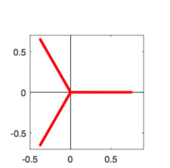
Figure 1. Distributions of the eigenvalues of $M_{n}^{(0)}$ scaled by $n^{4/3}$ for n=200.

Our next result is obtained on the physics level of rigor, i.e., modulo three convergence assumptions which are explicated in the proof of Proposition 2, see § 3. To formulate it, take the family of equations

$$\mathcal{C}^{2}-(x^{2}-A)\mathcal{C}+(x-\beta)=0$$ (1.5)

which we consider as quadratic equations in the variable $\mathcal{C}$ depending on the main variable $x$ and additional parameters $A$ and $\beta$.

Proposition 2.

If $\lim_{n\to\infty}\frac{a_{n}}{n^{2/3}}=A\neq 0$, then (under three additional convergence assumptions given in the proof) the sequence $\{\mu_{n}^{(a_{n})}\}$ of eigenvalue-counting measures for the sequence of matrices $\{\frac{1}{n^{4/3}}M_{n}^{(a_{n})}\}$ weakly converges to a special compactly supported probability measure $\nu_{A}$.

In particular, the support of $\nu_{A}$ consists of all values of the spectral parameter $\beta$ for which there exists a compactly supported in the $x$-plane probability measure $\kappa$ whose Cauchy transform $\mathcal{C}_{\kappa}(x)$ satisfies (1.5) in this plane almost everywhere.

Remark 1.

Numerical experiments and some theoretical considerations indicate that if $\lim_{n\to\infty}\frac{a_{n}}{n^{2/3}}$ does not exist then there is no non-trivial limiting behavior of the spectrum. We think that for $\lim_{n\to\infty}\frac{|a_{n}|}{n^{2/3}}=+\infty$, one can rigorously prove the latter observation. However we are not trying to pursue this aspect in the present paper.

Remark 2.

To make the paper self-contained, let us recall that for a complex-valued measure $\mu$ compactly supported in $\mathbb{C}$, its logarithmic potential is defined as

$$\mathfrak{u}_{\mu}(x):=\int_{\mathbb{C}}\ln|x-\xi|d\mu(\xi)$$

and its Cauchy transform is defined as

$$\mathcal{C}_{\mu}(x):=\int_{\mathbb{C}}\frac{d\mu(\xi)}{x-\xi}=\frac{\mathfrak{\partial}\mathfrak{u}_{\mu}(x)}{\partial x}.$$

Remark 3.

The existence of a signed (real, but not necessarily positive) measure $\mu$ whose Cauchy transform $\mathcal{C}_{\mu}(x)$ satisfies (1.5) almost everywhere in $\mathbb{C}$ is closely related to the properties of the family of quadratic differentials

$$\Psi_{A,\beta}=-((x^{2}-A)^{2}-4(x-\beta))dx^{2}$$ (1.6)

depending on parameters $A$ and $\beta$. We will present some information about this connection in § 3. (For an accessible introduction to quadratic differentials, see e.g. [25]).

1.2. Asymptotic distribution of the branching points of $Sp_{n}(a,\lambda)$ and Yablonskii-Vorob’ev polynomials

To finish the introduction, let us formulate a number of conjectures supported by extensive numerical experiments. For a given positive integer $n$, denote by $\Sigma_{n}$ the set of all branching points of the projection of the algebraic curve $\Gamma_{n}(a):\{Sp_{n}(a,\lambda)=0\}$ to the $a$-axis. In other words, $\Sigma_{n}$ is the set of all values of the complex parameter $a$ for which the matrix $M_{n}^{(a)}$ has a multiple eigenvalue, i.e., $Sp_{n}(a,\lambda)$ has a multiple root. In physics literature such points are called level crossings. Obviously, one can describe $\Sigma_{n}$ as the zero locus of the univariate discriminant polynomial $D_{n}(a)$ which is the resultant of $Sp_{n}(a,\lambda)$ and $\frac{\partial Sp_{n}(a,\lambda)}{\partial\lambda}$ with respect to $\lambda$. One can show that the degree of $D_{n}(a)$ equals $\binom{n+1}{2}$.

Further recall that Yablonskii-Vorob’ev polynomials $\{Q_{n}\}$ are defined as follows, see e.g. [28, 29]. Set $Q_{0}=1,\;Q_{1}=t$, and for $n\geq 1$, define

$$Q_{n+1}=\frac{t\cdot Q_{n}^{2}-4(Q_{n}\cdot Q^{\prime\prime}_{n}-(Q^{\prime}_{n})^{2})}{Q_{n-1}}.$$

Although the latter expression a priori determines a rational function, $Q_{n}$ is in fact a polynomial of degree $\binom{n+1}{2}$, see e.g. [27]. The importance of Yablonskii-Vorob’ev polynomials is explained by the fact that all rational solutions of the second Painlevé equation

$$u_{tt}=tu+2u^{3}+\alpha,\alpha\in\mathbb{C},$$

are presented in the form

$$u(t)=u(t;n)=\frac{d}{dt}\left\{\ln\left[\frac{Q_{n-1}(t)}{Q_{n}(t)}\right]\right\},\;u(t,0)=0,\;u(t;-n):=-u(t;n).$$

Denote by $\mathcal{Z}_{n}$ the zero locus of $Q_{n}$. (Good exposition of the properties of $Q_{n}$ together with several pictures of $\mathcal{Z}_{n}$ can be found in [11]). Our conjectures below reveal an unexpected connection of $\Sigma_{n}$ and $\mathcal{Z}_{n}$.

Remark 4.

One can show that the maximal absolute value of points in $\mathcal{Z}_{n}$ grows as $\frac{3}{\root 3 \of{2}}n^{2/3}$, see [9] and § 5. Similarly, the maximal absolute value of points in $\Sigma_{n}$ grows as $\frac{3}{\root 3 \of{4}}n^{2/3}$, see Lemma 5 and Corollary 2 below.

Conjecture 1.

Given a positive integer $\ell$, define $\Upsilon_{\ell}:=\Sigma_{3\ell}\cup\Sigma_{3\ell+1}\cup\Sigma_{3\ell+2}$. For $R>0$, let $K_{R}$ be the square with the side $2R$ centered at the origin. Then for any fixed $R>0$ and $\ell\to\infty$, the points in $\Upsilon_{\ell}$ converge inside $K_{R}$ to the nodes of a certain fixed hexagonal lattice.

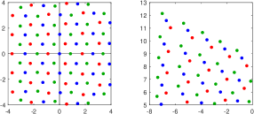
Figure 2. The points of $\Upsilon_{5}$ inside the square $K_{4}$ (left) and close to the upper left corner (right). The points of $\Sigma_{15}$ are shown in red, $\Sigma_{16}$ in blue, and $\Sigma_{17}$ in green.

Conjecture 2.

Set $\widetilde{\Sigma}_{n}=\root{3} \of{2}\cdot\Sigma_{n}$, i.e., multiple every point in $\Sigma_{n}$ by $\root{3} \of{2}$. Then every point in $\widetilde{\Sigma}_{n}$ lies very close to the unique point in $-\mathcal{Z}_{n}$ and vice versa, see Fig. 3. Fixing $n$, define $d(n):=max_{p\in\widetilde{\Sigma}_{n}}\min_{q\in-\mathcal{Z}_{n}}d(p,q)$, i.e., $d(n)$ is the maximal distance between points in $\widetilde{\Sigma}_{n}$ and their respective nearest points in $-\mathcal{Z}_{n}$.

The sequence $\{d(n)\}$ is very slowly growing with $n$, see Example 1 below. It might even have a limit when $n\to\infty$. Moreover for any fixed $R>0$, the sequence $d_{R}(n)$ converges to $0$ where $d_{R}(n)$ is a similar maximin of the pairwise distances taken over all points in $\widetilde{\Sigma}_{n}$ and $-\mathcal{Z}_{n}$ which lie inside the square $K_{R}$.

Example 1.

Numerical experiments show that for $n=10,15,20,25,30,35,40$, the corresponding values of $d(n)$ are approximately $0.03016,0.04160,0.051156,0.05837,$ $0.06378,0.06863,0.07272$ respectively.

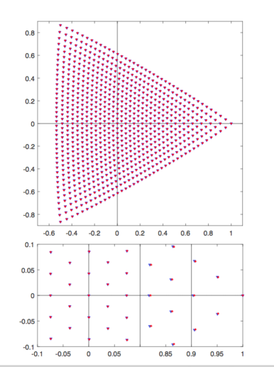
Figure 3. The set $\Sigma_{40}$ of the branching points for $Sp_{40}(a,\lambda)$ together with the zero locus $-{\mathcal{Z}}_{40}$ after scaling sending the three corners to the cubic roots of $1$. The blue dots are the scaled roots of $-{\mathcal{Z}}_{40}$ while the red ones are the scaled branching points of $Sp_{40}(a,\lambda)$. The bottom picture shows a fragment of the top one with substantial magnification. (Observe the surprising closeness; the distinction is hardly visible by a naked eye!)

For illustration of Conjecture 2 see Figure 3. We hope that considerations similar to that in [17, 18] can help to settle it.

Conjecture 3.

When $n\to\infty$, the points in the sequences $\frac{\root{3} \of{4}}{3n^{2/3}}\{\Sigma_{n}\}$ and $\{-\frac{\root{3} \of{2}}{3n^{2/3}}{\mathcal{Z}}_{n}\}$ asymptotically fill the same curvilinear triangular shape $\mathfrak{F}$, see Fig 3.

The interior of $\mathfrak{F}$ consists of all values $a\in\mathbb{C}$ for which the support of measure $\nu_{a}$ introduced in Proposition 2 is a tripod, i.e., consists of three smooth segments with a common point, see Figure 8 (left).

The complement of $\mathfrak{F}$ consists of all values $a\in\mathbb{C}$ for which the support of $\nu_{a}$ is a single smooth segment, see Figure 8 (down). The boundary of $\mathfrak{F}$ consists of those $a\in\mathbb{C}$ for which the support of $\nu_{a}$ is a single curve with a singular point, i.e., $a$ belongs to the boundary between the domain where this support is a tripod and the domain where the support is a smooth single curve, see Figure 8 (right).

Conjecture 3 complements Conjecture 2. For the sequence $\{{\mathcal{Z}}_{n}\}$ parts of the latter conjecture have been settled in [9], see also [3].

Remark 5.

Data sharing not applicable to this article as no datasets were generated or analysed during the current study.

Acknowledgements. The authors are sincerely grateful to M. Duits, A. Kuijlaars, and A. Gabrielov for discussions. The first author wants to thank F. Štampach for his help with the complex version of the main result of [16] and Nuclear Physics Institute at Řež near Prague for the hospitality. The first author is partially supported by International Laboratory of Cluster Geometry NRU HSE, RF Government grant, ag. № 075-15-2021-608 from 08.06.2021. The second author was supported by the Czech Science Foundation (GAČR) within the project 21-07129S. We are very thankful to our anonymous referees for their careful reading of the original submission and a large number of useful suggestions.

2. Case $\lim_{n\to\infty}\frac{a_{n}}{n^{2/3}}=0$. Proof of Theorem 1

Let us start our considerations of the spectral asymptotic of sequences $\{M_{n}^{(a_{n})}\}$ with the simplest case $a_{n}=0,\;n=1,2,3,\dots$.

Proposition 3.

(i) The sequence $Sp_{n}(0,\lambda)$ splits into the following three subsequences:

1. for $n+1=3\ell$, the polynomial $Sp_{n}(0,\lambda)$ contains only the powers of $\lambda$ divisible by $3$; i.e., we have $Sp_{n}(0,\lambda)=u^{(\ell)}(\lambda^{3})$;

2. for $n+1=3\ell+1$, one has $Sp_{n}(0,\lambda)=\lambda v^{(\ell)}(\lambda^{3})$;

3. for $n+1=3\ell+2$, one has $Sp_{n}(0,\lambda)=\lambda^{2}w^{(\ell)}(\lambda^{3})$,

where $u^{(\ell)}(\xi),v^{(\ell)}(\xi)$, and $w^{(\ell)}(\xi)$ are polynomials of degree $\ell$ in the variable $\xi$.

(ii) All three polynomials $u^{(\ell)}(\xi),v^{(\ell)}(\xi),w^{(\ell)}(\xi)$ have simple and negative roots.

Corollary 1.

(a) The spectrum of $M_{n}^{(0)},$ i.e., the zero locus of $Sp_{n}(0,\lambda)$, is invariant under the rotation by the angle $2\pi/3$ around the origin.

(b) For any positive integer $n$, the spectrum of $M_{n}^{(0)}$ is located on the union of the three rays through the origin as illustrated in Figure 1.

To prove Proposition 3 following the ideas of [16], we need to introduce a double indexed polynomial sequence containing our original sequence of characteristic polynomials $\{Sp_{n}(0,\lambda)\}$. The most natural way to do this is to consider the principal minors of $M_{n}^{(0)}-\lambda I$ given by:

$$M_{n}^{(0)}-\lambda I:=\left(\begin{matrix}-\lambda&0&2&0&0&\cdots&0\\ n&-\lambda&0&6&0&\cdots&0\\ 0&n-1&-\lambda&0&12&\cdots&0\\ \vdots&\vdots&\ddots&\ddots&\ddots&\ddots&\vdots\\ 0&0&\cdots&3&-\lambda&0&n(n-1)\\ 0&0&\cdots&0&2&-\lambda&0\\ 0&0&\cdots&0&0&1&-\lambda\end{matrix}\right).$$ (2.1)

Namely, denote by $\Delta_{n}^{(k)}(\lambda)$ the $k$-th principal minor of (2.1). Then

$$Sp_{n}(0,\lambda)=\Delta_{n}^{(n+1)}(\lambda)=\det(M_{n}^{(0)}-\lambda I).$$

Since the latter matrix is $4$-diagonal with one subdiagonal and two superdiagonals, then, by a general result of [21], its principal minors satisfy a $4$-term linear recurrence relation. Simple explicit calculation gives

$$\Delta_{n}^{(k)}(\lambda)=-\lambda\Delta_{n}^{(k-1)}(\lambda)+(n-k+2)(n-k+3)(k-1)(k-2)\Delta_{n}^{(k-3)}(\lambda),$$ (2.2)

where $n$ is fixed and $k$ runs from $1$ to $n+1,$ with the standard initial conditions

$$\Delta_{n}^{(-2)}(\lambda)=\Delta_{n}^{(-1)}(\lambda)=0,\quad\Delta_{n}^{(0)}(\lambda)=1.$$

Notice that recurrence (2.2) has variable coefficients depending both on $k$ and $n$.

Another form of (2.2) which is a bit easier to study is as follows. To simplify our manipulations with the signs, let us instead of $M_{n}^{(0)}-\lambda I$ consider the principal minors of $M_{n}^{(0)}+\lambda I$. Introducing $\nabla_{n}^{(k)}(\lambda):=\Delta_{n}^{(k)}(-\lambda)$, we get the recurrence:

$$\nabla_{n}^{(k)}(\lambda)=\lambda\nabla_{n}^{(k-1)}(\lambda)+(n-k+2)(n-k+3)(k-1)(k-2)\nabla_{n}^{(k-3)}(\lambda)$$ (2.3)

with the initial conditions

$$\nabla_{n}^{(-2)}(\lambda)=\nabla_{n}^{(-1)}(\lambda)=0,\quad\nabla_{n}^{(0)}(\lambda)=1.$$

Lemma 4.

Set $\nabla_{n}^{(3j)}(\lambda)=U_{n}^{(j)}(\xi)$, $\nabla_{n}^{(3j+1)}(\lambda)=\lambda V_{n}^{(j)}(\xi)$, $\nabla_{n}^{(3j+2)}(\lambda)=\lambda^{2}W_{n}^{(j)}(\xi)$, where $\xi=\lambda^{3}$ and $U_{n}^{(j)},V_{n}^{(j)},W_{n}^{(j)}$ are monic polynomials of degree $j$.

Using $U_{n}^{(j)},V_{n}^{(j)},W_{n}^{(j)}$, recurrence (2.3) can be rewritten as the system:

$$\begin{cases}U_{n}^{(j)}(\xi)=\xi W_{n}^{(j-1)}(\xi)+(n-3j+2)(n-3j+3)(3j-2)(3j-1)U_{n}^{(j-1)}(\xi)\\ V_{n}^{(j)}(\xi)=U_{n}^{(j)}(\xi)+(n-3j+1)(n-3j+2)(3j-1)3j\,V_{n}^{(j-1)}(\xi)\\ W_{n}^{(j)}(\xi)=V_{n}^{(j)}(\xi)+(n-3j)(n-3j+1)3j(3j+1)W_{n}^{(j-1)}(\xi)\ \end{cases}$$ (2.4)

with the initial conditions $U_{n}^{(0)}(\xi)=V_{n}^{(0)}(\xi)=W_{n}^{(0)}(\xi)=1$ where for any fixed $n$, $j$ runs from $1$ to $[n/3]$.

Proof.

Simple algebra. ∎

Proof of Proposition 3.

Item (i) follows immediately from Lemma 4. While proving item (ii) of Proposition 3, we will use notation of Lemma 4. Notice that polynomials $U_{n}^{(\ell)}$, $V_{n}^{(\ell)}$, $W_{n}^{(\ell)}$ coincide up to the change of sign of the variable $\xi$ with polynomials $u^{(\ell)},$ $v^{(\ell)}$ and $w^{(\ell)}$ respectively.

We need to show that for any positive integer $n$, each polynomial in the recurrence (2.4) has positive coefficients and real negative roots. Moreover the roots of any two consecutive polynomials in each of the three sequences $\{U_{n}^{(j)}\}_{j=0}^{[n/3]}$, $\{V_{n}^{(j)}\}_{j=0}^{[n/3]}$, $\{W_{n}^{(j)}\}_{j=0}^{[n/3]}$ are strictly interlacing and are therefore simple.

Positivity of the coefficients of polynomials is straightforward from the positivity of coefficients in (2.4) and the initial conditions. Let us settle the negativity of all roots by using induction on $j$. For $j=1$ and $n\geq 3$, it is trivial to check that the negative root of the $U_{n}^{(1)}$ is larger than that of $V_{n}^{(1)}$ which is larger than that of $W_{n}^{(1)}$.

Let us consider the case $j=2$. Note that $U_{n}^{(2)}=\xi W_{n}^{(1)}+20(n-4)(n-3)U_{n}^{(1)}$. Elementary calculations give $\xi W_{n}^{(1)}=\xi^{2}+(84-8n+20n^{2})\xi$ and $U_{n}^{(1)}=\xi-2n+2n^{2}$, which implies that the two roots of $\xi W_{n}^{(1)}$ are non-positive and the only root of $U_{n}^{(1)}$ is located strictly between them for $n\geq 3$. Hence, then using Lemma 1.10 of [14] or conducting elementary calculations, we can conclude that $U_{n}^{(2)}$ has simple negative roots for $n\geq 3$. Using similar elementary calculations we obtain similar results for the pair $U_{n}^{(2)},V_{n}^{(1)}$ implying that $V_{n}^{(2)}$ has simple negative roots and for the pair $V_{n}^{(2)},W_{n}^{(1)}$ implying that $W_{n}^{(2)}$ has simple negative roots.

Assume now that our hypothesis holds for a given positive integer $j$. Note that, in each of the three equations in (2.4), the degree of the first polynomial in the right-hand side is bigger than the degree of the second polynomial by one. This indicates that the largest root belongs to the polynomial with the larger degree. Furthermore by Corollary 1.30 of [14], we can derive the following results:

$$\xi W_{j-1}\leftarrow U_{j}\leftarrow U_{j-1}$$ (2.5)

$$U_{j}\leftarrow V_{j}\leftarrow V_{j-1}$$ (2.6)

$$V_{j}\leftarrow W_{j}\leftarrow W_{j-1}.$$ (2.7)

Here the arrow $"\leftarrow``$ indicates that the corresponding pair of polynomials have simple interlacing roots with the largest root belonging to the polynomial at which the arrow points.

1. Consider the recurrence

   $$U_{n}^{(j+1)}=\xi W_{n}^{(j)}+(n-3j-1)(n-3j)(3j+1)(3j+2)U_{n}^{(j)}.$$

   We can rewrite $\xi W_{n}^{(j)}$ as $\xi V_{n}^{(j)}+(n-3j)(n-3j+1)3j(3j+1)\xi W_{n}^{(j-1)}.$ Observe that $\xi W_{n}^{(j-1)}\leftarrow U_{n}^{(j)}$ by induction hypothesis and Corollary 1.30 in [14]. Using (2.2), we can conclude that $\xi V_{n}^{(j)}\leftarrow U_{n}^{(j)}$ since all roots of $U_{n}^{(j)}$ are negative and simple. Hence $\xi W_{n}^{(j)}\leftarrow U_{n}^{(j)}$, by Lemma 1.31 in [14]. Therefore $U_{n}^{(j+1)}$ has real and simple roots, by Lemma 1.10 in [14].

2. Consider the recurrence

   $$V_{n}^{(j+1)}=U_{n}^{(j+1)}+(n-3j-2)(n-3j-1)(3j+2)(3j+3)V_{n}^{(j)}.$$

   One can rewrite $U_{n}^{(j+1)}$ as given in part $(a)$ above. By (2.2), $U_{n}^{(j)}\leftarrow V_{n}^{(j)}$ and by (2.3), $\xi W_{n}^{(j)}\leftarrow V_{n}^{(j)}$ since $W_{n}^{(j)}$ and $V_{n}^{(j)}$ only have negative and simple roots. Proof is concluded by the same argument as in part $(a)$.

3. Consider the recurrence

   $$W_{n}^{(j+1)}=V_{n}^{(j+1)}+(n-3j-3)(n-3j-2)(3j+3)(3j+4)W_{n}^{(j)}.$$

   One can rewrite $V_{n}^{(j+1)}$ as in part $(b)$. By (2.3), $V_{n}^{(j)}\leftarrow W_{n}^{(j)}$. $U_{n}^{(j+1)}\leftarrow W_{n}^{(j)}$ by part $(a)$, Corollary 1.30 in [14] and the fact that both $U_{n}^{(j+1)}$ and $W_{n}^{(j)}$ have only negative and simple roots. Proof is concluded by the same argument as in parts $(a)$ and $(b)$.

∎

Let us now settle Theorem 1 in the special case $a_{n}=0;\;n=1,2,3,\dots$.

Proof.

In order to apply the approach of [16], we need the variable recurrence coefficients to stabilize when $\frac{k}{n}\to\tau$, for any fixed $\tau\in[0,1]$. To get such stabilization, consider the rescaled matrix

$$\frac{1}{n^{4/3}}M_{n}^{(0)}-\beta I:=\left(\begin{matrix}-\beta&0&\frac{2}{n^{4/3}}&0&0&\cdots&0\\ \frac{n}{n^{4/3}}&-\beta&0&\frac{6}{n^{4/3}}&0&\cdots&0\\ 0&\frac{n-1}{n^{4/3}}&-\beta&0&\frac{12}{n^{4/3}}&\cdots&0\\ \vdots&\vdots&\ddots&\ddots&\ddots&\ddots&\vdots\\ 0&0&\cdots&\frac{3}{n^{4/3}}&-\beta&0&\frac{n(n-1)}{n^{4/3}}\\ 0&0&\cdots&0&\frac{2}{n^{4/3}}&-\beta&0\\ 0&0&\cdots&0&0&\frac{1}{n^{4/3}}&-\beta\end{matrix}\right)$$ (2.8)

which is obtained from the matrix $M_{n}^{(0)}-\lambda I$ defined in (2.1) dividing it by $n^{4/3}$ and setting $\beta=n^{-4/3}\lambda$. Denote by $\widetilde{\Delta}_{n}^{(k)}(\beta)$ the $k$-th principal minor of the above matrix. Thus, we get $\widetilde{\Delta}_{n}^{(k)}(\beta):=\Delta_{n}^{(k)}(n^{4/3}\beta)/n^{4k/3}$. The sequence $\{\widetilde{\Delta}_{n}^{(k)}(\beta)\}_{k=1}^{n+1}$ satisfies the scaled recurrence

$$\widetilde{\Delta}_{n}^{(k)}(\beta)=-\beta\widetilde{\Delta}_{n}^{(k-1)}(\beta)+\frac{(n-k+2)(n-k+3)(k-1)(k-2)}{n^{4}}\widetilde{\Delta}_{n}^{(k-3)}(\beta),$$ (2.9)

obtained from (2.2) by substituting $\beta=n^{-4/3}\lambda$. In other words, (2.9) is satisfied by the characteristic polynomials of the principal minors of the matrix $\frac{1}{n^{4/3}}M_{n}^{(0)}$. Then when $\frac{k}{n}\to\tau,$ the latter recurrence transforms into the recurrence:

$$\Omega_{\tau}^{(k)}(\beta)=-\beta\Omega_{\tau}^{(k-1)}(\beta)+(1-\tau)^{2}\tau^{2}\Omega_{\tau}^{(k-3)}(\beta)$$ (2.10)

with constant coefficients. The polynomial $\Omega_{\tau}^{(k)}(\beta)$ can be interpreted at the $k$-th principal minor of the infinite Toeplitz matrix

$$\left(\begin{matrix}-\beta&0&\tau^{2}&0&0&\cdots&0\\ (1-\tau)&-\beta&0&\tau^{2}&0&\cdots&0\\ 0&(1-\tau)&-\beta&0&\tau^{2}&\cdots&0\\ \vdots&\vdots&\ddots&\ddots&\ddots&\ddots&\vdots\\ 0&0&\cdots&(1-\tau)&-\beta&0&\tau^{2}\\ 0&0&\cdots&0&(1-\tau)&-\beta&0\\ 0&0&\cdots&0&0&(1-\tau)&-\beta\end{matrix}\right).$$ (2.11)

Following [16] and using Proposition 3, we conclude that the Cauchy transform of the asymptotic root-counting measure for the polynomial sequence

$$\left\{Sp_{n}(0,\beta n^{4/3})\right\}=\left\{n^{\frac{4(n+1)}{3}}\cdot\widetilde{\Delta}_{n}^{(n+1)}(\beta)\right\}$$

is obtained by averaging the Cauchy transforms of the asymptotic distributions of (2.10) over $\tau\in[0,1]$.

In fact, in the case under consideration even the density of the former distribution can be obtained by averaging the densities of the latter family of distributions which we can confirm as follows.

Recurrence (2.10) is similar to the one considered in the last section of [4] and has very nice asymptotic distribution of its roots, see Figure 4. Observe that for any $\tau\in[0,1],$ the initial conditions for (2.10) are given by

$$\Omega_{\tau}^{(-2)}(\beta)=\Omega_{\tau}^{(-1)}(\beta)=0,\;\Omega_{\tau}^{(0)}(\beta)=1.$$

Since (2.10) has constant coefficients, the support of the asymptotic root-counting measure of its solution is described by the well-known result of Beraha-Cahane-Weiss [2]. Namely, this support coincides with the set of all $\beta\in\mathbb{C}$ such that among three solutions of the characteristic equation

$$\Psi^{3}+\beta\Psi^{2}-(1-\tau)^{2}\tau^{2}=0$$ (2.12)

with respect to the variable $\Psi$ two have the same modulus which is bigger or equal to the modulus of the third solution of (2.12). From considerations of [4] one can easily derive that, for any fixed $\tau\in[0,1],$ this support is the union of three intervals starting at the origin and ending at the branching points of (2.12), i.e., those values of $\beta$ and $\tau$ for which (2.12) has a multiple root with respect to $\Psi$. The latter branching points are given by the equation:

$$\beta^{3}=\frac{27}{4}(1-\tau)^{2}\tau^{2}$$ (2.13)

and their location for three values of $\tau$ is shown in Figure 4. Observe that if for $\tau\in[0,1]$, we denote the branching point lying on the positive half-axis by $\beta^{+}(\tau)$, then it attains its maximal value when $\tau=1/2$ and this maximum equals $\frac{3}{4}$.

As we mentioned before, in the case under consideration for any $\tau\in[0,1]$, the roots of all polynomials generated by (2.10) lie on three fixed rays through the origin. Therefore, the density of the asymptotic root-counting measure of the polynomial sequence

$$\left\{Sp_{n}(0,\beta n^{4/3})\right\}=\left\{n^{{\frac{4(n+1)}{3}}}\widetilde{\Delta}_{n}^{(n+1)}(\beta)\right\}$$

is obtained by averaging the densities of (2.10) over $\tau\in[0,1]$, cf. [12] and [16]. Therefore, the support of the asymptotic root distribution for $\{Sp_{n}(0,\beta n^{4/3})\}$ in the $\beta$-plane is the union of three intervals of length $\frac{3}{4}$. ∎

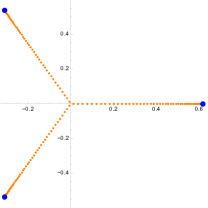
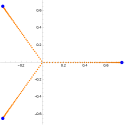
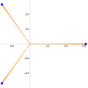
Figure 4. Roots of $\Omega_{\tau}^{(150)}(\beta)$ for $\tau=1/4$, $\tau=1/2$, $\tau=3/4$. Endpoints of the segments are the branching points given by (2.13) for the respective values of parameter $\tau$.

Proof of Theorem 1 in case when $\lim_{n\to\infty}\frac{a_{n}}{n^{2/3}}=0$,.

We need to show that Proposition 3 holds asymptotically for any sequence $\{a_{n}\}$ of complex numbers satisfying the condition

$$\lim_{n\to\infty}\frac{a_{n}}{n^{2/3}}=0.$$

Indeed, the principal minors of the matrix

$$M_{n}^{(a_{n})}-\lambda I:=\left(\begin{matrix}-\lambda&a_{n}&2&0&0&\cdots&0\\ n&-\lambda&2a_{n}&6&0&\cdots&0\\ 0&n-1&-\lambda&3a_{n}&12&\cdots&0\\ \vdots&\vdots&\ddots&\ddots&\ddots&\ddots&\vdots\\ 0&0&\cdots&3&-\lambda&(n-1)a_{n}&n(n-1)\\ 0&0&\cdots&0&2&-\lambda&na_{n}\\ 0&0&\cdots&0&0&1&-\lambda\end{matrix}\right),$$ (2.14)

satisfy the recurrence

$$\Delta_{n}^{(k)}(a_{n},\lambda)=-\lambda\Delta_{n}^{(k-1)}(a_{n},\lambda)+(k-1)(n-k+2)a_{n}\Delta_{n}^{(k-2)}(a_{n},\lambda)$$

$$+(n-k+2)(n-k+3)(k-1)(k-2)\Delta_{n}^{(k-3)}(a_{n},\lambda),$$ (2.15)

where $k=1,2,\dots,n+1,$ with the initial conditions

$$\Delta_{n}^{(-2)}(a_{n},\lambda)=\Delta_{n}^{(-1)}(a_{n},\lambda)=0,\quad\Delta_{n}^{(0)}(a_{n},\lambda)=1.$$

To obtain a converging sequence of root-counting measures one has to consider the scaled matrix $\frac{1}{n^{4/3}}M_{n}^{(a_{n})}-\beta I$ given by:

$$\left(\begin{matrix}-\beta&\frac{a_{n}}{n^{4/3}}&\frac{2}{n^{4/3}}&0&0&\cdots&0\\ \frac{n}{n^{4/3}}&-\beta&\frac{2a_{n}}{n^{4/3}}&\frac{6}{n^{4/3}}&0&\cdots&0\\ 0&\frac{n-1}{n^{4/3}}&-\beta&\frac{3a_{n}}{n^{4/3}}&\frac{12}{n^{4/3}}&\cdots&0\\ \vdots&\vdots&\ddots&\ddots&\ddots&\ddots&\vdots\\ 0&0&\cdots&\frac{3}{n^{4/3}}&-\beta&\frac{(n-1)a_{n}}{n^{4/3}}&\frac{n(n-1)}{n^{4/3}}\\ 0&0&\cdots&0&\frac{2}{n^{4/3}}&-\beta&\frac{na_{n}}{n^{4/3}}\\ 0&0&\cdots&0&0&\frac{1}{n^{4/3}}&-\beta\end{matrix}\right).$$ (2.16)

It is obtained by dividing (2.14) by $n^{4/3}$ and setting $\beta=\lambda/n^{4/3}$. Its principal minors satisfy the recurrence

$$\widetilde{\Delta}_{n}^{(k)}(a_{n},\beta)=-\beta\widetilde{\Delta}_{n}^{(k-1)}(a_{n},\beta)-\frac{(k-1)(n-k+2)a_{n}}{n^{8/3}}\widetilde{\Delta}_{n}^{(k-2)}(a_{n},\beta)$$

$$+\frac{(n-k+2)(n-k+3)(k-1)(k-2)}{n^{4}}\widetilde{\Delta}_{n}^{(k-3)}(a_{n},\beta).$$ (2.17)

Since $\lim_{n\to\infty}\frac{a_{n}}{n^{2/3}}=0$, then for $\frac{k}{n}\to\tau,$ the family (2.17) of recurrence relations converges to the earlier family (2.10) corresponding to the case $a_{n}=0,\;n=1,2,3,\dots$. Therefore the measure obtained by averaging the family of root-counting measures for recurrence relations with constant coefficients is exactly the same as in the previous case $a_{n}=0$, i.e., it coincides with $\nu_{0}$. Additionally observe that by a general result of [16], the support of the asymptotic root-counting measure of the sequence $\{\widetilde{\Delta}_{n}^{(k)}(a_{n},\beta)\}$ can only be smaller than that of $\nu_{0}$ and their Cauchy transforms must coincide outside the support of $\nu_{0}$. Since the support of $\nu_{0}$ is the union of three straight intervals through the origin the resulting asymptotic root-counting measure for the sequence $\{Sp_{n}(a_{n},\beta n^{4/3})\}$ in case $\lim_{n\to\infty}\frac{a_{n}}{n^{2/3}}=0$ coincides with $\nu_{0}$ as well. ∎

Remark 6.

Since the support of the limiting measure $\nu_{0}$ consists of three segments through the origin it is in principle possible to find integral formulas for the density and the Cauchy transform of $\nu_{0}$ similar to those presented in [16], [12] and [23]. In particular, in the complement to the support of $\nu_{0}$, its Cauchy transform is given by

$$\mathcal{C}_{\nu_{0}}(\beta)=\int_{0}^{1}\frac{\partial}{\partial\beta} \left(\log\tilde{\Psi}\right){d\tau},$$

where $\tilde{\Psi}$ is the unique solution of (2.12) satisfying $\lim_{\beta\to\infty}\frac{\tilde{\Psi}}{\beta}=-1$. However it seems difficult to find either a somewhat explicit expression for $\mathcal{C}_{\nu_{0}}(\beta)$ or a linear differential operator with polynomial coefficients annihilating $\mathcal{C}_{\nu_{0}}(\beta)$. (Observe that such an operator always exists since $\mathcal{C}_{\nu_{0}}(\beta)$ belongs to the Nilsson class, see [20]).

3. Case $\lim_{n\to\infty}\frac{a_{n}}{n^{2/3}}=A\neq 0$.

3.1. “Proof” of Proposition 2

Similarly to the previous section, let $\Delta^{(k)}_{n}(a_{n},\lambda)$ be the characteristic polynomial of the $k$-th principal minors of $M_{n}^{(a_{n})}$, see (1.4). As in the previous section let us start with a special sequence $\{a_{n}=An^{2/3}\}$ for some fixed $A\neq 0$. Next consider the matrix

$$M_{n}^{(An^{2/3})}-\lambda I:=\left(\begin{matrix}-\lambda&An^{2/3}&2&0&0&\cdots&0\\ n&-\lambda&2An^{2/3}&6&0&\cdots&0\\ 0&n-1&-\lambda&3An^{2/3}&12&\cdots&0\\ \vdots&\vdots&\ddots&\ddots&\ddots&\ddots&\vdots\\ 0&0&\cdots&3&-\lambda&(n-1)An^{2/3}&n(n-1)\\ 0&0&\cdots&0&2&-\lambda&nAn^{2/3}\\ 0&0&\cdots&0&0&1&-\lambda\end{matrix}\right).$$ (3.1)

and denote its $k$-th principal minor by $\Delta_{n}^{(k)}(An^{2/3},\lambda)$. This sequence of minors satisfies the recurrence relation of length $4$ of the form:

$$\Delta_{n}^{(k)}(An^{2/3},\lambda)=-\lambda\Delta_{n}^{(k-1)}(An^{2/3},\lambda)-(k-1)(n-k+2)An^{2/3}\Delta^{(k-2)}_{n}(An^{2/3},\lambda)$$

$$+(n-k+2)(n-k+3)(k-1)(k-2)\Delta_{n}^{(k-3)}(An^{2/3},\lambda).$$

To get stabilization similar to that of § 2, introduce the scaled matrix

$$\frac{1}{n^{4/3}}M_{n}^{(An^{2/3})}-\beta I:=\left(\begin{matrix}-\beta&\frac{A}{n^{2/3}}&\frac{2}{n^{4/3}}&0&0&\cdots&0\\ \frac{n}{n^{4/3}}&-\beta&\frac{2A}{n^{2/3}}&\frac{6}{n^{4/3}}&0&\cdots&0\\ 0&\frac{n-1}{n^{4/3}}&-\beta&\frac{3A}{n^{2/3}}&\frac{12}{n^{4/3}}&\cdots&0\\ \vdots&\vdots&\ddots&\ddots&\ddots&\ddots&\vdots\\ 0&0&\cdots&\frac{3}{n^{4/3}}&-\beta&\frac{(n-1)A}{n^{2/3}}&\frac{n(n-1)}{n^{4/3}}\\ 0&0&\cdots&0&\frac{2}{n^{4/3}}&-\beta&\frac{nA}{n^{2/3}}\\ 0&0&\cdots&0&0&\frac{1}{n^{4/3}}&-\beta\end{matrix}\right)$$ (3.2)

where $\beta=\lambda n^{-4/3}$.

Its principal minors (which we denote by $\widetilde{\Delta}_{n}^{(k)}(An^{2/3},\beta)$) satisfy the relation

$$\widetilde{\Delta}_{n}^{(k)}(An^{2/3},\beta)=-\beta\widetilde{\Delta}_{n}^{(k-1)}(An^{2/3},\beta)-\frac{(k-1)(n-k+2)A}{n^{2}}\widetilde{\Delta}_{n}^{(k-2)}(An^{2/3},\beta)$$

$$+\frac{(n-k+2)(n-k+3)(k-1)(k-2)}{n^{4}}\widetilde{\Delta}_{n}^{(k-3)}(An^{2/3},\beta).$$ (3.3)

Assuming that $\frac{k}{n}\to\tau,$ we obtain that (3.1) tends to the following relation with constant coefficients:

$$\Omega_{\tau}^{(k)}(A,\beta)=-\beta\Omega_{\tau}^{(k-1)}(A,\beta)-A\tau(1-\tau)\Omega_{\tau}^{(k-2)}(A,\beta)+(1-\tau)^{2}\tau^{2}\Omega_{\tau}^{(k-3)}(A,\beta),$$ (3.4)

whose characteristic equation is given by

$$\Psi^{3}+\beta\Psi^{2}+A\tau(1-\tau)\Psi-(1-\tau)^{2}\tau^{2}=0.$$ (3.5)

The polynomial $\Omega_{\tau}^{(k)}(A,\beta)$ can be interpreted at the $k$-th principal minor of infinite Toeplitz matrix

$$\left(\begin{matrix}-\beta&A\tau&\tau^{2}&0&0&\cdots&0\\ (1-\tau)&-\beta&A\tau&\tau^{2}&0&\cdots&0\\ 0&(1-\tau)&-\beta&A\tau&\tau^{2}&\cdots&0\\ \vdots&\vdots&\ddots&\ddots&\ddots&\ddots&\vdots\\ 0&0&\cdots&(1-\tau)&-\beta&A\tau&\tau^{2}\\ 0&0&\cdots&0&(1-\tau)&-\beta&A\tau\\ 0&0&\cdots&0&0&(1-\tau)&-\beta\end{matrix}\right).$$ (3.6)

For a generic complex $A$, the union over all $\tau\in[0,1]$ of the supports of the asymptotic root-counting measures $\mu_{A}^{(\tau)}$ for the polynomial sequences $\{\Omega_{\tau}^{(k)}(A,\beta)\}_{k=1}^{\infty}$ (depending on $\tau\in[0,1]$) is strictly larger than that of $\nu_{A}$, see Figure 5. In this case we can only conclude that the corresponding Cauchy transforms of both measures coincide with each other in the complement to the larger support. (This fact follows from the complex version of the main result of [16] corresponded to the first author by A. Kuijlaars, see below). The latter circumstance implies that the measure

$$\mathfrak{M}_{A}=\int_{0}^{1}\mu_{A}^{(\tau)}d\tau$$

is obtained as the balayage of measure $\nu_{A}$. (The above mentioned complex version of the main result of [16] is worked out in details in § 6.)

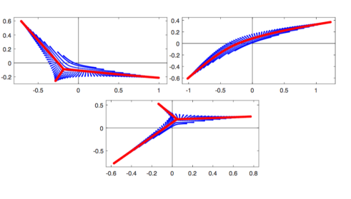
Figure 5. The blue domain is (an approximation to) the union over $\tau\in[0,1]$ of the supports for the asymptotic root-counting measures for the polynomial sequences $\{\Omega_{\tau}^{(k)}(A,\beta)\}$ defined by (3.4). The red curve is the zero locus of $Sp_{200}(An^{2/3},\beta n^{4/3})$. We use $A=(1-i)/2$ (upper left), $A=1+i$ (upper right), and $A=i/2$ (bottom).

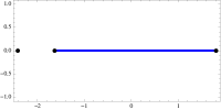
Figure 6. The union over $\tau\in[0,1]$ of the supports of the asymptotic root-counting measures for the sequences $\{\Omega_{\tau}^{(k)}(A,\beta)\}$ in case $A=3$. Black dots are the three branching points given by (3.11).

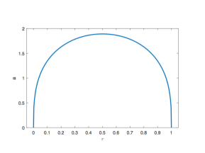
Figure 7. Plot of curve $A^{3}-27\tau+27\tau^{2}=0$ in the real $(A,\tau)$-plane. $A$ is the vertical and $\tau$ is the horizontal axes.

However, the next Lemma shows that in case $A\geq\frac{3}{\root{3} \of{4}}$ (which fits the situation covered by the main result of [12],) these supports coincide and one can obtain the density of $\nu_{A}$ by averaging the densities of (3.4).

Lemma 5.

If $A\geq\frac{3}{\root{3} \of{4}},$ then for any $\tau\in[0,1],$ the support of the asymptotic root-counting measure given by the polynomial sequence defined by (3.4) is a real interval. This interval connects two branching points defined by (3.7).

Proof.

Using the standard expression for the discriminant, one can check that all three branching points of (3.5) with respect to $\Psi$ satisfy the equation:

$$4\beta^{3}+A^{2}\beta^{2}-18A\beta\tau(1-\tau)+\tau(1-\tau)(27\tau^{2}-27\tau-4A^{3})=0.$$ (3.7)

To check that for $A\geq\frac{3}{\root{3} \of{4}},$ and any $\tau\in[0,1],$ all three solutions of (3.7) are real, we calculate the discriminant of (3.7) with respect to $\beta$. Again using symbolic manipulations, we get that this discriminant is given by:

$$Dsc:=16\tau(1-\tau)(A^{3}-27\tau+27\tau^{2})^{3}.$$

For $\tau\in[0,1],$ the graph of $Dsc$ in the real $(A,\tau)$-plane is presented in Figure 7. One can easily check that the maximal value of $A$ on this graph is obtained when $\tau=1/2$ and is equal to $\frac{3}{\root{3} \of{4}}$. This fact implies that $\frac{3}{\root{3} \of{4}}$ is the largest real value of $A$ for which roots of (3.7) w.r.t. $\beta$ can become multiple for some choice of $\tau\in[0,1]$. Moreover checking the location of these roots for some value of $A>\frac{3}{\root{3} \of{4}}$ (for example, for $A=3$ shown in Figure 6) we can conclude that all three roots of (3.7) are real for any $\tau\in[0,1]$. The latter circumstance together with the reality of the situation imply that supports of the asymptotic root counting measure is real for any $\tau\in[0,1]$. ∎

Corollary 2.

The maximal absolute value of points in $\Sigma_{n}$ grows like $\frac{3}{\root{3} \of{4}}n^{2/3}.$

Remark 7.

The special value $A=\frac{3}{\root{3} \of{4}}$ corresponds to the real corner of the asymptotic limiting domain $\mathcal{F}$ appearing in Conjecture 2.

Remark 8.

One can additionally show that for $A\geq\frac{3}{\root{3} \of{4}},$ the union of the supports (which is the union of all real intervals described in Lemma 5 coincides with the interval bounded by the two rightmost branching points given by (3.11), see Fig 6.

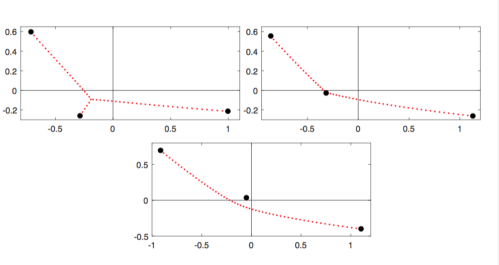
Figure 8. Root distributions of $Sp_{200}(An^{2/3},\beta n^{4/3})$ in the $\beta$-plane for $A=(1-i)/2$ (left), $A=4/5-2i/3$ (right) and $A=2/3-i\;$ (down). Larger dots are the endpoints of the support given by (3.11).

Remark 9.

Similarly to the case $A=0,$ for any $A\geq\frac{3}{\root{3} \of{4}}$, one can represent the Cauchy transform of $\nu_{A}$ as

$$\mathcal{C}_{\nu_{A}}(\beta)=\int_{0}^{1}\frac{\partial}{\partial\beta}\left(\tilde{\Psi}\right)d\tau,$$

in the complement to the support of $\nu_{A}$ (which is an interval explicitly given in Lemma 5). Here $\tilde{\Psi}$ is the unique solution of (3.5) satisfying the condition

$$\lim_{\beta\to\infty}\frac{\tilde{\Psi}}{\beta}=-1.$$

(In an appropriate domain in $\mathbb{C}$ such presentation for the Cauchy transform of $\nu_{A}$ is valid for any complex $A$.)

Let us now discuss Proposition 2.

”Proof“ of Proposition 2 under additional convergence assumptions.

To obtain the support of the limiting measure $\nu_{A}$ whose existence is claimed in the Proposition, we argue as follows. Assume that we have a (sub)sequence $\beta_{j_{n},n}$ of the eigenvalues of the sequence of matrices $\{n^{-4/3}M_{n}^{(An^{2/3})}\}$ (one eigenvalue for each $n$) converging to some finite limit which we denote by $\Lambda$. Denote by $\{p_{n}\}$ the corresponding (sub)sequence of eigenpolynomials of (the sequence of) differential operators $\{T_{n}\}$, see (1.3) in the Introduction. For each $T_{n}$ the value of its parameter $a_{n}$ equals $An^{2/3}$. Then each eigenpolynomial $p_{n}$ satisfies its own differential equation of the form

$$p_{n}^{\prime\prime}-(x^{2}-An^{2/3})p^{\prime}_{n}+(nx-\beta_{j_{n},n}n^{4/3})p_{n}=0.$$ (3.8)

First assumption. We assume that if the subsequence $\{\beta_{j_{n},n}\}$ has a finite limit $\Lambda$, then, after appropriate scaling of $x$, the sequence $\{\mu_{n}\}$ of the root-counting measures of $\{p_{n}\}$ converges in the weak sense to some limiting measure $\kappa_{a,\Lambda}$ whose support consists of finitely many compact curves and points.

This assumption implies that the sequence of appropriately scaled Cauchy transforms of $\{\mu_{n}\}$ converges to the Cauchy transform of the limiting measure $\kappa_{a,\Lambda}$. The appropriate scaling of $x$ which might provide such a convergence can be easy guessed from (3.8). Namely, substituting $x=\Theta n^{1/3}$ and dividing the above equation by $n^{4/3}p_{n}$, we get the relation

$$\frac{\frac{d^{2}p_{n}}{d\Theta^{2}}}{n^{2}p_{n}}-(\Theta^{2}-A)\frac{\frac{dp_{n}}{d\Theta}}{np_{n}}+(\Theta-\beta_{j_{n},n})=0$$ (3.9)

with respect to the new independent variable $\Theta$. Observe that the scaled logarithmic derivative $\frac{1}{n}\frac{d}{d\Theta}(\log p_{n})$ is the Cauchy transform of the root-counting measure of the polynomial $p_{n}(\Theta n^{1/3})$ with respect to the new variable $\Theta$.

Second assumption. Assuming that the sequence $\{\mu_{n}\}$ of the root-counting measures of $\{p_{n}(\Theta n^{1/3})\}$ converges to $\kappa_{a,\Lambda},$ we additionally assume that the sequences of the root-counting measures of its first and second derivatives converge to the same measure $\kappa_{a,\Lambda}.$

(Apparently this assumption can be rigorously proved by using the same arguments as presented in [4].)

Under the above two main assumptions and using (3.9), we get that the Cauchy transform $\mathcal{C}_{A,\Lambda}$ of $\kappa_{A,\Lambda}$ satisfies the quadratic equation:

$$\mathcal{C}_{A,\Lambda}^{2}-(\Theta^{2}-A)\mathcal{C}_{A,\Lambda}+(\Theta-\Lambda)=0$$ (3.10)

almost everywhere in $\mathbb{C}$. Up to the variable change $x\leftrightarrow\Theta$ and $\Lambda\leftrightarrow\beta$ the latter equation coincides with (1.5).

Third assumption. So far we presented a physics-style argument showing that if a (sub)sequence $\{\beta_{j_{n},n}\}$ of the eigenvalues of the sequence of matrices $\{n^{-4/3}M_{n}^{(An^{2/3})}\}$ converges to some limit $\Lambda,$ then there exists a probability measure $\kappa_{A,\Lambda}$ whose Cauchy transform satisfies (3.10) almost everywhere in the $\Theta$-plane. Our final assumption is that the converse to the latter assumption is true as well, i.e., for each $\Lambda$ with the above properties there exists an appropriate subsequence $\{\beta_{j_{n},n}\}$ of eigenvalues of matrices $\{n^{-4/3}M_{n}^{(An^{2/3})}\}$ converging to $\Lambda$.

Simultaneous application of the above three assumptions settles Proposition 2 in the case of the special sequence $a_{n}=An^{2/3}$, $n=1,2,3,\dots$. The argument for the general case $\lim_{n\to\infty} a_{n}=An^{2/3}$ repeats verbatim the one used in the proof of Theorem 1. ∎

3.2. Quadratic equations with polynomial coefficients and quadratic differentials

To finish this section let us present some additional results about quadratic differentials and signed measures. The next result is a special case of Proposition 9 and Theorem 12 of [6].

Proposition 6.

There exists a signed measure $\mu_{A,\Lambda}$ whose Cauchy transform satisfies (3.10) almost everywhere if and only if the set of critical horizontal trajectories of the quadratic differential

$$-((\Theta^{2}-A)^{2}-4(\Theta-\Lambda))d\Theta^{2}$$

contains all its turning points, i.e., all roots of $P(\Theta,\Lambda)=(\Theta^{2}-A)^{2}-4(\Theta-\Lambda)$. (Here by a critical horizontal trajectory of a quadratic differential we mean its horizontal trajectory which starts and ends at the turning points.)

We know that the support of $\mu_{A,\Lambda}$ should include all the branching points of (3.10) and consists of the critical horizontal trajectories of (1.6).

Lemma 7.

The set of the critical values of the polynomial $P(\Theta,\Lambda)=((\Theta^{2}-A)^{2}-4(\Theta-\Lambda))$, i.e., the set of all $\Lambda$ for which $P(\Theta,\Lambda)$ has a double root with respect to $\Theta$ is given by the equation:

$$4\Lambda^{3}+A^{2}\Lambda^{2}-9A\Lambda/2-A^{3}-27/16=0.$$ (3.11)

Proof.

Straight-forward calculations. ∎

Corollary 3.

The endpoints of the support of $\nu_{A}$ are contained among the three roots of equation (3.7) when $\tau=1/2$, see Figure 8. This equation coincides with (3.11) where $\Lambda$ is substituted by $\beta$.

4. On branching points and monodromy of the spectrum

Observe that, for any positive integer $n$ and generic values of parameter $a$, the roots of $Sp_{n}(a,\lambda)$ with respect to $\lambda$ are simple. The latter roots are called the quasy-exactly solvable spectrum of the quartic oscillator under consideration.

Moreover, for any given $n$, and any sufficiently large positive $a$, these roots are real and distinct. The set $\Sigma_{n}\subset\mathbb{C}$ of branching points of $Sp_{n}(a,\lambda)$, i.e., the set of all values of $a$ for which two eigenvalues coalesce, has cardinality $\binom{n+1}{2}$. When plotted these branching points form a regular pattern in the complex plane shown in Figures 3 and 9.

In this subsection we present our (mostly) numerical results and conjectures about the monodromy of the roots of $Sp_{n}(a,\lambda)$ when $a$ runs along different closed paths in the complement to $\Sigma_{n}$ in the $a$-plane. We start with the following statement.

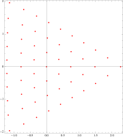
Figure 9. The curvilinear triangle of the branching points for $Sp_{10}(a,\lambda)$.

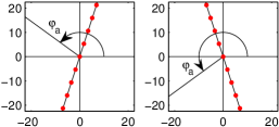
Figure 10. Roots of $Sp_{8}(a,8^{4/3}\beta)$. The left figure shows the situation with $a=500\exp(i\varphi_{a}),\varphi_{a}=4\pi/5$, the right one $a=500\exp(i\varphi_{a}),\varphi_{a}=6\pi/5$. In both cases roots are almost uniformly distributed on the interval $[-\sqrt{a},\sqrt{a}]$.

Proposition 8.

For any given $n$, if $|a|\to\infty$ with $\arg a=\phi$ fixed, then the roots of $Sp_{n}(a,\lambda)$ divided by $n^{4/3}$ will be asymptotically uniformly distributed on the straight segment $[-\sqrt{a},+\sqrt{a}]$, see Figure 10. In particular, if $a$ traverses the circle $Re^{2\pi it},\;t\in[0,1]$ for any sufficiently large $R,$ then the resulting monodromy of roots of $Sp_{n}(R,\lambda)$ (which are all real) is the complete reversing of their order, i.e., the leftmost and the rightmost roots change places, the second from the left and the second from the right change places etc.

Proof of Proposition 8.

Observe that if $a=Ke^{2\pi i\phi}$ with $K$ very large then the polynomial $\widetilde{Sp}_{n}(a,\beta):={n^{-\frac{4(n+1)}{3}}}Sp_{n}(a,\beta n^{4/3})$ is coefficient-wise close to $\widehat{Sp}_{n}(a,\beta)$, where $\widehat{Sp}_{n}(a,\beta)$ is the characteristic polynomial of the tridiagonal matrix

$$\widehat{M}_{n}^{(a)}:=\left(\begin{matrix}0&a/n&0&0&0&\cdots&0\\ n/n&0&2a/n&0&0&\cdots&0\\ 0&(n-1)/n&0&3a/n&0&\cdots&0\\ \vdots&\vdots&\ddots&\ddots&\ddots&\ddots&\vdots\\ 0&0&\cdots&3/n&0&(n-1)a/n&0\\ 0&0&\cdots&0&2/n&0&na/n\\ 0&0&\cdots&0&0&1/n&0\end{matrix}\right).$$ (4.1)

(Observe that the above matrix $\widehat{M}_{n}^{(a)}$ is tridiagonal and not $4$-diagonal as the previous matrices!) To make the situation more transparent, let us consider the sequence of characteristic polynomials of $\frac{1}{\sqrt{a}}\widetilde{M}_{n}^{(a)}$ and of $\frac{1}{\sqrt{a}}\widehat{M}_{n}^{(a)},$ where

$$\widetilde{M}_{n}^{(a)}:=\left(\begin{matrix}0&a/n&2/n&0&0&\cdots&0\\ n/n&0&2a/n&5/n&0&\cdots&0\\ 0&(n-1)/n&0&3a/n&12/n&\cdots&0\\ \vdots&\vdots&\ddots&\ddots&\ddots&\ddots&\vdots\\ 0&0&\cdots&3/n&0&(n-1)a/n&n(n-1)/n\\ 0&0&\cdots&0&2/n&0&na/n\\ 0&0&\cdots&0&0&1/n&0\end{matrix}\right).$$ (4.2)

In other words, we are comparing the roots of $\widetilde{Sp}_{n}(a,\beta)$ divided by $\sqrt{a}$ with that of $\widehat{Sp}_{n}(a,\beta)$ divided by $\sqrt{a}$. The characteristic polynomials of the respective principal minors of $\frac{1}{\sqrt{a}}\widetilde{M}_{n}^{(a)}$ and of $\frac{1}{\sqrt{a}}\widehat{M}_{n}^{(a)}$ satisfy the recurrences:

$$\widetilde{\Delta}_{n}^{(k)}(\gamma)=-\gamma\widetilde{\Delta}_{n}^{(k-1)}(\gamma)-\frac{(k-1)(n-k+2)}{n^{8/3}}\widetilde{\Delta}_{n}^{(k-2)}(\gamma)$$

$$+\frac{(n-k+2)(n-k+3)(k-1)(k-2)}{a^{3/2}n^{4}}\widetilde{\Delta}_{n}^{(k-3)}(\gamma),$$ (4.3)

and

$$\widehat{\Delta}_{n}^{(k)}(\gamma)=-\gamma\widehat{\Delta}_{n}^{(k-1)}(\gamma)-\frac{(k-1)(n-k+2)}{n^{8/3}}\widehat{\Delta}_{n}^{(k-2)}(\gamma),$$ (4.4)

where $\gamma=\beta/\sqrt{a}$ and both recurrences have the standard boundary conditions: $\widetilde{\Delta}_{n}^{(-1)}(\gamma)=\widehat{\Delta}_{n}^{(-1)}(\gamma)=0,\;\widetilde{\Delta}_{n}^{(0)}(\gamma)=\widehat{\Delta}_{n}^{(0)}(\gamma)=1$. As before $\widetilde{Sp}_{n}(a,\beta)=\widetilde{\Delta}_{n}^{(n)}(\gamma)$ and $\widehat{Sp}_{n}(a,\beta)=\widehat{\Delta}_{n}^{(n)}(\gamma)$. Observe now that, for any fixed $n$ and any $\epsilon>0$, one can choose $|a|$ so large that each equation in (4) for $k=1,2,\dots,n$ deviates from the corresponding equation in (4.4) so little that $\widetilde{\Delta}_{n}^{(n)}(\gamma)-\widehat{\Delta}_{n}^{(n)}(\gamma)$ can be made coefficientwise arbitrary small. (This can be done due to the presence of $a^{3/2}$ in the denominator of the third term in (4)).

Now one can easily check by induction that bivariate polynomial $\widehat{Sp}_{n}(a,\beta)$ is quasihomogeneous with weight $1$ for variable $\beta$ and weight $2$ for variable $a$. When $a$ is positive, then $\widehat{Sp}_{n}(a,\beta)$ is a real-rooted polynomial in $\beta$. Since multiplication of $\lambda$ by $e^{\pi it}$ and multiplication of $a$ by $e^{2\pi it}$ multiplies the whole $\widehat{Sp}_{n}(a,\beta)$ by a constant, then for any fixed $a$, the roots of $\widehat{Sp}_{n}(a,\beta)$ with respect to $\beta$ lie on the line through the origin whose slope is half of the slope of $a$. Now consider the roots of $\widehat{Sp}_{n}(a,\beta)$ with respect to $\beta$. Observe that if $a=1$, then the spectrum of (4.1) is $(-1,-1+\frac{2}{n},-1+\frac{4}{n},\dots,1-\frac{4}{n},1-\frac{2}{n},1)$. The same argument as above gives that for any $a\neq 0$, the roots of $\widehat{Sp}_{n}(a,\beta)$ with respect to $\beta$ will be equally spaced on the interval $[-\sqrt{a},\sqrt{a}]$.

Since choosing $|a|$ sufficiently large, we can achieve that all roots of $\widetilde{S}p_{n}^{(n)}(a,\beta)$ lie arbitrarily close to those of $\widehat{S}p_{n}^{(n)}(a,\beta)$, and since the latter roots are equally distributed on the interval $[e^{-2\pi i\phi},e^{-2\pi i\phi}],$ the result follows. ∎

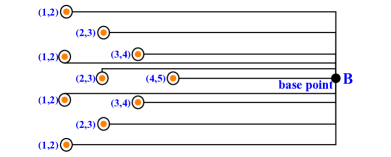
Figure 11. The system of standard paths and the monodromy (transpositions) of the spectrum which they produce for $n=4$.

To describe (our conjecture on) the monodromy of the spectrum, let us introduce a system of standard paths connecting a base point chosen as a sufficiently large positive number with every branching point, see Fig. 11. Based on our numerical experiments, we see that $\Sigma_{n}$ form a triangular shape with points regularly arranged into columns and rows in $\mathbb{C}$. There are $n$ columns (enumerated from left to right) where the $j$-th column consists of $n-j$ branching points with approximately the same real part and there are $n$ rows (enumerated from bottom to top) where the $i$-th row consists of points with approximately the same imaginary part. We denote the branching points $\sigma_{i,j}\in\Sigma_{n}$ where $i=1,\dots,2n-1$ is the row number and $j=1,\dots,n$ is the column number.

Fixing a base point $B$ as a sufficiently large positive number, connect $B$ with every $\sigma_{i,j}$ by a ”vertical hook“ $\mathcal{P}_{i,j}$, i.e., move from $B$ vertically to the imaginary part of $\sigma_{i,j}$, then move horizontally to the left untill you almost hit $\sigma_{i,j}$, then circumgo $\sigma_{i,j}$ counterclockwise along a small circle centered at $\sigma_{i,j}$ and return back to $B$ along the same path. Conjecturally, along such a path one will never hit any other branching points unless $\sigma_{i,j}$ lies on the real axis. In other words, the imaginary parts of all branching points except for the real ones are all distinct. In case when $\sigma_{i,j}$ is real one can slightly deform the suggested path (which is a real interval) in an arbitrary way to move it away from the real axis. The resulting monodromy will (conjecturally) be independent of any such small deformation, see below. Finally we can state our surprisingly simple guess.

Conjecture 4.

For any $\sigma_{i,j}\in\Sigma_{n}$ and any sufficiently large positive base point $B$, the monodromy corresponding to the standard path $\mathcal{P}_{i,j}$ is a simple transposition $(j,j+1)$ of the roots of $Sp_{n}(B,\lambda)$ ordered from left to right. (Recall that by our choice of $B$ all roots of $Sp_{n}(B,\lambda)$ are real and therefore naturally ordered.)

This conjecture has been numerically checked for all $n\leq 10$. Observe that since the system of standard paths gives a basis of the fundamental group $\pi_{1}(\mathbb{C}\setminus\Sigma_{n})$, then knowing the monodromy for the standard paths, one can calculate the monodromy along any loop in $\mathbb{C}\setminus\Sigma_{n}$ based at $B$.

5. Appendix I. Estimates for largest roots of Yablonskii-Vorob’ev polynomials

In this section we present both estimates from above and from below as well as the asymptotic behaviour for roots of maximal modulus of Yablonskii-Vorob’ev polynomials.

The Yablonskii-Vorob’ev polynomials satisfy the differential-difference relation

$$Q_{n+1}(t)=\frac{tQ_{n}(t)^{2}-4(Q_{n}(t)Q_{n}^{{}^{\prime\prime}}(t)-(Q_{n}^{{}^{\prime}}(t))^{2})}{Q_{n-1}(t)}$$ (5.1)

with $Q_{0}(t)=1$ and $Q_{1}(t)=t$. The roots of $Q_{n}$ approximately cover a triangular shape invariant under rotation by $2\pi/3$ whose edges are curves instead of straight lines. The whole pattern is invariant under the dihedral group of symmetries of an equilateral triangle. The roots of maximal modulus lie on a circle with centre the origin. These and other properties are listed in [11].

Our strategy is to connect roots and coefficients of Yablonskii-Vorob’ev polynomials. Similar approach was used in [15]. Our results are sharper and we also derive the asymptotic formula. As the first step we form rational functions

$$\rho_{n}(t)=(\log(Q_{n}(t)))^{{}^{\prime\prime}}-t/4.$$

Another relation between $\rho_{n}$ and $Q_{n}$ is

$$\rho_{n+1}(t)=-Q_{n}(t)Q_{n+2}(t)/(4Q_{n+1}(t)^{2}).$$

From this and from

$$Q_{n}(t)=\prod_{k=1}^{n(n+1)/2}(t-\alpha_{n,k})=\sum_{k=0}^{n(n+1)/2}c_{n,k}t^{k}$$

we see that the Laurent expansion at $\infty$ for $\rho_{n}$ is convergent in $|t|>A_{n+1}$, where $A_{n}:=\max{|\alpha_{n,k}|}_{1\leq k\leq n(n+1)/2}$:

$$\rho_{n}(t)=-\frac{t}{4}-\sum_{j=0}^{\infty}(-1)^{j}\rho_{n,j}t^{-(3j+2)}.$$ (5.2)

A closer inspection reveals that

$$\frac{\rho_{n,j}}{3j+1}=(-1)^{j}s_{n,3j},$$ (5.3)

where $s_{n,j}$ is the sum of $j$th powers of roots of $Q_{n}$, i.e.

$$s_{n,j}=\sum_{k=1}^{n(n+1)/2}\alpha_{n,k}^{j}.$$

The second step is to find the relation between $s_{n,j}$ and $c_{n,k}$, i.e.

$$s_{n,j}=-jc_{n,n(n+1)/2-j}-\sum_{i=1}^{j-1}c_{n,n(n+1)/2-i}s_{n,j-i}.$$ (5.4)

To this end it is suitable to rewrite $Q_{n}(t)$ as

$$Q_{n}(t)=\sum_{k=0}^{[n(n+1)/6]+1}q_{k}(n)t^{(n^{2}+n-6k)/2}.$$ (5.5)

We can find explicit form of $q_{n}$’s:

$$q_{0}(n)= 1$$ (5.6)

$$q_{1}(n)= (n+2)(n+1)n(n-1)/6$$

$$q_{2}(n)= (n+5)(n+3)(n+2)(n+1)n(n-1)(n-2)(n-4)/72$$

$$q_{3}(n)= (n^{4}+2n^{3}-57n^{2}-58n+1120)(n+4)(n+3)(n+2)(n+1)$$

$$n(n-1)(n-2)(n-3)/1296$$

$$\cdots$$

We get $s_{n,j}$ from (5.4). We see that $s_{n,j}\neq 0$ only if $j\equiv 0\,\mathrm{mod}\,3$.

$$s_{n,3}= -(n+2)(n+1)n(n-1)/2$$ (5.7)

$$s_{n,6}= 2(n^{2}+n-5)(n+2)(n+1)n(n-1)$$

$$s_{n,9}= -4(n^{2}+n-7)(3n^{2}+3n-20)(n+2)(n+1)n(n-1)$$

$$s_{n,12}= 8(11n^{6}+33n^{5}-259n^{4}-573n^{3}+2348n^{2}+2640n-7700)$$

$$(n+2)(n+1)n(n-1)$$

$$\cdots$$

Now, we can limit $|A_{n}^{3k}|$. Namely,

$$|A_{n}|\leq\sqrt[3k]{s_{n,3k}},\qquad k=1,2,\ldots.$$ (5.8)

On the other hand, it is clear that $s_{n,3k}$ does not exceed $n(n+1)|A_{n}^{3k}|/2$ and from (5.3) follows (5.9)

$$|A_{n}|\geq\sqrt[3k]{\frac{2\rho_{n,k}}{(3k+1)n(n+1)}}.$$ (5.9)

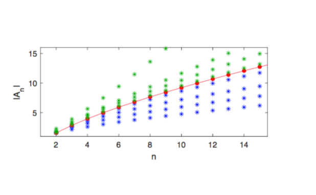
Figure 12. Dependence of $|A_{n}|$ on $n$ (red dots) and the upper (5.8) ($k=1,2,3,10$) (green asterisks) and lower (5.9) ($k=1,2,4,15$) (blue asterisks) limits.

Again,

$$\sqrt[3k]{\frac{2\rho_{n,k}}{(3k+1)n(n+1)}}\geq\sqrt[3(k-1)]{\frac{2\rho_{n,k-1}}{(3k-2)n(n+1)}},$$

so that we have an infinite series of both upper and lower bounds on $|A_{n}|$. This makes possible to find the asymptotic behaviour of $|A_{n}|$ when $n\rightarrow\infty$.

Conserving only the leading term of $s_{n,3k}$ we arrive at a sequence

$$-\frac{n^{4}}{2},2n^{6},-12n^{8},88n^{10},-728n^{12},6528n^{14},-62016n^{16},615296n^{18},-6314880n^{20},\ldots$$

The general form of this sequence is

$$v_{k}=\frac{3(-2)^{k}\Gamma(3k)}{\Gamma(k)\Gamma(2k+3)}n^{2k+2}$$

and

$$\lim_{k\rightarrow\infty}\sqrt[3k]{v_{k}}=\sqrt[3]{-1}\frac{3}{\sqrt[3]{2}}n^{2/3}.$$

Besides, the factor $\sqrt[3]{-1}$ shows the direction in which the three roots of maximal modulus move when $n\rightarrow\infty$.

Numerical results show the rate of convergence to the asymptotic value, cf. table.

$n$	$|A_{n}|$	$3n^{2/3}/\sqrt[3]{2}-|A_{n}|$
10	9.226620959867741	1.82547
20	15.85575092198829	1.68836
30	21.37667838759338	1.61260
40	26.28885026360517	1.56068
50	30.79511630027872	1.52140
60	35.00327495653731	1.48994
70	38.97923077181361	1.46376
80	42.76697737664885	1.44140
90	46.39772099260680	1.42191
100	49.89460772047459	1.40467
110	53.27540358774959	1.38922

6. Appendix II. Complex generalization of the main result of [16]

The main result of this section is Proposition 13 mentioned in § 3 which undoubtedly has independent interest. For the sake of completeness and for the convenience of our readers we include its proof below. Here we adopt the notation used in paper [16] by A. Kuijlaars and W. Van Assche:

$$\lim_{n/N\to t}X_{n,N}=X$$

which denotes that for the doubly indexed sequence it holds that

$$\lim_{j\to\infty}X_{n_{j},N_{j}}=X,$$

for any $\{n_{j}\}_{j\in\mathbb{N}},\ \{N_{j}\}_{j\in\mathbb{N}}\subset\mathbb{N}$ such that $N_{j}\to\infty$ and $n_{j}/N_{j}\to t$, as $j\to\infty$. Additionally, we occasionally add the meaning of the notion of a limit. For example,

$$\operatorname*{w-lim\ }_{n/N\to t}\mu_{n,N}={\mu}$$

expresses the limit of the double indexed sequence of measures $\mu_{n,N}$ converging to $\mu$ in the weak^⋆ topology. Similarly,

$$\operatorname*{s-lim\ }_{n/N\to t}A_{n,N}=A$$

stands for the limit of the double indexed sequence of bounded operators $A_{n,N}$ converging to $A$ strongly.

Recall some well-known facts from the theory of linear operators. First, for any closed operator $T$ on a Banach space, one has

$$\|(T-z)^{-1}\|\geq\frac{1}{\mathop{\mathrm{missing}}{dist}\nolimits(z,\sigma(T))},\quad\forall z\in\rho(T).$$

On the other hand, recall that for a bounded operator $B$ it holds

$$\|(B-z)^{-1}\|\leq\frac{1}{\mathop{\mathrm{missing}}{dist}\nolimits(z,D_{\|B\|})},\quad\forall z,\;|z|>\|B\|,$$

where $D_{\|B\|}=\{z\in\mathbb{C}\mid|z|\leq\|B\|\}$. Let us remark that $\sigma(B)\subset D_{\|B\|}$.

Let $\{a_{n}\}_{n\geq 1},\{b_{n}\}_{n\geq 0}\subset\mathbb{C}$ and $a_{n}\neq 0$, $\forall n\geq 1$. Further $J_{n}$ denotes the $(n+1)\times(n+1)$ Jacobi matrix of the form

$$J_{n}=\begin{pmatrix}b_{0}&a_{1}\\ a_{1}&b_{1}&a_{2}\\ &a_{2}&b_{2}&a_{3}\\ &&\ddots&\ddots&\ddots\\ &&&a_{n-1}&b_{n-1}&a_{n}\\ &&&&a_{n}&b_{n}\end{pmatrix}.$$

Recall also that the polynomial sequence $\{p_{n}\}_{n\geq 0}$ determined by recurrence

$$a_{n}p_{n-1}(x)+b_{n}p_{n}(x)+a_{n+1}p_{n+1}(x)=xp_{n}(x),\quad n\geq 0,$$

and initial conditions $p_{-1}=0$ and $p_{0}=1$, is related with $J_{n}$ by formula

$$p_{n}(x)=\left(\prod_{k=1}^{n}\frac{1}{a_{k}}\right)\det\left(x-J_{n-1}\right),\quad n\geq 1.$$

Lemma 9.

[16, Lem. 2.2] Let $\|J_{n}\|\leq M$, then

$$\left|\frac{p_{n}(z)}{a_{n+1}p_{n+1}(z)}\right|\leq\frac{1}{\mathop{\mathrm{missing}}{dist}\nolimits(z,D_{M})}=\frac{1}{|z|-M},\quad\forall z\in\mathbb{C},|z|>M.$$

On the other hand, one has

$$\left|\frac{p_{n}(z)}{a_{n+1}p_{n+1}(z)}\right|\geq\frac{1}{2|z|}\quad\forall z\in\mathbb{C},|z|>3M.$$

Proof.

By simple linear algebra,

$$\frac{p_{n}(z)}{a_{n+1}p_{n+1}(z)}=\frac{\det\left(z-J_{n-1}\right)}{\det\left(z-J_{n}\right)}=\langle e_{n},(z-J_{n})^{-1}e_{n}\rangle$$

(note that $e_{n}$ stands for the $(n+1)$-th vector of the standard basis of $\mathbb{C}^{n+1}$). Consequently,

$$\left|\frac{p_{n}(z)}{a_{n+1}p_{n+1}(z)}\right|=|\langle e_{n},(z-J_{n})^{-1}e_{n}\rangle|\leq\|(z-J_{n})^{-1}\|\leq\frac{1}{\mathop{\mathrm{missing}}{dist}\nolimits(z,D_{\|J_{n}\|})}\leq\frac{1}{\mathop{\mathrm{missing}}{dist}\nolimits(z,D_{M})},$$

whenever $|z|>M$.

One the other hand,

$$|\langle e_{n},(z-J_{n})^{-1}e_{n}\rangle|=\frac{1}{|z|}\left|1+\langle e_{n},\sum_{k=1}^{\infty}z^{-k}J_{n}^{k}e_{n}\rangle\right|\geq\frac{1}{|z|}\left(1-\frac{\|J_{n}\|}{|z|-\|J_{n}\|}\right)\geq\frac{1}{2|z|},$$

whenever $|z|\geq 3M$. ∎

Observe that if $R_{n}\in\mathbb{C}^{n+1,n+1}$ is the permutation matrix determined by equations $R_{n}e_{k}=e_{n-k}$, $\forall k\in\{0,1,\dots,n\}$, then

$$R_{n}J_{n}R_{n}=\begin{pmatrix}b_{n}&a_{n}\\ a_{n}&b_{n-1}&a_{n-1}\\ &a_{n-1}&b_{n-2}&a_{n-2}\\ &&\ddots&\ddots&\ddots\\ &&&a_{2}&b_{1}&a_{1}\\ &&&&a_{1}&b_{0}\end{pmatrix},$$

$\det(J_{n}-z)=\det(R_{n}J_{n}R_{n}-z)$, and

$$\langle e_{n},(J_{n}-z)^{-1}e_{n}\rangle=\langle e_{0},(R_{n}J_{n}R_{n}-z)^{-1}e_{0}\rangle,\quad\forall z\in\rho(J_{n}).$$

If convenient, we identify matrix $R_{n}$ with the operator $R_{n}\oplus 0$ acting on $\ell^{2}(\mathbb{N}_{0})$

In what follows, $\{a_{n,N}\mid n,N\in\mathbb{N}\}\subset\mathbb{C}$, $\{b_{n,N}\mid n\in\mathbb{N}_{0},\;N\in\mathbb{N}\}\subset\mathbb{C}$, and

$$J(N)=\begin{pmatrix}b_{0,N}&a_{1,N}\\ a_{1,N}&b_{1,N}&a_{2,N}\\ &a_{2,N}&b_{2,N}&a_{3,N}\\ &&\ddots&\ddots&\ddots\end{pmatrix}$$

stands for the semi-infinite (complex) Jacobi matrix. Finally, $P_{n}\in\mathcal{B}(\ell^{2}(\mathbb{N}_{0}))$ denotes the orthogonal projection on $\mathop{\mathrm{missing}}{span}\nolimits\{e_{0},\dots,e_{n}\}$.

Proposition 10.

Let

$$\lim_{n/N\to t}a_{n,N}=A\quad\mbox{ and }\lim_{n/N\to t}b_{n,N}=B.$$ (6.1)

Further assume that there exists $\epsilon>0$ such that

$$\sup\{\|P_{n}J(N)P_{n}\|\mid|n/N-t|<\epsilon\}<\infty.$$ (6.2)

Then

$$\operatorname*{s-lim\ }_{n/N\to t}R_{n}J(N)R_{n}=J(A,B)$$

where $J(A,B)\in\mathcal{B}(\ell^{2}(\mathbb{N}_{0}))$ stands for the Jacobi matrix with constant diagonal $B$ and constant off-diagonal $A$.

Proof.

Recall an easily verifiable statement: Let $\mathcal{X}$ be a Banach space, $B\in\mathcal{B}(\mathcal{X})$ and $B_{n}$ a uniformly bounded sequence of operators acting on $\mathcal{X}$. If $B_{n}\varphi\to B\varphi$, as $n\to\infty$, for all $\varphi$ from a dense subset of $\mathcal{X}$, then $\operatorname*{s-lim\ }_{\!n\to\infty}B_{n}=B$.

Take arbitrary $\{n_{j}\},\{N_{j}\}\subset\mathbb{N}$, $N_{j}\to\infty$ and $n_{j}/N_{j}\to t$, for $j\to\infty$. Let us denote temporarily $\hat{J}_{j}=R_{n_{j}}J(N_{j})R_{n_{j}}$ Assumption (6.2) guarantees the existence of $j_{0}\in\mathbb{N}$ such that

$$\sup_{j\geq j_{0}}\|P_{n_{j}}J(N_{j})P_{n_{j}}\|=\sup_{j\geq j_{0}}\|\hat{J}_{j}\|<\infty.$$

Hence, taking into account the above statement, it suffices to verify that

$$\lim_{j\to\infty}\hat{J}_{j}e_{n}=J(A,B)e_{n},\quad\forall n\in\mathbb{N}_{0}.$$

Take $n\in\mathbb{N}_{0}$ and $j>n$, then

$$\|\hat{J}_{j}e_{n}-J(A,B)e_{n}\|^{2}=|a_{n_{j}-n+1,N_{j}}-A|^{2}+|b_{n_{j}-n,N_{j}}-B|^{2}+|a_{n_{j}-n,N_{j}}-A|^{2}\to 0,$$

for $j\to\infty$, by assumption (6.1). If $n=0$, set $a_{n_{j}+1,N_{j}}=0$ in the above equation. All in all, the claim is verified. ∎

It is again quite easy to see that for any $B_{n},B\in\mathcal{B}(\mathcal{X})$ such that $\sup_{n}\|B_{n}\|\leq M$ and $\operatorname*{s-lim\ }_{\!n\to\infty}B_{n}=B$, one has

$$\operatorname*{s-lim\ }_{n\to\infty}(B_{n}-z)^{-1}=(B-z)^{-1},\quad\forall z\notin D_{M}$$

and the convergence is local uniform in $z$. Indeed, since

$$(B-z)^{-1}-(B_{n}-z)^{-1}=(B_{n}-z)^{-1}(B_{n}-B)(B-z)^{-1}$$

one obtains

$$\|(B-z)^{-1}\varphi-(B_{n}-z)^{-1}\varphi\|\leq\frac{1}{|z|-M}\|(B_{n}-B)(B-z)^{-1}\varphi\|,$$

from which the strong convergence of resolvents follows. The local uniformness follows, for example, from the Mantel’s theorem.

The next statement is in fact a corollary of Proposition 10, however, it is also a complex generalization of [16, Thm. 2.1]. Therefore we formulate it as a proposition.

Proposition 11.

[16, Thm. 2.1] Let the assumptions (6.1) and (6.2) hold. Denote the value of the supremum in (6.2) by $M$. Then

$$\lim_{n/N\to t}\langle e_{n},\left(z-P_{n}J(N)P_{n}\right)^{-1}e_{n}\rangle=\frac{2}{z-B+\sqrt{(z-B)^{2}-4A^{2}}}$$

locally uniformly in $\mathbb{C}\setminus D_{M}$.

Remark 10.

Note that by (6.1),

$$M=\sup\{\|P_{n}J(N)P_{n}\|\mid|n/N-t|<\epsilon\}\geq|B|+2|A|.$$

Proof.

It follows from Proposition 10 that

$$\operatorname*{s-lim\ }_{n/N\to t}\left(z-R_{n}J(N)R_{n}\right)^{-1}=\left(z-J(A,B)\right)^{-1}$$

locally uniformly in $z\notin D_{M}$. Hence,

$$\lim_{n/N\to t}\langle e_{n},\left(z-P_{n}J(N)P_{n}\right)^{-1}e_{n}\rangle =\lim_{n/N\to t}\langle e_{0},\left(z-R_{n}J(N)R_{n}\right)^{-1}e_{0}\rangle$$

$$=\langle e_{0},\left(z-J(A,B)\right)^{-1}e_{0}\rangle$$

locally uniformly in $z\notin D_{M}$. It is a standard result that

$$\langle e_{0},\left(z-J(A,B)\right)^{-1}e_{0}\rangle=\frac{2}{z-B+\sqrt{(z-B)^{2}-4A^{2}}},$$

for all $z\notin[B-2A,B+2A]$ (a line segment in $\mathbb{C}$). To verify that one can show that

$$\operatorname*{s-lim\ }_{n\to\infty}P_{n}J(A,B)P_{n}=J(A,B)$$

together with the formula

$$\langle e_{0},\left(z-J_{n}(A,B)\right)^{-1}e_{0}\rangle=\frac{U_{n}\left(\frac{z-B}{2A}\right)}{A\ U_{n+1}\left(\frac{z-B}{2A}\right)},\quad\forall z\notin[B-2A,B+2A]$$

where $J_{n}(A,B)$ stands for the $(n+1)\times(n+1)$ truncation of $J(A,B)$, i.e., $J(A,B)=J_{n}(A,B)\oplus 0$, and

$$U_{n}(x)=\frac{\left(x+\sqrt{x^{2}-1}\right)^{n+1}-\left(x-\sqrt{x^{2}-1}\right)^{n+1}}{2\sqrt{x^{2}-1}}$$

are Chebyshev polynomials of the second kind. ∎

Recall that the main result of paper [16] in Theorem 1.4. which claims the following.

Theorem 12.

[16, Thm. 1.4] If $\{a_{n,N}\mid n,N\in\mathbb{N}\}\subset{\mathbb{R}}_{+}$, $\{b_{n,N}\mid n\in\mathbb{N}_{0},\;N\in\mathbb{N}\}\subset{\mathbb{R}}$ and $\{p_{n,N}\mid n\in\mathbb{N}_{0},\;N\in\mathbb{N}\}$ associated family of orthonormal polynomials. Further let non-negative $a\in C({\mathbb{R}}_{+})$ and real $b\in C({\mathbb{R}}_{+})$ be given, such that

$$\lim_{n/N\to t}a_{n,N}=a(t)\quad\mbox{ and }\lim_{n/N\to t}b_{n,N}=b(t),$$

for all $t>0$. Then for the family of $\{\nu_{n,N}\mid n\in\mathbb{N}_{0},\;N\in\mathbb{N}\}$ of root-counting measures of polynomials $\{p_{n,N}\mid n\in\mathbb{N}_{0},\;N\in\mathbb{N}\}$, one has

$$\operatorname*{w-lim\ }_{n/N\to t}\nu_{n,N}=\frac{1}{t}\int_{0}^{t}\omega_{[b(s)-2a(s),b(s)+2a(s)]}{\rm d}s$$

where $\omega_{[\alpha,\beta]}$ is absolutely continuous measure supported on $[\alpha,\beta]$ with density

$$\frac{{\rm d}\omega_{[\alpha,\beta]}}{{\rm d}t}=\frac{1}{\pi\sqrt{(\beta-t)(t-\alpha)}},$$

if $\alpha<\beta$. If $\alpha=\beta$, $\omega_{[\alpha,\beta]}=\delta_{\{\alpha\}}$.

For $t>0$, let us denote

$$\sigma(t)=\frac{1}{t}\int_{0}^{t}\omega_{[b(s)-2a(s),b(s)+2a(s)]}{\rm d}s.$$

In the proof of Theorem 12, authors prove that

$$\lim_{n/N\to t}U^{\nu_{n,N}}(z)=U^{\sigma(t)}(z)$$ (6.3)

locally uniformly in certain neighborhood of complex $\infty$ (i.e., for $|z|>M$), where $U^{\mu}$ denotes the logarithmic potential of the (compactly supported) Borel measure $\mu$. Under the assumptions of Theorem 12, supports of all measures $\nu_{n,N}$, for all $n,N$ such that $n/N$ is close to $t$, are included in a real interval $[-M,M]$. This implies that the limit relation (6.3) holds true for all $z\notin[-M,M]$ and hence for almost all $z\in\mathbb{C}$ (w.r.t. the Lebesgue measure). Under these conditions one can show (following standard methods of Potential Theory - Widom’s lemma) the weak convergence

$$\operatorname*{w-lim\ }_{n/N\to t}\nu_{n,N}=\sigma(t).$$ (6.4)

However, in the general case of complex sequences $a_{n,N}$ and $b_{n,N}$, one can get only the relation (6.3) outside a ball, $|z|>M$, and not for almost all $z\in\mathbb{C}$. This however does not imply the weak convergence (6.4). To our best knowledge nor the existence of the weak limit is guaranteed (only a subsequence, by Helly’s theorem). Thus, one can not expect the validity of Theorem 12 in the complex setting. However, one can get at least the following.

Proposition 13.

Let $a\in C([0,\infty))$ and $b\in C([0,\infty))$ be complex-valued functions and

$$\lim_{n/N\to t}a_{n,N}=a(t)\quad\mbox{ and }\lim_{n/N\to t}b_{n,N}=b(t),$$

for all $t>0$. Then if the weak limit of root-counting measures

$$\nu=\operatorname*{w-lim\ }_{n/N\to t}\nu_{n,N}$$

exists, then $\nu$ and $\sigma(t)$ are equipotential measures, i.e., their logarithmic potentials coincide outside the union of their supports.

Remark 11.

Note the functions $a$ and $b$ are assumed to be continuous in $0$ (from the right). This additional condition simplifies the proof considerably and we do not aim here to achieve a full generality.

Proof.

Note that coefficients $a_{n,N}$ and $b_{n,N}$ are uniformly bounded if $n/N$ is restricted to a compact subsets of $[0,\infty)$, as it follows from the assumptions. Take $t>0$ and $0<\epsilon<t$, then

$$\sup\{|b_{n,N}|\mid|n/N-t|\leq\epsilon\}+2\sup\{|a_{n,N}|\mid|n/N-t|\leq\epsilon\}<\infty.$$

Denote by $J_{n}(N)$ the $(n+1)\times(n+1)$ truncation of $J(N)$. Consequently, condition (6.2) is fulfilled and let us denote the uniform bound of operators $J_{n}(N)$, for $|n/N-t|\leq\epsilon$, by $M$.

The following part proceeds analogously as the proof of [16, Thm. 1.4]. Since

$$\frac{\det\left(z-J_{n-1}(N)\right)}{\det\left(z-J_{n}(N)\right)}=\langle e_{n},(z-J_{n}(N))^{-1}e_{n}\rangle,$$

one has

$$\det\left(z-J_{n}(N)\right)=\prod_{k=0}^{n}\frac{1}{\langle e_{k},(z-J_{k}(N))^{-1}e_{k}\rangle},\quad|z|>M.$$

Thus,

$$U^{\nu_{n,N}}(z)=\frac{1}{n+1}\log\left|\det\left(z-J_{n}(N)\right)\right|=-\frac{1}{n+1}\sum_{k=0}^{n}\log\left|\langle e_{k},(z-J_{k}(N))^{-1}e_{k}\rangle\right|,$$

or equivalently

$$U^{\nu_{n,N}}(z)=-\int_{0}^{1}\log\left|\langle e_{[ns]},(z-J_{[ns]}(N))^{-1}e_{[ns]}\rangle\right|{\rm d}s,\quad|z|>M.$$

As $n/N\to t$, one has $[sn]/N\to st$. Hence, by Proposition 11,

$$\lim_{n/N\to t}\langle e_{[ns]},(z-J_{[ns]}(N))^{-1}e_{[ns]}\rangle=\frac{2}{z-b(st)+\sqrt{(z-b(st))^{2}-4a(st)^{2}}}.$$

Further, by Lemma 9, one has

$$\frac{1}{2|z|}\leq\left|\langle e_{[ns]},(z-J_{[ns]}(N))^{-1}e_{[ns]}\rangle\right|\leq\frac{1}{|z|-M},$$

for $|z|>3M$. Consequently, the Lebesgue’s dominated convergence theorem applies and we get

$$\lim_{n/N\to t}U^{\nu_{n,N}}(z) =\int_{0}^{1}\log\left|\frac{z-b(st)}{2}+\sqrt{\left(\frac{z-b(st)}{2}\right)^{2}-a(st)^{2}}\right|{\rm d}s$$

$$=\frac{1}{t}\int_{0}^{t}\log\left|\frac{z-b(s)}{2}+\sqrt{\left(\frac{z-b(s)}{2}\right)^{2}-a(s)^{2}}\right|{\rm d}s$$

for $|z|>3M$. The function in the last integral is known to coincide with the logarithmic potential of $\omega_{[b(s)-2a(s),b(s)+2a(s)]}$ at $z$. All in all, we obtained

$$U^{\nu}(z)=\frac{1}{t}\int_{0}^{t}U^{\omega_{[b(s)-2a(s),b(s)+2a(s)]}}(z){\rm d}s=U^{\sigma(t)}(z),$$

for $|z|>3M$. By the harmonicity of logarithmic potentials $U^{\mu}$ outsides the support $\mu$ and Identity principle for harmonic functions the last equality can be extended to all $z\notin(\mathop{\mathrm{missing}}{supp}\nolimits\nu\cup\mathop{\mathrm{missing}}{supp}\nolimits\sigma(t))$. ∎

References

- [1] C. Bender and S. Boettcher, Quasi-exactly solvable quartic potential, J. Phys. A 31 (1998), no. 14, L273-L277.
- [2] S. Beraha, J. Kahane, N. J. Weiss, Limits of zeros of recursively defined families of polynomials, in “Studies in Foundations and Combinatorics”, pp. 213–232, Advances in Mathematics Supplementary Studies Vol. 1, ed. G.-C. Rota, Academic Press, New York, 1978.
- [3] M. Bertola, T. Bothner, Zeros of large degree Vorob’ev-Yablonski polynomials via a Hankel determinant identity. Int. Math. Res. Not. IMRN 2015, no. 19, 9330–9399.
- [4] J. Borcea, R. Bøgvad, and B. Shapiro, On rational approximation of algebraic functions, Adv. Math. vol 204, issue 2 (2006) 448–480.
- [5] J. Borcea, R. Bøgvad and B. Shapiro, Homogenized spectral pencils for exactly solvable operators: asymptotics of polynomial eigenfunctions, Publ. RIMS, vol 45 (2009) 525–568.
- [6] R. Bøgvad, B. Shapiro, On motherbody measures with algebraic Cauchy transform, Enseign. Math. 62 (2016), no. 1-2, 117–142.
- [7] A. Bourget, T.McMillen, On the distribution and interlacing of the zeros of Stieltjes polynomials, Proc. AMS 138 (2010), 3267–3275.
- [8] A. Bourget, T.McMillen, A. Vargas, Interlacing and nonorthogonality of spectral polynomials for the Lamé operator, Proc. AMS 137 (2009), 1699–1710.
- [9] R. J. Buckingham, P. D. Miller, Large-degree asymptotics of rational Painlevé II functions: noncritical behaviour. Nonlinearity 27 (2014), no. 10, 2489–2578.
- [10] R. J. Buckingham, P. D. Miller, Large-degree asymptotics of rational Painlevé II functions: critical behaviour. Nonlinearity 28 (2015), no. 6, 1539–1596.
- [11] P. A. Clarkson, E. L. Mansfield, The second Painlevé equation, its hierarchy and associated special polynomials, Nonlinearity 16 (2003), R1–R26.
- [12] E. Coussement, J. Coussement and W.Van Assche, Asymptotic zero distribution for a class of multiple orthogonal polynomials, Trans. Amer. Math. Soc. 360 (2008), 5571-5588.
- [13] A. Eremenko, A. Gabrielov, Quasi-exactly solvable quartic: elementary integrals and asymptotics, J. Phys. A: Math. Theor. 44 (2011) 312001.
- [14] S. Fisk, Polynomials, roots, and interlacing, arXiv:math/0612833.
- [15] Y. Kametaka, On Poles of the Rational Solution of the Toda Equation of Painlevé-II Type, Proc. Japan Acad. Ser A, 59(A) (1983) 358–360.
- [16] A. B. J. Kuijlaars, W. Van Assche, The asymptotic zero distribution of orthogonal polynomials with varying recurrence coefficients, J. Approx. Theory 99 (1999), 167–197.
- [17] D. Masoero, Poles of integrale tritronquée and anharmonic oscillators. A WKB approach. J. Phys. A: Math. Theor., 43(9), 5201, 2010.
- [18] D. Masoero, V. De Benedetti, Poles of integrale tritronquée and anharmonic oscillators. Asymptotic localization from WKB analysis. Nonlinearity 23:2501, 2010.
- [19] E. Mukhin, V. Tarasov, On conjectures of A. Eremenko and A. Gabrielov for quasi-exactly solvable quartic. Lett. Math. Phys. 103 (2013), no. 6, 653–663.
- [20] N. Nilsson, Some growth and ramification properties of certain integrals on algebraic manifold,. Ark. Mat. 5 1965 463–476 (1965).
- [21] M. Petkovek, H. Zakrajek, Pascal-like determinants are recursive, Adv. Appl. Math., 33 (2004), 431–450.
- [22] B. Shapiro, and M. Tater, Asymptotics of spectral polynomials, Acta Polytechnica vol 47(2-3) (2007) 32–35.
- [23] B. Shapiro, and M. Tater, On spectral polynomials of the Heun equation. I, JAT, 162 (2010) 766–781.
- [24] K. Shin, Eigenvalues of PT-symmetric oscillators with polynomial potentials, J. Phys. A 38 (2005), no. 27, 6147–6166.
- [25] K. Strebel, Quadratic differentials, Ergebnisse der Mathematik und ihrer Grenzgebiete, 5, Springer-Verlag, Berlin, (1984), xii+184 pp.
- [26] B. Shapiro, K. Takemura, and M. Tater, On spectral polynomials of the Heun equation. II, Comm. Math. Phys. 311(2) (2012), 277–300.
- [27] M. Taneda, Remarks on the Yablonskii-Vorob’ev polynomials, Nagoya Math. J., 159 (2000), 87–111.
- [28] A. Vorob’ev, On rational solutions of the second Painlevé equations, Diff. Eqns (1) (1965), 58–59 (in Russian).
- [29] A. Yablonskii, On rational solutions of the second Painlevé equation, Vesti Akad. Navuk. BSSR Ser. Fiz. Tkh. Nauk. 3 (1959), 30–35 (in Russian).