Absorption of waves by large scale winds in stratified turbulence

Abstract

The atmosphere is a nonlinear stratified fluid in which internal gravity waves are present. These waves interact with the flow, resulting in wave turbulence that displays important differences with the turbulence observed in isotropic and homogeneous flows. We study numerically the role of these waves and their interaction with the large scale flow, consisting of vertically sheared horizontal winds. We calculate their space and time resolved energy spectrum (a four-dimensional spectrum), and show that most of the energy is concentrated along a dispersion relation that is Doppler shifted by the horizontal winds. We also observe that when uniform winds are let to develop in each horizontal layer of the flow, waves whose phase velocity is equal to the horizontal wind speed have negligible energy. This indicates a nonlocal transfer of their energy to the mean flow. Both phenomena, the Doppler shift and the absorption of waves traveling with the wind speed, are not accounted for in current theories of stratified wave turbulence.

I Introduction

Turbulent flows are often pictured as highly disorganized, with energy being transferred from large scale motions to small scale eddies. But in some cases the opposite can happen. In 1967 Kraichnan Kraichnan and Montgomery (1980) developed the theory of the inverse energy cascade, in which nonlinearities transfer energy towards larger structures in a self-organization process. The theory had a huge impact in oceanography and meteorology, and in the basic physical understanding of turbulence. However, an inverse cascade is not the only possible mechanism by which energy can be transferred from small to large scales, and in some flows other mechanisms can result in the generation of large scale flows.

An important example is given by stratified flows. Stratification plays a key role in the dynamics of the oceans and the atmosphere. As an example, internal gravity waves arising from it are responsible for transfer of momentum between different regions of the atmosphere Hines (1972), and for transport in the oceans Ledwell et al. (2000); Gargett et al. (2004). Much effort has been put in characterizing internal gravity waves and their relation with geophysical flows Riley and Lelong (2000); Staquet and Sommeria (2002); Ivey et al. (2008).

Several observational studies suggest there is a coupling between the mean (or large-scale) flow and internal gravity waves Finnigan et al. (1984); Dohan and Sutherland (2003); Xing and Davies (2005). As a result, various models for the interaction between a wave field and a mean background flow have been put forward Grimshaw (1972, 1975); Hines (1991). These models, which were mainly developed in the context of atmospheric sciences and oceanography, predict that the dispersion relation of the waves is Doppler shifted by the background flow. Furthermore, they also describe an instability by which waves whose horizontal phase velocity matches that of the horizontal wind speed on a given layer of the fluid, are absorbed by the background flow. This is the so-called critical layer (CL) instability. A fraction of the energy in the waves is then transferred towards the mean flow, and the rest is dissipated. However, most CL models are either linear or perturbative, have the large scale shear externally imposed, lack nonlinear coupling between the waves themselves as well as with small-scale eddies, and cannot fully describe the nonlinear dynamics of a turbulent geophysical flow. Important observational studies of the atmosphere Gossard et al. (1970) and the ocean Kunze et al. (1990), and laboratory experiments Thorpe (1981); Koop and McGee (1986) focusing on the properties of single waves passing through, show Doppler shift and indications of CL instability, although they lack the presence of a fully developed turbulent superposition of waves. In the same spirit, numerical studies of Doppler shift and CL instability Grimshaw (1975); Hines (1991); Winters and D’Asaro (1994); Broutman et al. (1997) that solve nonlinear atmospheric models, focus on single wave packets interacting with a background flow which is externally imposed, and do not take into account the turbulent nature of geophysical flows nor the nonlinear interaction between the internal gravity waves themselves and with the eddies present in the flow (see however Winters and D’Asaro (1994), where the full nonlinear equations are solved, although a single wavepacket and background flow are imposed). This can be understood as identifying waves in a smooth flow can be done by observing the time evolution of the system, while extraction of the waves in a disordered background requires space and time information.

On the other hand, fluid dynamics studies, both theoretically and numerically (see, e.g., Billant and Chomaz (2001); Waite and Bartello (2006); Brethouwer et al. (2007); Lindborg and Brethouwer (2007)), focused mainly on the fully nonlinear aspect of stratified turbulence, on how energy is distributed among scales, and on the development of anisotropy and of flat “pancake” structures in the flow. These studies remark that the interaction between waves and eddies is of fundamental importance in stratified turbulence, but have neglected the effects of Doppler shifts or CL instability. An important topic which is subject to an active debate is the existence of an inverse cascade in purely stratified flows. As already mentioned, an inverse cascade is a self-similar process by which energy is transferred nonlinearly from small scales to larger scales, so energy gets accumulated in structures with larger correlation length than that of the injection mechanism. Inverse cascades have been extensively studied in two dimensional turbulence Kraichnan and Montgomery (1980), and have also been observed in rotating turbulence (including rotating stratified turbulence) Bartello (1995); Pouquet and Marino (2013); Yarom and Sharon (2014). But results for purely stratified turbulence are unclear. It is known that stratified flows can generate large-scale vertically sheared horizontal winds (VSHW) Smith and Waleffe (2002), although the mechanism involved is not entirely understood. While evidence of energy flow toward large scales has been reported Marino et al. (2013, 2014), several authors have argued that an inverse cascade is not possible Waite and Bartello (2006); Herbert et al. (2014) based on statistical mechanical arguments.

Recently, weak turbulence theory Nazarenko (2011); Lvov and Tabak (2001) has also been used to study stratified turbulence, although only considering the coupling between the waves and not with the eddies. While this theory can give information on the formation of the nonlinear energy cascade, it cannot characterize interactions of the wave field with a mean flow. Some extensions that consider nonlocal interactions and the development of zonal flows have been proposed to address this, and are specially relevant in the context of quasi-geostrophic turbulence James (1987), and plasma turbulence in tokamaks Diamond et al. (2005); Connaughton et al. (2011) to explain the development of large-scale flows.

In this article, we identify a mechanism working within a stably stratified turbulent flow that couples the wave field with the large-scale VSHW, thus gaining a better understanding of the role of waves and the generation of large structures in turbulent flows. We obtain for the first time the four-dimensional space and time resolved energy spectra, allowing us to uniquely identify the wave components of the total flow and to study their dynamics. We show that waves are Doppler shifted by the VSHW, and that while a direct nonlinear energy cascade is present, energy can also be transferred nonlocally from the small-scale waves to the large-scale flow though CL instabilities. Finally, we also show that the energy spread created by the Doppler shift is not uniform, a fact that results from the turbulent nature of the dynamically evolving large-scale flow.

II Stably stratified flows

In this section we present the equations we solve numerically that describe a stably stratified flow, introduce characteristic time scales, and give a brief introduction to the linear theory of gravity waves in the presence of background shear.

II.1 The Boussinesq equations

We consider the Boussinesq equations describing an incompressible stratified flow,

$$\partial_{t}\mathbf{u}+{\bf u}\cdot{\bf\nabla}{\bf u} = -{\bf\nabla}p-N\theta\hat{z}+\nu\nabla^{2}{\bf u}+{\bf F},$$ (1)

$$\partial_{t}\theta+{\bf u}\cdot{\bf\nabla}\theta = Nu_{z}+\kappa\nabla^{2}\theta,$$ (2)

where ${\bf u}$ is the velocity field (with ${\bf\nabla}\cdot{\bf u}=0$), $\theta$ is the potential temperature fluctuations, $p$ is the pressure normalized by the mean fluid density, $\nu$ is the kinematic viscosity, $\kappa$ is the thermal diffusivity, $N$ is the Brunt-Väisälä frequency (associated with the vertical background stratification), and ${\bf F}$ is an external mechanical forcing.

In the absence of a background flow, of forcing (${\bf F}=0$), and of viscosity and diffusion ($\nu=\kappa=0$), Eqs. (1) and (2) have as exact nonlinear solutions Majda (2003) internal gravity waves with dispersion relation

$$\omega_{0}=N\frac{k_{\perp}}{k}.$$ (3)

Here $k_{\perp}=(k^{2}_{x}+k^{2}_{y})^{1/2}$ is the wavenumber perpendicular to gravity. Gravity acts along the $\hat{z}$ axis, with associated wavenumber $k_{\parallel}=k_{z}$ such that $k=(k^{2}_{\perp}+k^{2}_{\parallel})^{1/2}$.

II.2 Characteristic timescales

The important characteristic timescales that come into play in this system are the wave period $\tau_{\omega}$, and the nonlinear turnover time $\tau_{NL}$. The wave period is simply given by $\tau_{\omega}\propto 1/\omega_{0}$. The nonlinear turnover time is the time taken by an eddie at a certain scale to transfer its energy through nonlinear interactions to smaller scale eddies locally in wavenumber space. From dimensional analysis, this timescale can be estimated as

$$\tau_{NL}\propto\frac{\ell}{u_{\ell}}\propto\frac{1}{k\sqrt{kE(k)}},$$ (4)

where $\ell\propto 1/k$ is a lengthscale in the inertial range, $u_{\ell}$ is the characteristic velocity of eddies at scale $\ell$, and $E(k)$ is the energy spectrum. If the energy spectrum in stratified turbulence follows a power law $E(k)\propto k^{-3}$ (see, e.g., Billant and Chomaz (2001)), then it is easy to show that the turnover time is independent of the scale, and becomes $\tau_{NL}\propto L/u_{\textrm{rms}}$ at all scales.

II.3 Gravity waves in a background flow

In the presence of a background horizontal flow ${\bf U}(z)$, the frequency measured by an observer is shifted by the Doppler effect, resulting in a frequency

$$\omega=\omega_{0}+{\bf U}\cdot{\bf k}_{\perp}.$$ (5)

Considering for simplicity the unidirectional case with ${\bf U}=U(z)\hat{x}$, and substituting ${\bf u}={\bf U}+{\bf u^{\prime}}$ in Eqs. (1) and (2) with ${\bf u^{\prime}}=w(z)e^{ik_{\perp}(x-ct)}\hat{z}$ a planar internal gravity wave propagating in $\hat{x}$ with phase velocity $c=\omega/k$, we obtain after linearization an equation for the vertical velocity amplitude Booker and Bretherton (1967)

$$\frac{\partial^{2}w}{\partial z^{2}}+\left[\frac{N^{2}}{(U-c)^{2}}-\frac{d^{2}U/dz^{2}}{U-c}-k_{\perp}^{2}\right]w=0.$$ (6)

This equation has a singularity when $c=U(z)$, which is associated with the existence of a CL in which the Reynolds stress tensor has a discontinuity Booker and Bretherton (1967). As a result, a wave traveling through the fluid an approaching the layer with $c=U(z)$ develops faster and faster fluctuations in its vertical velocity amplitude, becomes unstable, and finally degenerates into turbulence, transferring a fraction of its energy to the background flow, while the rest is dissipated. These latter processes cannot be properly described by the linear theory. In practice, the instability only occurs if the Richardson number, $\textrm{Ri}=N^{2}/(\partial_{z}U)^{2}$, is greater than $1/4$ Booker and Bretherton (1967).

Going beyond the linear regime, the detailed numerical study in Winters and D’Asaro (1994) considers the energy balance when a wave packet crosses a CL. The authors were able to quantify that more than a third of the energy in the waves is nonlocally transferred to the mean background flow, while the rest of the energy in the waves is transferred towards the small scale turbulence where it is finally dissipated.

III Numerical simulations

Direct numerical simulations of Eqs. (1) and (2) were performed in a cubic periodic box using the parallel code GHOST Gómez et al. (2005a, b); Mininni et al. (2011) that uses a pseudospectral method to estimate spatial derivatives, and evolves the system in time using a second-order Runge-Kutta method. Two forcing functions were used: Taylor-Green forcing with ${\bf F}=f_{0}(\sin x\cos y\cos z\,\hat{x}-\cos x\sin y\cos\,\hat{z})$, and a randomly generated isotropic three-dimensional forcing acting at $k=1$. As we will consider frequency spectra, in both cases the forcing was kept constant in time to prevent exciting spurious timescales in the system, and to prevent disrupting the development of VSHW.

A Taylor-Green flow excites two-dimensional motions and has been used in previous studies of stably stratified turbulence to mimic atmospheric motions Riley and deBruynKops (2003), while isotropic forcing injects energy directly into vertical motions and thus excites stronger gravity waves. Some of the effects we show are disrupted when VSHW cannot fully develop, so in the next section we focus first on the isotropically forced case with strong stratification. Then, in Sec. IV.3 we present results comparing both forcings and explain in more detail the impact of Taylor-Green forcing in the development of the CL instability. In that section, we also analyze the effects of varying the level of stratification.

The simulations can be characterized with dimensionless numbers. All simulations have Reynolds number $\textrm{Re}=Lu_{\textrm{rms}}/\nu\approx 9700$ (where $L$ is the forcing scale and $u_{rms}$ is the r.m.s. velocity), and Prandtl number $\textrm{Pr}=\nu/\kappa=1$. For each forcing function, we performed three simulations with varying stratification $N$, resulting in Froude numbers $\textrm{Fr}=u_{\textrm{rms}}/(NL)\approx 0.04$, $0.02$, and $0.01$ (with decreasing Fr indicating stronger stratification), and buoyancy Reynolds number $\textrm{Re}_{\textrm{b}}=\textrm{Re}\textrm{Fr}^{2}\approx 15$, $3.9$ and $0.97$. Each simulation was started from the fluid at rest, so neither the large scale flow nor the small scale waves were previously imposed, and the simulations were continued for $12$ large-scale turnover times to let the system reach a turbulent steady state. Then, each simulation was continued for other $12$ turnover times saving all fields with high temporal cadence, resulting in 1200 outputs of each field that sample the Brunt-Väisälä frequency 40 times per period when $\textrm{Fr}\approx 0.01$. This, previously unmatched temporal resolution, allows us to resolve four-dimensional spectra simultaneously in space and in time, although at a computational cost that allows us to reach only moderate spatial resolutions with $512^{3}$ spatial grid points. Nonetheless, as we show, the spatial resolution we use is appropriate, and recent studies also indicate that properties of fully developed turbulence can be identified even at moderate resolutions Schumacher et al. (2014).

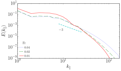
Figure 1: (Color online) Reduced parallel energy spectrum $E(k_{\parallel})$ for the three simulations with isotropic forcing. A $k_{\parallel}^{-3}$ slope is shown only as a reference.

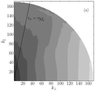
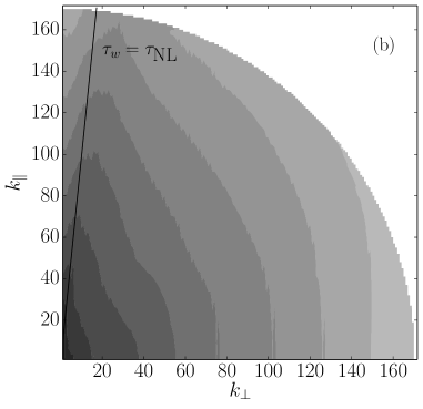
Figure 2: (Color online) Space resolved axisymmetric energy spectrum $e(k_{\perp},k_{\parallel})$ for two runs with (a) $\textrm{Fr}\approx 0.02$, and (b) $\textrm{Fr}\approx 0.01$. Note the spectral anisotropy resulting from stratification. The solid line indicates the modes with wave period equal to the eddy turnover time, $\tau_{\omega}=\tau_{\textrm{NL}}$. In (b) a ridge is formed close to this curve, indicating energy is transferred towards modes with lower $k_{\perp}$ but the transfer is halted when $\tau_{\omega}\approx\tau_{NL}$. Modes with $\tau_{\omega}<\tau_{\textrm{NL}}$ (i.e., modes below the solid line) are often called wave modes, as these modes have the wave period as the fastest timescale. However, a proper characterization of waves requires space and time resolved spectra.

IV Results

IV.1 Spatial spectral analysis

Traditional characterization of turbulent flows is done using one-dimensional spectra. In Fig. 1 we present the parallel spectrum $E(k_{\parallel})$ for the three simulations with isotropic forcing. Only as a reference, we also show in Fig. 1 a power law $\propto k_{\parallel}^{-3}$. The reader can find detailed spatial characterizations of stratified turbulence, which go beyond the aim of this work and at higher spatial resolution, in recent studies (see, e.g., Waite and Bartello (2006); Brethouwer et al. (2007)).

As a better way to characterize energy distribution among scales in the presence of anisotropy, Fig. 2 shows the spatial axisymmetric energy spectrum $e(k_{\perp},k_{\parallel})$, normalized by $\sin\theta$ with $\theta=\arctan(k_{\perp}/k_{\parallel})$ to obtain circular isocountours in the case of an isotropic flow. In Fig. 2, two spectra are presented, for the simulations with isotropic forcing and $\textrm{Fr}\approx 0.02$ and $\approx 0.01$. As stratification is increased, energy distribution becomes more anisotropic, with energy being preferentially transferred towards modes with smaller $k_{\perp}$ (and, as a result, larger wave period) Billant and Chomaz (2001); Waite and Bartello (2006); Brethouwer et al. (2007); Smith and Waleffe (2002). However, for $\textrm{Fr}\approx 0.01$ energy accumulates near the modes with wave period ($\tau_{\omega}\propto 1/\omega_{0}$) equal to the nonlinear turnover time ($\tau_{\textrm{NL}}\propto L/u_{\textrm{rms}}$), forming a ridge. As the energy transfer mechanism is often given by the shortest timescale Clark di Leoni et al. (2014), modes below the curve $\tau_{\omega}=\tau_{\textrm{NL}}$ (those with wave period shorter than the turnover time) are associated with waves Smith and Waleffe (2002); Waite and Bartello (2006); Brethouwer et al. (2007). Modes above the curve $\tau_{\omega}=\tau_{\textrm{NL}}$ (and in particular, modes with $k_{\perp}=0$) are often called vortical modes, as for these modes $\omega_{0}\approx 0$. The fraction of the energy in these modes decreases with decreasing Fr, in good agreement with the observed accumulation near $\tau_{\omega}=\tau_{\textrm{NL}}$ for large Fr. The slow down of the transfer as the energy reaches the ridge is compatible with critical balance arguments Nazarenko (2011), and is also of great importance in weak wave turbulence theories Lvov and Tabak (2001) that require the energy of the system to remain in weakly interacting waves. Note however that this distinction between waves and vortical modes in Fig. 2, based on the characteristic time of each mode, is only approximate. A strict discrimination between waves and eddies requires the four-dimensional spectrum.

IV.2 Spatio-temporal analysis

Precise identification of the waves, and of their role in the dynamics, requires both space and time information. Figure 3 shows different cuts of the frequency and wavenumber spectrum $E_{\theta}(k_{x},k_{y},k_{z},\omega)$ for $k_{x}=0$, and for either $k_{z}=0$ or $k_{z}=10$ in the simulation with the strongest stratification and isotropic forcing. As internal gravity waves couple vertical motions with temperature fluctuations, we consider the spectrum of potential energy $E_{\theta}$ to isolate the waves more easily. In Fig. 3 there is no significant accumulation of energy in the modes that satisfy the dispersion relation given by Eq. (3), i.e., in modes that could be directly associated with internal gravity waves. Instead, most of the energy ($\approx 80\%$ for $k_{y}\in[10,80]$) falls inside a wider region defined by the Doppler shifted Eq. (5) with $-0.4\leq U_{y}\leq 0.4$. This suggests the waves are propagating through layers with non-zero mean horizontal velocity (i.e., VSHW). Indeed, a probability density function (PDF) of the Cartesian components of the horizontally averaged horizontal velocity ${\bf U}$ obtained directly from the same simulation shows two peaks at $\approx\pm 0.4$ (see the inset in Fig. 4). Also, the PDF of the point-wise horizontal velocity in the entire box is approximately Gaussian with variance close to $0.4$.

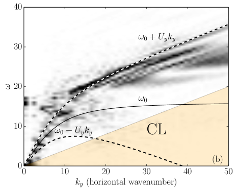
Figure 3: (Color online) Space and time resolved spectrum of the potential energy $E_{\theta}(k_{x}=0,k_{y},k_{z},\omega)$ (normalized by $E({\bf k})$, with 0 corresponding to white and $1$ corresponding to black), for $\textrm{Fr}=0.01$, and for two different values of $k_{z}$: (a) $k_{z}=0$, and (b) $k_{z}=10$. The fundamental dispersion relation $\omega_{0}({\bf k})$ from Eq. (3) is given by the thin solid curve, along with two Doppler shifted branches with $U_{y}=\pm 0.4$ (dashed curves). Energy is mostly concentrated in the fan defined by the two shifted branches, although not uniformly distributed. Waves that travel with the flow (upper half fan) concentrate most of the power. The area shaded with transparent orange corresponds to $\omega<U_{y}k_{y}$ with $U_{y}=0.4$; note there is almost no power in this region. The defect of energy in all modes in this area indicates these waves are absorbed by critical layers (CL), with their energy being transferred to the flow. Inset: Fraction of the energy $F$ that is contained within the two Doppler shifted branches as a function of the wavenumber. In the inertial range, $\approx 80\%$ of the energy corresponds to Doppler shifted waves.

It is important to remind that we force the fluid from rest at the large scales; this generates the winds, and by nonlinear interactions energy cascades towards the smaller scales. Then, the cycle completes itself when the small scale waves interact with the large scale winds; we are not imposing flows at different scales, or imposing a background flow, as sometimes done to study interaction of waves with shear flows. Instead, we just let turbulent interactions develop by themselves. In similar simulations of turbulent stratified flows, waves have been directly observed before by measuring the frequency spectrum $E(\omega)$, or by measuring $E(\omega)$ for a few Fourier modes Lindborg and Brethouwer (2007). This study identified peaks at the frequency of the internal gravity waves, but from the frequency spectrum a relation between frequency $\omega$ and wavenumber ${\bf k}$ cannot be obtained without assuming the system is dominated by the waves (and then the relation of these quantities is given by the dispersion relation), or dominated by vortical motions (and then the relation is given by sweeping, see, e.g., Clark di Leoni et al. (2014)).

Figure 3 gives direct evidence that most of the energy is in waves. And the waves satisfy Eq. (5) where ${\bf U}$ is the horizontal wind. However, there is more power in modes close to the curve $\omega_{0}+U_{y}k_{y}$ (with $U_{y}=0.4$) than in modes close to $\omega_{0}-U_{y}k_{y}$. This energy distribution cannot be explained by a preferential direction in ${\bf U}$ (see the PDFs in the inset in Fig. 4), by viscous effects (which introduce damping but no frequency shift), or by nonlinear corrections to the dispersion relation, as internal gravity waves are exact nonlinear solutions of the Boussinesq equations Majda (2003). The preferential concentration is instead compatible with a CL instability. In Fig. 3 we show as a reference the area (shaded in transparent gray or orange) where $\omega<U_{y}k_{y}$ with $U_{y}=0.4$. As in this simulation $-0.4\lesssim U_{y}\lesssim 0.4$ (once again, see the PDFs in the inset in Fig. 4), for all modes in that area there is some layer with $U_{y}$ such that the layer can be a CL. When the waves approach these layers, $c\approx U$, and from Eq. (6) their vertical velocity starts fluctuating more rapidly, undergoing an instability and transferring a fraction of their energy to the flow Hines (1991); Winters and D’Asaro (1994) (i.e., the waves are absorbed). Indeed, there is almost no energy in the wave modes in this area. This mechanism can only act if $\textrm{Ri}>1/4$. We verified the point-wise value of Ri in the simulations is larger than $1/4$. For the run with $\textrm{Fr}\approx 0.04$, the minimum of Ri is $\approx 14$. Although this value is rather large for atmospheric flows, it has been reported in other simulations of stratified turbulence, and indicate that CL instability can be the reason for the nonlocal formation of large scale structures in stratified turbulence observed in Smith and Waleffe (2002); Marino et al. (2013, 2014).

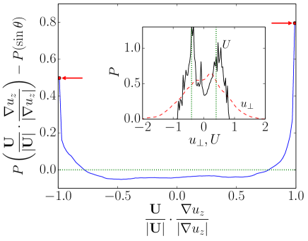
Figure 4: (Color online) Probability density function for horizontal gradients of the vertical velocity being aligned or anti-aligned with the mean horizontal flow, minus the probability of having uniformly distributed alignment between the fields ($\theta$ is uniformly distributed in $[0,2\pi)$). The PDF indicates (independently of Fig. 3) that there is an excess of waves traveling with the mean horizontal flow (compared with against the flow), and also a defect of waves propagating perpendicular to the flow. Inset: Probability distribution of the Cartesian components of the mean horizontal velocity ${\bf U}$, and of the point-wise horizontal velocity ${\bf u}_{\perp}$. The dotted vertical lines indicate the values $\pm 0.4$, used to draw the Doppler shifted branches in Fig. 3.

Internal gravity waves in a stratified fluid couple the temperature with the vertical component of the velocity. We now show that the four-dimensional power spectrum of the vertical velocity displays the same features as the spectrum of the potential energy shown above. Figure 5 shows a cut of the power spectrum of the vertical velocity $E_{z}(k_{x}=0,k_{y},k_{z}=0,\omega)$ in the simulation with stronger stratification and isotropic forcing. The same features found in the four-dimensional spectrum of the potential energy can be found in this figure, including the Doppler shift and the defect of energy in the modes that have frequency compatible with CL instability. In fact, the spectra are practically indistinguishable. As in the case of the temperature, a large fraction of the energy in vertical motions is also associated with wave motions, ($\approx 80\%$ of the energy between $10<k_{y}<80$ is inside the fan corresponding to Doppler shifted waves, see the inset in Fig. 5). When the spectrum of horizontal velocity is considered instead, none of these signatures can be found (not shown).

As a final and independent verification of the excess of waves traveling with the flow observed in Fig. 3, we resort to a statistical analysis. As most of the energy in the simulation with $\textrm{Fr}\approx 0.01$ is in the waves, we can assume the vertical velocity is a superposition of traveling waves $\propto e^{i({\bf k}\cdot{\bf x}-\omega t)}$. We can then compute ${\bf U}\cdot{\bf\nabla}u_{z}/(|{\bf U}||{\bf\nabla}u_{z}|)$, which gives an estimation of how the wave vector (i.e., the propagation direction for a pure planar wave) is aligned with the horizontal flow. Figure 4 shows the PDF of this alignment (averaged over every layer in the fluid) minus the PDF of the sine of a uniformly distributed angle $\theta\in[0,2\pi)$ (i.e., of randomly aligned fields with no privileged direction), for the simulation with stronger stratification and isotropic forcing. The result indicates a preference towards an alignment of horizontal gradients of the vertical velocity with the mean flow, as there is an excess for $+1$ when compared with $-1$, and a deficit (compared with uniformly distributed angles) for the case in which the two fields are perpendicular. Interestingly, a preference of stratified flows towards developing one sign of velocity gradients (resulting in non-Gaussian PDFs) was reported before in Rorai et al. (2013).

An interesting fact, that sheds more light on how these mechanisms work, is that these effects are not observed in purely rotating flows Clark di Leoni et al. (2014); Yarom and Sharon (2014). While these flows can also generate strong horizontal velocity fields, waves tend to travel in the vertical direction (as compared to the stratified case, where they tend to travel horizontally), and no Doppler shift develops as the waves are perpendicular to the large-scale flow.

IV.3 Dependence on level of stratification and forcing

The results discussed so far correspond to the simulation with randomly generated isotropic forcing and $\textrm{Fr}\approx 0.01$. A similar distribution of energy in frequency and wavenumber is observed in the simulations with same forcing but with higher Fr (i.e., weaker stratification), although the excess of waves traveling with the flow (as well as the defect in the fan defined by the CL) is stronger in the flow with smallest Fr. Figures showing the dependence with Froude number are shown below. For Taylor-Green forcing, which prevents the formation of a mean wind in each horizontal layer, the CL instability is not observed, although Doppler spreading of the waves still takes place. These results are also presented in this section.

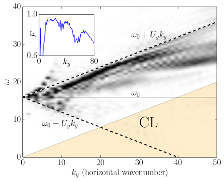
Figure 5: (Color online) Space and time resolved spectrum of vertical kinetic energy $E_{z}(k_{x}=0,k_{y},k_{z}=10,\omega)$, normalized by $E_{z}({\bf k}$), and for $\textrm{Fr}=0.01$. There is no discernible difference with the space and time spectrum of the potential temperature (see Fig. 3). The solid line corresponds to the linear dispersion relation of gravity waves, while the dashed lines indicate the two Doppler shifted dispersion relations with $U_{y}=\pm 0.4$. The region shaded with transparent orange indicates the modes that can have a CL instability, note the lack of energy in that region. Inset: Fraction of the energy $F$ that is contained within the two Doppler shifted branches as a function of the wavenumber.

As a comparison with the case shown in Fig. 3, Fig. 6(a) shows the space and time resolved spectrum $E_{\theta}(k_{x}=0,k_{y},k_{z}=0,\omega)$ for a simulation still forced with randomly generated forcing, but with $\textrm{Fr}\approx 0.02$. This spectrum can be directly compared with Fig. 3(a). Decreasing the stratification results in a spectrum that bears great resemblance with the spectrum for $\textrm{Fr}\approx 0.01$, with non-uniform Doppler spreading of the waves and the excess of waves with $\omega\approx\omega_{0}+U_{y}k_{y}$. The defect of energy in the modes compatible with CL instability is also visible in this simulation, although the damping of these modes is slightly weaker than in the case with stronger stratification. This is compatible with the smaller fraction of energy in the waves as stratification is decreased; see the inset of Fig. 6(a). Also, this is compatible with the fact that as stratification is decreased, the power in the large-scale motions (small wavenumbers) also decreases (see Fig. 1). These trends are further confirmed by the simulation with weaker stratification and $\textrm{Fr}\approx 0.04$.

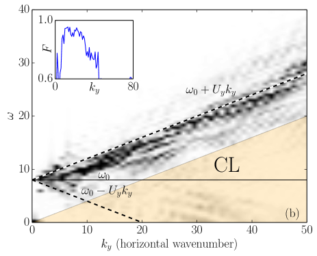
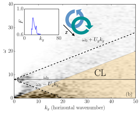
Figure 6: (Color online) Space and time resolved spectrum of the potential energy $E_{\theta}(k_{x}=0,k_{y},k_{z}=10,\omega)$ (normalized by $E_{\theta}({\bf k}$) for $\textrm{Fr}=0.02$, and for two different forcing functions: (a) isotropic forcing, and (b) Taylor-Green forcing. Labels are as in Fig. 5. The insets show in each case the fraction of the energy $F$ that is contained within the two Doppler shifted branches. In (b), the inset on the right also shows a schematic representation of the Taylor-Green forcing. In (a), note the decrease in the level of stratification of the system still preserves the main features of the spectrum. In (b), they Taylor-Green forcing injects most of the energy in vortical modes ($\omega\approx 0$), the energy in the waves is therefore smaller, and the flow geometry prevents the CL instability from developing.

When Taylor-Green forcing is used instead, the broadening of the dispersion relation by Doppler shift can still be observed; see Fig. 6(b) for $\textrm{Fr}\approx 0.02$, specially for wavenumbers $0<k_{y}\lesssim 10$. However, this effect is dimmed by a large concentration of energy in modes with $\omega\approx 0$. This is to be expected as the Taylor-Green forcing, given by ${\bf F}=f_{0}(\sin x\cos y\cos z\,\hat{x}-\cos x\sin y\cos\,\hat{z})$, consists of two counter rotating vortices in the horizontal velocity, and excites no vertical motions directly (see a schematic diagram in the inset of Fig. 6(b)). As a result, the fraction of energy in wave modes is much smaller than in the case with isotropic forcing (see also a direct measurement of this in the inset of Fig. 6(b)). Moreover, the imposition of the Taylor-Green vortices in each layer by the external forcing seems to disrupt the development of a non-zero mean wind in each horizontal layer, weakening also the development of the CL instability. Indeed, the damping of the energy in modes consistent with CL instability in the four-dimensional spectrum of potential energy in Fig. 6(b) is almost inexistent.

To ease with the understanding of the behavior caused by the two different forcings, and to illustrate the presence of VSHW in the flows, in Fig. 7 we present vertical slices (at constant $x$) of the potential temperature and horizontal velocity fields for the two simulations. Although the simulations have the same Fr and Re, the flows are significantly different. On the one hand, there are smaller scale structures and overturning in both fields for the Taylor-Green forced simulation. On the other hand, the simulation with isotropic forcing shows a more dominant large-scale horizontal flow, and smaller scale (although smoother) fluctuations in the temperature. This is consistent with the fact that when forcing isotropically there is more energy in the waves, as seen in Fig. 6. Another way to quantify how much energy is in the VSHW is to compare the ratio of the energy in the modes with $\omega=0$ (i.e., in the modes with $k_{\perp}=0$) to the total energy. For $\textrm{Fr}=0.02$, the Taylor-Green simulation has $\approx 0.009\%$ of its total energy in those modes, while the isotropically forced one has $\approx 0.03\%$, indicating that the isotropically forced simulation has stronger VSHW. Note however that both simulations have a broad energy spectrum, indicating that turbulence in both flows may be of different nature, with the case with more energy in wave motions being smoother and possibly closer to a wave turbulence regime.

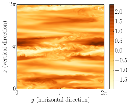
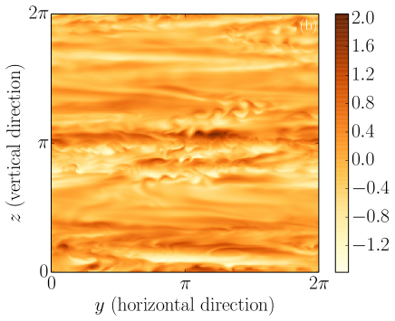
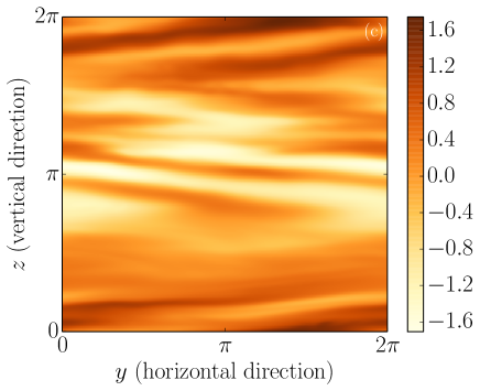
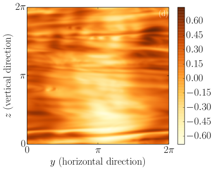
Figure 7: Vertical cuts (at constant $x$) of the potential temperature $\theta$, and of the $y$-component of the velocity field $u_{y}$, for simulations with the same $\textrm{Fr}=0.02$ but with different forcing functions. Panels (a) and (b) correspond to Taylor-Green forcing: (a) $u_{y}(y,z)$, and (b) $\theta(y,z)$. Panels (c) and (d) correspond to isotropic forcing: (c) $u_{y}(y,z)$, and (d) $\theta(y,z)$. Note the more evident horizontal winds in the simulation with isotropic forcing, and the different nature of the fluctuations in the temperature in both flows.

The comparison between the two different forcing functions further indicates that stratified turbulent flows may display different behavior depending on whether the mechanism used to excite the turbulence allows or prevents the development of large-scale vertically sheared horizontal winds. Interestingly, the case studied here that injects more energy directly into the waves, is also the case in which horizontal winds and CL instability more clearly develop, two features that are not considered in wave turbulence theories.

V Conclusions

In a turbulent flow, waves and individual instability events cannot be easily identified. As a result, previous numerical and observational studies of Doppler shift and CL instability focused on analyzing single wave packets travelling through a background flow. Our analysis, based on computation of a four-dimensional spectrum with high temporal and spatial resolution, allowed us to study these phenomena in turbulent flows, and to identify direct evidence of their occurrence.

With these tools we showed that Doppler shift and CL instability occur naturally in a stratified disordered flow, as a result of the interaction of the waves with the horizontal winds. This indicates the CL instability can be one of the mechanism behind the formation of large scales structures in stratified flows, often observed in simulations but whose origin is unclear Smith and Waleffe (2002); Marino et al. (2013, 2014). Moreover, although Doppler shift is observed in all forcing functions considered, development of the CL instability requires the external forcing not to disrupt the development of mean horizontal winds. Theories of stratified wave turbulence should take these effects into account. The mechanism, and the tools presented here, can be also relevant in quasi-geostrophic turbulence James (1987) and plasma turbulence Diamond et al. (2005); Connaughton et al. (2011), where zonal flows are also known to develop.