Error Floor Analysis of Coded Slotted ALOHA over Packet Erasure Channels

Abstract

We present a framework for the analysis of the error floor of coded slotted ALOHA (CSA) for finite frame lengths over the packet erasure channel. The error floor is caused by stopping sets in the corresponding bipartite graph, whose enumeration is, in general, not a trivial problem. We therefore identify the most dominant stopping sets for the distributions of practical interest. The derived analytical expressions allow us to accurately predict the error floor at low to moderate channel loads and characterize the unequal error protection inherent in CSA.

I Introduction

Coded slotted ALOHA (CSA) has recently been proposed as an uncoordinated multiple access technique that can provide large throughputs close to those of coordinated schemes [1, 2]. The need for CSA arises in scenarios where high throughput is required and coordinated techniques cannot be used due to various reasons, such as random number of devices in machine-to-machine communication. In this work, we assume a scenario where, besides throughput considerations, reliability plays an important role. We therefore focus on the probability of communication failure as our main figure of merit [3].

Different versions of CSA have been proposed (see [4] for the most recent review). All of them share a slotted structure borrowed from the original slotted ALOHA [5] and the use of successive interference cancellation. The contending users introduce redundancy by encoding their messages into multiple packets, which are transmitted to the base station (BS) in randomly chosen slots. The BS buffers the received signal, decodes the packets from the slots with no collision and attempts to reconstruct the packets in collision exploiting the introduced redundancy. A packet that is reconstructed is subtracted from the buffered signal and the BS proceeds with another round of decoding.

The analysis of CSA is usually done assuming that a packet in a collision-free slot can be reliably decoded and the interference caused by a packet can be ideally subtracted if the packet is known. Under these assumptions, the system can be viewed as a graph-based code operating over a binary erasure channel (BEC). Most papers on CSA consider error-free transmission. Here, we consider transmission over the packet erasure channel (PEC) [6]. The PEC can be used to model packets that are erased due to a deep fade for a block fading channel in the large signal-to-noise ratio (SNR) regime. It can also be used to model a network with random connectivity.

The BEC model allows us to use density evolution (DE) to predict the asymptotic performance of the system when the frame length tends to infinity. The typical performance exhibits a threshold behavior, i.e., all users are reliably resolved if the number of users does not exceed a certain threshold. Most of the work on CSA focuses on optimizing the threshold. However, the performance in the finite frame length regime is more relevant in practice. Similarly to low-density parity-check (LDPC) codes, a finite frame length gives rise to an error floor due to stopping sets present in the graph [7]. For regular CSA, some simple approximations to predict the error floor were proposed in [8]. In this paper, we derive analytical expressions to predict the error floor for irregular CSA [9] over the PEC. The derived expressions also allow us to predict the unequal error protection (UEP) inherent in irregular CSA. Moreover, we show that the asymptotic analysis using DE fails for systems operating over the PEC.

II System Model

We consider $m$ users that transmit to the BS over a shared medium. The communication takes place during a contention period called frame, consisting of $n$ slots of equal duration. Using a properly designed physical layer, each user maps its message to a physical layer packet and then repeats it $l$ times ($l$ is a random number chosen based on a predefined distribution) in randomly chosen slots, as shown in Fig. 1LABEL:sub@fig:system_model_a. This setup can be viewed as repetition coding and such a user is called a degree-$l$ user. Every packet contains pointers to its copies, so that, once a packet is successfully decoded, full information about the location of the copies is available.

(a) Time representaion of CSA.

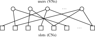
(b) Graph representation of CSA.

Figure 1: System model.

The received signal at the BS in the $i$th slot is

$$y_{i}=\sum_{j\in\mathcal{U}_{i}}h_{i,j}a_{j},$$ (1)

where $a_{j}$ is a packet of the $j$th user, $h_{i,j}$ is the channel coefficient and $\mathcal{U}_{i}\subset\{1,\dots,m\}$ is the set of users that transmit in the $i$th slot. We assume the channel coefficients to be independent across users and slots and identically distributed such that $\mathrm{Pr}\left\{|h_{i,j}|=0\right\}=\epsilon$ and $\mathrm{Pr}\left\{|h_{i,j}|>0\right\}=1-\epsilon$, i.e., $\epsilon$ is the probability of a packet erasure. We refer to such a channel as a PEC. If the number of nonzero coefficients $h_{i,j}\neq 0$ for $j\in\mathcal{U}_{i}$ is one, the $i$th slot is called a singleton slot. Otherwise, we say that a collision occurs in the $i$th slot.

At first the BS decodes the packets in singleton slots and obtains the location of their copies. Using data-aided methods, the channel coefficients corresponding to the copies are then estimated. After subtracting the interference caused by the identified copies, decoding proceeds until no further singleton slots are found. The PEC also models the capture effect since a packet in the $i$th slot may be decoded even if $|\mathcal{U}_{i}|>1$.

The system can be analyzed using the theory of codes on graphs over the BEC. Each user corresponds to a variable node (VN) and represents a repetition code, whereas slots correspond to check nodes (CNs) and can be seen as single parity-check codes. In the following, users and VNs are used interchangeably. An edge connects the $j$th VN to the $i$th CN if $j\in\mathcal{U}_{i}$ and $h_{i,j}\neq 0$. For the example in Fig. 1LABEL:sub@fig:system_model_a, the corresponding bipartite graph is shown in Fig. 1LABEL:sub@fig:system_model_b. A bipartite graph is defined as $\mathcal{G}=\{\mathcal{V},\mathcal{C},\mathcal{E}\}$, where $\mathcal{V}$, $\mathcal{C}$, and $\mathcal{E}$ represent the sets of VNs, CNs, and edges, respectively. The performance of the system greatly depends on the distribution that users use to choose the degree $l$ or, using graph terminology, on the VN degree distribution

$$\tilde{\lambda}(x)=\sum_{l=0}^{q}\tilde{\lambda}_{l}x^{l},$$ (2)

where $x$ is a dummy variable, $\tilde{\lambda}_{l}$ is the probability of choosing degree $l$, and $q$ is the maximum degree, which is often bounded due to implementation constraints, for instance, by eight in [9]. We define a vector representation of (2) as $\bm{\tilde{\lambda}}=[\tilde{\lambda}_{0},\dots,\tilde{\lambda}_{q}]$. For a graph $\tilde{\mathcal{G}}$ generated using $\bm{\tilde{\lambda}}$, we define the graph profile as the vector $\bm{v}(\tilde{\mathcal{G}})=[v_{0}(\tilde{\mathcal{G}}),v_{1}(\tilde{\mathcal{G}}),\dots,v_{q}(\tilde{\mathcal{G}})]$, where $v_{l}(\tilde{\mathcal{G}})$ is the number of degree-$l$ VNs in $\tilde{\mathcal{G}}$. The profile of a random graph $\tilde{\mathcal{G}}$ has a distribution $\mathrm{Pr}\left\{\bm{v}(\tilde{\mathcal{G}})=\bm{u}\right\}=p_{\mathsf{mn}}(\bm{u},\bm{\tilde{\lambda}},m)$, where

$$p_{\mathsf{mn}}(\bm{u},\bm{\tilde{\lambda}},m)=\begin{cases}m!\prod_{l=0}^{q}\frac{\tilde{\lambda}_{l}^{u_{l}}}{u_{l}!}&\text{if }\|\bm{u}\|_{1}=m,\\ 0&\text{otherwise}\end{cases}$$ (3)

is the multinomial distribution and $\|\cdot\|_{1}$ is the $\ell_{1}$ norm.

The key performance parameters are defined as follows. The channel load $g=m/n$ shows how “busy” the medium is. The average number of users that successfully transmit their message, termed resolved users, is denoted by $r$. The throughput $t=r/n$ shows how efficiently the frame is used. In this paper, we focus on the average packet loss rate (PLR) $\mathrm{bar}{p}=(m-r)/m=1-t/g$, which is the fraction of unresolved users, i.e., the users whose messages are not successfully decoded by the BS.

III Performance Analysis

Let a user repeat its packet $l$ times. Each copy is erased with probability $\epsilon$. Hence, the BS receives $k\in\{0,\dots,l\}$ packets with probability $\binom{l}{k}\epsilon^{l-k}(1-\epsilon)^{k}$. Averaging over the VN degree distribution $\tilde{\lambda}(x)$ leads to the induced VN degree distribution $\lambda(x)$ observed by the BS

$$\lambda(x)=\sum_{l=0}^{q}\tilde{\lambda}_{l}\sum_{k=0}^{l}\binom{l}{k}\epsilon^{l-k}(1-\epsilon)^{k}x^{k},$$ (4)

which can be written similarly to (2), where

$$\lambda_{l}=\sum_{k=l}^{q}\binom{k}{l}\epsilon^{k-l}(1-\epsilon)^{l}\tilde{\lambda}_{k}$$ (5)

is the fraction of users of degree $l$ as observed by the BS. The PEC can thus be analyzed by considering $\lambda(x)$ over a standard collision channel [9]. The main peculiarity of the induced distribution, not considered in the standard CSA analysis, is that it contains all degrees up to $q$, including zero and one. This implies that the PLR exhibits an error floor, which is lowerbounded by $\lambda_{0}=\tilde{\lambda}(\epsilon)>0$ for $\epsilon>0$. Hence, the threshold, i.e., the channel load below which the PLR is zero when $n\rightarrow\infty$, predicted by DE is zero over a PEC with $\epsilon>0$ for any distribution $\tilde{\lambda}(x)$. Moreover, DE devised in [9] does not correspond to the decoding algorithm for distributions with $\lambda_{1}\neq 0$. In the following, we focus on the induced distribution $\lambda(x)$ and the induced graph $\mathcal{G}=\{\mathcal{V},\mathcal{C},\mathcal{E}\}$.

By construction CSA features UEP, similarly to the UEP in coding theory, since users with different degrees are protected differently. The inherent UEP is illustrated by dashed lines in Fig. 3LABEL:sub@fig:num_res_e0 for $\tilde{\lambda}(x)=0.25x^{2}+0.6x^{3}+0.15x^{8}$ and $\epsilon=0$. As clearly seen from the figure, the higher the degree, the better the PLR performance. We remark that the performance of a degree-$l$ user depends on the entire distribution and not only on its degree. To characterize the performance of users of different degrees, we define the PLR for a degree-$l$ user as observed by the BS as

$$p_{l}=\frac{\mathrm{bar}{w}_{l}}{\mathrm{bar}{m}_{l}}=\frac{\mathrm{bar}{w}_{l}}{m\lambda_{l}},$$ (6)

where $\mathrm{bar}{m}_{l}$ and $\mathrm{bar}{w}_{l}$ are the average number of all and unresolved degree-$l$ users, respectively. For degree-$0$ users, $p_{0}=1$. The average PLR is

$$\mathrm{bar}{p}=\frac{1}{m}\sum_{l=0}^{q}{\mathrm{bar}{w}_{l}}=\sum_{l=0}^{q}{\lambda_{l}p_{l}}.$$ (7)

Since packet erasures are accounted for in the induced distribution, the only source of errors in the considered model is harmful structures in the graph $\mathcal{G}$. When, e.g., two degree-$2$ users transmit in the same slots (see Fig. 2LABEL:sub@fig:two_two), the BS will not be able to resolve them. Such harmful structures are commonly referred to as stopping sets. A subset of VNs of non-zero degrees $\mathcal{S}\subset\mathcal{V}$ forms a stopping set if all neighbors of $\mathcal{S}$ are connected to $\mathcal{S}$ at least twice [7]. $\mathcal{S}$ induces a graph, which, with a slight abuse of notation, is also referred to as stopping set and denoted by $\mathcal{S}$. Therefore, $\mathcal{S}$ can be described by its profile $\bm{v}(\mathcal{S})$. For $\mathcal{S}_{2}$ in Fig. 2LABEL:sub@fig:type2, the graph profile is $\bm{v}(\mathcal{S}_{2})=[0,2,1,0,\dots,0]$, where the number of zeros in the end depends on $q$.

(a) $\mathcal{S}_{1}$.

(b) $\mathcal{S}_{2}$.

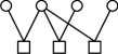
(c) $\mathcal{S}_{3}$.

(d) $\mathcal{S}_{4}$.

(e) $\mathcal{S}_{5}$.

(f) $\mathcal{S}_{6}$.

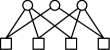
(g) $\mathcal{S}_{7}$.

(h) $\mathcal{S}_{8}$.

Figure 2: Stopping sets.

Stopping sets are referred to as “loops” in [8]. However, stopping sets do not form a loop if degree-$1$ users are present, as in Fig. 2LABEL:sub@fig:type1–LABEL:sub@fig:type4. On the other hand, if there are no degree-$1$ users, all stopping sets create cycles (or loops) in the graph, as in Fig. 2LABEL:sub@fig:two_two–LABEL:sub@fig:type8. Length-$4$ cycles are the shortest cycles possible and are always avoided in properly designed LDPC codes. Due to the randomly generated graph, however, length-$4$ cycles are intrinsic to CSA.

We denote the probability of a stopping set $\mathcal{S}$ to occur by $\rho(\mathcal{S})$. Let $\mathcal{A}$ be the set of all possible stopping sets. Using a union bound argument, the number of unresolved degree-$l$ users can be upperbounded as

$$\mathrm{bar}{w}_{l}\leq\sum_{\mathcal{S}\in\mathcal{A}}{v_{l}(\mathcal{S})\rho(\mathcal{S})}.$$ (8)

The probability $\rho(\mathcal{S})$ is in general difficult to evaluate. In the following, we give an example to show how it can be approximated. Consider $\mathcal{S}_{5}$ in Fig. 2LABEL:sub@fig:two_two and assume a particular realization of $\mathcal{G}$ so that $v_{2}(\mathcal{G})\geq 2$. Numerical results show that for low channel loads, the probability to observe exactly one stopping set $\mathcal{S}_{5}$ is at least one order of magnitude larger than the probability of any other possible stopping set formed by degree-$2$ users (including multiple $\mathcal{S}_{5}$) to occur. We therefore assume that only one stopping set $\mathcal{S}_{5}$ occurs. This also hints that $\mathcal{S}_{5}$ is the most dominant among all stopping sets containing only degree-$2$ users. Users of other degrees may transmit in the same slot as the users in $\mathcal{S}_{5}$. This may create a new larger stopping set, or these users may be successfully resolved and their interference subtracted. However, the users in $\mathcal{S}_{5}$ will remain unresolved. Each of the degree-$2$ users has $\gamma=\binom{n}{2}$ possible combinations of slots for transmission. Given that the number of slots is large enough for the realization of $\mathcal{G}$ ($\gamma\geq v_{2}(\mathcal{G})$), we write

$$\rho(\mathcal{S}_{5},\mathcal{G})\approx\alpha(\mathcal{S}_{5},\mathcal{G})\beta(\mathcal{S}_{5},\mathcal{G}),$$ (9)

where

$$\alpha(\mathcal{S}_{5},\mathcal{G})=\binom{v_{2}(\mathcal{G})}{2}$$ (10)

and

$$\beta(\mathcal{S}_{5},\mathcal{G})=\frac{1}{\gamma^{v_{2}(\mathcal{G})}}\!\!\prod_{k=0}^{v_{2}(\mathcal{G})-2}\!\!(\gamma-k)=\frac{\gamma!}{(\gamma-v_{2}(\mathcal{G})+1)!\gamma^{v_{2}(\mathcal{G})}},$$

where the right-hand side of (9) is the probability of one stopping set $\mathcal{S}_{5}$ to occur and is split into a product of two variables for future use.

In the following, we remove the dependency on $\mathcal{G}$ from (9) in order to obtain $\rho(\mathcal{S}_{5})$. To do so, we simplify $\beta(\mathcal{S}_{5},\mathcal{G})$ assuming that $\gamma\gg v_{2}(\mathcal{G})$. By letting $\gamma$ grow large, we obtain $\beta(\mathcal{S}_{5},\mathcal{G})\approx\beta(\mathcal{S}_{5})=\gamma^{-1}$. The same result can be obtained setting $v_{2}(\mathcal{G})$ to the minimal possible value, i.e., two. To find $\rho(\mathcal{S}_{5})$, $\alpha(\mathcal{S}_{5},\mathcal{G})$ in (10) needs to be averaged over all $\mathcal{G}$, i.e., $\alpha(\mathcal{S}_{5})=\mathsf{E}_{\mathcal{G}}\left\{\alpha(\mathcal{S}_{5},\mathcal{G})\right\}$, where $\mathsf{E}_{\mathcal{G}}\left\{\cdot\right\}$ stands for the expectation over $\mathcal{G}$.

For a generic $\mathcal{S}$, (10) generalizes to

$$\alpha(\mathcal{S},\mathcal{G})=\prod_{l=1}^{q}\binom{v_{l}(\mathcal{G})}{v_{l}(\mathcal{S})}.$$ (11)

Using (11) and the definition of the multinomial distribution in (3), $\alpha(\mathcal{S})=\mathsf{E}_{\mathcal{G}}\left\{\alpha(\mathcal{S},\mathcal{G})\right\}$ can be calculated as

$$\alpha(\mathcal{S})=\binom{m}{\|\bm{v}(\mathcal{S})\|_{1}}p_{\mathsf{mn}}(\bm{v}(\mathcal{S}),\bm{\lambda},\|\bm{v}(\mathcal{S})\|_{1}).$$ (12)

We apply the reasoning above to all stopping sets and write

$$\rho(\mathcal{S})\approx\alpha(\mathcal{S})\beta(\mathcal{S}),$$ (13)

where $\beta(\mathcal{S})$ is the probability of the stopping set $\mathcal{S}$ to occur in a graph with profile $\bm{v}(\mathcal{S})$, and $\alpha(\mathcal{S})$ is the number of combinations to choose $v_{l}(\mathcal{S})$ users out of $v_{l}(\mathcal{G})$ users present in the graph $\mathcal{G}$ for all degrees, averaged over $\mathcal{G}$. The numerical results presented later on justify the approximation in (13).

Identifying all stopping sets and calculating the corresponding $\beta(\mathcal{S})$ in a systematic way is not possible in general. In practice, distributions with large fractions of low-degree VNs are most commonly used since they achieve high thresholds. For instance, the soliton distribution [10], which asymptotically provides throughput arbitrarily close to one, has $\tilde{\lambda}_{2}=0.5$ and $\tilde{\lambda}_{3}=0.17$. If we constrain ourselves to the family of such distributions, i.e., distributions with large fractions of degree-$2$ and degree-$3$ users, identifying the most dominant stopping sets becomes possible. By running extensive simulations for different distributions from the aforementioned family of distributions for $g=0.5$, we determined the stopping sets that contribute the most to the error floor by estimating their relative frequencies. These stopping sets are shown in Fig. 2, with

$$\beta(\mathcal{S}_{1})=\frac{1}{n},\beta(\mathcal{S}_{2})=\frac{2}{n^{2}},\beta(\mathcal{S}_{3})=\frac{6}{n^{3}},\beta(\mathcal{S}_{4})=\frac{6}{(n-1)n^{2}},$$

$$\beta(\mathcal{S}_{5})=\frac{2}{(n-1)n},\beta(\mathcal{S}_{6})=\!\frac{4(n-3)}{(n\!-\!2)n^{3}},$$ (14)

$$\beta(\mathcal{S}_{7})=\frac{36(n-3)}{(n-2)(n-1)n^{3}},\beta(\mathcal{S}_{8})=\frac{6}{(n-2)(n-1)n}.$$

Note that constraining the set of the considered stopping sets turns the upper bound in (8) into an approximation. The PLR of a degree-$l$ user can thus be approximated as

$$p_{l}\approx\frac{1}{m\lambda_{l}}\sum_{\mathcal{S}\in\mathcal{A}_{8}}{v_{l}(\mathcal{S})\alpha(\mathcal{S})\beta(\mathcal{S})},$$ (15)

where $\mathcal{A}_{8}$ is the set of the eight stopping sets in Fig. 2 with the corresponding $\alpha(\mathcal{S})$ in (12) and $\beta(\mathcal{S})$ in (14).

The analysis above is presented for the induced degree distribution, i.e., $p_{l}$ in (6) is the PLR for a user of degree $l$ as observed by the BS. The PLR for a degree-$l$ user (from the user’s perspective) can be found as

$$\tilde{p}_{l}=\sum_{k=0}^{l}p_{k}\binom{l}{k}\epsilon^{l-k}(1-\epsilon)^{k}$$ (16)

if $\tilde{\lambda}_{l}\neq 0$ and zero otherwise. When $\epsilon=0$, it is easy to see from (5) that $\tilde{\lambda}_{l}=\lambda_{l}$ and from (16) that $\tilde{p}_{l}=p_{l}$ for all $l={0,\dots,q}$. We remark that calculating (16) is not required if we are interested in the average PLR, i.e., it can be calculated based on $p_{l}$ and $\lambda(x)$ as in (7).

IV Numerical Results

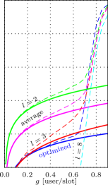
(a) $\epsilon=0$.

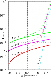
(b) $\epsilon=0.03$.

Figure 3: The PLR performance for $n=200$. Dashed lines show simulation results and solid lines show analytical error floor approximations (16).

In Fig. 3, we plot the PLR for a degree-$l$ user (from the user’s perspective) for $\tilde{\lambda}(x)=0.25x^{2}+0.6x^{3}+0.15x^{8}$ and two different values $\epsilon$. This distribution was suggested in [9] as a distribution that provides low error floor. The dashed lines show the simulation results and the solid lines show the proposed analytical PLR expression (16) based on the approximation (15). The analytical PLR predictions demonstrate good agreement with the simulation results for low to moderate channel loads. This justifies the approximation in (13) and the use of the stopping sets in Fig. 2. Considering other stopping sets can improve the PLR prediction for higher channel loads and would make it possible to predict the performance of users of higher degrees. However, as Fig. 3 suggests, the contribution of these users to the average PLR is negligible, especially in the error floor region. We also remark that the accuracy of the approximations improves when the frame length increases. In Fig. 3LABEL:sub@fig:num_res_e003, we also show the value of $\lambda_{0}=\tilde{\lambda}(0.03)=2.4\times 10^{-4}$ to demonstrate the lower bound on the average PLR.

The proposed PLR approximation can also be used for the optimization of the degree distribution. As an example, we performed the optimization for $n=200$ and $\epsilon=0$ using a linear combination of the threshold provided by DE and the analytical prediction of the average PLR as the objective function. One of the obtained distributions is $\tilde{\lambda}(x)=0.87x^{3}+0.13x^{8}$ and its average PLR performance is shown with blue lines in Fig. 3LABEL:sub@fig:num_res_e0. This distribution has considerably lower error floor without significant degradation of the performance in the waterfall region compared to the distribution from [9].

V Conclusions

In this letter, we proposed analytical approximations of the error floor of CSA for finite frame length over the PEC. These approximations show good agreement with simulation results for most distributions of practical interest. The approximations can be used to optimize the degree distribution for a given frame length and packet erasure probability.

References

- [1] E. Paolini, G. Liva, and M. Chiani, “High throughput random access via codes on graphs: Coded slotted ALOHA,” in Proc. IEEE Int. Conf. Commun., Kyoto, Japan, June 2011.
- [2] C. Stefanovic and P. Popovski, “ALOHA random access that operates as a rateless code,” IEEE Trans. Commun., vol. 61, no. 11, pp. 4653–4662, Nov. 2013.
- [3] G. C. Madueno, C. Stefanovic, and P. Popovski, “Reliable reporting for massive M2M communications with periodic resource pooling,” IEEE Wireless Comm. Letters, vol. 3, no. 4, pp. 429–432, Aug. 2014.
- [4] E. Paolini, G. Liva, and M. Chiani, “Coded slotted ALOHA: A graph-based method for uncoordinated multiple access,” submitted to IEEE Trans. Inf. Theory, Jan. 2014, available at http://arxiv.org/abs/1401.1626.
- [5] L. G. Roberts, “ALOHA packet system with and without slot and capture,” SIGCOMM Comput. Commun. Rev., vol. 5, no. 2, pp. 28–42, Apr. 1975.
- [6] A. Guillén i Fàbregas, “Coding in the block-erasure channel,” IEEE Trans. Inf. Theory, vol. 52, no. 11, pp. 5116–5121, Nov. 2006.
- [7] C. Di, D. Proietti, I. E. Telatar, T. J. Richardson, and R. L. Urbanke, “Finite-length analysis of low-density parity-check codes on the binary erasure channel,” IEEE Trans. Inf. Theory, vol. 48, no. 6, pp. 1459–1473, June 2002.
- [8] O. D. R. Herrero and R. D. Gaudenzi, “Generalized analytical framework for the performance assessment of slotted random access protocols,” IEEE Trans. Wireless Commun., vol. 13, no. 2, pp. 809–821, Feb. 2014.
- [9] G. Liva, “Graph-based analysis and optimization of contention resolution diversity slotted ALOHA,” IEEE Trans. Commun., vol. 59, no. 2, pp. 477–487, Feb. 2011.
- [10] K. R. Narayanan and H. D. Pfister, “Iterative collision resolution for slotted ALOHA: an optimal uncoordinated transmission policy,” in Proc. Int. Symp. on Turbo Codes and Iterative Information Processing, Gothenburg, Sweden, Aug. 2012.