Circumventing the Curse of Dimensionality in Prediction:
Causal Rate-Distortion for
Infinite-Order Markov Processes

Abstract

Predictive rate-distortion analysis suffers from the curse of dimensionality: clustering arbitrarily long pasts to retain information about arbitrarily long futures requires resources that typically grow exponentially with length. The challenge is compounded for infinite-order Markov processes, since conditioning on finite sequences cannot capture all of their past dependencies. Spectral arguments show that algorithms which cluster finite-length sequences fail dramatically when the underlying process has long-range temporal correlations and can fail even for processes generated by finite-memory hidden Markov models. We circumvent the curse of dimensionality in rate-distortion analysis of infinite-order processes by casting predictive rate-distortion objective functions in terms of the forward- and reverse-time causal states of computational mechanics. Examples demonstrate that the resulting causal rate-distortion theory substantially improves current predictive rate-distortion analyses.

Keywords: optimal causal filtering, computational mechanics, epsilon-machine, causal states, predictive rate-distortion, information bottleneck

I Introduction

Biological organisms and engineered devices are often required to predict the future of their environment either for survival or performance. Absent side information about the environment that is inherited or hardwired, their only guide to the future is the past. One strategy for adapting to environmental challenges, then, is to memorize as much of the past as possible—a strategy that ultimately fails, even for simple stochastic environments, due to the exponential growth in required resources.

One way to circumvent resource limitations is to identify maximally predictive features in a time series, coarse-graining pasts into partitions with equivalent conditional probability distributions over futures. These partitions are minimal sufficient statistics for prediction, known as the forward-time causal states $\mathcal{S}^{+}$ of computational mechanics, and storing them costs on average $C_{\mu}^{+}=\operatorname{H}[{\mathcal{S}}^{+}]$ bits [1, 2]. For processes with finite $C_{\mu}^{+}$ [3, 4] identifying the causal states obviates storing an exponentially growing number of sequences. However, for many processes, perhaps most [5, 6], $C_{\mu}^{+}$ is infinite and so storing the causal states themselves exceeds the capacity of any learning strategy.

As such, one asks for approximate, lossy features that predict the future as well as possible given resource constraints. Shannon introduced rate-distortion theory to analyze such trade-offs [7, 8], encoding an information source so that “the maximum possible signaling rate is obtained without exceeding the tolerable distortion level”. When applied to prediction, rate-distortion theory provides a principled framework for calculating the function delineating achievable from unachievable predictive distortion for a given amount of memory. Such rate-distortion functions are used to test, for instance, whether or not a biological sensory system extracts lossy predictive features [9]. In other applications, optimal codebooks identify useful features for understanding and building approximate predictive models of complex datasets [10, 11, 12, 13, 14] and define natural predictive macrostates of a stochastic process [15, 16].

Unfortunately, current methods for calculating rate-distortion functions for prediction require clustering arbitrarily long pasts to obtain information about arbitrarily long futures, incurring the very resource limitations one hoped to avoid. They can be avoided for some classes of simple process, when there is an analytic expression for the joint past-future probability distribution [17, 11, 18]. In practice, though, one compresses finite-length pasts to retain information about finite-length futures [15, 16]. This will yield reasonable estimates of predictive rate-distortion functions at sufficient lengths, but how long is long enough?

To address this practical problem and, more generally, to circumvent resource limitations, we identify a new relationship between predictive rate-distortion theory and causal states. This gives an alternative theory and class of algorithms for calculating predictive rate-distortion functions, when a maximally predictive model is identified first. Revisiting previous results [15, 16], the alternative demonstrates that identifying a maximally predictive model first dramatically improves rate-distortion analysis for even the simplest stochastic processes. A natural hierarchy of phase transitions associated with discovering new predictive features emerges as a function of approximation error, paralleling those described in Ref. [19]. As an illustration, we calculate a predictive “hierarchy” for a process generated by a complex chaotic dynamical system.

Section II reviews computational mechanics and predictive rate-distortion theory. Section III describes how current predictive rate-distortion algorithms encounter the curse of dimensionality. Section IV introduces a theorem that reformulates predictive rate-distortion analysis in terms of forward- and reverse-time causal states. Section V then describes a new algorithm for computing lossy causal states and illustrates its performance on infinite-order Markov processes. Section VII summarizes outstanding issues, desirable extensions, and future applications.

II Background

When an information source’s entropy rate falls below a channel’s capacity, Shannon’s Second Coding Theorem says that there exists an encoding of the source messages such that the information can be transmitted error-free, even over a noisy channel. What happens, though, when the source rate is above this error-free regime? This is what Shannon solved by introducing rate-distortion theory [7, 8].

II.1 Problem Statement

Our view is that, for natural systems, the above-capacity regime is disproportionately more common and important than the original error-free coding with which Shannon and followers started. This is certainly the circumstance in which most of measurement science finds itself. Instrumentation almost never exactly captures an experimental system’s states exactly. One can argue that this is even guaranteed by quantum uncertainty relations. Similarly for biological life and engineered adaptive systems, their sensory apparatus does not capture all of an environment’s information and organization. Indeed, in many cases they cannot due to sensory limitations. Even without such limitations, moreover, they may not have adequate representational capacity.

And, perhaps more profoundly, one does not want to do perfectly, as the “stammering grandeur” of Irenio Funes reminds us [20, Funes The Memorious]. Said positively, summarizing sensory information not only helps reduce demands on memory, but also the computational complexity of downstream perceptual processing, cognition, and acting. For instance, much effort has been focused on determining memory and the ability to reproduce a given time series [21], but that memory may only be important to the extent that it affects the ability to predict the future; e.g., see Ref. [5, 22]. A decision that is adaptive for an organism can be quite simple, requiring only a coarse sketch of the environmental state: Individual Dictyostelium discoideum slime mold cells track only the concentration gradient of cyclic-AMP when moving to organize into a collective fruiting bud [23]. Moreover, many human perceptual models are rooted in identifying informative environmental features [24]. Experiments suggest there are constraints on the total number of features that humans can identify [25]—a psychological variant of the coding problem tackled by rate-distortion theory, but in a different asymptotic limit. We are interested, therefore, as others have been, in identifying lossy causal states.

First, we review causal states. Second, we review several information measures of stochastic processes. These, finally, lead us to describe what we mean by lossy causal states. The following assumes familiarity with information theory at the level of Ref. [26, 27], information theory for complex processes at the level of Refs. [28, 29], and computational mechanics at the level of Ref. [4].

II.2 Processes and Their Causal States

When predicting a system the main object is the process $\mathcal{P}$ it generates: the list of all of a system’s behaviors or realizations $\{\ldots{x}_{-2},{x}_{-1},{x}_{0},{x}_{1},\ldots\}$ as specified by their joint probabilities $\Pr(\ldots{X}_{-2},{X}_{-1},{X}_{0},{X}_{1},\ldots)$. We denote a contiguous chain of random variables as ${X}_{0:\ell}={X}_{0}{X}_{1}\cdots{X}_{\ell-1}$. Left indices are inclusive; right, exclusive. We suppress indices that are infinite. In this setting, the present ${X}_{t:t+\ell}$ is the length-$\ell$ chain beginning at $t$, the past is the chain ${X}_{:t}=\ldots{X}_{t-2}{X}_{t-1}$ leading up the present, and the future is the chain following the present ${X}_{t+\ell:}={X}_{t+\ell+1}{X}_{t+\ell+2}\cdots$. When being more expository, we use arrow notation; for example, for the past $\smash{\overleftarrow{{X}}}={X}_{:0}$ and future $\smash{\overrightarrow{{X}}}={X}_{0:}$. We will refer on occasion to the space $\smash{\overleftarrow{{\rm{\bf{X}}}}}$ of all pasts. Finally, we assume a process is ergodic and stationary—$\Pr({X}_{0:\ell})=\Pr({X}_{t:\ell+t})$ for all $t\in\mathbb{Z}$—and the measurement symbols ${x}_{t}$ range over a finite alphabet: ${x}\in\mathcal{A}$. We make no assumption that the symbols represent the system’s states—they are at best an indirect reflection of an internal Markov mechanism. That is, the process a system generates is a hidden Markov process [30].

Forward-time causal states $\mathcal{S}^{+}$ are minimal sufficient statistics for predicting a process’s future [1, 2]. This follows from their definition as sets of pasts grouped by the equivalence relation $\sim^{+}$:

$${x}_{:0}\sim^{+} {x}_{:0}^{\prime}$$

$$\Leftrightarrow\Pr({X}_{0:}|{X}_{:0}={x}_{:0})=\Pr({X}_{0:}|{X}_{:0}={x}_{:0}^{\prime})~{}.$$ (1)

As a shorthand, we denote a cluster of pasts so defined, a causal state, as $\sigma^{+}\in\mathcal{S}^{+}$. We implement Eq. (1) via the causal state map: $\sigma^{+}=\epsilon^{+}({\smash{\overleftarrow{{x}}}})$. Through it, each state $\sigma^{+}$ inherits a probability $\pi(\sigma^{+})$ from the process’s probability over pasts $\Pr({X}_{:0})$. The forward-time statistical complexity is defined as the Shannon entropy of the probability distribution over forward-time causal states [1]:

$$C_{\mu}^{+}=\operatorname{H}[\mathcal{S}^{+}]~{}.$$ (2)

A generative model—the process’s $\epsilon$-machine—is built out of the causal states by endowing the state set with a transition dynamic:

$$T_{\sigma\sigma^{\prime}}^{x}=\Pr(\mathcal{S}_{t+1}^{+}=\sigma^{\prime},{X}_{t}={x}|\mathcal{S}_{t}^{+}=\sigma)~{},$$

matrices that give the probability of generating the next symbol ${x}_{t}$ and ending in the next state $\sigma_{t+1}$, if starting in state $\sigma_{t}$. (Since output symbols are generated during transitions there is, in effect, a half time-step difference in index. We suppress notating this.) For a discrete-time, discrete-alphabet process, the $\epsilon$-machine is its minimal unifilar Hidden Markov Model (HMM) [1, 2]. (For general background on HMMs see Refs. [31, 32, 33]. For a mathematical development of $\epsilon$-machines see Ref. [34].) Note that the causal-state set of a process generated by even a finite HMM can be finite, countable, or uncountable. Minimality can be defined by either the smallest number of causal states or the smallest statistical complexity $C_{\mu}$ [2]. Unifilarity is a constraint on the transition matrices such that the next state $\sigma_{t+1}$ is determined by knowing the current state $\sigma_{t}$ and the next symbol ${x}_{t}$.

A similar equivalence relation can be applied to find minimal sufficient statistics for retrodiction [35]. Futures are grouped together if they have equivalent conditional probability distributions over pasts:

$${x}_{0:}\sim^{-} {x}_{0:}^{\prime}$$

$$\Leftrightarrow\Pr({X}_{:0}|{X}_{0:}={x}_{0:})=\Pr({X}_{:0}|{X}_{0:}={x}_{0:}^{\prime})~{}.$$ (3)

A cluster of futures—a reverse-time causal state—defined by $\sim^{-}$ is denoted $\sigma^{-}\in\mathcal{S}^{-}$. Again, each $\sigma^{-}$ inherits a probability $\pi(\sigma^{-})$ from the probability over futures $\Pr({X}_{0:})$. And, the reverse-time statistical complexity is the Shannon entropy of the probability distribution over reverse-time causal states:

$$C_{\mu}^{-}=\operatorname{H}[\mathcal{S}^{-}]~{}.$$ (4)

In general, the forward- and reverse-time statistical complexities are not equal [35, 36]. That is, different amounts of information must be stored from the past (future) to predict (retrodict). Their difference $\Xi=C_{\mu}^{+}-C_{\mu}^{-}$ is a process’s causal irreversibility and it reflects this statistical asymmetry.

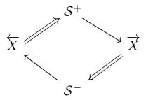
Figure 1: Computational Mechanics Markov Loop [35, 37]: Markov chain relationships between the past, future, and causal states ${\mathcal{S}}^{+}$ and ${\mathcal{S}}^{-}$. Relations: $\Rightarrow$ denotes “function of”, and $\rightarrow$ denotes being part of Markov chain.

Here, the most important aspect of forward- and reverse-time causal states are that they “shield” the past and future from one another. That is:

$$\Pr(\smash{\overleftarrow{{X}}},\smash{\overrightarrow{{X}}}|\mathcal{S}^{+}) =\Pr(\smash{\overleftarrow{{X}}}|\mathcal{S}^{+})\Pr(\smash{\overrightarrow{{X}}}|\mathcal{S}^{+})\text{ and }$$

$$\Pr(\smash{\overleftarrow{{X}}},\smash{\overrightarrow{{X}}}|\mathcal{S}^{-}) =\Pr(\smash{\overleftarrow{{X}}}|\mathcal{S}^{-})\Pr(\smash{\overrightarrow{{X}}}|\mathcal{S}^{-})~{},$$

even though $\mathcal{S}^{+}$ and $\mathcal{S}^{-}$ are functions of $\smash{\overleftarrow{{X}}}$ and $\smash{\overrightarrow{{X}}}$, respectively. Figure 1 illustrates shielding the future $\smash{\overrightarrow{{X}}}$ from the past $\smash{\overleftarrow{{X}}}$, given by the forward causal states $\mathcal{S}^{+}$, and the past from the future, given by the reverse causal states $\mathcal{S}^{-}$. The result is a series of Markov chains forming a Markov loop that illustrates the relationship between prediction and retrodiction.

II.3 Information Measures

To measure a process’s asymptotic per-symbol uncertainty one uses the Shannon entropy rate:

$$h_{\mu}=\lim_{\ell\to\infty}\frac{\operatorname{H}(\ell)}{\ell}~{},$$

when the limit exists and where $\operatorname{H}(\ell)=-\sum_{w\in\mathcal{A}^{\ell}}\Pr(w)\log_{2}\Pr(w)$ is the block entropy. $h_{\mu}$ measures the rate at which a stochastic process generates information. From standard informational identities, one sees that the entropy rate is also given by the conditional entropy:

$$h_{\mu}=\lim_{\ell\to\infty}\operatorname{H}[{X}_{0}|{X}_{-\ell:0}]~{}.$$ (5)

This form makes transparent its interpretation as the residual uncertainty in a measurement given the infinite past. As such, it is often employed as a measure of a process’s degree of unpredictability. The maximum amount of information in the future that is predictable from the past (or vice versa) is the excess entropy:

$${\bf E} =\operatorname{I}[{X}_{:0};{X}_{0:}]~{}.$$

It is symmetric in time and a lower bound on the stored information: ${\bf E}\leq C_{\mu}$.

More generally, Shannon’s various information quantities—entropy, conditional entropy, mutual information, and the like—when applied to processes are functions of the joint distributions $\Pr({X}_{0:\ell})$. Importantly, they define an algebra of information measures for a given set of random variables [27]. Reference [29] used this to show that the past and future partition the single-measurement entropy $\operatorname{H}({X}_{0})$ into several distinct measure-theoretic atoms. These are useful in particular to answer the question posed by the Introduction, how long is long enough to capture all of a process’s correlations? For this, we use the amount of predictable information not captured by the length-$\ell$ present:

$$\sigma_{\mu}(\ell)=\operatorname{I}[{X}_{:0};{X}_{\ell:}|{X}_{0:\ell}]~{}.$$ (6)

This is the elusive information [38], which measures the amount of past-future correlation not contained in the present. It is a decreasing function of the present’s length $\ell$. It is nonzero if a process necessarily has hidden states and is therefore quite sensitive to how a system’s internal state space is observed or coarse grained. For example, an order-$R$ Markov process has $\sigma_{\mu}(\ell)=0$ for $\ell\geq R$. In this case, $R$-blocks serve as a process’s effective states, rendering the past and future independent—shielding them from each other. Note, however, that in the space of processes generated by finite HMMs, infinite-order Markov processes dominate overwhelmingly [39]. For these, $\sigma_{\mu}(\ell)$ vanishes only asymptotically. The excess entropy itself is lower-bounded by the elusive information: $\sigma_{\mu}(\ell)\leq{\bf E}$. In fact, $\sigma_{\mu}(0)={\bf E}$.

Finally, the following refers to finite-length variants of causal states and finite-length estimates of statistical complexity and ${\bf E}$. For example, the latter is given by:

$${\bf E}(M,N)=\\ I[{X}_{-M:0};{X}_{0:N}]~{}.$$ (7)

If ${\bf E}$ is finite, then ${\bf E}=\lim_{M,N\rightarrow\infty}{\bf E}(M,N)$. Processes generated by finite-state HMMs have finite ${\bf E}$—they are finitary processes [28]. When ${\bf E}$ is infinite, then the way in which ${\bf E}(M,N)$ diverges is one measure of a process’ complexity [40, 41, 28]. An analogous, finite past-future $(M,N)$-parametrized equivalence relation leads to finite-length causal states—${\mathcal{S}}^{+}_{M,N}$ and ${\mathcal{S}}^{-}_{M,N}$—and statistical complexities—$C_{\mu}^{+}(M,N)=\operatorname{H}[{\mathcal{S}}^{+}_{M,N}]$ and $C_{\mu}^{-}(M,N)=\operatorname{H}[{\mathcal{S}}^{-}_{M,N}]$.

The quality of a process’s approximation can be monitored by the convergence error ${\bf E}-{\bf E}(M,N)$, which is controlled by the elusive information $\sigma_{\mu}(\ell)$. To see this, we apply the mutual information chain rule repeatedly:

$${\bf E} =\operatorname{I}[{X}_{:0};{X}_{0:}]$$

$$=\operatorname{I}[{X}_{:0};{X}_{0:N-1}]+\sigma_{\mu}(N)$$

$$={\bf E}(M,N)+\operatorname{I}[{X}_{:-M-1};{X}_{0:N-1}|{X}_{-M-1:0}]+\sigma_{\mu}(N)~{}.$$

The last mutual information is difficult to interpret, but easy to bound:

$$\operatorname{I}[{X}_{:-M-1};{X}_{0:N-1} |{X}_{-M-1:0}]$$

$$\leq\operatorname{I}[{X}_{:-M-1};{X}_{0:}|{X}_{-M-1:0}]$$

$$=\sigma_{\mu}(M)~{},$$

And so, the convergence error is upper-bounded by the elusive information:

$$0\leq{\bf E}-{\bf E}(M,N)\leq\sigma_{\mu}(N)+\sigma_{\mu}(M)~{}.$$ (8)

II.4 Lossy Causal States

Lossy causal states are naturally defined via predictive rate-distortion (PRD) or its information-theoretic instantiations, optimal causal inference (OCI) [15, 16] and the past-future information bottleneck (PFIB) [11]. This section briefly reviews rate-distortion theory, but interested readers should refer to Refs. [7, 8, 42] or Ref. [27, Ch. 8] for detailed expositions. The presentation here is adapted to serve our focus on prediction.

Figure 2(top) shows the rate-distortion theory setting of Ref. [27] that combines the encoder and noisy channel used in Shannon’s communication channel model [7, 8] into a single encoder. This is often a more appropriate framing for biological information processing [9] where a sensory system (e.g., retina) both distorts the input signal (e.g., natural scenery) and transmits codewords that convey information about the input signal to the next information processing post (e.g., the lateral geniculate nucleus).

Figure 2: (top) Rate-distortion setting: Using a codebook an encoder maps input sequences into codewords. A decoder then estimates the source sequence from the codewords. (bottom) Optimal Causal Inference [15, 16]: Markov chain relationships between the past, future, and lossy predictive features $\mathcal{R}_{\beta}$. Relations: $\Rightarrow$ denotes “function of”, $\rightarrow$ denotes a Markov chain, and $Y\rightsquigarrow Z$ indicates that random variable $Z$ is the “relevant” variable for $Y$. The latter does not imply a Markov chain relationship.

In this framing, an information source generates $n$ successive symbols, a word ${x}_{0:n}\in\mathcal{A}^{n}$. The word is presented to the encoder, which outputs one of $M$ codewords $\{r_{i}:i=1,\ldots M\}$. The collection $\mathbb{C}=\{({x}_{0:n},r_{i}):i=1,\ldots,M\}$, mapping words to codewords, is the channel codebook. Since sending one of $M$ codewords requires $\log_{2}M$ bits, the code rate $R(\mathbb{C})=n^{-1}\log M$ is the number of communicated bits per source symbol.

Given a codeword $r_{i}$, the decoder makes its best estimate $\widehat{{x}}_{0:n}\in\mathcal{A}^{n}$ as to the original source word ${x}_{0:n}$. Each estimate is evaluated using a distortion measure $d({x}_{0:n},\widehat{{x}}_{0:n})\geq 0$, that quantifies the error between the given codeword $\widehat{{x}}_{0:n}$ and the true word ${x}_{0:n}$. Over long periods, the estimates lead to an expected distortion:

$$\mathbb{E}d({x},\widehat{{x}})=\lim_{n\rightarrow\infty}\frac{\mathbb{E}d({x}_{0:n},\widehat{{x}}_{0:n})}{n}~{},$$

that depends on the codebook $\mathbb{C}$ and its associated code rate $R(\mathbb{C})$. We assume that the distortion measure is normal: $\min_{\{\widehat{{x}}_{0:n}\}}d({x}_{0:n},\widehat{{x}}_{0:n})=0$.

There is a natural trade-off between the code rate and the expected distortion: the smaller the desired expected distortion, the larger the required code rate to achieve it. To achieve no expected distortion, $\mathbb{E}d({x},\widehat{{x}})=0$, requires some minimal code rate $R_{max}$, which depends on the distortion measure. For instance, when reconstructing a given time series as well as possible, $R_{max}$ is the process’s entropy rate $h_{\mu}$ [43]. When the information source consists of successive semi-infinite pasts $\smash{\overleftarrow{{X}}}$ of a time series, then for many prediction-related distortion measures, $R_{max}$ is the forward-time statistical complexity $C_{\mu}^{+}$ [2, 15, 16]. More generally, when the distortion measure is an informational distortion of a source $X$ with respect to some “relevant variable” $Y$ [44, 45], then $R_{max}$ is the entropy of the inherited probability distribution of the minimal sufficient statistics of $X$ with respect to $Y$ [46].

A channel’s capacity $\mathcal{C}$ is the largest information transmission rate it can sustain over all possible information sources $X$:

$$\mathcal{C}=\sup_{\Pr(X)}\operatorname{I}[X;Y]~{},$$

where $Y$ is the channel’s output process. If the encoder’s capacity is large enough—$\mathcal{C}\geq R_{max}$—then there exists a codebook such that the decoder can reconstruct the input sequence with arbitrarily small probability of error. If the encoder’s capacity is not large enough—$\mathcal{C}<R_{max}$—however, it cannot. There is an irreducible positive error rate. As the Introduction noted, for PRD applications one is in this regime when $C_{\mu}^{+}$ is infinite [6, 5].

In this positive error-rate regime, we ask for the rate-distortion function:

$$R(D)=\inf_{\mathbb{E}d({x},\widehat{{x}})\leq D}R(\mathbb{C})~{}.$$ (9)

For simplicity, we typically limit ourselves to single-symbol distortion measures, so that the distortion between decoded and input word is:

$$d({x}_{0:n},\widehat{{x}}_{0:n})=\sum_{i=0}^{n-1}d({x}_{i},\widehat{{x}}_{i})~{}.$$

Equation (9) is a difficult optimization, given that to determine $R(D)$ for each $D$ requires enumerating a combinatorially large space of codebooks. Instead, one views the information source as a random variable ${X}$ with realizations ${x}$ and the (potentially stochastic) codebook’s output as a random variable $\mathcal{R}=\mathbb{C}(X)$ with realizations $r\in\{1,\ldots,M\}$.

Then, according to the Rate-Distortion Theorem, one has:

$$R(D)=\min_{\langle d({x},r)\rangle_{{X},\mathcal{R}}\leq D}\operatorname{I}[{X};\mathcal{R}]~{}.$$

One can solve numerically for $R(D)$ using annealing to find a $\Pr(\mathcal{R}|{X})$ minimizing the objective function:

$$\mathcal{L}_{\beta}=\operatorname{I}[{X};\mathcal{R}]+\beta\langle d({x},r)\rangle_{{X},\mathcal{R}}~{}.$$

As $\beta$ varies, one obtains different rates $R_{\beta}=\operatorname{I}[{X};\mathcal{R}]$ and expected distortions $D_{\beta}=\langle d({x},r)\rangle_{{X},\mathcal{R}}$. In this way, one traces out the rate-distortion function $R(D)$ parametrically.

Note that, in the preceding, ${X}$ was not a measurement symbol of a stochastic process, as it was in Sec. II.2. In the present context, ${X}$ is the random variable denoting the output of any information source, which could be, but need not be, a string of symbols from a stochastic process.

A natural question arises, which distortion measure should one use? Historically, it was chosen to be a more or less familiar statistic, such as the mean-squared error and the like. More recently, though, information measures have been used, mirroring the definition of the code rate in the objective function. For example, Ref. [44] posited that one should retain some aspect $\mathcal{R}$ of the input ${X}$ that is related to another “relevant” random variable $Y$. This is tantamount to assuming a Markov chain relationship: $\mathcal{R}\to X\to Y$. A natural distortion measure then is [47]:

$$d({x},r)={D_{\textrm{KL}}}[\Pr(Y|{X}={x})||\Pr(Y|\mathcal{R}=r)]~{},$$

where ${D_{\textrm{KL}}}(P||Q)$ is the relative entropy between distributions $P$ and $Q$. Though, one might consider others based on the distance between the conditional probability distributions $\Pr(Y|{X}={x})$ and $\Pr(Y|\mathcal{R}=r)$. It is straightforward to show that:

$$\langle{D_{\textrm{KL}}}[\Pr(Y|{X}={x})||\Pr(Y|\mathcal{R}=r)]\rangle=\operatorname{I}[{X};Y|\mathcal{R}]~{},$$

since the Markov chain gives $\Pr(Y|X,\mathcal{R})=\Pr(Y|X)$. And, since $\operatorname{I}[{X};Y|\mathcal{R}]=\operatorname{I}[{X};Y]-\operatorname{I}[\mathcal{R};Y]$ due to the same Markov chain assumption, we define the information function:

$$R(I_{0})=\min_{\operatorname{I}[\mathcal{R};Y]\geq I_{0}}\operatorname{I}[{X};\mathcal{R}]~{},$$

with objection function:

$$\mathcal{L}_{\beta}=\operatorname{I}[\mathcal{R};Y]-\beta^{-1}\operatorname{I}[{X};\mathcal{R}]~{}.$$

Finding the $\Pr(\mathcal{R}|{X})$ that maximize $\mathcal{L}_{\beta}$ is the basis for the information bottleneck (IB) method [44, 45].

Since our focus is prediction, we have already decided that the information source is a process’s past $\smash{\overleftarrow{{X}}}$ with realizations ${\smash{\overleftarrow{{x}}}}$ and the relevant variable is its future $\smash{\overrightarrow{{X}}}$. We have the Markov chain $\mathcal{R}\to\smash{\overleftarrow{{X}}}\to\smash{\overrightarrow{{X}}}$. (See Fig. 2(bottom).) And, our distortion measures have the form:

$$d({\smash{\overleftarrow{{x}}}},r)=d(\Pr(\smash{\overrightarrow{{X}}}|\smash{\overleftarrow{{X}}}={\smash{\overleftarrow{{x}}}}),\Pr(\smash{\overrightarrow{{X}}}|\mathcal{R}=r))~{}.$$

The predictive rate-distortion function is then:

$$R(D)=\min_{\langle d({\smash{\overleftarrow{{x}}}},r)\rangle_{\smash{\overleftarrow{{X}}},\mathcal{R}}\leq D}\operatorname{I}[\mathcal{R};\smash{\overleftarrow{{X}}}]~{}.$$

Determining the optimal $\Pr(\mathcal{R}|\smash{\overleftarrow{{X}}})$ that achieve these limits is predictive rate distortion (PRD). If we restrict to informational distortions, such as $\operatorname{I}[\smash{\overleftarrow{{X}}};\smash{\overrightarrow{{X}}}|\mathcal{R}]$, we find the associated information function is:

$$R(I_{0})=\min_{\operatorname{I}[\mathcal{R};\smash{\overrightarrow{{X}}}]\geq I_{0}}\operatorname{I}[\mathcal{R};\smash{\overleftarrow{{X}}}]~{},$$ (10)

and its accompanying objective function is:

$$\mathcal{L}_{\beta}=\operatorname{I}[\mathcal{R};\smash{\overrightarrow{{X}}}]-\beta^{-1}\operatorname{I}[\smash{\overleftarrow{{X}}};\mathcal{R}]~{}.$$ (11)

Calculating the $\Pr(\mathcal{R}|\smash{\overleftarrow{{X}}})$ that maximize Eq. (11) constitutes optimal causal inference (OCI) [15, 16] or, for linear dynamical systems, the past-future information bottleneck [11]. We refer to these methods generally as the predictive information bottleneck (PIB), emphasizing that an information distortion measure for PRD has been chosen.

This choice of method name does lead to confusion since the recursive information bottleneck (RIB) introduced in Ref. [48] is an information bottleneck approach to predictive inference that does not take the form of Eq. (11). However, RIB is a departure from the original IB framework since its objective function explicitly infers lossy machines rather than lossy statistics [49].

Generally, rate-distortion analysis reveals how a process’s structure (captured in the associated codebooks) varies under coarse-graining, with the shape of the rate-distortion functions identifying those regimes in which smaller codebooks are good approximations. To implement this analysis, one graphs a process’s information function $R(I_{0})$ and its accompanying feature curve $(\beta,R_{\beta})$, corresponding to optimizing $\mathcal{L}_{\beta}$ above. Again, previous results established that the zero-distortion predictive features are a process’s causal states and so the maximal $R(I_{0})=C_{\mu}^{+}$ [15, 16] and this code rate occurs at an $I_{0}={\bf E}$ [35, 37].

Figure 2(bottom) illustrates how the approximately predictive states $\mathcal{R}_{\beta}$ are soft clusters of the past $\smash{\overleftarrow{{X}}}$ constrained by predicting the future $\smash{\overrightarrow{{X}}}$ at a fidelity controlled by $\beta$. The new notation introduced there to indicate which random variable is “relevant” will be useful for explaining Thm. 1 via Fig. 4(b).

III Curse of Dimensionality in Prediction

Let’s consider the performance of any PRD algorithm that clusters pasts of length $M$ to retain information about futures of length $N$. In the lossless limit, when these algorithms work, they find features that capture $\operatorname{I}[{X}_{-M:0};{X}_{0:N}]={\bf E}(M,N)$ of the total predictable information ${\bf E}$ at a coding cost of $C_{\mu}^{+}(M,N)$. As $M,N\to\infty$, they should recover the forward-time causal states with predictability ${\bf E}$ and coding cost $C_{\mu}^{+}$. Increasing $M$ and $N$ come with an associated computational cost, though: storing the joint probability distribution $\Pr({X}_{-M:0},{X}_{0:N})$ of past and future finite-length trajectories requires storing $|\mathcal{A}|^{M+N}$ probabilities.

More to the point, applying PRD algorithms at small distortions requires storing and manipulating a matrix of dimension $|\mathcal{A}|^{M}\times|\mathcal{A}|^{N}$. This leads to obvious practical limitations—the curse of dimensionality for prediction. For example, current computing is limited to matrices of size $10^{5}\times 10^{5}$ or less, thereby restricting rate-distortion analyses to $M,N\leq\log_{|\mathcal{A}|}10^{5}$. (Recall that this is an overestimate, since the sparseness of the sequence distribution is determined by a process’s topological entropy rate.) And so, even for a binary process, when $|\mathcal{A}|=2$, one is practically limited to $M,N\leq 16$. Notably, $M,N\leq 5$ are more often used in practice [10, 15, 16, 50, 51]. Finally, note that these estimates do not account for the computational costs of managing numerical inaccuracies when measuring or manipulating the vanishingly small sequence probabilities that occur at large $M$ and $N$.

These constraints compete against achieving good approximations of the information function: we require that ${\bf E}-{\bf E}(M,N)$ be small. Otherwise, approximate information functions provide a rather weak lower bound on the true information function for larger code rates. This has been noted before in other contexts, when approximating non-Gaussian distributions as Gaussians leads to significant underestimates of information functions [18]. This calls for an independent calibration for convergence. We address this by calculating ${\bf E}-{\bf E}(M,N)$ in terms of the transition matrix $W$ of a process’ mixed-state presentation. When $W$ is diagonalizable with eigenvalues $\{\lambda_{i}\}$, Ref. [52] provides the closed-form expression:

$${\bf E}-{\bf E}(M,N)=$$

$$\sum_{i:\lambda_{i}\neq 1}\frac{\lambda_{i}^{M}+\lambda_{i}^{N+1}-\lambda_{i}^{M+N+1}}{1-\lambda_{i}}\langle\delta_{\pi}|W_{\lambda_{i}}|H(W^{\mathcal{A}})\rangle,$$ (12)

where $\langle\delta_{\pi}|W_{\lambda_{i}}|H(W^{\mathcal{A}})\rangle$ is a dot product between the eigenvector $\langle\delta_{\pi}|W_{\lambda_{i}}$ corresponding to eigenvalue $\lambda_{i}$ and a vector $H(W^{\mathcal{A}})$ of transition uncertainties out of each mixed state. Here, $\pi$ is the stationary state distribution and $W_{\lambda_{i}}$ is the projection operator associated with $\lambda_{i}$. When $W$’s spectral gap $\gamma=1-\max_{i:\lambda_{i}\neq 1}|\lambda_{i}|$ is small, then ${\bf E}(M,N)$ necessarily asymptotes more slowly to ${\bf E}$. When $\gamma$ is small, then (loosely speaking) we need $M,N\sim\log_{1-\gamma}\frac{\epsilon}{\gamma}$, where $\epsilon$ is of order ${\bf E}-{\bf E}(M,N)$.

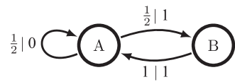
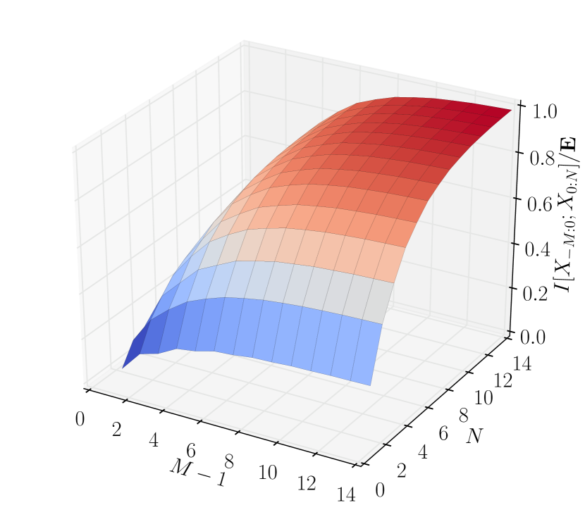
Figure 3: Curse of dimensionality when predicting the Even Process: (top) The $\epsilon$-machine, its minimal unifilar HMM. Edge labels $p|x$ denote generating symbol $x\in\mathcal{A}$ while taking the transition with probability $p$. (bottom) ${\bf E}(M,N)/{\bf E}$ as a function of $N$ and $M$ calculated exactly using Eq. (12) and the values of $\{\lambda_{i}\}$, $\langle\delta_{\pi}|W_{\lambda_{i}}|H(W^{\mathcal{A}})\rangle$ from App. I of Ref. [53]. The Even Process’s total predictable information ${\bf E}\approx 0.9183$ bits. Capturing $90\%$ of ${\bf E}$ requires: $M=6,~{}N\geq 13$ or $N=6,~{}M\geq 13$; $M=7,~{}N\geq 9$ or $N=7,~{}M\geq 9$; and $M\geq 8,N\geq 8$.

Figure 3(bottom) shows ${\bf E}(M,N)$ as a function of $M$ and $N$ for the Even Process, whose $\epsilon$-machine is displayed in the top panel. The process’s spectral gap is $\approx 0.3$ and, correspondingly, we see ${\bf E}(M,N)/{\bf E}$ asymptotes slowly to $1$. For example, capturing $90\%$ of the total predictable information requires $M,N\geq 8$. (The figure caption contains more detail on allowed $(M,N)$ pairs.) This, in turn, translates to requiring very good estimates of the probabilities of $\approx 10^{4}$ length-$16$ sequences. In Fig. $3$ of Ref. [16], by way of contrast, Even Process information functions were calculated using $M=3$ and $N=2$. As a consequence, the OCF estimates there captured only $27\%$ of the full ${\bf E}$.

The Even Process is generated by a simple two-state HMM, so it is notable that computing its information function (done shortly in Sec. V) is at all challenging. Then again, the Even Process is an infinite-order Markov process.

The difficulty can easily become extreme. Altering the Even Process’s lone stochastic transition probability can increase its temporal correlations such that correctly calculating its information function requires massive compute resources. Thus, the curse of dimensionality is a critical concern even for finite-$C_{\mu}$ processes generated by finite HMMs.

As we move away from such “simple” prototype processes and towards real data sets, the attendant inaccuracies generally worsen. Many natural processes in physics, biology, neuroscience, finance, and quantitative social science are highly non-Markovian with slowly asymptoting or divergent ${\bf E}$ [54]. This implies rather small spectral gaps if the process has a countable infinity of causal states—e.g., as in Ref. [55]—or a distribution of eigenvalues heavily weighted near $\lambda=0$, if the process has an uncountable infinity of causal states. In short, “interesting” processes [41] are those for which current information function algorithms are most likely to fail.

IV Causal Rate Distortion Theory

Circumventing the curse of dimensionality requires an alternative approach to predictive rate distortion (PRD)—causal rate distortion (CRD) theory—that leverages the structural information about a process captured by its forward and reverse causal states. Proposition 1, our first result, establishes that CRD is equivalent to PRD under certain conditions, leading to a new and efficient method to calculate information functions for a broad range of distortion measures. Our second result adapts CRD to informational distortions, introducing an efficient PIB alternative—causal information bottleneck (CIB). It shows that compressing $\smash{\overleftarrow{{X}}}$ to retain information about $\smash{\overrightarrow{{X}}}$ is equivalent to compressing $\mathcal{S}^{+}$ to retain information about $\mathcal{S}^{-}$. The results generalize two previous theorems of Refs. [15, 16, 35, 37]. This section first describes the relationship between PRD and CRD and then that between PIB and CIB in an intuitive way. Appendix A gives more precise statements and their proofs. Sec. V’s examples illustrate CRD’s benefits, partly by comparing to previous methods and partly through new analytical insights into information functions.

To start, inspired by the previous finding that PIB recovers the forward-time causal states in the zero-temperature ($\beta\to\infty$) limit [15, 16], we argue that compressing either the past $\smash{\overleftarrow{{X}}}$ or forward-time causal states $\mathcal{S}^{+}$ should yield the same predictive features at any temperature. This leads us to consider two different rate-distortion settings. In the first, traditional PRD setting we compress the past $\smash{\overleftarrow{{X}}}$ to minimize expected distortion about the future $\smash{\overrightarrow{{X}}}$. In the second, CRD setting we compress the forward-time causal states $\mathcal{S}^{+}$ to retain information about the future $\smash{\overrightarrow{{X}}}$. Though somewhat intuitive, there is no a priori reason that the two objective functions are related. The Markov chain of Fig. 4(top) lays out the implied interdependencies. For many distortion functions, in fact, they are not related. Lemma 1, however, says that they are equivalent for certain types of predictive distortion measures.

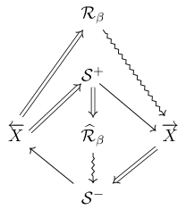
(a) Setting for Causal Rate Distortion Theory.
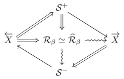
(b) Causal Rate Distortion’s Prop. 1 and Causal Information Bottleneck’s Thm. 1.

Figure 4: Causal Rate Distortion (CRD) Markov chain relationships between the past, future, causal states ${\mathcal{S}}^{+}$ and ${\mathcal{S}}^{-}$, and lossy predictive features $\mathcal{R}_{\beta}$ and $\widehat{\mathcal{R}}_{\beta}$. Diagrammatic notation as in Fig. 2(bottom).

Lemma 1.

Compressing the past $\smash{\overleftarrow{{X}}}$ to minimize expected predictive distortion is equivalent to compressing the forward-time causal states $\mathcal{S}^{+}$ to minimize expected predictive distortion if the distortion measure is expressible as $d(\Pr(\smash{\overrightarrow{{X}}}|\mathcal{R}=r),\Pr(\smash{\overrightarrow{{X}}}|\smash{\overleftarrow{{X}}}={\smash{\overleftarrow{{x}}}}))$.

Many distortion measures can be expressed in this form, though the mapping can be nonobvious. For instance, a distortion measure that penalizes the Hamming distance between the maximum likelihood estimates of the most likely future of length $L$ is actually expressible in terms of conditional probability distributions of futures given pasts or features. Lemma 1 then suggests that PRD will recover the forward-time causal states in the zero-temperature limit for a great many prediction-related distortion measures, not just the information distortions considered in Refs. [15, 16]. However, for distortion measures that ask for optimal predictions of an arbitrary coarse-graining of futures, the forward-time causal states will be no longer be sufficient statistics. Then, PRD’s zero-temperature limit will not recover the forward-time causal states.

Interestingly, in a nonprediction setting, Ref. [56] states Lemma 1 in their Eq. (2.2) without conditions on the distortion measure. At least in the context of PRD, this is an oversimplification. For instance, an entirely reasonable predictive distortion measure could penalize the difference between the output of a particular prediction algorithm applied to the true past versus an estimated past. Without proper conditions, these prediction algorithms can incorporate aspects of the past $\smash{\overleftarrow{{X}}}$ that are entirely useless for prediction. A version of Lemma 1 will still apply, but the variable that replaces $\smash{\overleftarrow{{X}}}$ depends on the particular prediction algorithm. For example, predictions of future sequences of the Even Process (Sec. III) based on certain ARIMA estimators will store unnecessary information about the past. This makes the forward-time causal states insufficient statistics with respect to the process and the predictor; see Sec. V.2. Ideally, prediction algorithms should tailored to the class of stochastic process to be predicted.

When the distortion measure takes a particular special form, then we can simplify the objective function further. Our inspiration comes from Refs. [35, 37, 57] which showed that the mutual information between past and future is identical to the mutual information between forward and reverse-time causal states: $\operatorname{I}[\smash{\overleftarrow{{X}}};\smash{\overrightarrow{{X}}}]=\operatorname{I}[\mathcal{S}^{+};\mathcal{S}^{-}]$. In other words, forward-time causal states $\mathcal{S}^{+}$ are the only features needed to predict the future as well as possible, and reverse-time causal states $\mathcal{S}^{-}$ are features one can predict about the future.

And so, we now consider a third objective function that compresses the forward-time causal states to minimize expected distortion about the reverse-time causal states. Proposition 1 says that this objective function is equivalent to compressing the past to minimize expected distortion for a class of distortion measures.

Proposition 1 (Causal Rate Distortion).

Compressing the past $\smash{\overleftarrow{{X}}}$ to minimize expected distortion of the future $\smash{\overrightarrow{{X}}}$ is equivalent to compressing the forward-time causal states $\mathcal{S}^{+}$ to minimize expected distortion of reverse-time causal states $\mathcal{S}^{-}$, if the distortion measure is expressible as:

$$d({\smash{\overleftarrow{{x}}}},r)=d(\Pr(\smash{\overrightarrow{{X}}}|\mathcal{R}=r),\Pr(\smash{\overrightarrow{{X}}}|\smash{\overleftarrow{{X}}}={\smash{\overleftarrow{{x}}}}))$$

and satisfies:

$$d(\Pr(\smash{\overrightarrow{{X}}}|\mathcal{R} =r),\Pr(\smash{\overrightarrow{{X}}}|\smash{\overleftarrow{{X}}}={\smash{\overleftarrow{{x}}}}))$$

$$=d(\Pr(\mathcal{S}^{-}|\mathcal{R}=r),\Pr(\mathcal{S}^{-}|\smash{\overleftarrow{{X}}}={\smash{\overleftarrow{{x}}}}))~{}.$$

Distortion measures that do not satisfy Prop. 1’s conditions, such as mean squared-error distortion measures, in effect emphasize predicting one reverse-time causal state over another. Even then, inferring a maximally-predictive model can improve calculational accuracy for nearly any distortion measure on sequence distributions. For details, see App. A.

Informational distortion measures, though, treat all reverse-time causal states equally. Leveraging this, Thm. 1 follows as a particular application of Prop. 1.

Theorem 1 (Causal Information Bottleneck).

Compressing the past $\smash{\overleftarrow{{X}}}$ to retain information about the future $\smash{\overrightarrow{{X}}}$ is equivalent to compressing $\mathcal{S}^{+}$ to retain information about $\mathcal{S}^{-}$.

Naturally, there is an equivalent version for the time reversed setting in which past and future are swapped and the causal state sets are swapped. Also, any forward and reverse-time prescient statistics [2] can be used in place of $\mathcal{S}^{+}$ and $\mathcal{S}^{-}$ in any of the statements above.

Appendix A’s proofs follow almost directly from the definitions of forward- and reverse-time causal states. Variations or portions of Lemma 1, Prop. 1, and Thm. 1 may seem intuitive. Appendix A points this out when clearly the case. That said, to the best of our knowledge, Lemma 1, Prop. 1, and Thm. 1 are new.

Theorem 1 and Prop. 1 reduce the numerically intractable problem of clustering in the infinite-dimensional space $(\smash{\overleftarrow{{X}}},\smash{\overrightarrow{{X}}})$ to the potentially tractable one of clustering in $\mathcal{S}^{\pm}$. This is beneficial when a process’s causal state set is finite. However, many processes have an uncountable infinity of forward-time causal states or reverse-time causal states [5, 6]. Is Theorem 1 useless in these cases? Not at all. A practical approach is that information functions can be approximated to any desired accuracy by a finite or countable $\epsilon$-machine. However, additional work is required to understand how model approximations map to information-function approximations.

V Examples

To illustrate CRD and CIB, we find lossy causal states and calculate information functions for processes generated by known $\epsilon$-machines. For several, the $\epsilon$-machines are sufficiently simple that the information functions can be obtained analytically using the above results. These allow us to comment more generally on the shape of information functions for several broad classes of process. The examples also provide a setting in which to compare CIB information functions to those from optimal causal filtering (OCF) [15, 16]. Though, Thm. 1 says that OCF and CIB yield identical results in the $L\rightarrow\infty$ limit, the examples give a rather sober illustration of the substantial errors that arise at finite $L$.

We display the results of the PRD analyses in two ways . The first is an information function that graphs the code rate $I[\smash{\overleftarrow{{X}}};\mathcal{R}]$ versus the distortion $I[\smash{\overleftarrow{{X}}};\smash{\overrightarrow{{X}}}|\mathcal{R}]$. The second is a feature curve of code rate $I[\smash{\overleftarrow{{X}}};\mathcal{R}]$ versus inverse temperature $\beta$. We recall that at zero temperature ($\beta\to\infty$) the code rate $I[\smash{\overleftarrow{{X}}};\mathcal{R}]=C_{\mu}^{+}$ and the forward-time causal states are recovered: $\mathcal{R}\to{\mathcal{S}}^{+}$. At infinite temperature ($\beta=0$) there is only a single state that provides no shielding and so the information distortion limits to $I[\smash{\overleftarrow{{X}}};\smash{\overrightarrow{{X}}}|\mathcal{R}]={\bf E}$. As we will see, these extremes are useful references for monitoring convergence.

We calculate information functions and feature curves following Ref. [44]. (So that the development here is self-contained App. B reviews this approach, but as adapted to our focus on prediction.) Given $\Pr(\sigma^{-},\sigma^{+})$, then, one solves for the $\Pr(r|\sigma^{+})$ and $\Pr(\sigma^{+})$ that maximize the CIB objective function at each $\beta$:

$$\mathcal{L}_{\beta}=\operatorname{I}[\mathcal{R};{\mathcal{S}}^{-}]-\beta^{-1}\operatorname{I}[{\mathcal{S}}^{+};\mathcal{R}]~{},$$ (13)

by iterating the dynamical system:

$${\Pr}_{t}(r|\sigma^{+}) =\frac{\Pr_{t-1}(r)}{Z_{t}(\sigma^{+},\beta)}e^{-\beta{D_{\textrm{KL}}}[\Pr(\sigma^{-}|\sigma^{+})||\Pr_{t-1}(\sigma^{-}|r)]}$$ (14)

$${\Pr}_{t}(r) =\sum_{\sigma^{+}}\Pr_{t}(r|\sigma^{+})\Pr(\sigma^{+})$$ (15)

$${\Pr}_{t}(\sigma^{-}|r) =\sum_{\sigma^{+}}\Pr(\sigma^{-}|\sigma^{+}){\Pr}_{t}(\sigma^{+}|r)~{},$$ (16)

where $Z_{t}(\sigma^{+},\beta)$ is the normalization constant for $\Pr_{t}(r|\sigma^{+})$. Iterating Eqs. (14) and (16) gives (i) one point on the function $(R_{\beta},D_{\beta})$ and (ii) the explicit optimal lossy predictive features $\mathcal{R}_{\beta}=\{\Pr_{t}(r|\sigma^{+})\}$.

For each $\beta$, we chose $500$ random initial $\Pr_{0}(r|\sigma^{+})$, iterated Eqs. (14)-(16) $300$ times, and recorded the solution with the largest $\mathcal{L}_{\beta}$. This procedure finds local maxima of $\mathcal{L}_{\beta}$, but does not necessarily find global maxima. Thus, if the resulting information function was nonmonotonic, we increased the number of randomly chosen initial $\Pr_{0}(r|\sigma^{+})$ to $5000$, increased the number of iterations to $500$, and repeated the calculations. This brute force approach to the nonconvexity of the objective function was feasible here only due to analyzing processes with small $\epsilon$-machines. Even so, the estimates might include suboptimal solutions in the lossier regime. A more sophisticated approach would leverage the results of Ref. [59, 60, 61] to move carefully from high-$\beta$ to low-$\beta$ solutions.

We used a similar procedure to calculate OCF functions, but $\sigma^{+}$ and $\sigma^{-}$ were replaced by ${x}_{-L:0}$ and ${x}_{0:L}$, which were then replaced by finite-time causal states $\mathcal{S}^{+}_{L,L}$ and $\mathcal{S}^{-}_{L,L}$ using a finite-time variant of CIB. The joint probability distribution of these finite-time causal states was calculated exactly by (i) calculating sequence distributions of length $2L$ directly from the $\epsilon$-machine transition matrices and (ii) clustering these into finite-time causal states using the equivalence relation described in Sec. II.2, except when the joint probability distribution was already analytically available. This procedure avoids the complications of finite data samples. As a result, differences between the results produced by CIB and OCF are entirely a difference in the objective function.

Note that in contrast with deterministic annealing procedures that start at low $\beta$ (high temperature) and add codewords to expand the codebook as necessary, CRD algorithms can start at large $\beta$ with a codebook with codewords $\mathcal{S}^{+}$ and decrease $\beta$, allowing the representation to naturally reduce its size. This is usually “naive” [62] due to the large number of local maxima of $\mathcal{L}_{\beta}$, but here, we know the zero-temperature result beforehand. Of course, CRD algorithms could also start at low $\beta$ and increase $\beta$. The key difference between CRD and PRD, and between CIB and PIB, is not the algorithm itself, but the joint probability distribution of compressed and relevant variables.

Section V.1 gives conditions on a process which guarantee that its information functions can be accurately calculated without first having a maximally-predictive model in hand. Section V.2 describes several processes that have first-order phase transitions in their feature curves at $\beta=1$. Section V.3 describes how information functions and feature curves can change nontrivially under time reversal. Finally, Sec. V.4 shows how predictive features describe predictive “macrostates” for the process generated the symbolic dynamics of the chaotic Tent Map.

V.1 Unhidden and Almost Unhidden Processes

PIB algorithms that cluster pasts of length $M\geq 1$ to retain information about futures of length $N\geq 1$ calculate accurate information functions when ${\bf E}(M,N)\approx{\bf E}$. (Recall Sec. III.) Such algorithms work exactly on order-$R$ Markov processes when $M,N\geq R$, since ${\bf E}(R,R)={\bf E}$. However, there are many processes that are “almost” order-$R$ Markov, for which algorithms based on finite-length pasts and futures should work quite well.

The inequality of Eq. (8) suggests that, as far as accuracy is concerned, if a process has a small $\sigma_{\mu}(L)$ relative to its ${\bf E}$ for some reasonably small $L$, then sequences are effective states. This translates into the conclusion that for this class of process calculating information functions by first moving to causal state space is unnecessary.

Figure 5: (top) Golden Mean HMM, an $\epsilon$-machine. (bottom) Simple Nonunifilar Source nonunifilar HMM presentation; not the SNS process’s $\epsilon$-machine.

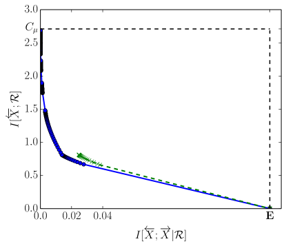
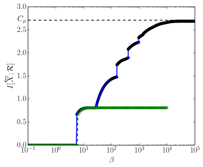
Figure 6: Simple Nonunifilar Source: (Top panel) Information function: coding cost versus distortion. (Bottom panel) Feature curve: coding cost as a function of inverse temperature $\beta$. (Blue solid line, circles) CIB with a $10$-state approximate $\epsilon$-machine. (Green dashed line, crosses) OCF at $M,N=1$.

Let’s test this intuition. The prototypical example with $\sigma_{\mu}(1)=0$ is the Golden Mean Process, whose HMM is shown in Fig. 5(top). It is order-$1$ Markov, so OCF with $L=1$ is provably equivalent to CIB, illustrating one side of the intuition.

A more discerning test is an infinite-order Markov process with small $\sigma_{\mu}$. One such process is the Simple Nonunifilar Source (SNS) whose (nonunifilar) HMM is shown in Fig. 5(bottom). As anticipated, Fig. 6(top) shows that OCF with $L=1$ and CIB yield very similar information functions at low code rate and low $\beta$. In fact, many of SNS’s statistics are well approximated by the Golden Mean HMM.

The feature curve in Fig. 6(bottom) reveals a slightly more nuanced story, however. The SNS is highly cryptic, in that it has a much larger $C_{\mu}$ than ${\bf E}$. As a result, OCF with $L=1$ approximates ${\bf E}$ quite well but underestimates $C_{\mu}$, replacing an (infinite) number of feature-discover transitions with a single transition. (More on these transitions shortly.i)

This particular type of error—missing predictive features—only matters for predicting the SNS when low distortion is desired. Nonetheless, it is important to remember that the process implied by OCF with $L=1$—the Golden Mean Process—is not the SNS. The Golden Mean Process is an order-$1$ Markov process. The SNS HMM is nonunifilar and generates an infinite-order Markov process and so provides a classic example [5] of how difficult it can be to exactly calculate information measures of stochastic processes.

Be aware that CIB cannot be directly applied to analyze the SNS, since the latter’s causal state space is countably infinite; see Ref. [63]’s Fig. 3. Instead, we used finite-time causal states with finite past and future lengths and with the state probability distribution given in App. B of Ref. [63]. Here, we used $M,N=10$, effectively approximating the SNS as an order-$10$ Markov process.

V.2 First-order Phase Transitions at $\beta=1$

Feature curves have discontinuous jumps (“first-order phase transitions”) or are nondifferentiable (“second-order phase transitions”) at critical temperatures when new features or new lossy causal states are discovered. The effective dimension of the codebook changes at these transitions. Symmetry breaking plays a key role in identifying the type and temperature of phase transitions in constrained optimization [19, 61]. Using the infinite-order Markov Even Process of Sec. III, CIB allows us to explore in greater detail why and when first-order phase transitions occur at $\beta=1$ in feature curves.

There are important qualitative differences between information functions and feature curves obtained via CIB and via OCF for the Even Process. First, as Fig. 7(top) shows, the Even Process CIB information function is a simple straight line, whereas those obtained from OCF are curved and substantially overestimate the code rate. Second, as Fig. 7(bottom) shows, the CIB feature curve is discontinuous at $\beta=1$, indicating a single first-order phase transition and the discovery of highly predictive states. In contrast, OCF functions miss that key transition and incorrectly suggest several phase transitions at larger $\beta$s.

The first result is notable, as Ref. [16] proposed that the curvature of OCF information functions define natural scales of predictive coarse-graining. In this interpretation, linear information functions imply that the Even Process has no such intermediate natural scales. And, there are good reasons for this.

So, why does the Even Process exhibit a straight line? Recall that the Even Process’s recurrent forward-time causal states code for whether or not one just saw an even number of $1$’s (state A) or an odd number of $1$’s (state B) since the last $0$. Its recurrent reverse-time causal states (Fig. 2 in Ref. [37]) capture whether or not one will see an even number of $1$’s until the next $0$ or an odd number of $1$’s until the next $0$. Since one only sees an even number of $1$’s between successive $0$’s, knowing the forward-time causal state uniquely determines the reverse-time causal state and vice versa. The Even Process’ forward causal-state distribution is $\Pr(\mathcal{S}^{+})=\big{(}2/3~{}1/3\big{)}$ and the conditional distribution of forward and reverse-time causal states is:

$$\Pr(\mathcal{S}^{-}|\mathcal{S}^{+})=\begin{pmatrix}1&0\\ 0&1\end{pmatrix}~{}.$$

Thus, there is an invertible transform between $\mathcal{S}^{+}$ and $\mathcal{S}^{-}$, a conclusion that follows directly from the process’s bidirectional machine. The result is that:

$$\operatorname{I}[\mathcal{R};\mathcal{S}^{+}]=\operatorname{I}[\mathcal{R};\mathcal{S}^{-}]~{}.$$ (17)

And so, we directly calculate the information function from Eq. (10):

$$R(I_{0}) =\min_{\operatorname{I}[\mathcal{R};\mathcal{S}^{-}]\geq I_{0}}\operatorname{I}[\mathcal{R};\mathcal{S}^{+}]$$

$$=\min_{\operatorname{I}[\mathcal{R};\mathcal{S}^{-}]\geq I_{0}}\operatorname{I}[\mathcal{R};\mathcal{S}^{-}]$$

$$=I_{0}~{},$$

for all $I_{0}\leq{\bf E}$. Similar arguments hold for periodic process as described in Ref. [15, 16] and for general cyclic (noisy periodic) processes as well. However, periodic processes are finite-order Markov, whereas the infinite Markov-order Even Process hides its deterministic relationship between prediction and retrodiction underneath a layer of stochasticity. This suggests that the bidirectional machine’s switching maps [37] are key to the shape of information functions.

The Even Process’s feature curve in (Fig. 7(bottom) shows a first-order phase transition at $\beta=1$. Similar to periodic and cyclic processes, its lossy causal states are all-or-nothing. Iterating Eqs. (14) and (16) is an attempt to maximize the objective function of Eq. (13). However, Eq. (17) gives:

$$\mathcal{L}_{\beta}=(1-\beta^{-1})\operatorname{I}[\mathcal{R};\mathcal{S}^{+}]~{}.$$

Recall that $0\leq\operatorname{I}[\mathcal{R};\mathcal{S}^{+}]\leq C_{\mu}$. For $\beta<1$, on the one hand, maximizing $\mathcal{L}_{\beta}$ requires minimizing $\operatorname{I}[\mathcal{R};\mathcal{S}^{+}]$, so the optimal lossy model is an i.i.d. approximation of the Even Process—a single-state HMM. For $\beta>1$, on the other, maximizing $\mathcal{L}_{\beta}$ requires maximizing $\operatorname{I}[\mathcal{R};\mathcal{S}^{+}]$, so the optimal lossy features are the causal states $A$ and $B$ themselves. At $\beta=1$, though, $\mathcal{L}_{\beta}=0$, and any representation $\mathcal{R}$ of the forward-time causal states $\mathcal{S}^{+}$ is optimal. In sum, the discontinuity of coding cost $\operatorname{I}[\mathcal{R};\mathcal{S}^{+}]$ as a function of $\beta$ corresponds to a first-order phase transition and the critical inverse temperature is $\beta=1$.

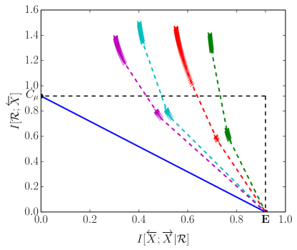
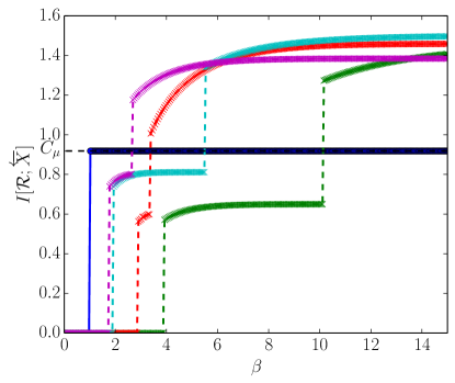
Figure 7: Even Process analyzed with CIB (solid line, blue circles) and with OCF (dashed lines, colored crosses) at various values of $M=N=L$: (right to left) $L=2$ (green), $L=3$ (red), $L=4$ (light blue), and $L=5$ (purple). (top) Information functions. (bottom) Feature curves. At $\beta=1$, CIB functions transition from approximating the Even Process as i.i.d. (biased coin flip) to identifying both causal states.

Both causal states in the Even Process are unusually predictive features: any increase in memory of such causal states is accompanied by a proportionate increase in predictive power. These states are associated with a one-to-one (switching) map between a forward-time and reverse-time causal state. In principle, such states should be the first features extracted by any PRD algorithm. More generally, when the joint probability distribution of forward- and reverse-time causal states can be permuted into diagonal block-matrix form, there should be a first-order phase transition at $\beta=1$ with one new codeword for each of the blocks.

Many processes do not have probability distributions over causal states that can be permuted, even approximately, into a diagonal block-matrix form; e.g., most of those described in Refs. [64, 63]. However, we suspect that diagonal block-matrix forms for $\Pr(\mathcal{S}^{+},\mathcal{S}^{-})$ might be relatively common in the highly structured processes generated by low-entropy rate deterministic chaos, as such systems often have many irreducible forbidden words. Restrictions on the support of the sequence distribution easily yields blocks in the joint probability distribution of forward- and reverse-time causal states.

For example, the Even Process forbids words with an odd number of $1$s, which is expressed by its irreducible forbidden word list $\mathcal{F}=\{01^{2k+1}0:k=0,1,2,\ldots\}$. Its causal states group pasts that end with an even (state $A$) or odd (state $B$) number of $1$s since the last $0$. Given the Even Process’ forbidden words $\mathcal{F}$, sequences following from state $A$ must start with an even number of ones before the next $0$ and those from state $B$ must start with an odd number of ones before the next $0$. The restricted support of the Even Process’ sequence distribution therefore gives its causal states substantial predictive power.

Moreover, many natural processes are produced by deterministic chaotic maps with added noise [65]. Such processes may also have $\Pr(\mathcal{S}^{+},\mathcal{S}^{-})$ in nearly diagonal block-matrix form. These joint probability distributions might be associated with sharp second-order phase transitions.

However, numerical results for the “four-blob” problem studied in Ref. [61] suggest the contrary. The joint probability distribution of compressed and relevant variables there has a nearly diagonal block-matrix form, with each block corresponding to one of the four blobs. If the joint probability distribution were exactly block diagonal—e.g., from a truncated mixture of Gaussians model—then the information function would be linear and the feature curve would exhibit a single first-order phase transition at $\beta=1$ from the above arguments. The information function for the four-blob problem looks linear; see Fig. $5$ of Ref. [61]. The feature curve (Fig. $4$, there) is entirely different from the feature curves that we would expect from our earlier analysis of the Even Process. Differences in the off-diagonal block-matrix structure allowed the annealing algorithm to discriminate between the nearly equivalent matrix blocks, so that there are three phase transitions to identify each of the four blobs. Moreover, none of the phase transitions are sharp. So, perhaps the sharpness of phase transitions in feature curves of noisy chaotic maps might have a singular noiseless limit, as is often true for information measures [64].

Figure 8: Random Insertion Process (RIP): (Top) Forward-time $\epsilon$-machine. (Bottom) Reverse-time $\epsilon$-machine.

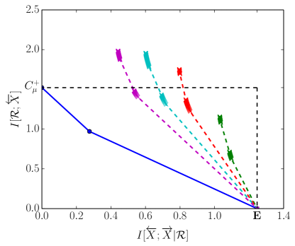
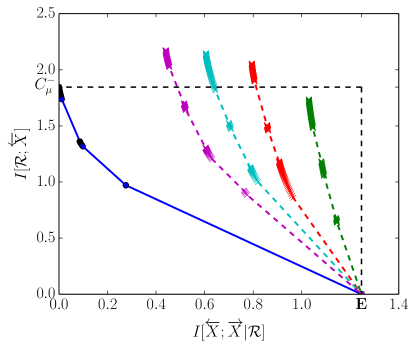
Figure 9: Random Insertion Process (RIP) Information Functions: RIP is a causally irreversible process: $C_{\mu}^{+}<C_{\mu}^{-}$. There are more causal states in reverse time than forward time, leading to more kinks in the reverse-time process’ information function (bottom) than in the forward-time process’ information function (top). Legend as in previous figure: (solid line, blue circles) CIB function and (dashed lines, colored crosses) OCF at various sequence lengths.

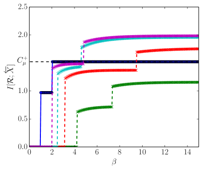
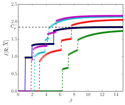
Figure 10: Random Insertion Process (RIP) Feature Curves: Having more causal states in reverse time than forward time leads to more phase transitions in the reverse-time process’ feature curve (bottom) than in the forward-time process’ feature curve (top). Legend as in previous figure.

V.3 Temporal Asymmetry in Lossy Prediction

As Refs. [35, 37] describe, the resources required to losslessly predict a process can change markedly under time reversal. The prototype example is the Random Insertion Process (RIP), shown in Fig.  8. Its bidirectional machine is known analytically [35]. Therefore, we know the joint $\Pr({\mathcal{S}}^{+},{\mathcal{S}}^{-})$ via $\Pr(\mathcal{S}^{+})=\big{(}2/5~{}1/5~{}2/5\big{)}$ and:

$$\Pr(\mathcal{S}^{-}|\mathcal{S}^{+})=\begin{pmatrix}0&\frac{1}{2}&0&\frac{1}{2}\\ 0&\frac{1}{2}&\frac{1}{2}&0\\ 1&0&0&0\end{pmatrix}~{}.$$

There are three forward-time causal states and four reverse-time causal states, and the forward-time statistical complexity and reverse-time statistical complexity are unequal, making the RIP causally irreversible. For instance, $C_{\mu}^{+}\approx 1.8$ bits and $C_{\mu}^{-}\approx 1.5$ bits, even though the excess entropy ${\bf E}\approx 1.24$ bits is by definition time-reversal invariant.

However, it could be that the lossy causal states are somehow more robust to time reversal than the (lossless) causal states themselves. Let’s investigate the difference in RIP’s information and feature curves under time reversal. Figure 9 shows information functions for the forward-time and reverse-time processes. Despite RIP’s causal irreversibility, information functions look similar until informational distortions of less than $0.1$ bits. RIP’s temporal correlations are sufficiently long-ranged so as to put OCF with $L\leq 5$ at a significant disadvantage relative to CIB, as the differences in the information functions demonstrate. OCF greatly underestimates ${\bf E}$ by about $30\%$ and both underestimates and overestimates the correct $C_{\mu}$.

The RIP feature curves in Fig. 10 reveal a similar story in that OCF fails to asymptote to the correct $C_{\mu}$ for any $L\leq 5$ in either forward or reverse time. Unlike the information functions, though, feature curves reveal temporal asymmetry in the RIP even in the lossy (low $\beta$) regime.

Both forward and reverse-time feature curves show a first-order phase transition at $\beta=1$, at which point the forward-time causal state $C$ and the reverse-time causal state $D$ are added to the codebook, illustrating the argument of Sec. V.2. (Forward-time causal state $C$ and reverse-time causal state $D$ are equivalent to the same bidirectional causal state $C/D$ in RIP’s bidirectional $\epsilon$-machine. See Fig. 2 of Ref. [35].) This common bidirectional causal state is the main source of similarity in the information functions of Fig. 9.

Both feature curves also show phase transitions at $\beta=2$, but similarities end there. The forward-time feature curve shows a first-order phase transition at $\beta=2$, at which point both remaining forward-time causal states $A$ and $B$ are added to the codebook. The reverse-time feature curve has what looks to be a sharp second-order phase transition at $\beta=2$, at which point the reverse-time causal state $F$ is added to the codebook. The remaining two reverse-time causal states, $E$ and $G$, are finally added to the codebook at $\beta=5$. We leave solving for the critical temperatures and confirming the phase transition order using a bifurcation discriminator [59] to the future.

V.4 Predictive Hierarchy in a Dynamical System

Up to this point, the emphasis was analyzing selected prototype infinite Markov-order processes to illustrate the differences between CIB and OCF. In the following, instead we apply CIB and OCF to gain insight into a nominally more complicated process—a one-dimensional chaotic map of the unit interval—in which we emphasize the predictive features detected. We consider the symbolic dynamics of the Tent Map at the Misiurewicz parameter $a=\big{(}\sqrt[3]{9+\sqrt{57}}+\sqrt[3]{9-\sqrt{57}}\big{)}3^{-\frac{2}{3}}$, studied in Ref. [66]. Figure 11 gives both the Tent Map and the analytically derived $\epsilon$-machine for its symbolic dynamics, from there. The latter reveals that the symbolic dynamic process is infinite-order Markov. The bidirectional $\epsilon$-machine at this parameter setting is also known. Hence, one can directly calculate information functions as described in Sec. V.

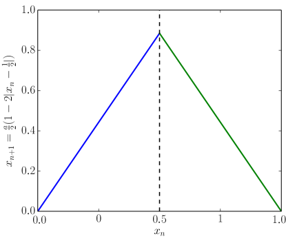
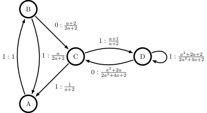
Figure 11: Symbolic dynamics of the Tent Map at the Misiurewicz parameter $a$. (top) The map iterates points $x_{n}$ in the unit interval $[0,1]$ according to $x_{n+1}=\frac{a}{2}(1-2|x_{n}-\frac{1}{2}|)$, with $x_{0}\in[0,1]$. The symbolic dynamics translates the sequence $x_{0},x_{1},x_{2},\ldots$ of real values to a $0$ when $x_{n}\in[0,\frac{1}{2})$ and to a $1$ when $x_{n}\in[\frac{1}{2},1]$. (bottom) Calculations described elsewhere [66] yield the $\epsilon$-machine shown. (Reproduced from Ref. [66] with permission.)

From Fig. 12’s information functions, one easily gleans natural coarse-grainings, scales at which there is new structure, from the functions’ steep regions. As is typically true, the steepest part of the predictive information function is found at very low rates and high distortions. Though the information function of Fig. 12(top) is fairly smooth, the feature curve (Fig. 12(bottom)) reveals phase transitions where the feature space expands a lossier causal state into two distinct representations.

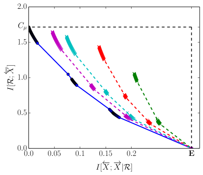
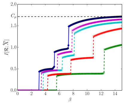
Figure 12: Rate distortion analysis for symbolic dynamics of the Tent Map at the Misiurewicz parameter $a$ given in the text. (top) Information functions. (bottom) Feature curves. Comparing CIB (solid line, blue circles) and OCF (dashed lines, colored crosses) at several values of $L$. Legend same as previous.

(a)
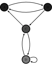
(b)
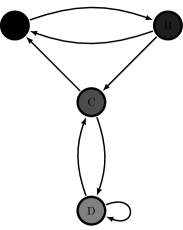
(c)
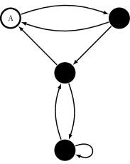
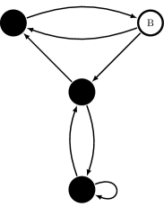
(d)

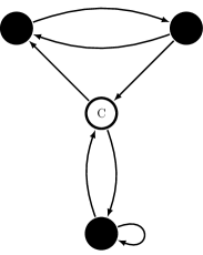
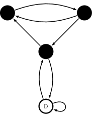
Figure 13: Tent Map predictive features as a function of inverse temperature $\beta$: Each state-transition diagram shows the $\epsilon$-machine in Fig. 11(bottom) with nodes gray-scaled by $\Pr(\mathcal{S}^{+}|\mathcal{R}=r)$ for each $r\in\mathcal{R}$. White denotes high probability and black low. Transitions are shown only to guide the eye. (a) $\beta=0.01$: one state that puts unequal weights on states $C$ and $D$. (b) $\beta=1.9$: two states identified, $A$ and a mixture of $C$ and $D$. (c) $\beta=3.1$: three states are identified, $A$, $B$, and the mixture of $C$ and $D$. (d) $\beta\to\infty$: original four states identified, $A$, $B$, $C$, and $D$.

To appreciate the changes in underlying predictive features as a function of inverse temperature, Fig. 13 shows the probability distribution $\Pr(\mathcal{S}^{+}|\mathcal{R})$ over causal states given each compressed variable—the features. What we learn from such phase transitions is that some causal states are more important than others and that the most important ones are not necessarily intuitive. As we move from lossy to lossless ($\beta\to\infty$) predictive features, we add forward-time causal states to the representation in the order $A$, $B$, $C$, and finally $D$. The implication is that $A$ is more predictive than $B$, which is more predictive than $C$, which is more predictive than $D$. Note that this predictive hierarchy is not the same as a “stochastic hierarchy” in which one prefers causal states with smaller $\operatorname{H}[{X}_{0}|\mathcal{S}^{+}=\sigma^{+}]$. The latter is equivalent to an ordering based on correctly predicting only one time step into the future. Such a hierarchy privileges causal state $C$ over $B$ based on the transition probabilities shown in Fig. 11(bottom), in contrast to how CIB orders them.

VI Computational Challenges

Proposition 1 and Thm. 1 says that one can calculate PRD functions (including PIB functions) in three steps:

1. Theoretically derive a system’s $\epsilon$-machine [5, 67] using Eq. (3) or empirically estimate an $\epsilon$-machine [68, 69, 70, 71, 15, 72, 48];

2. Calculate the joint probability distribution over forward- and reverse-time causal states [5, 35, 37]; and

3. Apply a rate-distortion algorithm to compress $\mathcal{S}^{+}$ to minimize expected distortion about $\mathcal{S}^{-}$ for a desired distortion.

From the computational complexity viewpoint [73] each step is hard.

Recall that NP refers to the class of decision problems for which a deterministic Turing machine can verify a “yes” answer in polynomial-time; an NP-hard problem is one that is as hard as the hardest problems in NP. Such problems are quite familiar. Many computations related to spin glass Ising models are NP-hard [74]. Inferring an $\epsilon$-machine from samples is very likely NP-hard, given the computational complexity hardness results on passively inferring nonprobabilistic finite automata from only positive examples [75, and citations therein]. Calculating $\Pr({\mathcal{S}}^{+},{\mathcal{S}}^{-})$ from an $\epsilon$-machine typically has run time and storage requirements exponential in $|{\mathcal{S}}^{+}|$. Solving the associated PRD optimization is known to be NP-hard [76].

It may seem as though the three-step approach is overly complicated, especially when compared to the more common approach in which one directly clusters finite-length pasts to retain information about finite-length futures. In point of fact, algorithms based on clustering pasts and futures of length $L$ themselves cannot avoid the basic complexities, either. Rather, they implicitly assume that an order-$L$ Markov model of the underlying process is sufficiently predictive for calculating information functions. When this assumption fails—which happens often, as Sec. III explained—then algorithms that explicitly cluster sequences produce suboptimal results. Recall the examples in Sec. V. In short, clustering in sequence distribution space without first inferring a model leaves one unwittingly prone to the detrimental effects model mismatch—using sequence histograms rather than $\epsilon$-machines. Building predictive models first was also found to be particularly effective when estimating a process’s large deviations [77].

VII Conclusion

We introduced a new relationship between predictive rate-distortion and causal states. Theorem $1$ of Refs. [15, 16] say that the predictive information bottleneck can identify forward-time causal states, in theory. The analyses and results in Secs. III-V suggest that in practice, when studying time series with longer-range temporal correlations, we calculate substantially more accurate predictive information functions by deriving or inferring an approximate $\epsilon$-machine first.

The culprit is the curse of dimensionality for prediction: the number of possible sequences increases exponentially with their length. The longer-ranged the temporal correlations, the longer sequences need to be. And, as Sec. III demonstrated, a process need not have very long-ranged temporal correlations for the curse of dimensionality to rear its head.

Section V.1 showed that building a model may be unnecessary if the underlying process effectively has small, finite Markov order, since sequences are adequate proxies for a process’s effective states. Sections V.2-V.4, however, then showed that when the underlying process has long-range temporal correlations—either larger Markov order than sequence lengths used or infinite Markov order—then computing PRD functions directly from sequence distributions produces quantitatively inaccurate and structurally misleading results. Since an exhaustive survey [39] shows that infinite Markov order dominates the space of processes generated by even finite HMMs, these problems are likely generic and could very well have affected a number of existing calculations of rate-distortion functions, calling into question derived interpretations.

Figure 14: Prescient models and inferring information properties: Estimating information measures directly from sequence data encounters a curse of dimensionality or, in other words, severe undersampling. Instead, one can calculate information measures in closed-form from (derived or inferred) maximally predictive (prescient) models [53]. Rate-distortion functions are now on the list of information properties that can be accurately calculated. Alternate generative models that are not prescient cannot be used directly, as Blackwell showed in the 1950s [78].

On the one hand, with these thoughts in mind, our results can be interpreted as a cautionary tale about the curse of dimensionality inherent in predictive rate-distortion. On the other hand, quantifying that curse of dimensionality fully in Sec. V suggested new algorithms for accurately and efficiently calculating information functions and feature curves. Figure 14 highlights the two sides of this coin and the alternative strategies that were compared.

These lessons echo that found when analyzing a process’s large deviations [77]: Estimate a predictive model first and use it to estimate the probability of extreme events, events that almost by definition are not in the original data used for model inference. There may be applications that only need temporally local predictive feature extraction—e.g., that in Ref. [10]—and, then, by assumption there is no such curse of dimensionality. Even then, one often assumes that temporally local learning rules will yield temporally long-ranged predictive features. In this situation, causal rate distortion could provide benchmarks for testing the performance of temporally local predictive feature extractors on infinite-order Markov processes.

The relationship between predictive rate-distortion and causal states runs much deeper than we probed here. At a minimum, CRD is a useful theoretical tool for analyzing coarse-grained features. One technical aspect appeared in our discussion of how the bidirectional machine’s switching maps determine much of an information function’s shape. Perhaps more importantly, though, the predictive features identified using these methods are statistics and not full machines with both a state space and dynamic [49]. (Although one can certainly build lossy machines from these predictive features they are likely to be nonunifilar and not even generate the given process.) Inferring lossy predictive machines requires a different approach, such as the recursive information bottleneck [48]. Reformulating that objective function in terms of the bidirectional machine is an important avenue of future research. Success in developing this will prove useful in sensorimotor loop applications, where one learns predictive models actively rather than passively [79, 12, 14, 13].

Section IV’s methods can be directly extended to completely different rate-distortion settings, such as when the underlying minimal directed acyclic graphical model between compressed and relevant random variables is arbitrarily large and highly redundant. Also, despite the restrictions that Prop. 1 places on the distortion measures for which CRD and PRD are equivalent, the discussion in App. A suggests that CRD can be used instead of PRD if one correctly modifies the distortion measure. This opens up a wide range of applications; for example, those in which other properties, besides structure or prediction, are desired, such as optimizing utility functions.

Finally, one immediate application—the construction of a predictive hierarchy—was suggested in Sec. V.4, using the stochastic process defined by symbolic dynamics of a chaotic dynamical system. We saw that rate-distortion analysis provided a principled way to determine which temporal or spatial structures are emergent. In other words, CIB is a new tool for accurately identifying emergent macrostates of a stochastic process [5]. Used in this way, CIB becomes a tool relevant to biological, neurobiological, and social science phenomena in which the key emergent features are not known a priori or from first-principles calculation. In the context of neurobiological data, for example, such macrostates can provide approximately predictive models of neural spike trains; e.g., see Ref. [80]. In the context of social science data, they might be related to new kinds of community organization. While it is encouraging to look forward, we appreciate that natural processes are quite complicated and that there is quite a way to go before we have fully automated detection of emergent macrostates.

Appendix A Causal Rate-Distortion Proofs

We assume familiarity with rate-distortion theory on the level of Refs. [27, Ch. 8] and [42].

We designed the proofs to be as elementary as possible; they are basically repeated applications of the Markov loop in Fig. 1 and the pullback method from probability theory. They are also in effect sketches more than they are proofs. This allows us to highlight their construction nature. All statements can almost be proven through repeated applications of the Markov loop in Fig. 1 to the formal solution for optimal stochastic codebooks given by Theorem $4$ of Ref. [44]. The “almost” comes from the fact that not all solutions to the original rate-distortion objective function maximize the annealing objective function [61].

Theorem 1 does not necessarily mean that the solutions to the annealing objectives of PIB and CIB are the same. Rather, it only finds equivalence between solutions to the original rate distortion optimizations. However, the same arguments straightforwardly imply that the annealing objective functions associated with PIB and CIB also have equivalent solutions.

We consider two types of information sources and corresponding encoders. For one, the input information source is $\smash{\overleftarrow{{X}}}$—the process in question—with sample space $\smash{\overleftarrow{{\rm{\bf{X}}}}}$. Its associated codebook is denoted by $\mathcal{R}$ with sample space $\smash{\overleftarrow{{\rm{\bf{X}}}}}$. (The sample space is specified for concreteness, though unnecessary in general.) And, the distortion measure is $d:\smash{\overleftarrow{{\rm{\bf{X}}}}}\times\smash{\overleftarrow{{\rm{\bf{X}}}}}\rightarrow\Re^{+}$.

For the other, the input information source is $\mathcal{S}^{+}$—the internal causal-state process—with sample space $\epsilon^{+}(\smash{\overleftarrow{{\rm{\bf{X}}}}})$ determined by the causal-state map; see Ref. [2]. Its codebook is denoted $\widehat{\mathcal{R}}$ with sample space $\epsilon^{+}\big{(}\smash{\overleftarrow{{\rm{\bf{X}}}}}\big{)}$. (Again, this is for concreteness, but unnecessary in general.) And, its distortion measure is $\widehat{d}:\epsilon^{+}\big{(}\smash{\overleftarrow{{\rm{\bf{X}}}}}\big{)}\times\epsilon^{+}\big{(}\smash{\overleftarrow{{\rm{\bf{X}}}}}\big{)}\rightarrow\Re^{+}$.

Implicitly, by specifying that our codebooks produce codewords in the same sample space of the inputs themselves, we combine the encoder and decoder of Fig. 2(top) into a single information processing unit.

Using the fact that the two source sample spaces and codebooks are intimately related via the causal-state map $\sigma^{+}=\epsilon^{+}({\smash{\overleftarrow{{x}}}})$, we construct codebooks in one sample space out of codebooks from the other. For instance, a given process codebook $\mathcal{R}$ implies a causal-state codebook $\mathcal{R}_{\epsilon^{+}}$ with realizations $r_{\epsilon^{+}}\in\epsilon^{+}(\smash{\overleftarrow{{\rm{\bf{X}}}}})$:

$$\Pr(\mathcal{R}_{\epsilon^{+}}|\mathcal{S}^{+}=\sigma^{+})$$

$$=\sum_{{\smash{\overleftarrow{{x}}}}\in\smash{\overleftarrow{{\rm{\bf{X}}}}}}\Pr\big{(}\mathcal{R}_{\epsilon^{+}}|\smash{\overleftarrow{{X}}}={\smash{\overleftarrow{{x}}}},\mathcal{S}^{+}=\sigma^{+}\big{)}\Pr\big{(}\smash{\overleftarrow{{X}}}={\smash{\overleftarrow{{x}}}}|\mathcal{S}^{+}=\sigma^{+}\big{)}$$

$$=\sum_{{\smash{\overleftarrow{{x}}}}:\epsilon^{+}({\smash{\overleftarrow{{x}}}})=\sigma^{+}}\Pr\big{(}\mathcal{R}|\smash{\overleftarrow{{X}}}={\smash{\overleftarrow{{x}}}}\big{)}\Pr\big{(}\smash{\overleftarrow{{X}}}={\smash{\overleftarrow{{x}}}}\big{)}~{}.$$

This is essentially the pullback method of probability theory. Similarly, a given causal-state codebook $\widehat{\mathcal{R}}$ can be naturally extended to a process codebook $\widehat{\mathcal{R}}_{{\smash{\overleftarrow{{x}}}}}$ with realizations $\widehat{r}_{{\smash{\overleftarrow{{x}}}}}\in\smash{\overleftarrow{{\rm{\bf{X}}}}}$:

$$\Pr\big{(}\widehat{\mathcal{R}}_{{\smash{\overleftarrow{{x}}}}}|\smash{\overleftarrow{{X}}}={\smash{\overleftarrow{{x}}}}\big{)} =\Pr\big{(}\widehat{\mathcal{R}}|\mathcal{S}^{+}=\epsilon^{+}({\smash{\overleftarrow{{x}}}})\big{)}~{}.$$

In this way, we compare $\widehat{\mathcal{R}}$ to $\mathcal{R}$, using $\widehat{\mathcal{R}}_{{\smash{\overleftarrow{{x}}}}}$. To simplify these comparisons, if $\mathcal{Q}$ is some codebook, in the following $\mathcal{Q}_{\epsilon^{+}}$ and $(\mathcal{Q})_{\epsilon^{+}}$ denote a codebook over causal states and $\mathcal{Q}_{{\smash{\overleftarrow{{x}}}}}$ and $(\mathcal{Q})_{{\smash{\overleftarrow{{x}}}}}$ a codebook over process pasts.

Here, we only consider distortion measures of the form:

$$d({\smash{\overleftarrow{{x}}}},r) =f\big{(}\Pr(\smash{\overrightarrow{{X}}}|\smash{\overleftarrow{{X}}}={\smash{\overleftarrow{{x}}}}),\Pr(\smash{\overrightarrow{{X}}}|\mathcal{R}=r)\big{)}$$

and

$$\widehat{d}(\sigma^{+},\widehat{r}) =f\big{(}\Pr(\smash{\overrightarrow{{X}}}|\mathcal{S}^{+}=\sigma^{+}),\Pr(\smash{\overrightarrow{{X}}}|\widehat{\mathcal{R}}=\widehat{r})\big{)}~{},$$

for some unspecified $f(\cdot,\cdot)$ that quantifies differences between probability distributions; e.g., Kullback-Liebler or Shannon-Jensen divergence. Causal shielding implies that:

$$\Pr(\smash{\overrightarrow{{X}}}|\smash{\overleftarrow{{X}}}={\smash{\overleftarrow{{x}}}})=\Pr(\smash{\overrightarrow{{X}}}|\mathcal{S}^{+}=\epsilon^{+}({\smash{\overleftarrow{{x}}}}))$$

and:

$$\Pr(\smash{\overrightarrow{{X}}}|\mathcal{R}) =\sum_{\sigma^{+}\in\bm{\mathcal{S}}^{+}}\Pr(\smash{\overrightarrow{{X}}}|\mathcal{S}^{+}=\sigma^{+})\Pr(\mathcal{S}^{+}=\sigma^{+}|\mathcal{R})$$

$$=\sum_{\sigma^{+}\in\bm{\mathcal{S}}^{+}}\Pr(\smash{\overrightarrow{{X}}}|\mathcal{S}^{+}=\sigma^{+})\Pr(\mathcal{S}^{+}=\sigma^{+}|\mathcal{R}_{\epsilon^{+}})~{}.$$

By construction, then:

$$d({\smash{\overleftarrow{{x}}}},r)=\widehat{d}(\epsilon^{+}({\smash{\overleftarrow{{x}}}}),r_{\epsilon^{+}})$$

and

$$\widehat{d}(\sigma^{+},\widehat{r})=d({\smash{\overleftarrow{{x}}}},\widehat{r}_{{\smash{\overleftarrow{{x}}}}})~{},$$

for all ${\smash{\overleftarrow{{x}}}}$ such that $\epsilon^{+}({\smash{\overleftarrow{{x}}}})=\sigma^{+}$.

On the one hand, when the information source is $\smash{\overleftarrow{{X}}}$, we consider the following rate-distortion function:

$$R(D) =\min_{\langle d({\smash{\overleftarrow{{x}}}},r)\rangle_{\mathcal{R},\smash{\overleftarrow{{X}}}}\leq D}\operatorname{I}[\mathcal{R};\smash{\overleftarrow{{X}}}]$$

and its associated optimal codebook:

$$\mathcal{R}^{*}_{D} =\operatorname*{argmin}_{\langle d({\smash{\overleftarrow{{x}}}},r)\rangle_{\mathcal{R},\smash{\overleftarrow{{X}}}}\leq D}\operatorname{I}[\mathcal{R};\smash{\overleftarrow{{X}}}]~{}.$$

On the other, when the information source is $\mathcal{S}^{+}$, we consider the following rate-distortion function:

$$\widehat{R}(D) =\min_{\langle\widehat{d}(\sigma^{+},\widehat{r})\rangle_{\widehat{\mathcal{R}},\mathcal{S}^{+}}\leq D}\operatorname{I}[\widehat{\mathcal{R}};\mathcal{S}^{+}]$$

and its associated optimal codebook:

$$\widehat{\mathcal{R}}^{*}_{D} =\operatorname*{argmin}_{\langle\widehat{d}(\sigma^{+},\widehat{r})\rangle_{\widehat{\mathcal{R}},\mathcal{S}^{+}}\leq D}\operatorname{I}[\widehat{\mathcal{R}};\mathcal{S}^{+}]~{}.$$ (18)

The lemma below, a more precise version of the main text’s Lemma 1, states their relationship.

Lemma 1. $R(D)=\widehat{R}(D)$ and $\mathcal{R}^{*}_{D}\simeq\widehat{\mathcal{R}}^{*}_{D}$ for all achievable $D$.

Proof.

First, to establish the isomorphism we construct a map between the process and causal-state codebooks, showing that $\mathcal{R}^{*}_{D}=((\mathcal{R}_{\epsilon^{+}})^{*}_{D})_{{\smash{\overleftarrow{{x}}}}}$ via a proof by contradiction. Suppose they are not equal. As described earlier:

$$D =\big{\langle}d({\smash{\overleftarrow{{x}}}},r)\big{\rangle}_{\mathcal{R}^{*}_{D},\smash{\overleftarrow{{X}}}}$$

$$=\big{\langle}\widehat{d}(\sigma^{+},r_{\epsilon^{+}})\big{\rangle}_{(\mathcal{R}_{\epsilon^{+}})^{*}_{D},\mathcal{S}^{+}}$$

$$=\big{\langle}d({\smash{\overleftarrow{{x}}}},(r_{\epsilon^{+}})_{{\smash{\overleftarrow{{x}}}}})\big{\rangle}_{((\mathcal{R}_{\epsilon^{+}})^{*}_{D})_{{\smash{\overleftarrow{{x}}}}},\smash{\overleftarrow{{X}}}}~{}.$$

So, the two codebook random variables have the same expected distortion. Since $\mathcal{R}^{*}_{D}\neq((\mathcal{R}_{\epsilon^{+}})^{*}_{D})_{{\smash{\overleftarrow{{x}}}}}$, $\Pr(\mathcal{R}^{*}_{D},\smash{\overleftarrow{{X}}}|\mathcal{S}^{+})\neq\Pr(\mathcal{R}^{*}_{D}|\mathcal{S}^{+})\Pr(\smash{\overleftarrow{{X}}}|\mathcal{S}^{+})$ and thus $\operatorname{I}[\mathcal{R}^{*}_{D};\smash{\overleftarrow{{X}}}|\mathcal{S}^{+}]>0$. This implies that $((\mathcal{R}_{\epsilon^{+}})^{*})_{\smash{\overleftarrow{{x}}}}$ has a lower coding cost:

$$\operatorname{I}[\mathcal{R}^{*}_{D};\smash{\overleftarrow{{X}}}] =\operatorname{I}[\mathcal{R}^{*}_{D};\mathcal{S}^{+}]+\operatorname{I}[\mathcal{R}^{*}_{D};\smash{\overleftarrow{{X}}}|\mathcal{S}^{+}]$$

$$>\operatorname{I}[\mathcal{R}^{*}_{D};\mathcal{S}^{+}]$$

$$=\operatorname{I}[(\mathcal{R}_{\epsilon^{+}})^{*}_{D};\mathcal{S}^{+}]$$

$$=\operatorname{I}[((\mathcal{R}_{\epsilon^{+}})^{*}_{D})_{\smash{\overleftarrow{{x}}}};\mathcal{S}^{+}]~{}.$$

Since $((\mathcal{R}_{\epsilon^{+}})^{*}_{D})_{\smash{\overleftarrow{{x}}}}$ is a codebook with the same expected distortion as $\mathcal{R}^{*}_{D}$ and lower coding cost, our assumption that they are not equal is incorrect and so $\mathcal{R}^{*}_{D}=((\mathcal{R}_{\epsilon^{+}})^{*}_{D})_{\smash{\overleftarrow{{x}}}}$.

Second, to show that $(\widehat{\mathcal{R}}_{{\smash{\overleftarrow{{x}}}}})^{*}_{D}=\mathcal{R}^{*}_{D}$, we only need to show that $(\widehat{\mathcal{R}}_{{\smash{\overleftarrow{{x}}}}})^{*}_{D}=(\mathcal{R}_{\epsilon^{+}})^{*}_{D}$ since the extension from codebooks $\widehat{\mathcal{R}}$ to codebooks $\mathcal{R}$ is injective. The reduced codebook $(\mathcal{R}_{\epsilon^{+}})^{*}_{D}$ inherits a constraint:

$$\langle d({\smash{\overleftarrow{{x}}}},r)\rangle_{\mathcal{R}^{*}_{D},\smash{\overleftarrow{{X}}}}=\langle\widehat{d}(\sigma^{+},r_{\epsilon^{+}})\rangle_{(\mathcal{R}_{\epsilon^{+}})^{*}_{D},\mathcal{S}^{+}}\leq D$$

and must minimize coding cost $\operatorname{I}[\mathcal{R}^{*}_{D};\smash{\overleftarrow{{X}}}]=\operatorname{I}[(\mathcal{R}_{\epsilon^{+}})^{*}_{D};\mathcal{S}^{+}]$, as described above. In short, $(\mathcal{R}_{\epsilon^{+}})^{*}_{D}$ satisfies:

$$(\mathcal{R}_{\epsilon^{+}})^{*}_{D} =\operatorname*{argmin}_{\langle\widehat{d}(\sigma^{+},r_{\epsilon^{+}})\rangle_{(\mathcal{R}_{\epsilon^{+}})^{*}_{D},\mathcal{S}^{+}}\leq D}\operatorname{I}[(\mathcal{R}_{\epsilon^{+}})^{*}_{D};\mathcal{S}^{+}]~{}.$$ (19)

Comparing Eq. (18) to Eq. (19) yields:

$$\widehat{\mathcal{R}}^{*}_{D} =(\mathcal{R}_{\epsilon^{+}})^{*}_{D}$$

$$(\widehat{\mathcal{R}}^{*}_{D})_{\smash{\overleftarrow{{x}}}} =((\mathcal{R}_{\epsilon^{+}})^{*}_{D})_{\smash{\overleftarrow{{x}}}}$$

$$=\mathcal{R}^{*}_{D}~{},$$

as desired. Using earlier manipulations, we also see that:

$$R(D) =\operatorname{I}[\mathcal{R}^{*}_{D};\smash{\overleftarrow{{X}}}]$$

$$=\operatorname{I}[(\mathcal{R}_{\epsilon^{+}})^{*}_{D};\mathcal{S}^{+}]$$

$$=\operatorname{I}[\widehat{\mathcal{R}}^{*}_{D};\mathcal{S}^{+}]$$

$$=\widehat{R}(D)~{}.$$

completing the proof sketch.

Next, consider an alternate class of causal-state codebooks $\widetilde{\mathcal{R}}$ and realizations $\widetilde{r}$ for coding information sources $\mathcal{S}^{+}$. These are distinguished by a new distortion measure:

$$\widetilde{d}(\sigma^{+},\widetilde{r})=f\big{(}\Pr(\mathcal{S}^{-}|\mathcal{S}^{+}=\sigma^{+}),\Pr(\mathcal{S}^{-}|\widetilde{\mathcal{R}}=\widetilde{r})\big{)}~{}.$$

The associated rate-distortion function is:

$$\widetilde{R}(D)=\min_{\langle\widetilde{d}(\sigma^{+},\widetilde{r})\rangle_{\widetilde{\mathcal{R}},\mathcal{S}^{+}}\leq D}\operatorname{I}[\widetilde{\mathcal{R}};\mathcal{S}^{+}]~{},$$

with optimal codebooks:

$$\widetilde{\mathcal{R}}^{*}_{D}=\operatorname*{argmin}_{\langle\widetilde{d}(\sigma^{+},\widetilde{r})\rangle_{\widetilde{\mathcal{R}},\mathcal{S}^{+}}\leq D}\operatorname{I}[\widetilde{\mathcal{R}};\mathcal{S}^{+}]~{}.$$ (20)

We would like to know the relationship between $R(D)$ and $\widetilde{R}(D)$, among other things. The proposition below, a more precise version of the main text’s Prop. 1, states their relationship.

Proposition 1. $R(D)=\widetilde{R}(D)$ and $(\widetilde{\mathcal{R}}^{*}_{D})_{\smash{\overleftarrow{{x}}}}=\mathcal{R}^{*}_{D}$ for all achievable $D$ if:

$$f\big{(}\Pr(\smash{\overrightarrow{{X}}} |\mathcal{S}^{+}=\sigma^{+}),\Pr(\smash{\overrightarrow{{X}}}|\widetilde{\mathcal{R}}=\widetilde{r})\big{)}$$

$$=f\big{(}\Pr(\mathcal{S}^{-}|\mathcal{S}^{+}=\sigma^{+}),\Pr(\mathcal{S}^{-}|\widetilde{\mathcal{R}}=\widetilde{r})\big{)}~{}.$$

Proof.

Given the condition, $\widehat{d}(\sigma^{+},\widetilde{r})=\widetilde{d}(\sigma^{+},\widetilde{r})$ and $\widehat{d}$ and $\tilde{d}$ are equivalent distortion measures. Then $\widehat{\mathcal{R}}^{*}_{D}=\widetilde{\mathcal{R}}^{*}_{D}$ and $\widehat{R}(D)=\widetilde{R}(D)$. The conclusion follows from Lemma 1 above.

There are many distortion measures that do not satisfy the constraints in Prop. 1. As an example, we focus on mean squared error and still can use the Markov chains $\mathcal{R}\rightarrow\mathcal{S}^{-}\rightarrow\smash{\overrightarrow{{X}}}$ and $\smash{\overleftarrow{{X}}}\rightarrow\mathcal{S}^{-}\rightarrow\smash{\overrightarrow{{X}}}$ to some benefit:

$$d({\smash{\overleftarrow{{x}}}},r) = \sum_{\smash{\overrightarrow{{x}}}}\left(\Pr(\smash{\overrightarrow{{X}}}=\smash{\overrightarrow{{x}}}|\smash{\overleftarrow{{X}}}={\smash{\overleftarrow{{x}}}})-\Pr(\smash{\overrightarrow{{X}}}=\smash{\overrightarrow{{x}}}|\mathcal{R}=r)\right)^{2}$$ (21)

$$= \sum_{\sigma^{-}}\left(\sum_{\smash{\overrightarrow{{x}}}\in\epsilon^{-}(\sigma^{-})}\Pr(\smash{\overrightarrow{{X}}}=\smash{\overrightarrow{{x}}}|\mathcal{S}^{-}=\sigma^{-})^{2}\right)\left(\Pr(\mathcal{S}^{-}=\sigma^{-}|\smash{\overleftarrow{{X}}}={\smash{\overleftarrow{{x}}}})-\Pr(\mathcal{S}^{-}=\sigma^{-}|\mathcal{R}=r)\right)^{2}.$$ (22)

Here, each reverse-time causal state is associated with a weighting factor:

$$\sum_{\smash{\overrightarrow{{x}}}\in\epsilon^{-}(\sigma^{-})}\Pr(\smash{\overrightarrow{{X}}}=\smash{\overrightarrow{{x}}}|\mathcal{S}^{-}=\sigma^{-})^{2}~{}.$$

This weighting factor typically vanishes if the futures are semi-infinite, since:

$$\sum_{\smash{\overrightarrow{{x}}}\in\epsilon^{-}(\sigma^{-})}\Pr(\smash{\overrightarrow{{X}}}=\smash{\overrightarrow{{x}}}|\mathcal{S}^{-}=\sigma^{-})=1$$

and $0\leq\Pr(\smash{\overrightarrow{{X}}}=\smash{\overrightarrow{{x}}}|\mathcal{S}^{-}=\sigma^{-})$. This issue is easily addressed by rescaling the weighting factor for finite-length futures by an appropriate function of the length and then taking the limit of this rescaled weighting factor as the length tends to infinity.

So, again, distortion measures that do not satisfy Prop. 1’s conditions implicitly privilege one reverse-time causal state over another.

Finally, we concentrate on a particularly useful distortion measure that satisfies the above constraint. OCI compresses $\smash{\overleftarrow{{X}}}$ to retain information about $\smash{\overrightarrow{{X}}}$, resulting in the information function:

$$R(I_{0}) =\min_{\operatorname{I}[\mathcal{R};\smash{\overrightarrow{{X}}}]\geq I_{0}}\operatorname{I}[\smash{\overleftarrow{{X}}};\mathcal{R}]$$

and the associated representation is:

$$\mathcal{R}^{*}_{I_{0}} =\operatorname*{argmin}_{\operatorname{I}[\mathcal{R};\smash{\overrightarrow{{X}}}]\geq I_{0}}\operatorname{I}[\smash{\overleftarrow{{X}}};\mathcal{R}]~{}.$$

In contrast, CIB, using causal states as proxies for the past and future, compresses $\mathcal{S}^{+}$ to retain information about $\mathcal{S}^{-}$, yielding the information function:

$$\widetilde{R}(I_{0}) =\min_{\operatorname{I}[\widetilde{\mathcal{R}};\mathcal{S}^{-}]\geq I_{0}}\operatorname{I}[\mathcal{S}^{+};\widetilde{\mathcal{R}}]~{},$$

with associated representations:

$$\widetilde{\mathcal{R}}^{*}_{I_{0}} =\operatorname*{argmin}_{\operatorname{I}[\widetilde{\mathcal{R}};\mathcal{S}^{-}]\geq I_{0}}\operatorname{I}[\mathcal{S}^{+};\widetilde{\mathcal{R}}]~{}.$$

OCI maximizes information about the future, whereas PRD minimizes distortion of predictions of the future. To emphasize the difference, we replaced $D$ with $I_{0}$, following Ref. [61].

Theorem 1. $R(I_{0})=\widetilde{R}(I_{0})$ and $(\widetilde{\mathcal{R}}^{*}_{I_{0}})_{\smash{\overleftarrow{{x}}}}=\mathcal{R}^{*}_{I_{0}}$ for all achievable $I_{0}$.

Proof.

First, consider PRD with distortion measure $d({\smash{\overleftarrow{{x}}}},r)={D_{\textrm{KL}}}[\Pr(\smash{\overrightarrow{{X}}}|\smash{\overleftarrow{{X}}}={\smash{\overleftarrow{{x}}}})||\Pr(\smash{\overrightarrow{{X}}}|\mathcal{R}=r)]$. Recall that the reverse-time causal states “causally shield” the past from future; just as the forward-time causal states do via Markov chain $\smash{\overleftarrow{{X}}}\rightarrow\mathcal{S}^{-}\rightarrow\smash{\overrightarrow{{X}}}$. Then:

$$\Pr(\smash{\overrightarrow{{X}}}=\smash{\overrightarrow{{x}}}|\smash{\overleftarrow{{X}}}={\smash{\overleftarrow{{x}}}}) =\sum_{\sigma^{-}}\Pr(\smash{\overrightarrow{{X}}}=\smash{\overrightarrow{{x}}}|\mathcal{S}^{-}=\sigma^{-},\smash{\overleftarrow{{X}}}={\smash{\overleftarrow{{x}}}})\Pr(\mathcal{S}^{-}=\sigma^{-}|\smash{\overleftarrow{{X}}}={\smash{\overleftarrow{{x}}}})$$

$$=\Pr(\smash{\overrightarrow{{X}}}=\smash{\overrightarrow{{x}}}|\mathcal{S}^{-}=\epsilon^{-}(\smash{\overrightarrow{{x}}}))\Pr(\mathcal{S}^{-}=\epsilon^{-}(\smash{\overrightarrow{{x}}})|\smash{\overleftarrow{{X}}}={\smash{\overleftarrow{{x}}}})~{}.$$

Similarly, since $\mathcal{R}\rightarrow\mathcal{S}^{-}\rightarrow\smash{\overrightarrow{{X}}}$:

$$\Pr(\smash{\overrightarrow{{X}}}=\smash{\overrightarrow{{x}}}|\mathcal{R}=r)=\Pr(\smash{\overrightarrow{{X}}}=\smash{\overrightarrow{{x}}}|\mathcal{S}^{-}=\epsilon^{-}(\smash{\overrightarrow{{x}}}))\Pr(\mathcal{S}^{-}=\epsilon^{-}(\smash{\overrightarrow{{x}}})|\mathcal{R}=r)~{}.$$

The ${D_{\textrm{KL}}}$ distortion measure satisfies the conditions of Prop. 1:

$$d({\smash{\overleftarrow{{x}}}},r) ={D_{\textrm{KL}}}[\Pr(\smash{\overrightarrow{{X}}}|\smash{\overleftarrow{{X}}}={\smash{\overleftarrow{{x}}}})||\Pr(\smash{\overrightarrow{{X}}}|\mathcal{R}=r)]$$

$$=\sum_{\smash{\overrightarrow{{x}}}}\Pr(\smash{\overrightarrow{{X}}}=\smash{\overrightarrow{{x}}}|\smash{\overleftarrow{{X}}}={\smash{\overleftarrow{{x}}}})\log\frac{\Pr(\smash{\overrightarrow{{X}}}=\smash{\overrightarrow{{x}}}|\smash{\overleftarrow{{X}}}={\smash{\overleftarrow{{x}}}})}{\Pr(\smash{\overrightarrow{{X}}}=\smash{\overrightarrow{{x}}}|\mathcal{R}=r)}$$

$$=\sum_{\smash{\overrightarrow{{x}}}}\Pr(\smash{\overrightarrow{{X}}}=\smash{\overrightarrow{{x}}}|\mathcal{S}^{-}=\epsilon^{-}(\smash{\overrightarrow{{x}}}))\Pr(\mathcal{S}^{-}=\epsilon^{-}(\smash{\overrightarrow{{x}}})|\smash{\overleftarrow{{X}}}={\smash{\overleftarrow{{x}}}})\log\frac{\Pr(\mathcal{S}^{-}=\epsilon^{-}(\smash{\overrightarrow{{x}}})|\smash{\overleftarrow{{X}}}={\smash{\overleftarrow{{x}}}})}{\Pr(\mathcal{S}^{-}=\epsilon^{-}(\smash{\overrightarrow{{x}}})|\mathcal{R}=r)}$$

$$=\sum_{\sigma^{-}}\sum_{\smash{\overrightarrow{{x}}}:\epsilon^{-}(\smash{\overrightarrow{{x}}})=\sigma^{-}}\Pr(\smash{\overrightarrow{{X}}}=\smash{\overrightarrow{{x}}}|\mathcal{S}^{-}=\sigma^{-})\Pr(\mathcal{S}^{-}=\sigma^{-}|\smash{\overleftarrow{{X}}}={\smash{\overleftarrow{{x}}}})\log\frac{\Pr(\mathcal{S}^{-}=\sigma^{-}|\smash{\overleftarrow{{X}}}={\smash{\overleftarrow{{x}}}})}{\Pr(\mathcal{S}^{-}=\sigma^{-}|\mathcal{R}=r)}$$

$$=\sum_{\sigma^{-}}\Pr(\mathcal{S}^{-}=\sigma^{-}|\smash{\overleftarrow{{X}}}={\smash{\overleftarrow{{x}}}})\log\frac{\Pr(\mathcal{S}^{-}=\sigma^{-}|\smash{\overleftarrow{{X}}}={\smash{\overleftarrow{{x}}}})}{\Pr(\mathcal{S}^{-}=\sigma^{-}|\mathcal{R}=r)}$$

$$={D_{\textrm{KL}}}[\Pr(\mathcal{S}^{-}|\smash{\overleftarrow{{X}}}={\smash{\overleftarrow{{x}}}})||\Pr(\mathcal{S}^{-}|\mathcal{R}=r)]~{}.$$

Thus, from Prop. 1, $(\widetilde{\mathcal{R}}^{*}_{D})_{\smash{\overleftarrow{{x}}}}=\mathcal{R}^{*}_{D}$ for each achievable $D$. However, and it is straightforward to show, the expected distortion for this measure is $\operatorname{I}[\smash{\overleftarrow{{X}}};\smash{\overrightarrow{{X}}}|\mathcal{R}]$. Hence, upper bounding the expected distortion $\langle d({\smash{\overleftarrow{{x}}}},r)\rangle=\operatorname{I}[\smash{\overleftarrow{{X}}};\smash{\overrightarrow{{X}}}|\mathcal{R}]\leq D$ is equivalent to lower bounding $\operatorname{I}[\mathcal{R};\smash{\overrightarrow{{X}}}]\geq\operatorname{I}[\smash{\overleftarrow{{X}}};\smash{\overrightarrow{{X}}}]-D$; cf. Ref. [44]). Thus, $(\widetilde{\mathcal{R}}^{*}_{I_{0}})_{\smash{\overleftarrow{{x}}}}=\mathcal{R}^{*}_{I_{0}}$ for each achievable $I_{0}$ and the information functions are equivalent:

$$R(I_{0}) =\operatorname{I}[\smash{\overleftarrow{{X}}};\mathcal{R}^{*}_{I_{0}}]$$

$$=\operatorname{I}[\smash{\overleftarrow{{X}}};(\widetilde{\mathcal{R}}^{*}_{I_{0}})_{\smash{\overleftarrow{{x}}}}]$$

$$=\operatorname{I}[\mathcal{S}^{+};\widetilde{\mathcal{R}}^{*}_{I_{0}}]$$

$$=\widetilde{R}(I_{0})~{}.$$

Note that there are other $f(\cdot,\cdot)$ satisfying Prop. 1’s conditions, including:

• $f(q_{1}(Y),q_{2}(Y))=\sum_{y}|q_{1}(y)-q_{2}(y)|$ and

• $f(q_{1}(Y),q_{2}(Y))={D_{\textrm{KL}}}[\omega_{1}q_{1}(Y)+(1-\omega_{1})q_{2}(Y)||\omega_{2}q_{1}(Y)+(1-\omega_{2})q_{2}(Y)]$ for any $0\leq\omega_{1},\omega_{2}\leq 1$.

Again, for other distortion measures, we might find that they can be expressed as a weighted average distortion over reverse-time causal states.

Let’s close with a caveat on notation. Throughout, we cavalierly manipulated semi-infinite pasts and futures and their conditional and joint probability distributions—e.g., $\Pr(\smash{\overrightarrow{{X}}}|\smash{\overleftarrow{{X}}})$. This is mathematically suspect, since then many sums should be measure-theoretic integrals, our codebooks seemingly have an uncountable infinity of codewords, many probabilities vanish, and our distortion measures apparently divide $0$ by $0$. So, a more formal treatment would instead (i) consider a series of objective functions that compress finite-length pasts to retain information about finite-length futures for a large number of lengths, giving finite codebooks and finite sequence probabilities at each length, (ii) trivially adapt the proofs of Lemma 1, Prop. 1 and Thm. 1 for this objective function and a version of CIB with finite-time forward and reverse-time causal states, and (iii) take the limit as those lengths go to infinity; e.g., as in Ref. [57]. As long as the finite-time forward- and reverse-time causal states limit to their infinite-length counterparts, which seems to be the case for ergodic stationary processes but not for nonergodic processes, one recovers Lemma 1, Prop. 1 and Thm. 1. In the service of clarity, such care was abandoned to a shorthand, leaving the task of an expanded measure-theoretic development to elsewhere.

Appendix B Optimizing the CIB Objective Function

To make CRD’s development self-contained, we explain how to derive the formal solutions and algorithms of Eqs. (14)-(16) from the objective function Eq. (13). What follows is essentially a short review of Thm. $4$ of Ref. [44] when the variable to compress is $\mathcal{S}^{+}$ and the relevant variable is $\mathcal{S}^{-}$.

Theorem 1 identifies codebooks that minimize coding rate $I[\mathcal{R};\mathcal{S}^{+}]$ given a lower bound on predictive power. Unsurprisingly, optimal codebooks saturate the given bounds on predictive power [27]. Then, the method of Lagrange multipliers implies that optimal codebooks maximize the annealing function:

$$\mathcal{L}_{\beta} =\operatorname{I}[\mathcal{R};{\mathcal{S}}^{-}]-\beta^{-1}\operatorname{I}[{\mathcal{S}}^{+};\mathcal{R}]$$

$$\quad\quad\quad-\sum_{\sigma^{+}}\mu(\sigma^{+})\sum_{r}\Pr(\mathcal{R}=r|\mathcal{S}^{+}=\sigma^{+})~{},$$ (23)

where $\beta$ and $\mu(\sigma^{+})$ are Lagrange multipliers. The Lagrange multiplier $\beta$ controls the trade-off between coding cost and predictive power, while the Lagrange multipliers $\mu(\sigma^{+})$ enforce normalization constraints:

$$\sum_{r}\Pr(\mathcal{R}=r|\mathcal{S}^{+}=\sigma^{+})=1~{}.$$

This is a slightly different objective function than in the main text. The only difference is that in Eq. (13), we search only over $\Pr(\mathcal{R}=r|\mathcal{S}^{+}=\sigma^{+})$ that are normalized. The objective function in Eq. (23) explicitly enforces this constraint.

Optimal codebooks satisfy $\partial\mathcal{L}_{\beta}/\partial\Pr(\mathcal{R}|\mathcal{S}^{+})=0$. For notational ease, we use $p(r|\sigma^{+})$ to denote $\Pr(\mathcal{R}=r|\mathcal{S}^{+}=\sigma^{+})$ and so on. We rewrite $\partial\mathcal{L}_{\beta}/\partial p(r|\sigma^{+})=0$ in a more useful way. The first step is to rewrite $\operatorname{I}[\mathcal{R};{\mathcal{S}}^{-}]=\operatorname{H}[\mathcal{R}]-\operatorname{H}[\mathcal{R}|{\mathcal{S}}^{-}]$ and $\operatorname{I}[{\mathcal{S}}^{+};\mathcal{R}]=\operatorname{H}[{\mathcal{S}}^{+}]-\operatorname{H}[{\mathcal{S}}^{+}|\mathcal{R}]$. Also:

$$\frac{\partial}{\partial p(r|\sigma^{+})}\sum_{\sigma^{+}}\mu(\sigma^{+})\sum_{r}p(r|\sigma^{+})=\mu(\sigma^{+})~{}.$$

We combine these simple manipulations to obtain:

$$0=(1-\beta^{-1}) \frac{\partial H[\mathcal{R}]}{\partial p(r|\sigma^{+})}-\frac{\partial H[\mathcal{R}|{\mathcal{S}}^{-}]}{\partial p(r|\sigma^{+})}$$

$$+\beta^{-1}\frac{\partial H[\mathcal{R}|{\mathcal{S}}^{+}]}{\partial p(r|\sigma^{+})}-\mu(\sigma^{+})~{}.$$ (24)

The expression $\partial\operatorname{H}[\mathcal{R}|{\mathcal{S}}^{+}]/\partial p(r|\sigma^{+})$ is straightforward to calculate, since:

$$\operatorname{H}[\mathcal{R}|{\mathcal{S}}^{+}]=-\sum_{\sigma^{+}}p(\sigma^{+})\sum_{r}p(r|\sigma^{+})\log p(r|\sigma^{+})$$

and $\partial p(r^{\prime}|\sigma^{+})/\partial p(r|\sigma^{+})=\delta_{r,r^{\prime}}$:

$$\frac{\partial H[\mathcal{R}|{\mathcal{S}}^{+}]}{\partial p(r|\sigma^{+})} =-p(\sigma^{+})(\log p(r|\sigma^{+})+1)~{}.$$ (25)

Next, to determine $\partial\operatorname{H}[\mathcal{R}]/\partial p(r|\sigma^{+})$, we note that $p(r)=\sum_{\sigma^{+}}p(\sigma^{+})p(r|\sigma^{+})$, so $\partial p(r)/\partial p(r|\sigma^{+})=p(\sigma^{+})$. Thus, we have:

$$\frac{\partial\operatorname{H}[\mathcal{R}]}{\partial p(r|\sigma^{+})} =\frac{\partial\operatorname{H}[\mathcal{R}]}{\partial p(r)}\frac{\partial p(r)}{\partial p(r|\sigma^{+})}$$

$$=-(\log p(r)+1)p(\sigma^{+}).$$ (26)

Finally, to calculate $\partial\operatorname{H}[\mathcal{R}|{\mathcal{S}}^{-}]/\partial p(r|\sigma^{+})$, we recall that $\mathcal{R}\rightarrow\mathcal{S}^{+}\rightarrow\mathcal{S}^{-}$ is a Markov chain. Hence:

$$p(r|\sigma^{-})=\sum_{\sigma^{+}}p(r|\sigma^{+})p(\sigma^{+}|\sigma^{-})~{},$$

implying that:

$$\frac{\partial p(r|\sigma^{-})}{\partial p(r|\sigma^{+})}=p(\sigma^{+}|\sigma^{-})~{}.$$

These give:

$$\frac{\partial\operatorname{H}[\mathcal{R}|{\mathcal{S}}^{-}]}{\partial p(r|\sigma^{+})} =\sum_{\sigma^{-}}\frac{\partial\operatorname{H}[\mathcal{R}|{\mathcal{S}}^{-}]}{\partial p(r|\sigma^{-})}\frac{\partial p(r|\sigma^{-})}{\partial p(r|\sigma^{+})}$$ (27)

$$=-\sum_{\sigma^{-}}p(\sigma^{-})(1+\log p(r|\sigma^{-}))p(\sigma^{+}|\sigma^{-})$$

$$=-p(\sigma^{+})-p(\sigma^{+})\sum_{\sigma^{-}}p(\sigma^{-}|\sigma^{+})\log p(r|\sigma^{-})~{}.$$

Substituting Eqs. (25)-(27) into Eq. (24) and dividing through by $p(\sigma^{+})$ yields:

$$\mu(\sigma^{+}) =-(1-\beta^{-1})\log p(r)+\sum_{\sigma^{-}}p(\sigma^{-}|\sigma^{+})\log p(r|\sigma^{-})$$

$$\quad\quad\quad-\beta^{-1}\log p(r|\sigma^{+})~{},$$

where $\mu(\sigma^{+})$ replaced $\mu(\sigma^{+})/p(\sigma^{+})$. (Since $\mu(\sigma^{+})$ was an unknown constant to start with, this abuse of notation is somewhat justified.) If we recall that:

$$D_{KL}[p(\sigma^{-}|\sigma^{+})||p(\sigma^{-}|r)] =\sum_{\sigma^{-}}p(\sigma^{-}|\sigma^{+})\log\frac{p(\sigma^{-}|\sigma^{+})}{p(\sigma^{-}|r)}~{},$$

we can use Bayes’ Rule—$p(r|\sigma^{-})=p(\sigma^{-}|r)p(r)/p(\sigma^{-})$—and algebra not shown here to further rewrite:

$$\sum_{\sigma^{-}}p(\sigma^{-}|\sigma^{+})\log p(r|\sigma^{-})=-D_{KL}[p(\sigma^{-}|\sigma^{+})||p(\sigma^{-}|r)]$$

$$\quad\quad\quad+\sum_{\sigma^{-}}p(\sigma^{-}|\sigma^{+})\log\frac{p(\sigma^{-}|\sigma^{+})}{p(\sigma^{-})}+\log p(r)~{}.$$

After multiplying through by $\beta$ and allowing $\mu(\sigma^{+})$ to absorb various unimportant other constants, this implies:

$$\mu(\sigma^{+}) =-\log p(r)-\beta D_{KL}[p(\sigma^{-}|\sigma^{+})||p(\sigma^{-}|r)]$$

$$\quad\quad\quad-\log p(r|\sigma^{+})~{}.$$

Finally, a slight rearrangement gives:

$$p(r|\sigma^{+}) =\frac{p(r)}{Z(\sigma^{+})}e^{-\beta D_{KL}[p(\sigma^{-}|\sigma^{+})||p(\sigma^{-}|r)]}~{},$$ (28)

where $Z(\sigma^{+})=e^{-\mu(\sigma^{+})}$. Enforcing normalization constraints, $\sum_{r}p(r|\sigma^{+})=1$, means that $Z(\sigma^{+})$ is a partition function. Meanwhile, $p(r)$ is set implicitly via $p(r)=\sum_{\sigma^{+}}p(\sigma^{+})p(r|\sigma^{+})$.

Equation (28) is a formal solution for the optimal codebook $p(r|\sigma^{+})$. The right-hand side of this formal solution can be viewed as a map on $p(r|\sigma^{+})$, taking one codebook to a new codebook. By iterating this map, we eventually converge to a codebook that satisfies Eq. (28). Equations (14)-(16) then turn this realization into an algorithm. However, there are many suboptimal codebooks for a given $\beta$ that are also extrema of $\mathcal{L}_{\beta}$. So, practically, one is either careful about initial conditions: starting from a variety of initial conditions and choosing the converged codebook with maximal $\operatorname{I}[\mathcal{R};{\mathcal{S}}^{-}]-\beta^{-1}\operatorname{I}[{\mathcal{S}}^{+};\mathcal{R}]$, or (preferably) both.

References

- [1] J. P. Crutchfield and K. Young. Inferring statistical complexity. Phys. Rev. Let., 63:105–108, 1989.
- [2] C. R. Shalizi and J. P. Crutchfield. Computational mechanics: Pattern and prediction, structure and simplicity. J. Stat. Phys., 104:817–879, 2001.
- [3] D. P. Varn and J. P. Crutchfield. Chaotic crystallography: How the physics of information reveals structural order in materials. Current Opinion in Chemical Engineering, page arxiv.org: 1306.6111, 2014.
- [4] J. P. Crutchfield. Between order and chaos. Nature Physics, 8(January):17–24, 2012.
- [5] J. P. Crutchfield. The calculi of emergence: Computation, dynamics, and induction. Physica D, 75:11–54, 1994.
- [6] D. R. Upper. Theory and Algorithms for Hidden Markov Models and Generalized Hidden Markov Models. PhD thesis, University of California, Berkeley, 1997. Published by University Microfilms Intl, Ann Arbor, Michigan.
- [7] C. E. Shannon. A mathematical theory of communication. Bell Sys. Tech. J., 27:379–423, 623–656, 1948.
- [8] C. E. Shannon. Coding theorems for a discrete source with a fidelity criterion. IRE National Convention Record, Part 4, 7:142–163, 623–656, 1959.
- [9] S. E. Palmer, O. Marre, M. J. Berry II, and W. Bialek. Predictive information in a sensory population. 2013. arXiv:1307.0225.
- [10] F. Creutzig and H. Sprekeler. Predictive coding and the slowness principle: an information-theoretic approach. Neural Computation, 20:1026–1041, 2008.
- [11] F. Creutzig, A. Globerson, and N. Tishby. Past-future information bottleneck in dynamical systems. Physical Review E, 79:041925, 2009.
- [12] S. Singh, M. R. James, and M. R. Rudary. Predictive state representations: A new theory for modeling dynamical systems. In Proceedings of the 20th conference on Uncertainty in artificial intelligence, pages 512–519. AUAI Press, 2004.
- [13] S. Singh, M. L. Littman, N. K. Jong, D. Pardoe, and P. Stone. Learning predictive state representations. In ICML, pages 712–719, 2003.
- [14] A. Dutech and B. Scherrer. Partially observable markov decision processes. Markov Decision Processes in Artificial Intelligence, pages 185–228, 2013.
- [15] S. Still and J. P. Crutchfield. Structure or noise? 2007. Santa Fe Institute Working Paper 2007-08-020; arxiv.org physics.gen-ph/0708.0654.
- [16] S. Still, J. P. Crutchfield, and C. J. Ellison. Optimal causal inference: Estimating stored information and approximating causal architecture. CHAOS, 20(3):037111, 2010.
- [17] G. Chechik, A. Globerson, N. Tishby, and Y. Weiss. Information bottleneck for Gaussian variables. In J. Mach. Learn. Res., volume 6, pages 165–188, 2005.
- [18] M. Rey and V. Roth. Meta-Gaussian information bottleneck. In Advances in Neural Information Processing Systems, volume 25, pages 1925–1933. 2012.
- [19] K. Rose. A mapping approach to rate-distortion computation and analysis. IEEE Trans. Info. Th., 40(6):1939–1952, 1994.
- [20] J. L. Borges. Labyrinths. New Directions, New York, 1962.
- [21] M. Li and P. M. B. Vitanyi. An Introduction to Kolmogorov Complexity and its Applications. Springer-Verlag, New York, 1993.
- [22] W. Bialek, I. Nemenman, and N. Tishby. Complexity through nonextensivity. Physica A, 302:89–99, 2001.
- [23] P. Devreotes. Dictyostelium discoideum: A model system for cell-cell interactions in development. Science, 245:1054–1058, 1989.
- [24] J. R. Anderson. The adaptive nature of human categorization. Psych. Rev., 98(3):409–429, 1991.
- [25] S. J. Gershman and Y. Niv. Perceptual estimation obeys occam’s razor. Front. Psych., 4(623):1–11, 2013.
- [26] T. M. Cover and J. A. Thomas. Elements of Information Theory. Wiley-Interscience, New York, second edition, 2006.
- [27] R. W. Yeung. Information Theory and Network Coding. Springer, New York, 2008.
- [28] J. P. Crutchfield and D. P. Feldman. Regularities unseen, randomness observed: Levels of entropy convergence. CHAOS, 13(1):25–54, 2003.
- [29] R. G. James, C. J. Ellison, and J. P. Crutchfield. Anatomy of a bit: Information in a time series observation. CHAOS, 21(3):037109, 2011.
- [30] Y. Ephraim and N. Merhav. Hidden markov processes. IEEE Trans. Info. Th., 48(6):1518–1569, 2002.
- [31] A. Paz. Introduction to Probabilistic Automata. Academic Press, New York, 1971.
- [32] L. R. Rabiner and B. H. Juang. An introduction to hidden Markov models. IEEE ASSP Magazine, January, 1986.
- [33] L. R. Rabiner. A tutorial on hidden Markov models and selected applications. IEEE Proc., 77:257, 1989.
- [34] W. Löhr. Models of discrete-time stochastic processes and associated complexity measures. 2009.
- [35] J. P. Crutchfield, C. J. Ellison, and J. R. Mahoney. Time’s barbed arrow: Irreversibility, crypticity, and stored information. Phys. Rev. Lett., 103(9):094101, 2009.
- [36] C. J. Ellison, J. R. Mahoney, R. G. James, J. P. Crutchfield, and J. Reichardt. Information symmetries in irreversible processes. CHAOS, 21(3):037107, 2011.
- [37] C. J. Ellison, J. R. Mahoney, and J. P. Crutchfield. Prediction, retrodiction, and the amount of information stored in the present. J. Stat. Phys., 136(6):1005–1034, 2009.
- [38] P. M. Ara, R. G. James, and J. P. Crutchfield. The elusive present: Hidden past and future correlation and why we build models. page in preparation, 2014.
- [39] R. G. James, J. R. Mahoney, C. J. Ellison, and J. P. Crutchfield. Many roads to synchrony: Natural time scales and their algorithms. Physical Review E, 89:042135, 2014.
- [40] J. P. Crutchfield and K. Young. Computation at the onset of chaos. In W. Zurek, editor, Entropy, Complexity, and the Physics of Information, volume VIII of SFI Studies in the Sciences of Complexity, pages 223–269, Reading, Massachusetts, 1990. Addison-Wesley.
- [41] W. Bialek, I. Nemenman, and N. Tishby. Predictability, complexity, and learning. Neural Computation, 13:2409–2463, 2001.
- [42] R. M. Gray. Source Coding Theory. Kluwer Academic Press, Norwell, Massachusetts, 1990.
- [43] K. Steinberg and S. Verdu. Simulation of random processes and rate-distortion theory. IEEE Trans. Info. Th., 42(1):63–86, 1996.
- [44] N. Tishby, F. C. Pereira, and W. Bialek. The information bottleneck method. In The th annual Allerton Conference on Communication, Control, and Computing, 1999.
- [45] N. Slonim. The information bottleneck: Theory and applications. PhD thesis, Hebrew University of Jerusalem, 2002.
- [46] O. Shamir, S. Sabato, and N. Tishby. Learning and generalization with the information bottleneck. Theoretical Computer Science, 411(29):2696–2711, 2010.
- [47] P. Harremoës and N. Tishby. The information bottleneck revisited or how to choose a good distortion measure. In Information Theory, 2007. ISIT 2007. IEEE International Symposium on, pages 566–570. IEEE, 2007.
- [48] S. Still. Information bottleneck approach to predictive inference. Entropy, 16(2):968–989, 2014.
- [49] C. R. Shalizi and J. P. Crutchfield. Information bottlenecks, causal states, and statistical relevance bases: How to represent relevant information in memoryless transduction. Adv. Comp. Sys., 5(1):91–95, 2002.
- [50] L. Gueguen and M. Datcu. Image time-series data mining based on the information-bottleneck principle. IEEE Trans. Geo. Remote Sens., 45(4):827–838, 2007.
- [51] L. Gueguen, C. Le Men, and M. Datcu. Analysis of satellite image time series based on information bottleneck. In Bayesian Inference and Maximum Entropy Methods in Science and Engineering (AIP Conference Proceedings), volume 872, pages 367–374, 2006.
- [52] P. M. Ara, P. M. Riechers, and J. P. Crutchfield. The convergence to Markov order in hidden processes. page in preparation, 2014.
- [53] J. P. Crutchfield, P. Riechers, and C. J. Ellison. Exact complexity: Spectral decomposition of intrinsic computation. submitted. Santa Fe Institute Working Paper 13-09-028; arXiv:1309.3792 [cond-mat.stat-mech].
- [54] L. Debowski. Excess entropy in natural language: Present state and perspectives. CHAOS, 21(3):037105, 2011.
- [55] N. Travers and J. P. Crutchfield. Infinite excess entropy processes with countable-state generators. Entropy, 16:1396–1413, 2014.
- [56] A. Banerjee, I. Dhillon, J. Ghosh, and S. Merugu. An information theoretic analysis of maximum likelihood mixture estimation for exponential families. In Proceedings of the Twenty-First International Conference on Machine Learning, page 8. ACM, 2004.
- [57] J. P. Crutchfield and C. J. Ellison. The past and the future in the present. 2014. SFI Working Paper 10-12-034; arxiv.org:1012.0356 [nlin.CD].
- [58] These information functions are closely related to the more typical information curves seen in Refs. [15, 16] and elsewhere, as the informational distortion is the excess entropy less the predictable information captured.
- [59] A. E. Parker, T. Gedeon, and A. G. Dimitrov. Annealing and the rate distortion problem. In Advances in Neural Information Processing Systems, pages 969–976, 2002.
- [60] A. E. Parker and T. Gedeon. Bifurcation structure of a class of s n-invariant constrained optimization problems. J. Dyn. Diff. Eq., 16(3):629–678, 2004.
- [61] A. E. Parker, A. G. Dimitrov, and T. Gedeon. Symmetry breaking in soft clustering decoding of neural codes. IEEE Trans. Info. Th., 56(2):901–927, 2010.
- [62] G. Elidan and N. Friedman. The information bottleneck em algorithm. In Proceedings of the Nineteenth Conference on Uncertainty in Artificial Intelligence, UAI’03, pages 200–208, San Francisco, CA, USA, 2003. Morgan Kaufmann Publishers Inc.
- [63] S. Marzen and J. P. Crutchfield. Informational and causal architecture of discrete-time renewal processes. 2014. SFI Working Paper 14-08-032; arxiv.org:arXiv:1408.6876 [cond-mat.stat-mech].
- [64] S. Marzen and J. P. Crutchfield. Information anatomy of stochastic equilibria. Entropy, 16:4713–4748, 2014.
- [65] J. P. Crutchfield, J. D. Farmer, and B. A. Huberman. Fluctuations and simple chaotic dynamics. Phys. Rep., 92:45, 1982.
- [66] R. G. James, K. Burke, and J. P. Crutchfield. Chaos forgets and remembers: Measuring information creation, destruction, and storage. Physics Letters A, 378:2124–2127, 2014.
- [67] J. P. Crutchfield and D. P. Feldman. Statistical complexity of simple one-dimensional spin systems. Phys. Rev. E, 55(2):R1239–R1243, 1997.
- [68] C. C. Strelioff and J. P. Crutchfield. Bayesian structural inference for hidden processes. Phys. Rev. E, 89:042119, 2014.
- [69] C. C. Strelioff and J. P. Crutchfield. Bayesian structural inference for -machines. in preparation.
- [70] C. R. Shalizi, K. L. Shalizi, and J. P. Crutchfield. Pattern discovery in time series, Part I: Theory, algorithm, analysis, and convergence. 2002. Santa Fe Institute Working Paper 02-10-060; arXiv.org/abs/cs.LG/0210025.
- [71] N. Bartlett, F. Wood, and D. Tax. Probabilistic deterministic infinite automata. In Advances in Neural Information Processing Systems, pages 1930–1938, 2010.
- [72] M. Schmiedekamp, A. Subbu, and S. Phoha. The clustered causal state algorithm: Efficient pattern discovery for lossy data-compression applications. IEEE Comp. Sci. Eng., 8, 2006.
- [73] C. H. Papadimitriou. Computational Complexity. Addison-Wesley, Reading, Massachusetts, 1994.
- [74] F. Barahona. On the computational complexity of ising spin glass models. J. Phys. A: Math. Gen., 15(10):3241, 1982.
- [75] L. Pitt. Inductive inference, DFAs, and computational complexity. Springer, 1989.
- [76] B. Mumey and T. Gedeon. Optimal mutual information quantization is NP-complete. In Neural Information Coding (NIC) workshop poster, Snowbird UT, 2003.
- [77] K. Young and J. P. Crutchfield. Fluctuation spectroscopy. Chaos, Solitons, and Fractals, 4:5 – 39, 1994.
- [78] D. Blackwell. The entropy of functions of finite-state Markov chains. volume 28, pages 13–20, Publishing House of the Czechoslovak Academy of Sciences, Prague, 1957. Held at Liblice near Prague from November 28 to 30, 1956.
- [79] S. Still. Information-theoretic approach to interactive learning. EuroPhys. Lett., 85:28005, 2009.
- [80] R. Haslinger, K. L. Klinkner, and C. R. Shalizi. The computational structure of spike trains. Neural Comp., 22:121–157, 2010.