Vertical dipole above a dielectric or metallic half-space - energy flow considerations

Abstract

The emission pattern from a classical dipole located above and oriented perpendicular to a metallic or dielectric half-space is calculated for a dipole driven at constant amplitude. Emphasis is placed on the fields in the metal or dielectric. It is shown that the radial Poynting vector in the metal points inwards when the frequency of the dipole is below the surface plasmon resonance frequency. In this case, energy actually flows out of the interface at small radii and the power entering the metal can actually oscillate as a function of radius. The Joule heating in the metal is also calculated for a cylindrical volume in the metal. When the metal is replaced by a dielectric having permittivity less than that of the medium in which the dipole is immersed, it is found that energy flows out of the interface for sufficiently large radii, a result reminiscent of the Goos-Hänchen effect.

year number number identifier Date text]date

LABEL:FirstPage1 LABEL:LastPage#1

I Introduction

Sommerfeld som considered the problem of the emission of radio waves of a dipole radiating above the Earth and obtained solutions for dipoles aligned either perpendicular or parallel to the surface (taken to be planar). This problem has been studied and re-studied by numerous authors, with different motivations. On the one hand, there have been many attempts to evaluate the integral expressions for the fields derived by Sommerfeld, using different techniques of complex integration integrals . On the other hand, there have been calculations directed towards understanding the way in which the presence of a dielectric or metallic half-space below the dipole can enhance the emission rate of the dipole sil ; ford ; emission . Enhancement can occur owing to near field effects for both dielectric and metallic half-spaces. In the case of a metallic half-space, there can be a relatively large enhancement factor if the frequency of the radiation is close to, but below, the surface plasmon resonance frequency sp .

Authors often calculate the integrated power flow into the surface, but not the power flow within the media. Lokosz and Kunz lk do give a rather detailed description of the radiation pattern in both media for a dielectric half-space whose permittivity is larger than unity. They show that the evanescent waves associated with the near field of the emitter can lead to fields in the dielectric that propagate in directions that would be impossible if plane waves were incident on the surface. Novotny nov and Novotny and Hecht novbook discuss these radiation patterns as well and extend the discussion to layered media arnoldus . However we are unaware of detailed discussions of the differential power entering the half-space as a function of radial coordinate. As we shall see, there are some surprises in store. For example, when the dipole emits at a frequency slightly below the surface plasmon resonance frequency, the energy flow into a metallic surface below the dipole can be negative, even if the integrated energy flow into the surface is positive. Moreover, as a function of the cylindrical radial coordinate, the energy flow into the surface can exhibit oscillations. In addition the radial energy flow inside the metal is always inwards. In the case of a dielectric half-space, the energy flow is into the dielectric directly below the dipole and radially outwards in the dielectric, but energy can flow out of the dielectric at large radial distances if the dipole is located in a medium having permittivity smaller than that of the dielectric half-space. Moreover, vortex energy flow patterns can arise under certain circumstances. In our analysis of these features, we derive what we believe to be new analytic asymptotic expressions for the Joule heating in a cylindrical volume, differential power entering the media, and radial power flow in the media.

Although our discussion is limited to dipole emission above a dielectric or metallic half-space, the physical principles that enter the analysis resurface in a number of related problems that form part of the vast literature devoted to the study of wave propagation in metamaterials. For example, several authors have looked at the transmission of radiation through sub-wavelength slits slits . In such cases the evanescent waves near the metallic surfaces forming the slits can give rise to vortex field patterns in regions near the metal. The energy flow into half-spaces or slabs of negative refraction media is also well-studied neg ; moreover, it has been shown that the energy flow about the nanostructures forming the negative refraction media can also exhibit vortex patterns negvort . There are also numerous articles that explore the enhancement of the decay rate of classical or atomic dipoles resulting from their interaction with nano-antennas that are positioned in the near field of the radiators nan .

The paper is organized as follows: In Section II, the geometry and underlying assumptions of the theory are presented. The case of a metallic half-space is studied in Sec. III and a dielectric half-space in Sec. IV. The results are discussed in Sec. V. There is an appendix containing details of calculations of asymptotic limits for some of the results. The validity of Poynting’s theorem is not guaranteed in the case of complex permittivity; we show that it works in this case when an ansatz is made that relates the imaginary part of the permittivity to an effective conductivity of the medium. We consider only the case of a dipole aligned perpendicular to the surface since this is sufficient to illustrate the relevant physics; the extension to the case of a dipole aligned parallel to the surface is straightforward ivanov . The ”metallic” half-space we choose differs from the one conventionally found in the literature. Often the actual complex permittivity of the metal is used in such calculations. Since we are interested in energy flow considerations not directly related to ohmic loss, we take the imaginary part of the complex permittivity of the metal, $\epsilon_{i}$, to be finite but infinitesimally small. It will turn out that the integrated power flow into the metal, as well as the radial power flow in the metal, is zeroth order in $\epsilon_{i}$. In some sense, $\epsilon_{i}$ can be viewed as a radiative decay rate, rather than an ohmic loss rate. Of course, true metals will have larger losses. The formalism to be presented applies to such metals as well (and to metamaterials having negative permeability and permittivity), but the present discussion focusses primarily on metals and dielectrics having $\epsilon_{i}\ll 1$ and permeability $\mu=1$.

II General Considerations

We consider a vertical dipole having dipole moment $p(t)$ in the $z$-direction located a distance $d$ above a dielectric or metallic half-space (Fig. 1). The dipole is assumed to be driven at constant amplitude $p$ and constant frequency $\omega$, with $p(t)=\operatorname{Re}(pe^{-i\omega t}).$ The dipole is embedded in a half-space, $z>0$, having real permittivity $\epsilon_{1}\geq 1$ and real permeability $\mu_{1}\geq 1$. The medium in the half-space $z<0$ is characterized by a complex permittivity $\epsilon_{2}$ and real permeability $\mu_{2}$. The relative permittivity $\epsilon$ is defined as

$$\epsilon=\epsilon_{2}/\epsilon_{1}=\epsilon_{r}+i\epsilon_{i},$$ (1)

where $\epsilon_{r}$ and $\epsilon_{i}$ are real, while the relative permeability $\mu$ is defined as

$$\mu=\mu_{2}/\mu_{1}.$$ (2)

For most of the paper we take $\mu=1$; however, in the Discussion (Sec. V) we look at one case in which $\mu=-1$ in order to model energy flow in negative refraction media. Two models for the permittivity are considered, one corresponding to a low-loss metal and the other to a lossless dielectric.

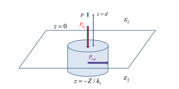
Figure 1: Color online. A vertical dipole is located a distance $d$ above an interface separating linear media characterized by permittivities $\epsilon_{1}$ and $\epsilon_{2}.$ The dipole is driven to emit optical radiation having frequency $\omega=k_{1}c$. The cylindrical volume shown is used to calculate power flow in the normal and radial directions.

In the case of a metal, we assume that

$$\epsilon_{r}<-1\text{ \ \ and \ \ \ \ \ \ }\epsilon_{i}\ll 1.\text{\ }$$ (3)

Moreover, we use the Drude model to characterize the metal. In the Drude model, the complex permittivity $\epsilon_{2}$ is given by

$$\epsilon_{2}=1-\frac{\omega_{p}^{2}}{\omega\left(\omega+i\gamma_{d}\right)}\simeq 1-\frac{\omega_{p}^{2}}{\omega^{2}}+i\frac{\omega_{p}^{2}\gamma_{d}}{\omega^{3}},$$ (4)

where $\omega_{p}$ is the plasma frequency and it has been assumed that $\gamma_{d}\ll\omega$. It then follows that

$$\epsilon_{r}=\frac{1}{\epsilon_{1}}\left(1-\frac{\omega_{p}^{2}}{\omega^{2}}\right)\text{ \ \ and \ \ \ \ \ \ }\epsilon_{i}=\frac{1}{\epsilon_{1}}\frac{\omega_{p}^{2}\gamma_{d}}{\omega^{3}}.\text{\ }$$ (5)

A permittivity $\epsilon_{r}<-1$ corresponds to an input frequency that is below the surface plasmon resonance frequency, $\omega_{sp}=\omega_{p}/\sqrt{1+\epsilon_{1}}$ sp . At frequencies below $\omega_{sp}$, it is possible for the near field of the dipole to excite surface plasmon modes in the metal. For $-1<\epsilon_{r}<0$, there is no surface plasmon resonance, but it is still possible to excite evanescent lateral waves in medium 2.

It is convenient to define an effective conductivity $\sigma$ by setting

$$\epsilon_{2}=\epsilon_{2r}+\frac{4\pi i\sigma}{\omega}$$ (6)

or

$$\epsilon=\epsilon_{2}/\epsilon_{1}=\epsilon_{r}+\frac{4\pi i\sigma}{\omega\epsilon_{1}}$$ (7)

which implies that

$$\sigma=\frac{\epsilon_{i}\omega\epsilon_{1}}{4\pi}.$$ (8)

The conductivity leads to ”Joule heating” in the metal, but it should be noted that this conductivity could also account for radiative losses associated with the scattering of radiation by the metal.

To model a lossless dielectric, we take

$$\text{\ }\epsilon_{r}>0\text{ \ \ \ \ and \ \ \ \ \ \ }\epsilon_{i}=0\text{\ }.$$ (9)

In all calculations, we keep terms in the power flow that are at most first order in $\epsilon_{i}$ and often zeroth order in $\epsilon_{i}$.

All electromagnetic fields, as well as the Hertz vector, have the same time dependence $(e^{-i\omega t})$, which is suppressed throughout this paper. In cylindrical coordinates, the Hertz vectors in media 1 and 2 are given by som ; sil , silcorr

$$\mathbf{\Pi}_{1}(\tilde{\rho},\tilde{z}) =\mathbf{\hat{z}}k_{1}p\int_{0}^{\infty}\frac{u}{\ell_{1}}J_{0}(u\tilde{\rho})\left[e^{\pm\ell_{1}\left(\tilde{z}-\tilde{d}\right)}+f_{1}e^{-\ell_{1}\left(\tilde{z}+\tilde{d}\right)}\right]=\Pi_{1}(\tilde{\rho},\tilde{z})\mathbf{\hat{z}}$$ (10a)

$$\mathbf{\Pi}_{2}(\tilde{\rho},\tilde{z}) =\mathbf{\hat{z}}k_{1}p\int_{0}^{\infty}\frac{u}{\ell_{1}}J_{0}(u\tilde{\rho})e^{-\ell_{1}\tilde{d}}f_{2}e^{\ell_{2}\tilde{z}}=\Pi_{2}(\tilde{\rho},\tilde{z})\mathbf{\hat{z}}$$ (10b)

where $$J_{0}$$ is a Bessel function,

$$k_{1} =\sqrt{\epsilon_{1}\mu_{1}}\omega/c$$ (11a)

$$\tilde{\rho} =k_{1}\rho$$ (11b)

$$\tilde{z} =k_{1}z$$ (11c)

$$\tilde{d} =k_{1}d$$ (11d)

$$\ell_{1} =-i\sqrt{1-u^{2}}$$ (11e)

$$\ell_{2} =-i\sqrt{\epsilon\mu-u^{2}}$$ (11f)

$$f_{1} =\frac{\epsilon\ell_{1}-\ell_{2}}{\epsilon\ell_{1}+\ell_{2}}$$ (11g)

$$f_{2} =\frac{2\epsilon\ell_{1}}{\epsilon\ell_{1}+\ell_{2}}.$$ (11h)

The $$+ z<d - z>d \ell_{2} \mu \mu \ell_{2}=\pm i\sqrt{\epsilon\mu-u^{2}} \operatorname{Re}\ell_{2}>0$$ sign is taken for and the sign for . The value of is written for real and positive; for arbitrary values of , with the sign chosen such that . The fields are given by

$$\mathbf{E}_{1} =\frac{1}{\epsilon_{1}}\nabla\times\nabla\times\mathbf{\Pi}_{1}$$ (12a)

$$\mathbf{H}_{1} =\mathbf{B}_{1}/\mu_{1}=-i\frac{\omega}{c}\nabla\times\mathbf{\Pi}_{1}$$ (12b)

$$\mathbf{E}_{2} =\frac{1}{\epsilon_{1}\epsilon}\nabla\times\nabla\times\mathbf{\Pi}_{2}$$ (12c)

$$\mathbf{H}_{2} =\mathbf{B}_{2}/\mu_{2}=-i\frac{\omega}{c}\nabla\times\mathbf{\Pi}_{2}.$$ (12d)

For the most part, we concentrate on the fields in medium 2 only. If one is interested in the fields in medium 1, it turns out that some computational problems can be avoided by rewriting Eq. (10a) as

$$\Pi_{1}(\tilde{\rho},\tilde{z}) =k_{1}p\int_{0}^{\infty}\frac{u}{\ell_{1}}J_{0}(u\tilde{\rho})f_{1}e^{-\ell_{1}\left(\tilde{z}+\tilde{d}\right)}$$

$$+\frac{k_{1}p\exp\left[i\sqrt{\tilde{\rho}^{2}+\left(\tilde{z}-\tilde{d}\right)^{2}}\right]}{\sqrt{\tilde{\rho}^{2}+\left(\tilde{z}-\tilde{d}\right)^{2}}}.$$ (13)

Note that this expression is valid for any $z>0.$ Although $\ell_{1}$ is a function of $u,$ $\ell_{2}$ is a function of $\epsilon$, $\mu$ and $u$, and both $f_{1}$ and $f_{2}$ are functions of $\epsilon$, $\mu$, and $u$, the explicit dependence of these functions on $\epsilon$, $\mu$ and $u$ is suppressed except when there is some cause for confusion. The Hertz vectors given by Eq. (10) satisfy the boundary conditions silcorr

$$\Pi_{1}(z=0) =\Pi_{2}(z=0);$$ (14a)

$$\epsilon\frac{\partial\Pi_{1}(z=0)}{\partial z} =\frac{\partial\Pi_{2}(z=0)}{\partial z},$$ (14b)

which guarantee that $$\mathbf{H}_{\phi} \mathbf{E}_{\rho} \mathbf{D}_{z}$$, , and are continuous at the interface.

The fields in medium 2 are

$$\mathbf{E}_{2} =\frac{k_{1}^{2}}{\epsilon_{1}\epsilon}\left[\frac{\partial^{2}\Pi_{2}}{\partial\tilde{\rho}\partial\tilde{z}}\mathbf{\hat{\rho}}-\left(\frac{\partial^{2}\Pi_{2}}{\partial\tilde{\rho}^{2}}+\frac{1}{\tilde{\rho}}\frac{\partial\Pi_{2}}{\partial\tilde{\rho}}\right)\mathbf{\hat{z}}\right]$$ (15a)

$$\mathbf{H}_{2} =\mathbf{B}_{2}/\mu_{2}=i\frac{\omega}{c}k_{1}\frac{\partial\Pi_{2}}{\partial\tilde{\rho}}\mathbf{\hat{\phi},}$$ (15b)

the time-averaged Poynting vector in medium 2, $$\mathbf{S}_{2}$$, is

$$\mathbf{S}_{2} =\frac{c}{8\pi}\operatorname{Re}\left(\mathbf{E}_{2}\times\mathbf{H}_{2}^{\ast}\right)$$

$$=\frac{k_{1}^{3}\omega}{8\pi\epsilon_{1}}\operatorname{Re}\left\{\left(\frac{-i}{\epsilon}\right)\left[\frac{\partial^{2}\Pi_{2}}{\partial\tilde{\rho}\partial\tilde{z}}\frac{\partial\Pi_{2}^{\ast}}{\partial\tilde{\rho}}\mathbf{\hat{z}}+\left(\frac{\partial^{2}\Pi_{2}}{\partial\tilde{\rho}^{2}}+\frac{1}{\tilde{\rho}}\frac{\partial\Pi_{2}}{\partial\tilde{\rho}}\right)\frac{\partial\Pi_{2}^{\ast}}{\partial\tilde{\rho}}\mathbf{\hat{\rho}}\right]\right\},$$ (16)

and the time-averaged ”Joule heating” is hcont

$$J=\frac{1}{2}\sigma\int_{\text{volume}}\mathbf{E}_{2}\mathbf{\cdot E}_{2}^{\ast}d\tau=\frac{\epsilon_{i}\omega\epsilon_{1}}{8\pi}\int_{\text{volume}}\mathbf{E}_{2}\mathbf{\cdot E}_{2}^{\ast}d\tau.$$ (17)

The fields and time-averaged Poynting vector in medium 1 are given by Eqs. (15) and (16), respectively, with $\Pi_{2}$ replaced by $\Pi_{1}$ and $\epsilon$ replaced by unity.

From elementary properties of Bessel functions, it follows that

$$\frac{\partial^{2}\Pi_{2}}{\partial\tilde{\rho}\partial\tilde{z}} =-k_{1}p\int_{0}^{\infty}\frac{\ell_{2}u^{2}}{\ell_{1}}J_{1}(u\tilde{\rho})e^{-\ell_{1}\tilde{d}}f_{2}e^{\ell_{2}\tilde{z}}du\equiv-k_{1}pI_{1},$$ (18a)

$$\left(\frac{\partial^{2}\Pi_{2}}{\partial\tilde{\rho}^{2}}+\frac{1}{\tilde{\rho}}\frac{\partial\Pi_{2}}{\partial\tilde{\rho}}\right) =-k_{1}p\int_{0}^{\infty}\frac{u^{3}}{\ell_{1}}J_{0}(u\tilde{\rho})e^{-\ell_{1}\tilde{d}}f_{2}e^{\ell_{2}\tilde{z}}du\equiv-k_{1}pI_{2},$$ (18b)

$$\frac{\partial\Pi_{2}^{\ast}}{\partial\tilde{\rho}} =-k_{1}p\int_{0}^{\infty}\frac{u^{2}}{\ell_{1}^{\ast}}J_{1}(u\tilde{\rho})e^{-\ell_{1}^{\ast}\tilde{d}}f_{2}^{\ast}e^{\ell_{2}^{\ast}\tilde{z}}du\equiv-k_{1}pI_{3}.$$ (18c)

As a consequence,

$$\mathbf{E}_{2} =-\frac{k_{1}^{3}p}{\epsilon_{1}\epsilon}\left[I_{1}\mathbf{\hat{\rho}}-I_{2}\mathbf{\hat{z}}\right]$$ (19a)

$$\mathbf{H}_{2} =\mathbf{B}_{2}/\mu_{2}=-i\frac{\omega}{c}k_{1}^{2}pI_{3}^{\ast}\mathbf{\hat{\phi},}$$ (19b)

$$\mathbf{S}_{2}=-\frac{k_{1}^{5}\omega p^{2}}{8\pi\epsilon_{1}}\operatorname{Re}\left\{\left(\frac{i}{\epsilon}\right)\left[I_{1}I_{3}\mathbf{\hat{z}}+I_{2}I_{3}\mathbf{\hat{\rho}}\right]\right\},$$ (20)

and

$$J=\frac{\epsilon_{i}\omega k_{1}^{6}p^{2}}{8\pi\epsilon_{1}\left|\epsilon\right|^{2}}\int_{\text{volume}}\left(\left|I_{1}\right|^{2}+\left|I_{2}\right|^{2}\right)d\tau.$$ (21)

Using the above equations, one can calculate the power entering medium 2, the Joule heating in the medium, and the radial Poynting vector. When Eq. (6) is satisfied and medium 2 is linear and isotropic (as has been assumed), it follows that Poynting’s theorem holds for any closed surface in medium 2; that is hcont ,

$${\displaystyle\oint}\mathbf{S\cdot}d\mathbf{a=}\int_{vol}Jd\tau$$ (22)

For the fields given by Eq. (15), it is possible to prove this explicitly for a cylindrical surface in medium 2 whose axis is along the $z-$axis. Poynting’s theorem can be used as a check of the numerical accuracy of the solutions.

The general structure of Eqs. (10) allows one to draw some conclusions concerning the nature of the fields in each medium. The parameter $u$ in these equations is equal to $\left(\mathbf{k}_{1}\right)_{\rho}/k_{1}$ and would be equal to the sine of the angle of incidence for incident plane waves. In the case of dipole emission, $u$ can take on values greater than unity, resulting in evanescent ”reflected” waves in medium 1. The influence of these evanescent waves on the transmitted radiation is discussed below. However, we note here that the functions $f_{1}$ and $f_{2}$ exhibit surface plasmon resonance structure as a function of $u$ only for $\epsilon_{r}<-1$ and $\mu>0.$

There is an additional feature having particular relevance for the ensuing development. The boundary conditions on the fields at the surface require that

$$S_{1z}(z =0)=S_{2z}(z=0)$$ (23a)

$$\frac{S_{1\rho}(z=0)}{S_{2\rho}(z=0)} =\frac{\operatorname{Re}\left[\epsilon\mathbf{E}_{2z}(z=0)\mathbf{H}_{2\phi}(z=0)\right]}{\operatorname{Re}\left[\mathbf{E}_{2z}(z=0)\mathbf{H}_{2\phi}(z=0)\right]}$$ (23b)

The energy flow normal to the surface is continuous , but the radial component of the Poynting vector undergoes a jump at the interface. Moreover, if $$\epsilon_{r}<0 \epsilon_{i}\ll 1$$ and , the radial Poynting vector in medium 2 is in a direction opposite to that in medium 1.

III Metal

In this section we consider a metal having $\mu=1$,

$$\epsilon_{r} <-1;$$ (24a)

$$\epsilon_{i} \ll 1,$$ (24b)

and keep terms in the power flow that are zeroth or first order in $$\epsilon_{i} \mu \epsilon \tilde{\rho} \epsilon_{r}\sim-\infty \epsilon_{i}=0.$$. Although the asymptotic results that are derived in this section are valid only in these limits, the general expressions from which these asymptotic results are derived are valid for arbitrary and . When inequalities (24) are satisfied, there is coupling of the dipole field into surface plasmon waves sp . Such fields are evanescent since their magnitudes decrease exponentially as a function of the distance from the surface. However, these lateral fields propagate parallel to the surface with amplitudes that fall off very slowly with increasing . The limit of a perfect metal is achieved by setting and In that limit, the problem could be solved by the method of images.

III.1 Power into medium 2

The total power entering medium 2 is given by

$$P_{in} =-\frac{2\pi}{k_{1}^{2}}\int_{0}^{\infty}\tilde{\rho}d\tilde{\rho}\left.S_{2z}\right|_{\tilde{z}=0}=\frac{2\pi}{k_{1}^{2}}\frac{k_{1}^{5}p^{2}\omega}{8\pi\epsilon_{1}}\int_{0}^{\infty}\tilde{\rho}d\tilde{\rho}\left.\operatorname{Re}\left\{\left(\frac{i}{\epsilon}\right)I_{1}I_{3}\right\}\right|_{\tilde{z}=0}$$

$$=\frac{k_{1}^{3}p^{2}\omega}{4\epsilon_{1}}\int_{0}^{\infty}\tilde{\rho}d\tilde{\rho}\operatorname{Re}\left\{\begin{array}[c]{c}\left(\frac{i}{\epsilon}\right)\int_{0}^{\infty}\frac{\ell_{2}u^{2}}{\ell_{1}}J_{1}(u\tilde{\rho})e^{-\ell_{1}\tilde{d}}f_{2}du\\ \times\int_{0}^{\infty}\frac{u^{\prime 2}}{\ell_{1}^{\ast}}J_{1}(u^{\prime}\tilde{\rho})e^{-\ell_{1}^{\ast}\tilde{d}}f_{2}^{\ast}du^{\prime}\end{array}\right\}.$$ (27)

Using

$$\int_{0}^{\infty}\tilde{\rho}d\tilde{\rho}J_{\nu}(u\tilde{\rho})J_{\nu}(u^{\prime}\tilde{\rho})=\frac{\delta\left(u-u^{\prime}\right)}{u},$$ (28)

we find

$$P_{in} =\frac{k_{1}^{3}p^{2}\omega}{4\epsilon_{1}}\operatorname{Re}\left\{\left(\frac{i}{\epsilon}\right)\int_{0}^{\infty}\frac{\ell_{2}u^{3}}{\ell_{1}\ell_{1}^{\ast}}e^{-\ell_{1}\tilde{d}}f_{2}f_{2}^{\ast}e^{-\ell_{1}^{\ast}\tilde{d}}du\right\}$$

$$=\frac{k_{1}^{3}p^{2}\omega\left|\epsilon\right|^{2}}{\epsilon_{1}}\operatorname{Re}\left\{\left(\frac{i}{\epsilon}\right)\int_{0}^{\infty}\frac{\ell_{2}u^{3}}{\left|\epsilon\ell_{1}+\ell_{2}\right|^{2}}e^{-\left(\ell_{1}+\ell_{1}^{\ast}\right)\tilde{d}}du\right\}.$$ (29)

This integral can be evaluated numerically for arbitrary $\mu$ and $\epsilon$. However, for $\mu=1,$ $\epsilon_{r}<-1$ and $\epsilon_{i}\ll 1$ (the limiting values considered in this section), it is shown in the appendix that, to zeroth order in $\epsilon_{i}$,

$$P_{in}=\frac{k_{1}^{3}p^{2}\omega\pi\left|\epsilon_{r}\right|^{3}e^{-2\sqrt{\frac{1}{\left|\epsilon_{r}\right|-1}}\tilde{d}}}{\epsilon_{1}\left(\left|\epsilon_{r}\right|-1\right)^{5/2}\left(\left|\epsilon_{r}\right|+1\right)},$$ (30)

a result in agreement with that obtained by previous authors sil ; ford . Owing to surface plasmons, there can now be substantial energy flow into the medium, especially for frequencies close to the surface plasmon resonance frequency $\omega_{sp}=\omega_{p}/\sqrt{1+\epsilon_{1}}$ for which $\epsilon_{r}=-1$.

III.2 Joule Heating

From Eq. (21) we can calculate the total rate of Joule heating as

$$J=\frac{\epsilon_{i}\omega k_{1}^{3}p^{2}}{4\epsilon_{1}\left|\epsilon\right|^{2}}\int_{0}^{\infty}\tilde{\rho}d\tilde{\rho}\int_{-\infty}^{0}d\tilde{z}\left\{\begin{array}[c]{c}\left|\int_{0}^{\infty}\frac{\ell_{2}u^{2}}{\ell_{1}}J_{1}(u\tilde{\rho})e^{-\ell_{1}\tilde{d}}f_{2}e^{\ell_{2}\tilde{z}}du\right|^{2}\\ +\left|\int_{0}^{\infty}\frac{u^{3}}{\ell_{1}}J_{0}(u\tilde{\rho})e^{-\ell_{1}\tilde{d}}f_{2}e^{\ell_{2}\tilde{z}}du\right|^{2}\end{array}\right\}.$$ (31)

Using Eq. (28), we find

$$J=\frac{\epsilon_{i}\omega k_{1}^{3}p^{2}}{4\epsilon_{1}\left|\epsilon\right|^{2}}\int_{0}^{\infty}du\frac{u^{3}}{\left|\ell_{1}\right|^{2}}e^{-\left(\ell_{1}+\ell_{1}^{\ast}\right)\tilde{d}}\left|f_{2}\right|^{2}\frac{\left(\left|\ell_{2}\right|^{2}+u^{2}\right)}{\ell_{2}+\ell_{2}^{\ast}}.$$ (32)

To zeroth order in $\epsilon_{i}$ and with $\mu=1$ and $\epsilon_{r}<-1$, Eq. (32) reduces to (see appendix)

$$J=\frac{k_{1}^{3}p^{2}\omega\pi\left|\epsilon_{r}\right|^{3}e^{-2\sqrt{\frac{1}{\left|\epsilon_{r}\right|-1}}\tilde{d}}}{\epsilon_{1}\left(\left|\epsilon_{r}\right|-1\right)^{5/2}\left(\left|\epsilon_{r}\right|+1\right)},$$ (33)

which is identical to Eq. (30). All the input intensity is converted to Joule heating.

III.3 Radial Power

We now calculate the outgoing radial field power $P_{rad}$ passing through the cylindrical surface of an infinite cylinder in the lower half plane (that is, a cylinder extending from $z=0$ to $z=-\infty$) having radius $r=\tilde{r}/k_{1}$ (see Fig. 1). In other words, we calculate

$$P_{rad} =\frac{2\pi\tilde{r}}{k_{1}^{2}}\int_{-\infty}^{0}S_{2\rho}d\tilde{z}=\frac{2\pi\tilde{r}}{k_{1}^{2}}\frac{k_{1}^{5}p^{2}\omega}{8\pi\epsilon_{1}}\int_{-\infty}^{0}d\tilde{z}\operatorname{Re}\left[\left(\frac{-i}{\epsilon}\right)I_{2}I_{3}\right]$$

$$=\frac{k_{1}^{3}p^{2}\omega\tilde{r}}{4\epsilon_{1}}\operatorname{Re}\left\{\begin{array}[c]{c}\left(-\frac{i}{\epsilon}\right)\int_{0}^{\infty}du\int_{0}^{\infty}du^{\prime}\frac{u^{3}}{\ell_{1}(u)}J_{0}(u\tilde{r})e^{-\ell_{1}(u)\tilde{d}}f_{2}(u)\\ \times\frac{u^{\prime 2}}{\ell_{1}^{\ast}(u^{\prime})}J_{1}(u^{\prime}\tilde{r})e^{-\ell_{1}^{\ast}(u^{\prime})\tilde{d}}f_{2}^{\ast}(u^{\prime})\frac{1}{\ell_{2}(u)+\ell_{2}^{\ast}(u^{\prime})}\end{array}\right\}.$$ (36)

It is shown in the appendix that for $\tilde{r}\gg 1$, $\mu=1,$ $\epsilon_{r}<-1,$ and $\epsilon_{i}\ll 1$, $P_{rad}$ takes on the asymptotic limit

$$P_{rad}(asy)\sim-\frac{k_{1}^{3}p^{2}\omega\pi e^{-2\sqrt{\frac{1}{\left|\epsilon_{r}\right|-1}}\tilde{d}}e^{-\epsilon_{i}^{\prime}\tilde{r}}}{\epsilon_{1}}\frac{\left|\epsilon_{r}\right|^{3}}{\left(\left|\epsilon_{r}\right|-1\right)^{7/2}\left(\left|\epsilon_{r}\right|+1\right)^{2}}.$$ (37)

As $\tilde{r}\sim\infty$, $P_{rad}\sim 0$, which is consistent with the fact that $P_{in}=J$. Equation (37) is remarkable in two ways. First, we see that $P_{rad}(asy)$ is negative, implying energy flow in the inward radial direction in the metal. Moreover, for $\epsilon_{i}^{\prime}\tilde{r}<1,$ the magnitude of $P_{rad}$ can be significantly larger than both $P_{in}$ and $J$. Thus it would appear that energy is not conserved. However appearances can be deceiving.

III.4 Power In and Joule Heating for $\tilde{\rho}<\tilde{r}$

To resolve this apparent paradox, we must calculate the Joule heating and input power for the cylinder considered in the discussion of the radial power flow (see Fig. 1). That is, we must show that

$$P_{in_{r}}=P_{rad}+J_{r},$$ (38)

where $J_{r}$ is rate of Joule heating in the volume and $P_{in_{r}}$ is the net power flow into the medium through the end caps of the volume.

III.4.1 Joule heating

The rate of Joule heating for the volume defined by $\tilde{\rho}<\tilde{r}$ and $-\infty<\tilde{z}\leq 0$ (this is the volume enclosed by the surface used to calculate $P_{rad}$) is given by

$$J_{r}=\frac{\epsilon_{i}\omega k_{1}^{3}p^{2}}{4\epsilon_{1}\left|\epsilon\right|^{2}}\int_{0}^{\tilde{r}}\tilde{\rho}d\tilde{\rho}\int_{-\infty}^{0}d\tilde{z}\left\{\begin{array}[c]{c}\left|\int_{0}^{\infty}\frac{\ell_{2}u^{2}}{\ell_{1}}J_{1}(u\tilde{\rho})e^{-\ell_{1}\tilde{d}}f_{2}e^{\ell_{2}\tilde{z}}du\right|^{2}\\ +\left|\int_{0}^{\infty}\frac{u^{3}}{\ell_{1}}J_{0}(u\tilde{\rho})e^{-\ell_{1}\tilde{d}}f_{2}e^{\ell_{2}\tilde{z}}du\right|^{2}\end{array}\right\}.$$ (39)

The integrals over $\tilde{\rho}$ can be done analytically since

$$a(u,u^{\prime},\tilde{r}) =\int_{0}^{\tilde{r}}\tilde{\rho}d\tilde{\rho}J_{1}(u\tilde{\rho})J_{1}(u^{\prime}\tilde{\rho})=\tilde{r}\frac{u^{\prime}J_{0}(u^{\prime}\tilde{r})J_{1}(u\tilde{r})-uJ_{0}(u\tilde{r})J_{1}(u^{\prime}\tilde{r})}{u^{2}-u^{\prime 2}}$$ (40a)

$$b(u,u^{\prime},\tilde{r}) =\int_{0}^{\tilde{r}}\tilde{\rho}d\tilde{\rho}J_{0}(u\tilde{\rho})J_{0}(u^{\prime}\tilde{\rho})=\tilde{r}\frac{uJ_{0}(u^{\prime}\tilde{r})J_{1}(u\tilde{r})-u^{\prime}J_{0}(u\tilde{r})J_{1}(u^{\prime}\tilde{r})}{u^{2}-u^{\prime 2}}.$$ (40b)

Therefore,

$$J_{r}=\frac{\epsilon_{i}\omega k_{1}^{3}p^{2}}{\epsilon_{1}}\left\{\begin{array}[c]{c}\int_{0}^{\infty}du\int_{0}^{\infty}du^{\prime}\frac{\ell_{2}(u)\left[\ell_{2}(u^{\prime})\right]^{\ast}u^{2}u^{\prime 2}e^{-\ell_{1}(u)\tilde{d}}e^{-\ell_{1}^{\ast}(u^{\prime})\tilde{d}}a(u,u^{\prime},\tilde{r})}{\left[\epsilon\ell_{1}(u)+\ell_{2}(u)\right]\left[\epsilon\ell_{1}(u^{\prime})+\ell_{2}(u^{\prime})\right]^{\ast}\left[\ell_{2}(u)+\ell_{2}^{\ast}(u^{\prime})\right]}\\ +\int_{0}^{\infty}du\int_{0}^{\infty}du^{\prime}\frac{u^{3}u^{\prime 3}e^{-\ell_{1}(u)\tilde{d}}e^{-\ell_{1}^{\ast}(u^{\prime})\tilde{d}}b(u,u^{\prime},\tilde{r})}{\left[\epsilon\ell_{1}(u)+\ell_{2}(u)\right]\left[\epsilon\ell_{1}(u^{\prime})+\ell_{2}(u^{\prime})\right]^{\ast}\left[\ell_{2}(u)+\ell_{2}^{\ast}(u^{\prime})\right]}\end{array}\right\}.$$ (41)

These integrals can be evaluated numerically. When $\mu=1,$ $\epsilon_{r}<-1$ and $\epsilon_{i}\ll 1$, the major contributions come from $u\approx u^{\prime}\approx u_{0},$ where

$$u_{0}=\sqrt{\epsilon_{r}/\left(1+\epsilon_{r}\right)}.$$ (42)

As expected, $J_{r}<J$. No surprise. In the limit of large $\tilde{r}$ (see appendix),

$$J_{r}(asy)\sim\frac{\pi\omega k_{1}^{3}p^{2}}{\epsilon_{1}}\frac{\left|\epsilon_{r}\right|^{3}e^{-2\sqrt{\frac{1}{\left|\epsilon_{r}\right|-1}}\tilde{d}}}{\left(\left|\epsilon_{r}\right|-1\right)^{5/2}\left(\left|\epsilon_{r}\right|+1\right)}\left(1-e^{-\epsilon_{i}^{\prime}\tilde{r}}\right),$$ (43)

where

$$\epsilon_{i}^{\prime}=\epsilon_{i}/[\left|\epsilon_{r}\right|^{1/2}\left(\left|\epsilon_{r}\right|-1\right)^{3/2}].$$ (44)

As must be the case, $J_{r}<J$.

III.4.2 Power in

The power flowing into the top cap ($z=0)$ of the cylindrical surface having radius $r=\tilde{r}/k_{1}$ is given by

$$P_{in_{r}} =-\frac{2\pi}{k_{1}^{2}}\int_{0}^{\tilde{r}}\tilde{\rho}d\tilde{\rho}\left.S_{2z}\right|_{\tilde{z}=0}$$

$$=\frac{k_{1}^{3}p^{2}\omega}{\epsilon_{1}}\operatorname{Re}\left\{i\epsilon^{\ast}\int_{0}^{\infty}du\int_{0}^{\infty}du^{\prime}\frac{\ell_{2}(u)u^{2}u^{\prime 2}e^{-\ell_{1}(u)\tilde{d}}e^{-\ell_{1}^{\ast}(u^{\prime})\tilde{d}}a(u,u^{\prime},\tilde{r})}{\left[\epsilon\ell_{1}(u)+\ell_{2}(u)\right]\left[\epsilon\ell_{1}(u^{\prime})+\ell_{2}(u^{\prime})\right]^{\ast}}\right\}.$$ (45)

Since the fields are evanescent, no energy flows out of the bottom cap at $z=-\infty$. The integrals in Eq. (45) can be done numerically, with the major contributions coming from $u\approx u^{\prime}\approx u_{0}$. The result turns out to be somewhat surprising since, for $\epsilon_{i}^{\prime}\tilde{r}\lesssim 1$ the integral is negative! As we shall see, the fact that $P_{in_{r}}<0$ for $\epsilon_{i}^{\prime}\tilde{r}\lesssim 1$ can be attributed to a relatively large energy flow out of the surface for $\tilde{r}\lesssim 1$. In some sense, the power flowing radially inwards in the metal exits the surface at small radii. In this manner energy conservation is restored, as expressed by Eq. (38).

Numerical evaluation of the integrals in Eq. (45) can become somewhat unreliable for very large $\tilde{r}$. For $\tilde{r}>10,$ one can use

$$P_{in_{r}}(asy) =P_{rad}(asy)+J_{r}(asy)$$

$$=\frac{\pi\omega k_{1}^{3}p^{2}}{\epsilon_{1}}\frac{\left|\epsilon_{r}\right|^{3}e^{-2\sqrt{\frac{1}{\left|\epsilon_{r}\right|-1}}\tilde{d}}}{\left(\left|\epsilon_{r}\right|-1\right)^{5/2}\left(\left|\epsilon_{r}\right|+1\right)}\left[\left(1-e^{-\epsilon_{i}^{\prime}r}\right)-\frac{e^{-\epsilon_{i}^{\prime}r}}{\left(\left|\epsilon_{r}\right|^{2}-1\right)}\right]$$ (46)

with minimal error.

To see the dependence of the energy flow direction on $\tilde{r}$, we can calculate the power flowing inwards through a circular ring having radius $\tilde{r}$ and thickness $d\tilde{r}.$ The differential power flowing into this ring is given by

$$\frac{dP_{in_{r}}}{d\tilde{r}}=-\frac{2\pi\tilde{r}}{k_{1}^{2}}\left.S_{2z}\right|_{\tilde{z}=0}=\frac{k_{1}^{3}p^{2}\omega\tilde{r}}{\epsilon_{1}}\operatorname{Re}\left\{\begin{array}[c]{c}\left(i\epsilon^{\ast}\right)\int_{0}^{\infty}\frac{\ell_{2}u^{2}J_{1}(u\tilde{\rho})e^{-\ell_{1}\tilde{d}}du}{\epsilon\ell_{1}+\ell_{2}}\\ \times\int_{0}^{\infty}\frac{u^{\prime 2}J_{1}(u^{\prime}\tilde{\rho})e^{-\ell_{1}^{\ast}\tilde{d}}du^{\prime}}{\left[\epsilon\ell_{1}+\ell_{2}\right]^{\ast}}\end{array}\right\},$$ (47)

which can be evaluated numerically. Since the result is the product of two integrals rather than a double integral, the numerical evaluation does not present any problems. For $\tilde{r}>10,$ the asymptotic result

$$\frac{dP_{inr}(asy)}{d\tilde{r}} =\frac{dP_{rad}(asy)}{d\tilde{r}}+\frac{dJ_{r}(asy)}{d\tilde{r}}$$

$$=\frac{\pi\epsilon_{i}\omega k_{1}^{3}p^{2}}{\epsilon_{1}}\frac{\left|\epsilon_{r}\right|^{9/2}e^{-2\sqrt{\frac{1}{\left|\epsilon_{r}\right|-1}}\tilde{d}}e^{-\epsilon_{i}\tilde{r}/\left(\sqrt{-\epsilon_{r}}\left(\left|\epsilon_{r}\right|-1\right)^{3/2}\right)}}{\left(\left|\epsilon_{r}\right|-1\right)^{5}\left(\left|\epsilon_{r}\right|+1\right)^{2}}$$ (48)

agrees with the numerical result to within 1%. The expression for $dP_{inr}(asy)/d\tilde{r}$, valid for large values of $\tilde{r}$, is positive and decreases monotonically with increasing $\tilde{r}.$

III.5 Numerical results

We now present some graphs for $P_{in_{r}},$ $P_{rad}$, and $dP_{in_{r}}/d\tilde{r}$ . In all cases we use exact integral expressions (correct to any order in $\epsilon_{i}$) and take $\mu=1$,

$$\epsilon =\epsilon_{r}+i\epsilon_{i}=-1.1+0.001i$$ (49)

$$\tilde{d} =0.5$$ (50)

which implies that

$$u_{0}=3.32\text{ \ \ \ \ \ \ }\epsilon_{i}^{\prime}=0.0316.$$ (51)

In the Drude model, the value of $\epsilon_{r}=-1.1$ corresponds to a frequency $\omega=0.69\omega_{p}$ slightly below the surface plasmon resonance frequency $\omega=\omega_{p}/\sqrt{2}$ for $\epsilon_{1}=1$. For the chosen value of $\tilde{d}$ the integrals converge rapidly for large values of $u$ or $u^{\prime}$ since the integrands vary as $e^{-u\tilde{d}}$ or $e^{-u^{\prime}\tilde{d}}$ in this limit. However for large $\tilde{r}$, the integrands oscillate rapidly and a check of energy conservation indicates that there are numerical errors. For $\tilde{r}>40,$ one can use Eq. (46). With the chosen parameters,

$$P_{in}=J=159P_{0},$$ (52)

where

$$P_{0}=\frac{\omega k_{1}^{3}p^{2}}{6\epsilon_{1}}$$ (53)

is the total power radiated by a dipole into the lower half plane in a uniform medium having permittivity $\epsilon_{1}$.

A plot of $P_{in_{r}}/P_{0}$ vs $\tilde{r}$ is given in Fig. 2. Recall that $P_{in_{r}}$ is the net power flowing into the cap of a circular surface having radius $\tilde{r}$ whose axis is the $z-$axis. We see that $P_{in_{r}}$ is negative for $\tilde{r}\lesssim 60$, but eventually approaches the asymptotic value for the total power $P_{in}$ entering the surface given by Eq. (52). There is a large enhancement factor in the transmitted energy [$P_{in_{r}}(\infty)/P_{0}\gg 1$] owing to the fact that the oscillation frequency of the dipole is close to, but below, the surface plasmon resonance frequency. In Fig. 3, $-P_{rad}/P_{0}$ is plotted as a function of $\tilde{r}$ (recall the $-P_{rad}$ is the power flowing radially inwards through the cylindrical surface of an infinite cylinder in the lower half plane having radius $r=\tilde{r}/k_{1}$). As predicted, the radial flow is always inwards.

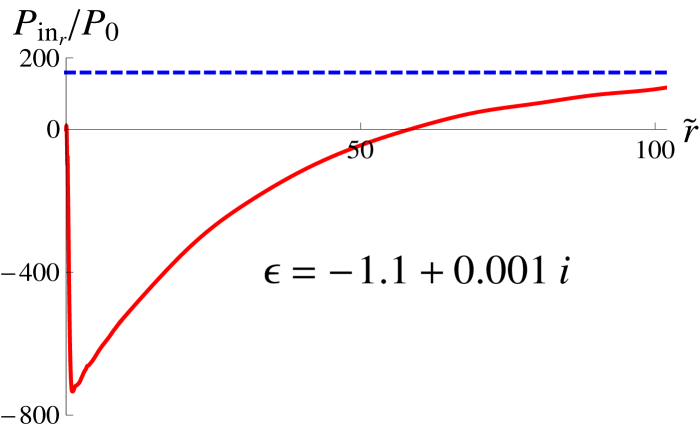
Figure 2: Color online. $P_{in_{r}}/P_{0}$ vs $\tilde{r}$ for $\epsilon=-1.1+0.001i$ (solid curve); The dashed line represents the total power entering the interface, $P_{in_{r}}(\infty)/P_{0}.$ In this and all other figures, $\mu=1$, unless noted otherwise.

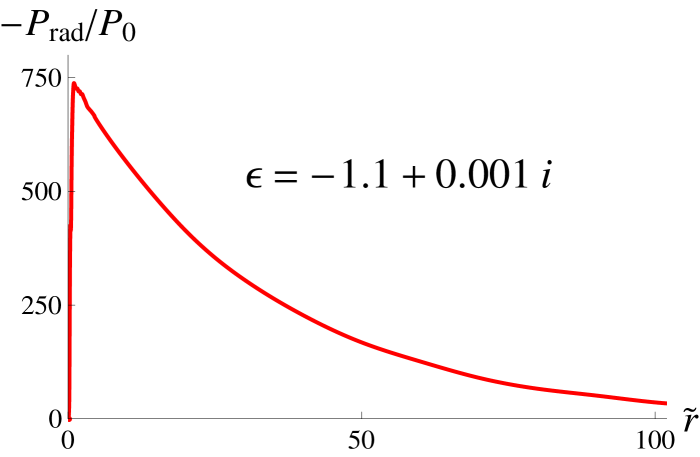
Figure 3: Color online. -$P_{rad}/P_{0}$ vs $\tilde{r}$ for $\epsilon=-1.1+0.001i$ . The power flow is radially inwards in the metal.

In Fig. 4, a graph of $\frac{dP_{in_{r}}}{d\tilde{r}}/P_{0}$ is shown as a function of $\tilde{r}$ (recall that $\frac{dP_{in_{r}}}{d\tilde{r}}d\tilde{r}$ is the power flowing into a circular ring on the surface having radius $\tilde{r}$ and thickness $d\tilde{r}).$ The differential power flowing into this ring starts at zero, grows negatively, reaches a minimum and then turns positive. Oscillations are seen for positive values of $\tilde{r}$ in the blow-up shown in Fig. 5. The asymptotic solution [Eq. (48)] is superimposed on the graph in Fig. 5. It fails to produce the oscillations; instead it seems to track the average value of the oscillations. The physical origin of the oscillations is not clear to us, but similar oscillations occur for the surface charge density. The oscillations are a near field effect that are present when surface plasmon modes are excited by the driving field.

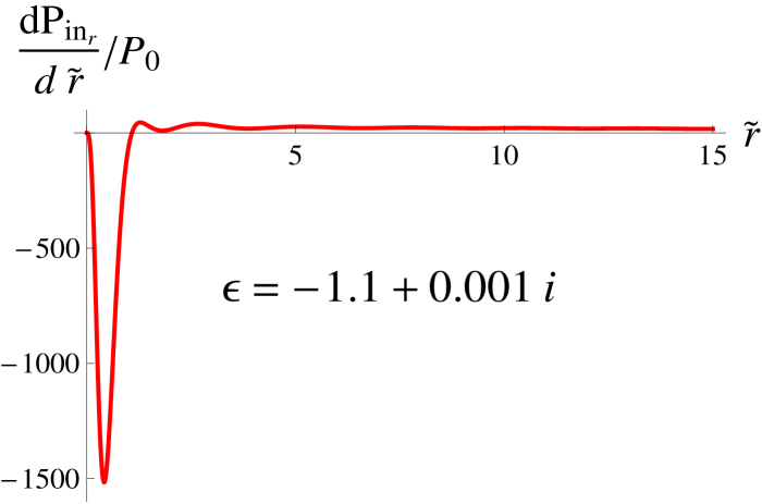
Figure 4: Color online. Differential power flow entering the interface in a ring having radius $\tilde{r}$ and thickness $d\tilde{r}$ for $\epsilon=-1.1+0.001i$. At small $\tilde{r}$ the power flow is out of the metal.

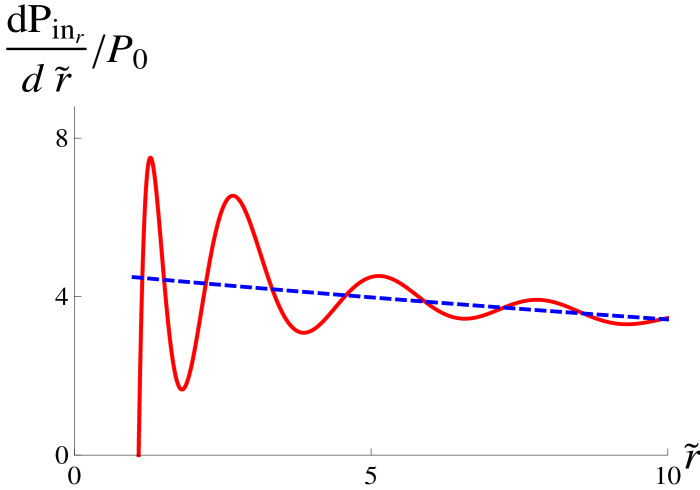
Figure 5: Color online. A blow-up of Fig. 4 showing oscillations. The dashed curve is the asymptotic form given in Eq. (48).

IV Dielectric

We now consider the limit of a lossless dielectric in which $\epsilon$ is real and greater than zero and $\mu=1$. In this limit there is no Joule heating and all the power entering the dielectric either propagates downwards through the dielectric or parallel to the interface in the form of lateral waves. The formalism is the same as in the case for $\epsilon_{r}<-1$, but the values of the integrals differ. We consider two limits, $\epsilon>1$ and $0<\epsilon<1$.

For plane waves incident on an interface with $\epsilon>1$, the maximum angle of refraction is

$$\theta_{2\max}=\sin^{-1}\left(1/\sqrt{\epsilon}\right)\text{.}$$ (54)

On the other hand, for plane waves incident on an interface with $0<\epsilon<1,$ there is total internal reflection for angles of incidence greater than

$$\theta_{1\text{c}}=\sin^{-1}\sqrt{\epsilon}\text{.}$$ (55)

In neither case is it possible to have $S_{z}>0$ at $z=0.$

IV.1 $\epsilon>1$

IV.1.1 Power into and out of medium 2

As before, the total power into medium 2 is given by

$$P_{in}=\frac{k_{1}^{3}p^{2}\omega\epsilon}{\epsilon_{1}}\operatorname{Re}\left\{i\int_{0}^{\infty}\frac{\ell_{2}u^{3}}{\left|\epsilon\ell_{1}+\ell_{2}\right|^{2}}e^{-\left(\ell_{1}+\ell_{1}^{\ast}\right)\tilde{d}}du\right\}.$$ (56)

If we take $\epsilon>1$, the integrand is purely real for $u>\sqrt{\epsilon}$. Thus we can set

$$P_{in}=\frac{k_{1}^{3}p^{2}\omega}{\epsilon_{1}}\operatorname{Re}\left\{i\epsilon\int_{0}^{\sqrt{\epsilon}}\frac{\ell_{2}u^{3}}{\left|\epsilon\ell_{1}+\ell_{2}\right|^{2}}e^{-\left(\ell_{1}+\ell_{1}^{\ast}\right)\tilde{d}}du\right\}\equiv\frac{k_{1}^{3}p^{2}\omega}{\epsilon_{1}}I_{in}$$ (57)

Moreover, for $u<1$, both $\ell_{1}$ and $\ell_{2}$ are purely imaginary, while for $1<u<\sqrt{\epsilon}$, $\ell_{1}$ is purely real and $\ell_{2}$ is purely imaginary. Thus

$$I_{in} =\operatorname{Re}\left\{i\epsilon\int_{0}^{\sqrt{\epsilon}}\frac{\ell_{2}u^{3}}{\left|\epsilon\ell_{1}+\ell_{2}\right|^{2}}e^{-\left(\ell_{1}+\ell_{1}^{\ast}\right)\tilde{d}}du\right\}$$

$$=\epsilon\int_{0}^{1}\frac{u^{3}\sqrt{\epsilon-u^{2}}}{\left(\epsilon\sqrt{1-u^{2}}+\sqrt{\epsilon-u^{2}}\right)^{2}}du$$

$$+\epsilon\int_{1}^{\sqrt{\epsilon}}\frac{u^{3}\sqrt{\epsilon-u^{2}}}{\left(\epsilon-1\right)\left[u^{2}\left(\epsilon+1\right)-\epsilon\right]}e^{-2\sqrt{u^{2}-1}\tilde{d}}du.$$ (58)

The first term is independent of $\tilde{d}$ and represents waves propagating into the medium, while the second term can be thought of as refraction of the near field in medium 1 into propagating waves in medium 2. This is a near field effect and results in an enhancement of the power transmitted to the dielectric lk .

To get the power propagating in the medium at any $\tilde{z}$, we must add a factor $e^{-\left(\ell_{2}+\ell_{2}^{\ast}\right)\tilde{z}}$ into each integrand, but since $\ell_{2}$ is purely imaginary, it follows that

$$I(\tilde{z})=I_{in}\text{; \ \ \ \ }\tilde{z}<0;$$ (59)

the power passing through an infinite $xy-$plane in medium 2 is independent of $\tilde{z}.$ A graph of $P_{in}/P_{0}$ vs $\tilde{d}$ is shown as the solid curve in Fig. 6 for $\epsilon=1.4$. The contribution from the second integral dominates for $\tilde{d}<1$.

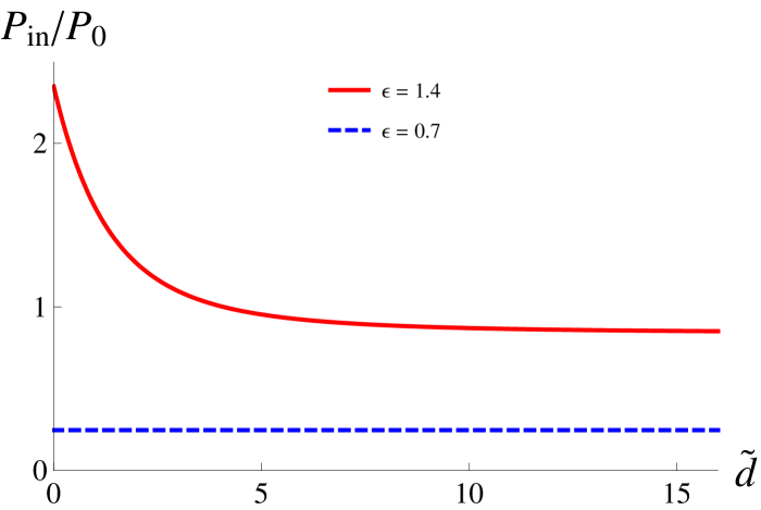
Figure 6: Color online. Total power flow entering the interface $P_{in}/P_{0}$ as a function of $\tilde{d}$ for $\epsilon=1.4$ (solid curve) and $\epsilon=0.7$ (dashed line). The increased power flow for small $\tilde{d}$ and $\epsilon=1.4$ results from near field coupling to propagating modes in the dielectric.

IV.1.2 Radial Power

As before, the power passing radially outwards through a cylinder (that is, through the cylindrical surface of a cylinder whose axis coincides with the $z-$axis and whose end caps are located at $z=0$ and $z=-Z/k_{1}<0$) in the lower half plane having radius $r=\tilde{r}/k_{1}$ is

$$P_{rad}(\tilde{r},Z)=-\frac{k_{1}^{3}p^{2}\omega\tilde{r}}{\epsilon_{1}}\operatorname{Re}\left\{\begin{array}[c]{c}i\epsilon\int_{0}^{\infty}du\int_{0}^{\infty}du^{\prime}u^{3}J_{0}(u\tilde{r})e^{-\ell_{1}(u)\tilde{d}}\frac{1}{\epsilon\ell_{1}(u)+\ell_{2}(u)}\\ \times u^{\prime 2}J_{1}(u^{\prime}\tilde{r})e^{-\ell_{1}^{\ast}(u^{\prime})\tilde{d}}\frac{1}{\left[\epsilon\ell_{1}(u^{\prime})+\ell_{2}(u^{\prime})\right]^{\ast}}\frac{1-\exp\left\{-\left[\ell_{2}(u)+\ell_{2}^{\ast}(u^{\prime})\right]Z\right\}}{\ell_{2}(u)+\ell_{2}^{\ast}(u^{\prime})}\end{array}\right\}.$$ (60)

The integral can be evaluated numerically. In this case the radial flow is outwards and simply represents the radial component of the Poynting vector associated with propagation downwards in medium 2, in contrast to the $\epsilon_{r}<-1$ case where the inwards radial flow corresponds to lateral, evanescent waves.

IV.1.3 Power in medium 2 for $\tilde{\rho}<\tilde{r}$

The power $P_{{}_{r}}$ propagating in medium 2 through a circular surface having radius $r=\tilde{r}/k_{1},$ centered and normal to the $z-$axis at $\tilde{z}=-Z$ is given by

$$P_{{}_{r}}(\tilde{r},\tilde{z}=-Z)=\frac{k_{1}^{3}p^{2}\omega}{\epsilon_{1}}\operatorname{Re}\left\{i\epsilon\int_{0}^{\infty}du\int_{0}^{\infty}du^{\prime}\frac{\ell_{2}(u)u^{2}u^{\prime 2}e^{-\ell_{1}(u)\tilde{d}}e^{-\ell_{1}^{\ast}(u^{\prime})\tilde{d}}a(u,u^{\prime},\tilde{r})e^{-\ell_{2}(u)Z}e^{-\ell_{2}(u^{\prime})Z}}{\left[\epsilon\ell_{1}(u)+\ell_{2}(u)\right]\left[\epsilon\ell_{1}(u^{\prime})+\ell_{2}(u^{\prime})\right]^{\ast}}\right\},$$ (61)

which implies that the net power flowing into the cylinder through the end caps is

$$\delta P_{in_{r}}(\tilde{r},Z) =P_{r}(\tilde{r},0)-P_{r}(\tilde{r},-Z)$$

$$=\frac{k_{1}^{3}p^{2}\omega}{\epsilon_{1}}\operatorname{Re}\left\{\begin{array}[c]{c}i\epsilon\int_{0}^{\infty}du\int_{0}^{\infty}du^{\prime}\frac{\ell_{2}(u)u^{2}u^{\prime 2}e^{-\ell_{1}(u)\tilde{d}}e^{-\ell_{1}^{\ast}(u^{\prime})\tilde{d}}a(u,u^{\prime},\tilde{r})}{\left[\epsilon\ell_{1}(u)+\ell_{2}(u)\right]\left[\epsilon\ell_{1}(u^{\prime})+\ell_{2}(u^{\prime})\right]^{\ast}}\\ \times\left[1-\exp\left\{-\left[\ell_{2}(u)+\ell_{2}^{\ast}(u^{\prime})\right]Z\right\}\right]\end{array}\right\}.$$ (64)

From Poynting’s theorem it follows that

$$\delta P_{in_{r}}(\tilde{r},Z)=P_{rad}(\tilde{r},Z),$$ (65)

since there is no Joule heating.

In Fig. 7, we plot $P_{in_{r}}(\tilde{r})/P_{0}=P_{{}_{r}}(\tilde{r},0)/P_{0}$ as a function of $\tilde{r}$ for $\epsilon=1.4$ and $\tilde{d}=0.5$. Although there is nowhere near the enhancement of the radiation in the $\epsilon\approx-1$ case, there is still some enhancement since $P_{in_{r}}(\infty)/P_{0}>1$, owing to near field refraction. In contrast to the $\epsilon\approx-1$ case, $P_{in_{r}}$ is never negative and increases with increasing $\tilde{r}$.

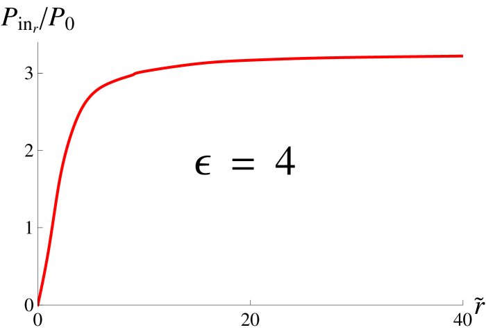
Figure 7: Color online. $P_{in_{r}}/P_{0}$ vs $\tilde{r}$ for $\epsilon=4.$

IV.2 $0<\epsilon<1$

IV.2.1 Power into and out of medium 2

As before, the total power into the medium is given by

$$P_{in}=\frac{k_{1}^{3}p^{2}\omega\epsilon}{\epsilon_{1}}\operatorname{Re}\left\{i\int_{0}^{\sqrt{\epsilon}}\frac{\ell_{2}u^{3}}{\left|\epsilon\ell_{1}+\ell_{2}\right|^{2}}e^{-\left(\ell_{1}+\ell_{1}^{\ast}\right)\tilde{d}}du\right\}.$$ (66)

However since $\epsilon<1$, both $\ell_{1}$ and $\ell_{2}$ are purely imaginary and

$$I_{in} =I(\tilde{z})=\operatorname{Re}\left\{i\int_{0}^{\sqrt{\epsilon}}\frac{\ell_{2}u^{3}}{\left|\epsilon\ell_{1}+\ell_{2}\right|^{2}}e^{-\left(\ell_{1}+\ell_{1}^{\ast}\right)\tilde{d}}du\right\}$$

$$=\int_{0}^{\sqrt{\epsilon}}\frac{u^{3}\sqrt{\epsilon-u^{2}}}{\left(\epsilon\sqrt{1-u^{2}}+\sqrt{\epsilon-u^{2}}\right)^{2}}du$$ (67)

The power is independent of $\tilde{d}$; there is no refraction of the near field in medium 1 into propagating waves in medium 2. A graph of $I_{in}$ vs $\tilde{d}$ is shown as the dashed line in Fig. 6 for $\epsilon=0.7$. In this case there is no enhancement of the transmitted power owing to near-field refraction. The discussion of radial power and power into and out of medium 2 is similar to the $\epsilon>1$ case, but there are some differences.

In Fig. 8, we plot $P_{in_{r}}/P_{0}$ for $\epsilon=0.7$ and $\tilde{d}=0.5$. An interesting feature emerges for $\tilde{r}\gtrsim 4.$ Since the slope of the graph is negative, energy is flowing out of the medium for $\tilde{r}\gtrsim 1$. This is somewhat reminiscent of the Goos-Hänchen effect in which totally internally reflected waves penetrate into a medium having lower optical density and re-emerge with some displacement. In this case there are evanescent waves in the dielectric corresponding to total internal reflection of the radiation emitted by the dipole.

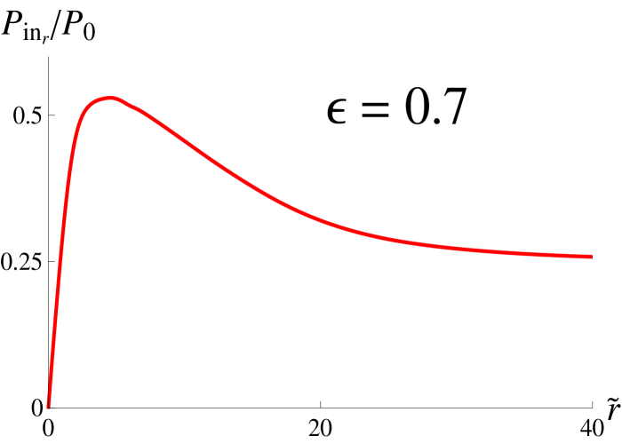
Figure 8: Color online. $P_{in_{r}}/P_{0}$ vs $\tilde{r}$ for $\epsilon=0.7$. Note the the slope is negative for $\tilde{r}\gtrsim 4$, idicating that power is exiting medium 2 at such radii.

V Summary

We have looked at power flow in the problem of a dipole radiating above a metallic or dielectric half-space in the limit that the imaginary part of the permittivity of the metal or dielectric is much less than unity. In particular, we have tried to emphasize the somewhat unexpected results that were obtained for the metallic half-space when the dipole’s emission frequency is close to but below the surface plasmon resonance frequency, corresponding to the real part of the permittivity slightly less than $-1.$ For a dielectric with $\epsilon>1$, there is an enhancement of power flow owing to the fact that the near field of the dipole can couple to propagating modes, but no surprises insofar as the direction of energy flow. On the other hand, for $0<\epsilon<1,$ there can be flow out of the dielectric for sufficiently large radii, a result reminiscent of the Goos-Hänchen effect.

Perhaps the best summary is represented by the series of graphs (Figs. 9-14) showing the Poynting vector (in arbitrary units) as a function of $\tilde{r}$ and $\tilde{z}$ for a dipole located at $\tilde{d}=0.5$. Figure 9 corresponds to a dipole emitting in free space, where the Poynting vector points radially outwards from the dipole.

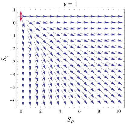
Figure 9: Color online. Components of the Poynting vector (in arbitrary units) for a dipole radiating in vacuum. The results are scaled such that the magnitude of the Poynting vector is constant at all points. The position of the dipole is indicated by the double-arrow.

In this and all other figures in this section, the results are scaled by a factor

$$s=\frac{\left[\tilde{\rho}^{2}+\left(\tilde{z}-\tilde{d}\right)^{2}\right]^{2}}{\tilde{\rho}^{2}}.$$ (68)

With this scaling factor the magnitude of the Poynting vector for a dipole radiating in free space is constant scaling .

The case of a metal with $\epsilon=-1.1+0.001i$ is illustrated in Fig. 10. It is seen that most of the energy is converted into lateral, evanescent waves that propagate radially outwards above the interface and radially inwards below the interface. There is a normal flow of energy into medium 2 for large $\tilde{\rho}$, but this not easily seen since the radial component of the Poynting vector is much larger than the $z$ component at such points. Figure 11 shows analogous results for $\epsilon=-0.9$, a value that in the Drude model that corresponds to a frequency in the gap of the dispersion curves between the surface plasmon and plasma frequencies. For this value of $\epsilon$, a plane wave impinging on the interface at any angle of incidence would be totally reflected, but there would be lateral waves in medium 2 for an angle of incidence other than zero. In the case of the dipole emitter, the net (integrated) energy flow into the surface vanishes, but there can be interesting flow patterns into and out of the the surface at different radii, such as that shown in Fig. 11. The magnitude of the Poynting vector in this and subsequent figures is thousands of times smaller than those in Fig. 10. If $\epsilon$ is increased to a value such that $-0.525\lesssim\epsilon<0$, the direction of the vortex flow seen in Fig. 11 changes direction; that is, power exits rather than enters the metal near $\tilde{\rho}=0$. For $\epsilon\sim 0$, the amplitude of the evanescent waves approaches zero (see below). The case of a dielectric having $\epsilon=4$ is shown in Fig. 12. For this value of $\epsilon$, the maximum angle of refraction for incident plane waves is $30^{\circ};$ for the dipole emitter, the near field is converted to waves in medium 2 that propagate with angles of refraction greater than this value. The feature we described as reminiscent of that seen in the Goos-Hänchen effect is seen in Fig. 13 for $\epsilon=0.7.$ There are evanescent waves in the dielectric leading to power flow out of the dielectric for $\tilde{\rho}\gtrsim 4$. Finally, in Fig. 14, we model a medium having negative refraction by taking $\epsilon=-1.1+0.001i$ and $\mu=-1$. The features of negative refraction are readily observed in the figure as rays propagate into medium 2 but with ”negative” angles of refraction for $1.5\lesssim\tilde{\rho}<3$.

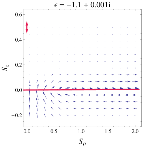
Figure 10: Color online. Components of the Poynting vector (in arbitrary units) for $\epsilon=-1.1+.001i$. The results are scaled as in Fig. 9.

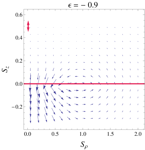
Figure 11: Color online. Components of the Poynting vector (in arbitrary units) for $\epsilon=-0.9$. The results are scaled as in Fig. 9.

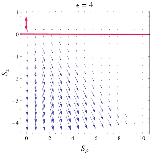
Figure 12: Color online. Components of the Poynting vector (in arbitrary units) for $\epsilon=4$. The results are scaled as in Fig. 9.

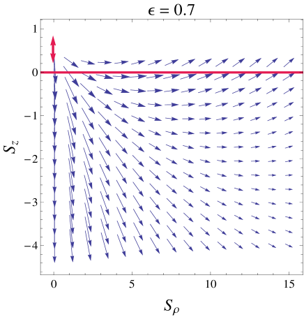
Figure 13: Color online. Components of the Poynting vector (in arbitrary units) for $\epsilon=0.7$. The results are scaled as in Fig. 9.

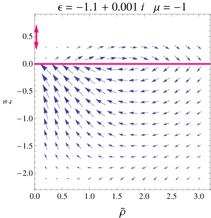
Figure 14: Color online. Components of the Poynting vector (in arbitrary units) for $\epsilon=-1.1+0.001i$ and $\mu=-1$. The results are scaled as in Fig. 9.

All the calculations have been carried out for a dipole driven at constant amplitude and for $0\leq\epsilon_{i}\ll 1$. It is not too difficult to understand the role played by loss in medium 2 as the value of $\epsilon_{i}$ is increased. If there is no contribution from surface plasmons, the dominant effect of increased loss is an increase in the rate of Joule heating. As such, the power transmitted into the medium increases with increasing $\epsilon_{i}$ (up to a value of $\epsilon_{i}$ of order 1 to 10, after which it decreases); the increased power is dissipated as Joule heat. On the other hand, for $\epsilon_{r}<-1$ and $\mu>0$, the change in transmitted power is controlled by two competing mechanisms. On the one hand there is an increase in the transmitted power with increasing $\epsilon_{i}$ owing to Joule heating, but there is a decrease in transmitted power resulting from the fact that the surface plasmon contribution decreases with increasing $\epsilon_{i}$. As a consequence, for frequencies slightly below the surface plasmon resonance frequency, the transmitted power decreases with increasing $\epsilon_{i}$; however as the frequency is reduced such that $\epsilon_{r}\lesssim 1.3$, the increase in Joule heating is dominant and the transmitted power increases with increasing $\epsilon_{i}$. For a real metal such as silver and a dipole radiating at optical frequencies, the incident field frequency is well below the surface plasmon resonance frequency, such that $\epsilon\approx-17+0.5i$; in this limit $P_{in}/P_{0}=4.0$; moreover, the value of $S_{\rho}$ just above the metal is roughly 17 times its value just below the surface, owing to the boundary condition given in Eq. (23b).

An interesting situation occurs for $-1<\epsilon_{r}<0$. In this case there is no net transmitted power for $\epsilon_{i}=0$, so the net transmitted power increases with increasing $\epsilon_{i}$ as a result of Joule heating. In addition, the radial component of the time-averaged Poynting vector near the surface can be amplified significantly for small values of $\epsilon_{i}$ if $\tilde{\rho}<1$. Setting $\mathbf{E}_{1z}(z=0)\mathbf{H}_{1\phi}^{\ast}(z=0)=A+iB$, we find from Eq. (23b) that

$$\frac{S_{1\rho}(z=0)}{S_{2\rho}(z=0)}=\epsilon_{r}-\epsilon_{i}\frac{B}{A}$$ (69)

If $\left|B/A\right|\gg 1,$ the second term in this expression can be important, even if $\epsilon_{i}\ll 1$.

Another interesting limit is that of zero index materials nim . In the Drude model, $\epsilon\sim 0$ if $\omega=\omega_{p}$ and there are no losses. For the vertical dipole considered in this paper, if $\epsilon=0$, all the results are independent of $\mu$. In this limit, the magnetic field (and the Poynting vector) in the metal vanishes. Since $\mathbf{H}=0$ in the metal, the curl of the electric field vanishes in the metal. As such, the electric field which penetrates into the metal has the characteristics of a static, conservative field. The situation is somewhat analogous to that encountered in the scattering of a matter wave by a potential step when the energy of the particle is slightly below the step height. In that case the wave function penetrates far into the classically forbidden region, but the probability current density vanishes in the classically forbidden region. If we had considered a horizontal dipole with $\epsilon=\mu=0$, we would have found that the curl of $\mathbf{E}$ and $\mathbf{H}$ both vanish in the medium, but the Poynting vector no longer vanishes since both $\mathbf{E}$ and $\mathbf{H}$ are non-zero in the medium (in contrast to both $\mathbf{B}$ and $\mathbf{D}$, which do vanish). Although the integrated flow of energy into the medium equals zero, the $z-$component of the Poynting vector at the surface is not equal to zero, but is a function of $\rho$ and $\phi$.

To see how the decay properties of an atom are modified by the surface, it would be better to look at the dynamics of the decay process for a dipole prepared with some initial displacement or velocity. This is a more difficult problem than that of the dipole driven at constant amplitude, but might be tractable if retardation effects are neglected insofar as they affect the amplitude of the dipole during its decay. In the case of a metal we could expect a large enhancement of the decay rate of the dipole if it can couple to surface plasmon modes.

PRB is pleased to acknowledge helpful discussions with G. Barton, G. W. Ford, R. Merlin, P. Milonni, M. Revsen, and D. Steel. This work was funded in part by the Air Force Office of Scientific Research (AFOSR, Dr. Gernot Pomrenke, Grant FA9550-13-1-0003), the National Science Foundation Atomic, Molecular and Optical Physics (NSF-AMOP) and the Engineering Research Center for Integrated Access Networks (ERC-CIAN, Award EEC-0812072). SZ would like to acknowledge the support of the Department of Energy (DOE) through the Office of Science Graduate Fellowship (SCGF) made possible in part by the American Recovery and Reinvestment Act of 2009, administered by ORISE-ORAU under contract no. DE-AC05-06OR23100.

VI Appendix: Asymptotic evaluation of various integrals

VI.1 $P_{in}$ and $J$ for $\mu=1$, $\epsilon_{r}<-1$ and $\epsilon_{i}\ll 1$

If we take $\mu=1$, $\epsilon_{i}=0$ and $\epsilon_{r}<-1$, the integrand in Eq. (29) for $P_{in}$ is purely real (recall that $\ell_{2}=-i\sqrt{\epsilon-u^{2}}=\sqrt{u^{2}+\left|\epsilon_{r}\right|}$ in this limit), but the integral diverges; as a consequence, the entire expression for $P_{in}$ is ill-defined. However, for an infinitesimal value of $\epsilon_{i}$, the integral no longer diverges and the integrand has a sharp maximum at

$$\ell_{2}(u_{0})=-\epsilon\ell_{1}(u_{0})$$ (70)

or

$$u_{0}=\sqrt{\frac{\epsilon_{r}}{\epsilon_{r}+1}}.$$ (71)

The region of integration about $u=u_{0}$ provides the dominant contribution to $P_{in}$ and this contribution is zeroth order in $\epsilon_{i}$. Thus, the expression for $P_{in}$ can be approximated as

$$P_{in}\sim\frac{k_{1}^{3}p^{2}\omega\epsilon_{r}^{2}}{\epsilon_{1}}\operatorname{Re}\left\{\left(\frac{ie^{-2\ell_{1}(u_{0})\tilde{d}}}{\epsilon}\right)\int_{0}^{\infty}\frac{\ell_{2}\left(\epsilon,u_{0}\right)u_{0}^{3}}{\left|K(\epsilon_{r},u_{0})\right|^{2}\left[\left|\left(u-u_{0}\right)^{2}+\left(\epsilon_{i}^{\prime}/2\right)\right|^{2}\right]}du\right\},$$ (72)

where

$$K(\epsilon,u)=\frac{u}{\sqrt{u^{2}-\epsilon}}+\frac{\epsilon u}{\sqrt{u^{2}-1}},$$ (73)

$$u_{p}=u_{0}-i\epsilon_{i}^{\prime}/2,$$ (74)

and (to order $\epsilon_{i}$)

$$\epsilon_{i}^{\prime}=\epsilon_{i}/[\left|\epsilon_{r}\right|^{1/2}\left(\left|\epsilon_{r}\right|-1\right)^{3/2}]$$ (75)

By extending the integral to $-\infty$, one obtains

$$P_{in}\sim\frac{k_{1}^{3}p^{2}\omega\epsilon_{r}^{2}e^{-2\ell_{1}(u_{0})\tilde{d}}}{\epsilon_{1}}\frac{2\pi}{\epsilon_{i}^{\prime}}\operatorname{Re}\left\{\left(\frac{i}{\epsilon}\right)\frac{\ell_{2}\left(\epsilon,u_{0}\right)u_{0}^{3}}{\left|K(\epsilon_{r},u_{0})\right|^{2}}\right\}.$$ (76)

We now use the fact that

$$\ell_{2}\left(\epsilon,u_{0}\right)=\sqrt{\frac{\epsilon^{2}}{\epsilon+1}};\text{ \ \ \ \ \ \ }\epsilon=\epsilon_{r}+i\epsilon_{i}$$ (77)

and

$$K(\epsilon_{r},u_{0})\equiv K(u_{0})=-\frac{\left(\left|\epsilon_{r}\right|^{2}-1\right)}{\sqrt{\left|\epsilon_{r}\right|}}.$$ (78)

to arrive at

$$P_{in}\sim\frac{k_{1}^{3}p^{2}\omega\pi\left|\epsilon_{r}\right|^{3}e^{-2\sqrt{\frac{1}{\left|\epsilon_{r}\right|-1}}\tilde{d}}}{\epsilon_{1}\left(\left|\epsilon_{r}\right|-1\right)^{5/2}\left(\left|\epsilon_{r}\right|+1\right)}.$$ (79)

Following the same procedure used above to calculate $P_{in}$, the Joule heating $J$ given by Eq. (32) is evaluated as

$$J =\frac{\epsilon_{i}\omega k_{1}^{3}p^{2}4\left|\epsilon\right|^{2}}{4\epsilon_{1}\left|\epsilon\right|^{2}}e^{-2\ell_{1}(u_{0})\tilde{d}}u_{0}^{3}\frac{\left(\left|\ell_{2}(u_{0})\right|^{2}+u_{0}^{2}\right)}{2\ell_{2}(\epsilon,u_{0})K(u_{0})^{2}}\frac{\pi}{\left(\epsilon_{i}^{\prime}/2\right)}$$

$$=\frac{k_{1}^{3}p^{2}\omega\pi\left|\epsilon_{r}\right|^{3}e^{-2\sqrt{\frac{1}{\left|\epsilon_{r}\right|-1}}\tilde{d}}}{\epsilon_{1}\left(\left|\epsilon_{r}\right|-1\right)^{5/2}\left(\left|\epsilon_{r}\right|+1\right)}.$$ (80)

VI.2 $P_{rad}$, and $J_{r}$ for $\mu=1$, $\epsilon_{r}<-1$, $\epsilon_{i}\ll 1$, and $\tilde{r}\gg 1$

To evaluate Eq. (36) for $P_{rad}$ in the limit that $u_{0}\tilde{r}\gg 1$, we can replace the Bessel functions appearing in Eq. (36) by their asymptotic forms for large argument and keep only the outgoing waves (Hankel functions of the first kind) if $u_{0}\tilde{r}\gg 1.$ (the two forms of the integrals give about the same results - the contributions from $u\ll 1$ differ since the use of outgoing Hankel functions is not justified in that case, but the corrections from this region are small). Thus, for $u_{0}\tilde{r}\gg 1$, we can set

$$P_{rad}(asy)\sim\frac{k_{1}^{3}p^{2}\omega}{4\epsilon_{1}}\left(\frac{2}{4\pi}\right)\operatorname{Re}\left\{\begin{array}[c]{c}\left(-\frac{i}{\epsilon}\right)\int_{0}^{\infty}du\int_{0}^{\infty}du^{\prime}\frac{u^{5/2}}{\ell_{1}(u)}e^{i\left(\tilde{r}u-\pi/4\right)}e^{-\ell_{1}(u)\tilde{d}}f_{2}(u)\\ \times\frac{u^{\prime 3/2}}{\ell_{1}^{\ast}(u^{\prime})}e^{-\ell_{1}^{\ast}(u^{\prime})\tilde{d}}f_{2}^{\ast}(u^{\prime})e^{-i\left(\tilde{r}u^{\prime}-3\pi/4\right)}\frac{1}{\ell_{2}(u)+\ell_{2}^{\ast}(u^{\prime})}\end{array}\right\},$$ (81)

where ”asy” stands for ”asymptotic.” We now evaluate all factors, except the exponentials in $\tilde{\rho},$ at $u=u_{0}$ or $u^{\prime}=u_{0}$. In this manner we obtain

$$P_{rad}(asy)\sim\frac{k_{1}^{3}p^{2}\omega}{4\epsilon_{1}}\left(\frac{2}{4\pi}\right)\frac{4\epsilon_{r}u_{0}^{4}e^{-2\ell_{1}(u_{0})\tilde{d}}}{2\ell_{2}(\epsilon_{r},u_{0})K^{2}(u_{0})}\left|\int_{0}^{\infty}du\frac{e^{i\tilde{r}u}}{u-u_{0}-i\epsilon_{i}^{\prime}/2}\right|^{2}.$$ (82)

Finally by extending the integral to $-\infty$, we arrive at

$$P_{rad}(asy) \sim\frac{k_{1}^{3}p^{2}\omega}{4\epsilon_{1}}\left(\frac{2}{4\pi}\right)\frac{4\epsilon_{r}u_{0}^{4}e^{-2\ell_{1}(u_{0})\tilde{d}}}{2\ell_{2}(\epsilon_{r},u_{0})K^{2}(u_{0})}4\pi^{2}e^{-\epsilon_{i}^{\prime}\tilde{r}}$$

$$=-\frac{k_{1}^{3}p^{2}\omega\pi e^{-2\sqrt{\frac{1}{\left|\epsilon_{r}\right|-1}}\tilde{d}}e^{-\epsilon_{i}^{\prime}\tilde{r}}}{\epsilon_{1}}\frac{\left|\epsilon_{r}\right|^{3}}{\left(\left|\epsilon_{r}\right|-1\right)^{7/2}\left(\left|\epsilon_{r}\right|+1\right)^{2}}.$$ (83)

The integrals in Eq. (41) have their major contributions for $u\approx u^{\prime}\approx u_{0}.$ In the limit of large $\tilde{r}$, we can use Eq. (26) to obtain an asymptotic expansion, as we did for the radial power. Even though small values of $\tilde{\rho}$ enter the integration, their contribution is relatively small for large $\tilde{r}$. Evaluating integrals in Eq. (41) as we did for the radial term, we find

$$J_{r}(asy) \sim\frac{\epsilon_{i}\omega k_{1}^{3}p^{2}}{\epsilon_{1}}\int_{0}^{\tilde{r}}\tilde{\rho}d\tilde{\rho}\int_{-\infty}^{0}d\tilde{z}\left(\frac{2}{4\pi}\right)\frac{u_{0}^{3}e^{-2\ell_{1}(u_{0})\tilde{d}}e^{2\ell_{2}(\epsilon_{r},u_{0})\tilde{z}}}{K^{2}(u_{0})}$$

$$\times\left[\ell_{2}(\epsilon_{r},u_{0})^{2}+u_{0}^{2}\right]\left|\int_{-\infty}^{\infty}du\frac{e^{i\tilde{r}u}}{u-u_{0}-i\epsilon_{i}^{\prime}/2}\right|^{2}$$

$$=\frac{\omega k_{1}^{3}p^{2}}{\epsilon_{1}}\frac{\pi u_{0}^{3}e^{-2\ell_{1}(u_{0})\tilde{d}}e^{2\ell_{2}(\epsilon_{r},u_{0})\tilde{z}}}{\ell_{2}(\epsilon_{r},u_{0})K^{2}(u_{0})\left(\epsilon_{i}^{\prime}/\epsilon_{i}\right)}\left[\ell_{2}(\epsilon_{r},u_{0})^{2}+u_{0}^{2}\right]\left(1-e^{-\epsilon_{i}^{\prime}r}\right)$$

$$=\frac{\pi\omega k_{1}^{3}p^{2}}{\epsilon_{1}}\frac{\left|\epsilon_{r}\right|^{3}e^{-2\sqrt{\frac{1}{\left|\epsilon_{r}\right|-1}}\tilde{d}}}{\left(\left|\epsilon_{r}\right|-1\right)^{5/2}\left(\left|\epsilon_{r}\right|+1\right)}\left(1-e^{-\epsilon_{i}^{\prime}\tilde{r}}\right).$$ (84)

References

- (1) A. Sommerfeld, Partial Differential Equations in Physics, (Academic Press, New York, 1949), Chap. 6.
- (2) See, for example; A. Baños, Dipole Radiation in the Presence of a Conducting Half-Space (Pergamon Press, Oxford,1966), and references therein; R. W. P. King, M. Owens, and T. T. Wu, Lateral Electromagnetic Waves (Springer-Verlag, New York, 1992), and references therein; D. Margetis and T. T. Wu, J. Math. Phys. 42, 713-745 (2001), and references therein; B. Ung and Y. Sheng, B. Ung and Y. Sheng, Optics Express, 16, 9073-9086 (2008).
- (3) R. R. Chance, A. Prock, and R. Silbey, in Advances in Chemical Physics, edited by I. Prigogine and S. A. Rice (Wiley, New York, 1978) Vol. 37, pps 1-65.
- (4) G. W. Ford and W. H. Weber, Phys. Reps. 113, 195-287.
- (5) See also, for example, H. Morawitz and M. R. Philpott, Phys. Rev. B 10, 4863-4868 (1974); J. E. Sipe, Surface Science 105, 489-504 (1981); J. M. Wylie an J. E. Sipe, Phys. Rev. A 30, 1185-1193 (1984); W. L. Barnes, J. Mod. Opt. 45, 661-699 (1998), and references therein.
- (6) See, for example, J. M. Pitarke, V. M. Silkin, E. V. Chulkov, and P. M. Echenique, Rep. Prog. Phys. 70, 1-87 (2007), and references therein.
- (7) W. Lukosz and R. E. Kunz, J. Opt. Soc. Amer. 67, 1607-1615 (1977); ibid. 1615-1619.
- (8) L. Novotny, J. Opt. Soc. Amer. A 14, 91-104 (1997). (1977)
- (9) L. Novotny and B. Hecht, ”Principles of Nano-Optics,” (Cambridge Univ. Press, New York, 2006) Chap. 10.
- (10) After this paper was submitted, an article appeared [H. F. Arnoldus and M. J. Berg, J. Mod. Opt. 62, 244 (2015)] in which the energy flow was calculated for emission from a dipole located above a dielectric slab (the slab has interfaces with two dielectrics, one of which contains the dipole). The permittivities are all taken to be real, so there are no contributions from surface plasmons; however, when the permittivity of the slab is less than that of the medium in which the dipole is located, patterns similar to those shown in Fig. 13 are found and a vortex pattern in the slab can also occur. PRB would like to thank M. Revsen for pointing out this reference.
- (11) See for example, P. N. Stavrinou and L. Solymar, Opts. Comm. 206, 217 (2002); H. F. Schouten, T. D. Vissar, D. Lenstra, and H. Blok, Phys. Rev. E 67, 036608 (2003); H. F. Schouten, T. D. Vissar, and D. Lenstra, J. Opt. B: Semiclass. Opt. 6, S404 (2004); J. Wuenschell and H. K. Kim, Opt. Exp. 14, 10000 (2006).
- (12) See for example, V. G. Veselago, Sov. Phys. Uspekhi 10, 509 (1968); D. R. Smith and N. Kroll, Phys. Rev. Lett. 85, 2933 (2000); J. B. Pendry, Phys. Rev. Lett. 85, 3966 (2000); R. W. Ziolkowski and E. Haymen, Phys. Rev. E 64, 056625 (2001); R. A. Shelby, D, R. Smith, and S. Schultz, Science 292, 77 (2001): J. B. Pendry and D. R. Smith, Phys. Today 57, 37 (2004); R. Merlin, App. Phys. Lett. 84, 1290 (2004); J. B. Pendry, Cont. Phys. 45, 191 (2004); A. Petrin, in Wave Propagation in Materials for Modern Applications, edited by A. Petrin (InTech, Croatia, 2010) Chap. 7; Y. Ra’di, S. Nikmehr, and S. Hosseinzadeh, Prog. Electro. Rsch. 116, 107 (2011); J. T. Costa, M. G. Silveirinha, and Alù, Phys. Rev. B 83, 165120 (2011).
- (13) See for example, W. T. Chen, P. C. Wu, C. J. Chen, H.-Y. Chung, Y.-F. Chau, C.-H. Kuan, and D. P. Tsai, Opt. Exp. 18, 19665 (2010).
- (14) See, for example, D. E. Chang, A. S. Sørensen, P. R. Hammer, and M. D. Lukin, Phys. Rev. B 76, 035420 (2017); L. Novotny, Phys. Rev. Lett. 98, 266802 (2007); V. Giannini, J. A. Sánchez-Gil, O. L. Muskens, and J. G. Rivas, J. Opt. Soc. Am. B 26, 1569 (2009); N. Meinzer, M. Ruther, S. Linden, C. M. Soukoulis, G. Khitrova, J. Hendrikson, J. D. Olitsky, H. M. Gibbs, and M. Wegener, Opt. Exp. 18, 24140 (2010); J.-J. Greffet, M. Laroche, and F. Marquier, Phys. Rev. Lett. 105, 117701 (2010); A. G. Curto, G. Volpe, T. H. Taminiau, M. P. Kreuzer, R. Quidant, and N. F. van Hulst, Science 329, 930 (2010; L. Novotny and N. van Hulst, Nat. Phot. 5, 83 (2011); M. Husnik, J. Niegemann, K. Busch, and M. Wegener, Opt. Lett. 38, 4597 (2013); N. Kumar, thesis, Univ. Cal. Berkeley (2013), available at http://www.eecs.berkeley.edu/Pubs/TechRpts/2013/EECS-2013-107.html; A Delga, J. Feist, J. Bravo-Abad, and F. J. Garcia-Vidal, Phys. Rev. Lett. 112, 253601 (2014); G. M. Akselrod, C. Argyropoulos, T. B. Hoang, C. Ciracì, C. Fang, J. Huang, D. R. Smith & M. H. Mikkelsen, Nat. Phot. 8, 835 (2014).
- (15) For arbitrary permittivity and permeability, expressions for the electric field vectors are given in V. K. Ivanov, A. O. Silin, and O. M. Stadnyk, 2013 International Kharkov Symposium on Physics and Engineering of Microwaves, Millimeter and Submillimeter Waves (MSMW), Kharkov, Ukraine, pp. 467-469.
- (16) Chance et al. sil take the electric field in a medium having permittivity as whereas Sommerfeld takes it as . As a consequence the boundary conditions on the Hertz vector should be given by ; for Chance et al., whereas they are ; for Sommerfeld. Chance et al. use Sommerfeld’s boundary conditions which lead to an incorrect equation for the fields in medium 2 [their Eq. (2.14)]. The factor of should be deleted from that equation; otherwise the component of the Poynting vector would not be continuous across the interface. Chance et al. do not calculate the fields in medium 2, so this error does not play a role in their results.
-
(17)
If , there is an additional loss
term. We can define an effective rate of Joule heating as
See, for example, J. D. Jackson, Classical Electrodynamics, Third Edition (Wiley, New York, 1999) Sec. 6.8. - (18) Since the scaling procedure involves division by , the Poynting vector can be artificially enhanced in regions near the axis (for ), even if its actual magnitude is small. This is especially the case when in such cases, the region near the axis is artificially suppressed for small . If we did not do this, the diagrams would be dominated by one or two arrows located near .
- (19) See, for example, M. Silveirinha and N. Engheta, Phys. Rev. Lett. 97, 157403 (2006); S. Liu, W. Chen, J. Du, Z. Lin, S. T. Chui, and C. T. Chan, Phys. Rev. Lett. 101, 157407 (2008); V. C. Nguyen, L. Chen, and K. Halterman, Phys. Rev. Lett. 105, 233908 (2010); X. Huang, Y. Lai, Z. H. Hang, H. Zheng, and C. T. Chan, Nature Mat. 10, 582 (2011); K. Zhang1, J. Fu, Li-Yi Xiao, Q. Wu, and Le-Wei Li, J. Appl. Phys. 113, 084908 (2013); X. Yu, H. Chen, H. Lin, J. Zhou, J. Yu, C. Qian, and S. Liu, Opt. Lett. 39, 4643 (2014).