Lindbladians for controlled stochastic Hamiltonians

Abstract

We construct Lindbladians associated with controlled stochastic Hamiltonians in weak coupling. This allows to determine the power spectrum of the noise from measurements of dephasing rates; to optimize the control and to test numerical algorithms that solve controlled stochastic Schrödineger equations. A few examples are worked out in detail.

1 The problem and the result

This article describes Lindbladians associated with controlled stochastic Hamiltonians in weak coupling. Controlled stochastic Hamiltonians arise in the context of “dynamical decoupling” and “coherent control” and are used to examine protocols for extending the coherence time of qubits [12, 9, 2].

Lindbladians in the weak coupling limit have been rigorously studied in [6, 13, 10, 4, 5, 18, 1, 16, 7] in the time independent setting. Recently, controls aimed at extending the coherence of qubits have been suggested in [12, 9] and periodically controlled Lindbladians have been studied in [2, 20]. However a careful derivation of the Lindbladians for the controlled stochastic evolutions and in particular Eq. (3.8) for general and in Eq. (1) for stationary control are new. This is also the case for the notion of effective control introduced in Appendix C.1 and some of the examples in section 4.

Consider the stochastic controlled Hamiltonian.

$$\underbrace{\left(\sum\xi_{\alpha}(t)H_{\alpha}\right)}_{weak~{}noises}+\underbrace{H_{c}(t)}_{control},$$ (1.1)

$H_{\alpha}$ are fixed Hermitian matrices representing independent and in general non-commuting sources of noise. $\xi_{\alpha}$ are stationary Gaussian random processes

$$\mathbb{E}\left(\xi_{\alpha}(t)\right)=0,\quad\mathbb{E}\left(\xi_{\alpha}(t)\xi_{\beta}(u)\right)=J_{\alpha\beta}\left({|t-u|}\right)\,.$$ (1.2)

with $J$ rapidly decreasing on a time scale $\tau$. We shall sometimes assume, w.l.o.g., that $J$ is a diagonal matrix (this can be achieved by a redefinition of $H_{\alpha}$). A spin in a magnetic field having fixed direction but noisy amplitude, often a good approximation [12, 9], is represented by a single term $\alpha$. The case where the direction of the field is also stochastic is modeled by several $\alpha$’s and gives rise to noise that is non-commutative (not been treated before.) $H_{c}$, a time-dependent (Hermitian) matrix, represents the control.

It is convenient to reformulate the problem in the interaction picture. Let

$$H^{I}_{\xi}(t)=\sum_{\alpha}\xi_{\alpha}(t)H^{I}_{\alpha}(t),\quad H^{I}_{\alpha}(t)=V^{*}(t)H_{\alpha}V(t)$$ (1.3)

where $V(t)$ is the unitary generated by the control $H_{c}(t)$,

$$H_{c}=i\dot{V}(t)V^{*}(t),\quad V(0)=\mathbbm{1}$$ (1.4)

Weak coupling parameter in the present context is defined by

$$\varepsilon^{2}={\tau\|\tilde{J}\|}\,\|H_{\alpha}\|^{2}\ll 1\quad\tilde{J}(\omega)=\int_{-\infty}^{\infty}e^{i\omega t}J(t)dt\geq 0$$ (1.5)

$\varepsilon$ is the phase acquired by the wave function during one correlation time (in the absence of control). There are several ways to think about weak coupling: If we think of $\|\tilde{J}\|,\tau=O(1)$ then weak coupling means what its names suggests, namely, that the noise is weak in the sense that $\|H_{\alpha}\|=O(\varepsilon)$. An alternate approach, which is also insightful, is to take $\|\tilde{J}\|,\|H_{\alpha}\|=O(1)$ and then weak coupling means short correlation time $\tau=O(\varepsilon^{2})$.

The noise affects the (average) state on the coarse grained time scale

$$s=\varepsilon^{2}t/\tau$$ (1.6)

Control problems are characterized by the rate of rotation of $H^{I}_{\alpha}(t)$. For example, when the control $H_{c}$ is time independent, (constant control), $\omega=\|H_{c}\|$ while for periodic Bang-Bang, where $H_{c}(t)$ is a (periodic) sequence of delta pulses, $\omega_{c}$ is the frequency of the bangs. This gives rise to a second dimensionless parameter $\omega_{c}\tau$. Our analysis of the weak coupling limit holds independently of $\omega_{c}\tau$. Dynamical decoupling requires however $\omega_{c}\tau\gtrsim 1$ where the time scale of the control, $\delta t=O(1/\omega_{c})$, is not resolved on the coarse grained time scale $s$.

By stationary controls we shall mean that $H^{I}_{\alpha}(t)$ has a finite number of Fourier coefficients. It is convenient to factor $\varepsilon$ so that the Fourier coefficients are $\tilde{H}_{\alpha}(\omega)$ are

$$H^{I}_{\alpha}(t)=\varepsilon\sum_{\omega\in F}\tilde{H}_{\alpha}(\omega)\,e^{i\omega t},\quad\tilde{H}_{\alpha}(\omega)=\tilde{H}^{*}_{\alpha}({-\omega})$$ (1.7)

$F$ a finite set.

When $\varepsilon\ll 1$ we shall show that the evolution is governed by (complete) positivity preserving Lindbladian

$$\frac{d\rho}{ds}={\cal L}_{\varepsilon}\rho$$ (1.8)

Moreover, we shall show that, in the case of stationary control, ${\cal L}_{\varepsilon}$ has a limit as $\varepsilon\to 0$ given by:

$${\cal L}=\sum_{\alpha}{\cal L}_{\alpha},\quad{\cal L}_{\alpha}={\mathbfcal H}_{\alpha}-{\mathbfcal D}_{\alpha}$$ (1.9)

with

$${\mathbfcal H}_{\alpha}\rho =\frac{i\tau}{4}\sum_{\omega\in F}\tilde{K}_{\alpha}(\omega)\big{[}[\tilde{H}_{\alpha}(\omega),\tilde{H}_{\alpha}^{*}(\omega)],\rho\big{]},$$

$${\mathbfcal D}_{\alpha}\rho =\frac{\tau}{8}\sum_{\omega\in F}\tilde{J}_{\alpha}(\omega)\big{[}\tilde{H}_{\alpha}(\omega),[\tilde{H}_{\alpha}^{*}(\omega),\rho]\big{]}$$ (1.10)

$\tilde{J}$ denotes Fourier transform and $K$ is the anti-symmetric partner of $J$ :

$$K_{\alpha}(u)=i\operatorname{sgn}(u)J_{\alpha}(u),$$ (1.11)

Note that $\tilde{K}(\omega)$ is real and $\tilde{K}(0)=0$. ${\mathbfcal H}_{\alpha}$ is a generator of unitary evolution since $[\tilde{H}_{\alpha}(\omega),\tilde{H}_{\alpha}^{*}(\omega)]$ is hermitian. Since $\tilde{J}(\omega)\geq 0$ ${\mathbfcal D}_{\alpha}\geq 0$ is a contraction, generating decoherence.

$$X_{j}\mapsto UX_{j}U^{*}=\sum R_{jk}X_{k}$$

with $U\in U(d)$ unitary and $R\in O(d^{2})$ orthogonal. An adapted basis is one where $\Gamma$ is a diagonal (positive) matrix. In this basis, ${\cal L}$ is manifestly a bona fide Lindbladian; i.e. complete positivity preserving.

Figure 1: The figure illustrates the self-averaging of the noise.

Remark 1.1.

The special form of ${\cal L}_{\alpha}$ reflects the fact that stochastic evolutions are unital: The fully mixed state $\rho\propto{\mathbbm{1}}$ is stationary.

Remark 1.2.

Eq. (1) can be used to determine $\tilde{J}$ from the measured rates $\gamma_{\alpha}$ [3, 14, 19, 15]. See the examples in section 4. Moreover, it implies that the optimal measurement time is $t=O(\tau/\varepsilon)$. To see this observe that repeated measurements of a projection $P$ in the state $\rho(t)$ generates a Poisson process with an average

$$Tr(\rho(t)P)=p(\gamma,t)$$

Given total allotted time $T$, an optimal estimator minimizes the standard deviation in $\gamma$. This fixes $t$ to be the minimizer of the sensitivity

$$S=\frac{\sqrt{tp(1-p)}}{|\frac{dp}{d\gamma}|}$$

Eq. (1) determines $\rho(t)$ for $t\geq\tau/\varepsilon$. For a depolarizing qubit

$$\rho(t)=e^{-\gamma t}P+(1-e^{-\gamma t})\mbox{$\frac{1}{2}$}\mathbbm{1},\quad p(\gamma,t)=\frac{1-e^{-\gamma t}}{2}$$

so $S$ takes its minimum at the left edge of the interval, $t=O(\tau/\varepsilon)$.

2 Some exact results

The Hamiltonian $H^{I}_{\xi}$ generates a stochastic unitary evolution $U_{\xi}$ given by

$${U}_{\xi}(t) =\left(e^{-i\int_{0}^{t}H^{I}_{\xi}(u)du}\right)_{T}$$ (2.1)

$$=\sum_{n=0}^{\infty}(-i)^{n}\int_{0\leq t_{1}<t_{2}<\dots<t_{n}\leq t}H_{\xi}(t_{n})dt_{n}\dots H_{\xi}(t_{1})dt_{1}$$

The time ordering, denoted by the subscript $T$ in the first line is defined explicitly in the second. More crucial to us is the super-operator ${\cal{U}}_{\xi}$ acting on states

$$\rho_{0}\mapsto\rho_{\xi}(t)={\cal{U}}_{\xi}\rho_{0}=U_{\xi}(t)\rho_{0}U_{\xi}^{*}(t)$$ (2.2)

The super-operator can be written similarly

$${\cal{U}}_{\xi}(t) =\left(e^{-i\int_{0}^{t}{\cal{H}}_{\xi}(s)ds}\right)_{T}$$ (2.3)

$$=\sum_{n=0}^{\infty}(-i)^{n}\int_{0\leq t_{1}<t_{2}<\dots<t_{n}\leq t}{\cal{H}}_{\xi}(t_{n})dt_{n}\dots\cal{H}_{\xi}(t_{1})dt_{1}$$

where the super-operators ${\cal{H}}$ acts by the adjoint action

$${\cal{H}}\rho=\big{(}ad[H]\big{)}\rho\equiv[H,\rho]$$ (2.4)

Note that $ad[H_{1}]ad[H_{2}]\neq ad[H_{1}H_{2}]$. Rather,

$$(ad[H_{1}]ad[H_{2}])(\rho)=({\cal{H}}_{1}{\cal{H}}_{2})(\rho)={\cal{H}}_{1}({\cal{H}}_{2}\rho)=[H_{1},[H_{2},\rho]]$$ (2.5)

We also need the fact that

$$ad\big{[}[A,B]\big{]}=\big{[}ad[A],ad[B]\big{]}$$ (2.6)

which follows from Jacobi’s identity.

The key object of this study is the (stochastic) averaged evolution

$$\rho_{0}\mapsto\mathbb{E}\left(\rho_{\xi}(t)\right)=\big{(}{\cal{U}}(t)\big{)}\rho_{0}$$ (2.7)

The super-operator ${\cal{U}}(t)$ is trace preserving, (completely) positivity preserving and unital (i.e. ${\cal{U}}\mathbbm{1}=\mathbbm{1}$), but, in general, not unitary or Markovian.

Recall that for Gaussian averages

$$\mathbb{E}\left(e^{i\phi}\right)=e^{-\mathbb{E}\left(\phi^{2}\right)/2}$$ (2.8)

It follows that for $\xi$ a stationary Gaussian process,

$${\cal{U}}(t) =\left(\exp\left(-\mbox{$\frac{1}{2}$}\int_{0}^{t}du\int_{0}^{t}\,dv\,{\cal{K}}(u,v)\right)\right)_{T}$$

$$=\left(\exp\left(-\int_{0}^{t}du\int_{0}^{u}\,dv\,{\cal{K}}(u,v)\right)\right)_{T}$$ (2.9)

where

$${\cal{K}}(u,v)=\mathbb{E}\left({\cal{H}}^{I}_{\xi}(u){\cal{H}}^{I}_{\xi}(v)\right)=\sum_{\alpha\beta}J_{\alpha\beta}(u-v){\cal{H}}^{I}_{\alpha}(u){\cal{H}}^{I}_{\beta}(v)$$ (2.10)

So far, no approximation has been made. However, the time ordering remains a major complication. For its precise meaning one can either go back to Eq. (2.3), or alternatively, see the discussion and graphical representation in Appendix A. There is no issue with time ordering in two cases: when $\xi$ is white noise and when the (interaction picture) Hamiltonian commute at different times. We examine these cases first.

2.1 White noise

White noise is the limit $\tau\to 0$ with $\tau J=O(1)$. By Eq. (1.5) this corresponds to $\varepsilon\propto\sqrt{\tau}\to 0$. Not surprisingly, the reduction of white noise to Lindblad evolution is exact. Since $J_{\alpha\beta}(t)=J_{\alpha\beta}\delta(t)$ we have

$${\cal{U}}(t) =\left(\exp\left(\int_{0}^{t}du\ {\cal L}(u)\right)\right)_{T}$$ (2.11)

with

$${\cal{L}}(t)=-\frac{1}{2}\sum_{\alpha\beta}J_{\alpha\beta}{\cal{H}}^{I}_{\alpha}(t){\cal{H}}^{I}_{\beta}(t)$$ (2.12)

Since ${\cal L}$ and ${\cal{H}}^{I}$ have the same time argument $t$, we may use the definition of time-ordering in Eq. (2.3) with ${\cal{H}}_{\xi}\mapsto{\cal L}$, to conclude that ${\cal L}$ is the generator of ${\cal{U}}$. The Lindbladian reduces to:

$${\cal{L}}_{t}\rho=-\frac{1}{2}\sum_{\alpha\beta}J_{\alpha\beta}\big{[}{H}^{I}_{\alpha}(t),[{H}^{I}_{\beta}(t),\rho]\big{]}$$ (2.13)

The result is exact. Since $H_{\alpha}(t)$ are unitarily related for different $t$ it follows that the family ${\cal L}_{t}$ is unitarily related and hence isospectral. In particular, the instantaneous dephasing rates are independent of the control $V(t)$. This could be anticipated since to affect the dephasing rates, the control must be at least as fast as the noise correlations.

2.2 Commutative case

In general, it is difficult to extract a generator of the evolution from Eq. (2) because of the time ordering. In the commutative case this is not an issue and the generator of the evolution follows from Eq. (2.10). Let us denote

$${\cal{G}}(t)=-\int_{0}^{t}\,du\,{\cal{K}}(t,u)_{T} =-\sum_{\alpha}\int_{0}^{t}duJ_{\alpha\beta}(t-u)\left({\cal{H}}^{I}_{\alpha}(t){\cal{H}}^{I}_{\beta}(u)\right)_{T}$$ (2.14)

We then have

$${\cal{U}}(t) =\left(\exp\left(\int_{0}^{t}du\ {\cal{G}}(u)\right)\right)_{T}$$ (2.15)

Of course, in the commutative case the index $T$ is redundant. Now although ${\cal{G}}$ is an exact generator, it is not in general of Lindblad form. More precisely, it may fail to satisfy positivity at short times as the following example shows.

Example 2.1 (Commutative case).

The commutative case arises, for example, when the (interaction picture) noise has a stochastic amplitude but a fixed “direction”, i.e. when

$$H^{I}_{\xi}(t)=\xi(t)H_{0}$$

Since $H^{I}_{\xi}(t)$ is a commuting family, Eq. (2.15) is exact and the generator of the evolution is

$${\cal{G}}(t)\rho=-\frac{\gamma(t)}{2}{\cal{H}}_{0}{\cal{H}}_{0}\rho=-\frac{\gamma(t)}{2}[H_{0},[H_{0},\rho]],,$$ (2.16)

The “dephasing rate” $\gamma(t)$ is given by

$$\gamma(t)=2\int_{0}^{t}duJ(t-u)=2\int_{0}^{t}duJ(u)$$ (2.17)

Although $\gamma(0)\geq 0$ for very short times (since $J(0)>0$), $\gamma(t)$ may be negative for $t=O(\tau)$ as in Fig. 2. In these cases ${\cal{G}}(t)$ does not generate a contraction for all times. This reflects the fact that the evolution is not strictly Markovian. At longer times, $t\gg\tau$, one always has $\gamma(t)>0$ (since $\tilde{J}(0)\geq 0$).

Positivity is regained in the weak coupling limit. Here it is convenient to consider the limit in the sense of short correlation time so $\tau=\varepsilon^{2}$. We get from Eqs. (1.6,1.8)

$${\cal L}={\cal{G}},\quad(\tau=\varepsilon^{2})$$ (2.18)

In the limit $\varepsilon\to 0$, we get for $s>0$,

$${\cal L}\rho=-\frac{\tilde{J}(0)}{2}[H_{0},[H_{0},\rho]],$$ (2.19)

with time independent positive dephasing rate:

$$\quad 0<\tilde{J}(0)=\int_{-\infty}^{\infty}J(u)du=\lim_{\varepsilon\to 0}2\tau\int_{0}^{s/\varepsilon^{2}}J(u\tau)du$$ (2.20)

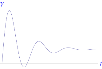
Figure 2: The figure shows $\gamma(t)$ for $J(t)=e^{-|t|}\cos 4t$ with $\gamma<0$ near the first minimum.

3 Weak coupling

Our aim is to obtain an approximate generator that is valid for small nonzero $\varepsilon$. The first step is to show that ${\cal{G}}$ defined in Eq. (2.14) remains an approximate generator in the noncommutative case . More precisely, moving the time ordering $T$ in the exact formula Eq. (2) into the exponential, comes with the penalty:

$${\cal{U}}(t) =\left(\exp\left(-\mbox{$\frac{1}{2}$}\int_{0}^{t}du\int_{0}^{t}\,dv\,{\cal{K}}(u,v)\right)\right)_{T}$$

$$=\exp\left(\int_{0}^{t}du\,{\cal{G}}(u)\right)_{T_{u}}+O\left(\frac{\varepsilon^{4}t}{\tau}\right)$$ (3.1)

Here $T_{u}$ denotes time ordering with respect to the integration variable $u$. This differs from the usual time ordering defined with respect to the argument of the hamiltonian. The error term results from the inequivalence of the two types of ordering. It is proportional to $t$ and hence is cumulative. It reflects the non-commutativity of the Hamiltonian at different times (there is no error in the commmutative case as we have seen in section 2.2). In particular, on the coarse grained time scale $s=O(1)\Leftrightarrow t=O(\tau/\varepsilon^{2})$ the error is $O(\varepsilon^{2})$. We justify this estimate in Appendix A.

As we have seen (again in section 2.2) ${\cal{G}}$ may not be a Lindbladian. Our next step is to show that within the framework of weak coupling, ${\cal{G}}$ is close to a generator that is of the Lindbladian form up to an $O(\varepsilon^{2})$ error.

To show this we introduce a useful representation of the noise $\xi$ in terms of white noises $W_{\alpha}$ :

$$\xi_{\alpha}(t)=\int_{-\infty}^{\infty}du\,j_{\alpha\beta}(t-u)W_{\beta}(u)$$ (3.2)

(summation implied) where

$$\mathbb{E}\left(W_{\alpha}(t)\right)=0,\quad\mathbb{E}\left(W_{\alpha}(t)W_{\beta}(u)\right)=\delta_{\alpha\beta}\delta(t-u)$$ (3.3)

There is freedom in defining $j$ which allows us to assume, w.l.o.g., that its Fourier transform is non-negative, $\tilde{j}(\omega)\geq 0$. $J$ is then the convolution of $j$ with itself:

$$J_{\alpha\beta}(u-v)=\int_{-\infty}^{\infty}dw\,j_{\alpha\gamma}(u-w)j_{\beta\gamma}(v-w)$$ (3.4)

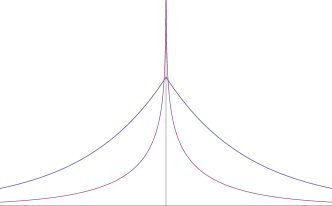
Figure 3: $J(t)=e^{-|t|}$ and the corresponding $j(t)=K_{0}(|t|)$, a Bessel function. $j$ is narrower than $J$.

With this notation in place we first note the identity

$$\left(\int_{0}^{t}dv\int_{0}^{t}du\,{\cal{K}}(u,v)\right)_{T} =\left(\int_{0}^{t}dv\int_{0}^{t}duJ_{\alpha\beta}(u-v){\cal{H}}^{I}_{\alpha}(u){\cal{H}}^{I}_{\beta}(v)\right)_{T}$$

$$=\sum_{\gamma}\int_{-\infty}^{\infty}\,dw\,\left(\int_{0}^{t}\,du\,j_{\alpha\gamma}(w-u){\cal{H}}_{\alpha}^{I}(u)\right)^{2}_{T}$$ (3.5)

which follows from Eq. (3.4).

The second step is the claim that we can interchange the limits of the $dw$ and $du$ integration in Eq. (3) up to a small error, i.e.

$$\int_{-\infty}^{\infty}\,dw\,\left(\sum_{\alpha}\int_{0}^{t}\,du\,j_{\alpha\gamma}(w-u){\cal{H}}^{I}_{\alpha}(u)\right)^{2}_{T}=\int_{0}^{t}\,dw\,\left({\cal{D}}_{\gamma}(w)\right)^{2}_{T}+O(\varepsilon^{2})$$ (3.6)

where

$${\cal{D}}_{\gamma}(w)=\frac{1}{2}\sum_{\alpha}\int_{-\infty}^{\infty}du\,j_{\alpha\gamma}(w-u){\cal{H}}^{I}_{\alpha}(u)$$ (3.7)

This follows from the fact that $j(u)$ is localized near the origin on a time scale $O(\tau)$. It is clear that the main contribution to the integral comes from the region where both $w,u\in[0,t]$. The error corresponds to contributions where $w,u$ are in an $O(\tau)$ neighborhood of the interval endpoints (see Fig. (4)). As this region has volume $O(\tau^{3})$ and the integrand is $O(j^{2}H^{2})$ we conclude that the error is of magnitude $\tau^{3}j^{2}H^{2}\sim\tau^{2}JH^{2}\sim\varepsilon^{2}$, whereas the first term is of order $t\tau^{2}j^{2}H^{2}\sim t\tau JH^{2}\sim t\varepsilon^{2}/\tau\sim s$ which dominates the error. This proves Eq. (3.6) with an error uniform in time.

Figure 4: The figure illustrates the error terms in Eq. (3.6) due to the change of domain of integration in Eq. (3). The error terms are represented by the blue and green triangles. The width of the strip bounded by the blue lines is $\tau$. Note that the figure is two dimensional while the actual domain of integration is three dimensional.

It follows that for $\varepsilon$ small the (time-dependent) super-operator

$${\cal{G}}_{\varepsilon}=-\frac{1}{2}\sum_{\alpha}\left({\cal{D}}_{\alpha}(t)^{2}\right)_{T}$$ (3.8)

generates a CP map which is $O(\varepsilon^{2})$ close to ${\cal{U}}$.

To rephrase ${\cal G}_{\varepsilon}$ in terms of operators, rather than super-operators, use

$$2\left({\cal{H}}(u){\cal{H}}(v)\right)_{T}=\{{\cal{H}}(u),{\cal{H}}(v)\}+\operatorname{sgn}(u-v)[{\cal{H}}(u),{\cal{H}}(v)]$$ (3.9)

and the dictionary in Eq. (2.5,2.6) gives a time dependent generator

$${\cal{G}}_{\varepsilon}\rho ={i}[{H}^{ren}(t),\rho]-{1\over 2}\sum_{\alpha}[{D}_{\alpha}(t),[{D}_{\alpha}(t),\rho]]$$ (3.10)

$$H^{ren}(t) =\frac{i}{4}\sum_{\alpha}\int j_{\alpha}(u)j_{\alpha}(v)\operatorname{sgn}(u-v)~{}[H^{I}_{\alpha}(t+u),H^{I}_{\alpha}(t+v)]\,dudv$$

Since the operators $D_{\alpha}(t)$ and $H^{ren}(t)$ are self-adjoint ${\cal{G}}_{\varepsilon}$ is a bona-fide time dependent generator of a CP map.

3.1 Coarse graining: The Lindbladian in the $\varepsilon\to 0$ limit

So far we kept $\varepsilon$ small but finite and allowed arbitrary time dependence of $H^{I}(t)$. This gives the time dependent generator of the previous section. To properly define the limit $\varepsilon\to 0$, one should also specify the limiting behavior of the dimensionless parameter $\omega_{c}\tau$. If $\omega_{c}\tau\to 0$ then $\tau$ is the smallest time scale and $\xi$ becomes effectively equivalent to white noise discussed in section 2.1. The interesting case and the one relevant to dynamic decoupling is when $\omega_{c}\tau\geq O(1)$ (where $\omega_{c}t=\omega_{c}\tau s/\varepsilon^{2}\to\infty$). In this limit Eq. (3.10) reduces to Eq. (1). To see this note:

• Weak coupling may be interpreted as $J,\tau,\omega_{c}=O(1)$ while $\|H_{\alpha}\|=O(\varepsilon)$. Eq. (1.7) then implies that $\tilde{H}_{\alpha}(\omega)=O(1)$.

• The ansatz Eq. (1.7) says that the integral in Eq. (3.7) reduces to the sum:

  $${\cal D}_{\alpha}(t)=\frac{\varepsilon}{2}\sum_{\omega\in F}\tilde{j}(\omega)e^{i\omega t}\,ad\big{(}\tilde{H}_{\alpha}(\omega)\big{)}$$ (3.11)

• The limit $\varepsilon\to 0$ means that

  $$\lim_{\varepsilon\to 0}e^{i\omega\tau s/\varepsilon^{2}}=\begin{cases}0&\omega\neq 0\\ 1&\omega=0\end{cases}$$ (3.12)

  in the sense of distributions.

• The limiting Lindbladian generates the evolution on the time scale $s=\varepsilon^{2}t/\tau$, it is related to ${\cal G}_{\varepsilon}$ by ${\cal L}=\tau\varepsilon^{-2}{\cal G}_{\varepsilon}$.

It follows that for the second term in Eq. (3.10) we get

$$\frac{\tau}{2\varepsilon^{2}}{\cal D}_{\alpha}^{2}(t)\underset{\varepsilon\to 0}{\longrightarrow}\frac{\tau}{8}\sum_{\omega\in F}\tilde{j}_{\alpha}(\omega)\tilde{j}_{\alpha}(-\omega)ad(\tilde{H}_{\alpha}(\omega))ad(\tilde{H}_{\alpha}(-\omega))$$

which is ${\mathbfcal D}_{\alpha}$ of Eq.  (1).

$${\cal L}_{\varepsilon}\rho=\frac{1}{2}\sum\omega_{jk}(t)\big{[}[X_{j},X_{k}],\rho\big{]}-{1\over 2}\sum\gamma_{jk}(t)\big{[}X_{j},[X_{k},\rho]\big{]}$$ (3.13)

with

$$\omega_{jk}(t)=\int_{-\infty}^{\infty}dudv\,j(u)j(v)h_{j}(t+u)h_{k}(t+v)\operatorname{sgn}(u-v)$$ (3.14)

and $\gamma$

$$\gamma_{jk}(t)=\int_{-\infty}^{\infty}dudv\,j(u)j(v)h_{j}(t+u)h_{k}(t+v)$$ (3.15)

$\omega$ and $\gamma$ rapidly oscillate on the coarse grained time $s=\varepsilon^{2}t$. The $\varepsilon\to 0$ limit is obtained by averaging over the fast oscillations

$$\omega_{jk} =\lim_{T\to\infty}\frac{1}{2T}\int_{T}^{T}\omega_{jk}(t)dt$$

$$=\lim_{T\to\infty}\frac{1}{2T}\int_{T}^{T}dt\int_{-\infty}^{\infty}dudv\,j(u)j(v)h_{j}(t+u)h_{k}(t+v)\operatorname{sgn}(u-v)$$

$$=\lim_{T\to\infty}\frac{1}{2T}\int_{T}^{T}dt\int_{-T}^{T}dudv\,j(u-t)j(v-t)h_{j}(u)h_{k}(v)\operatorname{sgn}(u-v)$$

$$=\lim_{T\to\infty}\frac{1}{2T}\int_{T}^{T}\int_{-T}^{T}dudv\,J(u-v)h_{j}(u)h_{k}(v)\operatorname{sgn}(u-v)$$ (3.16)

Similarly, for the first term in Eq. (3.10) we get

$$i\frac{\tau}{\varepsilon^{2}}\,ad(H^{ren}) \underset{\varepsilon\to 0}{\longrightarrow}\frac{i\tau}{4}\sum_{\alpha\omega}\int j_{\alpha}(u)j_{\alpha}(v)\operatorname{sgn}(v-u)~{}e^{i\omega(u-v)}\,ad\big{(}[\tilde{H}_{\alpha}(\omega),\tilde{H}_{\alpha}^{*}(\omega))]\big{)}\,dudv$$

The $u,v$ integration an be carried out explicitly to give

$$\int j_{\alpha}(u)j_{\alpha}(v)\operatorname{sgn}(v-u)~{}e^{i\omega(u-v)}\,dudv=\int J_{\alpha}(u)\operatorname{sgn}(u)e^{i\omega u}=\tilde{K}_{\alpha}(\omega)$$

Figure 5: For a qubit state $\rho=(\mathbbm{1}+\mathbb{r}\cdot\sigma)/2$ the figure shows $2\log|\mathbb{r}|$ as a function of coarse grained time $s$ for constant control. The parameters are the same as in Fig. 8, i.e. $\varepsilon=0.15$ and $\omega_{c}\tau=\pi/2$. The figure compares the average Lindblad evolution on the course grained time scale, Eq. (1), and the time dependent Lindblad evolution, Eq. (3.10). Note the different scales in the two figures. The oscillations are tiny.

4 Examples

The examples below all involve periodic interacting Hamiltonians where

$$h^{\alpha}_{j}(t)=\sum_{n}\tilde{h}^{\alpha}_{j}(n)e^{in\omega t}$$

The limits in $Eq.~{}(\ref{omega})$ can be computed explicitly and give

$$\Gamma_{jk}=\sum_{\alpha,n}\tilde{J}_{\alpha}(n\omega)\tilde{h}_{j}^{\alpha}(n)\tilde{h}_{k}^{\alpha}(-n),\quad\Omega_{jk}=\sum_{\alpha,n\neq 0}\tilde{K}_{\alpha}(\omega n)\tilde{h}_{j}^{\alpha}(n)\tilde{h}_{k}^{\alpha}(-n)$$ (4.1)

4.1 No conrol

Consider the (commutative) stochastic Hamiltonian for spin $\mathbf{S}$

$$H=\xi S_{z}$$ (4.2)

Eq. (2.19) gives the dephasing Lindbladian

$${\cal L}\rho=-\frac{\gamma}{2}[S_{z},[S_{z},\rho]],\quad\gamma=\tilde{J}(0)$$ (4.3)

with a single rate parameter $\gamma$. The coherences can be computed using the spectral properties of the super-operator of angular momentum given in Appendix B

$$Spectrum\bigg{(}\big{(}ad(S_{z})\big{)}^{2}\bigg{)}=\big{\{}m^{2}\,|\,m\in\{0,\dots,2S\}\big{\}}$$ (4.4)

The coherence decreases quadratically with the polarization $m$: $[S_{z},[S_{z},\left|m_{1}\right\rangle\left\langle m_{2}\right|]]=\left|m_{1}\right\rangle\left\langle m_{2}\right|(m_{1}-m_{2})^{2}$.

4.2 Bang-Bang

“Bang-bang” makes $\gamma$ smaller and improves the coherence: A sequence of rapid $\pi$ rotations about an axis perpendicular to the magnetic field self-average the noise. The $\pi$ rotations are given by the unitary:

$$V(t)=\begin{cases}e^{i\pi S_{x}}&\omega t\mod 2\pi\in(-\pi,0)\\ {\mathbbm{1}}&\omega t\mod 2\pi\in(0,\pi)\\ \end{cases}$$

The controlled stochastic Hamiltonian corresponding to Eq. (4.2) then takes the form:

$$H^{I}_{\xi}(t)=\xi(t)S_{z}w(\omega t)$$ (4.5)

where $w$ is the square wave

$$w(t)=\begin{cases}1&\omega t\mod 2\pi\in(-\pi,0)\\ -1&\omega t\mod 2\pi\in(0,\pi)\\ \end{cases}$$

Using the Fourier expansion

$$W(t)=-\frac{2i}{\pi}\sum_{n}\frac{e^{i(2n+1)t}}{2n+1}$$

and Eq. (1), we obtain the functional form of the dephasing Lindbladian of Eq. (4.3) but with a renormalized $\gamma\mapsto\gamma_{b}(\omega)$:

$$\gamma_{b}(\omega)=\frac{8}{\pi^{2}}\sum_{n\geq 0}\frac{\tilde{J}((2n+1)\omega)}{(2n+1)^{2}}$$ (4.6)

Since, $\tilde{J}(\omega)\to 0$ as $\omega\to\infty$, in the limit $\gamma_{b}(\omega)\to 0$, and there is no loss of coherence.

4.3 Constant control

Consider the stochastic Hamiltonian with time-independent control

$$H=\underbrace{\omega_{c}S_{z}}_{control}+\xi S_{x}$$ (4.7)

The control is effective in the sense of Appendix C.1. In the interaction picture the stochastic Hamiltonian has the form

$$H^{I}_{\xi}(t)=\xi(t)\left(S_{x}\cos\omega_{c}t+S_{y}\sin\omega_{c}t\right)$$ (4.8)

The frequency set $F$ in Eq. (1.7) has two elements, $F=\{\pm\omega_{c}\}$ and

$$\tilde{H}(\pm\omega_{c})=\frac{1}{2}(S_{x}\pm iS_{y})$$

we find, from Eqs. (1) the Lindbladian

$${\cal L}\rho=-\frac{i\tilde{K}(\omega_{c})}{8}[S_{z},\rho]-\frac{\tilde{J}(\omega_{c})}{2}\sum_{j\in x,y}[S_{j},[S_{j},\rho]]$$ (4.9)

The two terms in ${\cal L}$ commute. This follows from the fact that $J_{i}\equiv ad(S_{i}),\;\;i=x,y,z$ give an $SU(2)$ representation. As in any such representaion $J_{x}^{2}+J_{y}^{2}$ is invariant under rotation around the $z$-axis, one has $[J_{z},J_{x}^{2}+J_{y}^{2}]$=0. This may also be verified directly by calculating the commutators.

Claim 4.1.

Jacobi identity, Eq. (2.6), and the commutation relations of angular momentum give

$$[ad(S_{z}),ad(S_{x})ad(S_{x})] =[ad(S_{z}),ad(S_{x})]ad(S_{x})+ad(S_{x})[ad(S_{z}),ad(S_{x})]$$

$$=i\,\big{\{}ad(S_{y}),ad(S_{x})\big{\}}$$ (4.10)

Similarly

$$[ad(S_{z}),ad(S_{y})ad(S_{y})] =[ad(S_{z}),ad(S_{y})]ad(S_{y})+ad(S_{y})[ad(S_{z}),ad(S_{y})]$$

$$=-i\,\big{\{}ad(S_{x}),ad(S_{y})\big{\}}$$ (4.11)

It follows that the first term in ${\cal L}$ determines the imaginary part of the eigenvalues while the second term determines the real part. The coherence is then determined by the spectrum of

$$spectrum\big{(}\sum_{j=x,y}ad(S_{j})ad(S_{j})\big{)}=\begin{cases}\{0,1^{(2)},2\}&S=1/2\\ \{0,1^{(2)},2^{(3)},5^{(2)},6\}&S=1\end{cases}$$

and the index denotes multiplicities. In the case of general $S$ the spectrum is $\{j(j+1)-m^{2}|\;\;|m|\leq j\leq 2S\}$ as computed in Appendix B. In particular using Schur’s lemma implies that $0$ is always a simple eigenvalue. It follows that the Lindbladian is depolarizing: The unique equilibrium state is the fully mixed state.

Figure 6: The dephasing rate $\gamma$ for $\tilde{J}(\omega_{c})=(1+(\omega_{c}\tau)^{2})^{-1}$ for a spin qubit in a stochastic magnetic field with a fixed direction as function of the rate of control $\tau\omega_{c}$. The lowest line corresponds to Bang-bang of Eq. (4.6). The two upper lines show the two nonzero eigenvalue of constant control. (Note that setting $\omega_{c}=0$ in the graph is not meaningful since Eq. (3.12) fails.)

4.4 Non-commutative noise

The simplest case of non-commutative noise is “planar” noise

$$\sum_{\alpha=x,y}\xi_{\alpha}S_{\alpha}$$

Eq. (1) gives the depolarizing Lindbladian

$${\cal L}\rho=-\frac{1}{2}\sum_{j\in x,y}\gamma_{j}[S_{j}[S_{j},\rho]],\quad\gamma_{j}=\tilde{J}_{j}(0)$$ (4.12)

$H_{c}=\omega S_{z}$ is an effective control. Moreover, the results of sections 4.2, 4.3 carry over to this case, mutatis mutandis: Bang-Bang leads to Eq. (4.12) with $\gamma\mapsto\gamma_{b}$ as in Eq. (4.6). Constant control leads to an equation similar to Eq. (4.9) up to an extra factor of $2$.

4.5 Isotropic noise

Isotropic noise is represented by the Hamiltonian

$$\sum_{\alpha=1}^{3}\xi_{\alpha}S_{\alpha},\quad J_{1}=J_{2}=J_{3}$$

leading to the isotropic depolarizing Lindbaldian

$${\cal L}\rho=-\frac{\tilde{J}(0)}{2}\sum_{j=1}^{3}[S_{j}[S_{j},\rho]],$$

For $S=1/2$ constant control is not effective . One can, however, find an effective Bang-Bang.

The simplest version of bang-bang about all three axes is associated with the unitary $V$

$$V(t)=\begin{cases}\sigma_{1}&\omega t\mod 2\pi\in[0,\pi/2]\\ \sigma_{2}&\omega t\mod 2\pi\in[\pi/2,\pi]\\ \sigma_{3}&\omega t\mod 2\pi\in[\pi,3\pi/2]\\ {\mathbbm{1}}&\omega t\mod 2\pi\in[3\pi/2,2\pi]\end{cases}$$ (4.13)

This control self-averages the Hamiltonian in the interaction picture to zero but leads to a non-isotropic Lindblad equation (with $\gamma_{1}=\gamma_{3}\neq\gamma_{2}$). In order to retain isotropy, we choose a somewhat more complicated $V(t)$ corresponding to dividing $[0,2\pi]$ into 12 equal parts. We demand $V(t)=V_{j}$ for $\omega t\mod 2\pi\in[2\pi j/12,2\pi(j+1)/12]$ where

$$\{V_{j}\}_{j=1}^{12}=\{\sigma_{1},\sigma_{2},\sigma_{3},{\mathbbm{1}},\sigma_{2},\sigma_{3},\sigma_{1},{\mathbbm{1}},\sigma_{3},\sigma_{1},\sigma_{2},{\mathbbm{1}}\}$$ (4.14)

This gives the stochastic Hamiltonian

$$H_{\xi}=\sum\xi_{\alpha}S_{\alpha}w_{\alpha}(\omega t)$$ (4.15)

where $w_{1}(t)=w_{2}(t+2\pi/3)=w_{3}(t-2\pi/3)=\pm 1$ takes on $[2\pi j/12,2\pi(j+1)/12]\mod 2\pi$ the values

$$\{+1,+1,-1,-1,+1,-1,-1,+1,+1,-1,+1,-1\}_{j}$$ (4.16)

$$w_{1}(t)\Leftrightarrow\{+1,-1,-1,+1,-1,-1,+1,+1,-1,+1,-1,+1\}_{j}$$ (4.17)

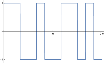
Figure 7: The Bang-Bang control corresponding to the square wave $w_{1}(\omega t)$ as function of time. It self-averages the noise Hamiltonian to zero while preserving the isotropy of the Lindbladian.

By symmetry considerations, ${\mathbfcal H}_{\alpha}=0$ (since $[\tilde{H}_{\alpha}(\omega),H_{\alpha}^{*}(\omega)]\propto[S_{\alpha},S_{\alpha}]=0$). and the depolarizing Lindbldian has renormalized rates:

$${\cal L}\rho=-\frac{\gamma(\omega)}{2}\sum_{j=1}^{3}[\sigma_{j}[\sigma_{j},\rho]],$$

$\gamma(\omega)$ is a more complicated version of Eq. (4.6)

$$\gamma(\omega)=\frac{8}{\pi^{2}}\sum_{n\neq 0}\frac{\tilde{J}(\omega n)}{n^{2}}\sin^{4}\left(\frac{n\pi}{12}\right)p(n)$$ (4.18)

$$p(n)=5+4\cos\left(\frac{n\pi}{6}\right)+2\cos\left(\frac{4n\pi}{3}\right)+(-1)^{n}\left(1+4\cos\left(\frac{n\pi}{2}\right)+2\cos\left(\frac{2n\pi}{3}\right)\right)$$

4.6 Stochastic Harmonic oscillator

The stochastic harmonic oscillator provides a good model for trapped atoms, mechanical oscillators and trapped ions [17]. Since $\mathbbm{1}$ is not a state in an infinite dimensional Hilbert space, the Lindbladian associated with stochastic evolution may have no stationary state.

There are various types of noises one may consider. The first is

$$H_{\xi}=\underbrace{\frac{1}{2}\omega_{c}(p^{2}+x^{2})}_{H_{0}}+\xi_{p}p+\xi_{x}x$$

with $\xi_{x}$ and $\xi_{p}$ Gaussian (possibly correlated) processes. This is known as ‘linear noise’ since it does not affect the frequency of the oscillator.

The interaction Hamiltonian is

$$H_{\xi}^{I}=\xi_{x}\left(x\cos\omega_{c}t+p\sin\omega_{c}t\right)+\xi_{p}\left(p\cos\omega_{c}t-x\sin\omega_{c}t\right)$$

$H_{0}$ is an effective control since $H^{I}_{\xi}$ has vanishing time average. Observe that $ad(x)$ and $ad(p)$ commute since

$$[ad(x),ad(p)]=ad([x,p])=i\,ad(\mathbbm{1})=0$$ (4.19)

It follows from Eq. (1) that the Lindbladian is real (has no Hamiltonian piece) and has the form

$$-2{\cal L}=\Gamma_{x}\,ad(x)ad(x)+\Gamma_{p}\,ad(p)ad(p)+2\Gamma_{xp}\{ad(x),ad(p)\}$$

with matrix $\Gamma\propto\tilde{J}(\omega_{c})$ at the oscillator frequency. Since $ad(x)$ and $ad(p)$ commute, and $spect\big{(}ad(x)\big{)}=spect\big{(}ad(p)\big{)}=(-\infty,\infty)$ and $\Gamma$ is a positive matrix, we have

$$spect({\cal L})=\{-(\eta,\Gamma\eta)|\;\eta\in\mathbb{R}^{2}\}=(-\infty,0]$$

$0$ is in the spectrum but is not associated with an eigenvalue: There is no stationary equilibrium state.

In the case of noise in the frequency of the harmonic oscillator the Hamiltonian is:

$$H_{\xi}=\frac{1}{2}\left((\omega_{c}+2\xi_{p})p^{2}+(\omega_{c}+2\xi_{x})x^{2}\right)=\underbrace{\frac{1}{2}\omega_{c}(p^{2}+x^{2})}_{H_{0}}+\xi_{p}p^{2}+\xi_{x}x^{2}$$

In the interaction picture one has

$$H^{I}_{\xi}=\xi_{p}(p\cos\omega_{c}t-x\sin\omega_{c}t)^{2}+\xi_{x}(x\cos\omega_{c}t+p\sin\omega_{c}t)^{2}$$

Hence

$$\tilde{H}_{\alpha}(0)=[\tilde{H}_{\alpha}(2\omega_{c}),\tilde{H}_{\alpha}(-2\omega_{c})]=\frac{1}{2}(p^{2}+x^{2}),\quad\tilde{H}_{\alpha}(\pm 2\omega_{c})=\frac{1}{4}(-1)^{\alpha}(p\pm ix)^{2}$$

and the Lindbladian is :

$${\cal L}=\underbrace{K_{2}~{}ad~{}\tilde{H}(0)}_{unitary}+\underbrace{\Gamma_{0}\big{(}ad~{}\tilde{H}(0)\big{)}^{2}}_{dephasing}+\underbrace{\Gamma_{2}\left(\big{(}ad~{}\tilde{H}(2\omega_{c})\big{)}^{2}+\big{(}ad~{}\tilde{H}(-2\omega_{c})\big{)}^{2}\right)}_{parametric~{}drive}$$ (4.20)

where $K_{2}\propto\tilde{K}(\omega_{c})$, $\Gamma_{0}\propto\tilde{J}(0)$ and $\Gamma_{2}\propto\tilde{J}(2\omega_{c})$. While all the terms $\left|n\right\rangle\left\langle m\right|$ are eigenstates of the dephasing part with eigenvalues $(m-n)^{2}$ the parametric drive part does not have a steady state and drives the system towards the infinite temperatures.

5 Comparison with stochastic evolutions

Numerical algorithm for solving stochastic evolution equations have two advantages: They can work also beyond weak coupling and evolve states rather than density matrices. They also have several disadvantage: They tend to be slow because of the necessity to accumulating enough statistics; They are prone to long time drifts, and can be adversely affected by a poor random number generator and finally are prone to bugs. Our results on the Lindbland evolutioon can be used to test numerical algorithms for stochastic evolutions in those cases that both apply.

A comparison between Lindbladian evolutions of sections 4.1,4.2,4.3 and stochastic evolutions with Orenstein-Uhlenbeck process is shown in Fig. 8. Three cases have been studied: no control, control by constant $H_{0}$ and Bang-Bang. The weak coupling parameter is $\varepsilon=0.15$ and the agreement is satisfactory. The numerical code is available upon request.

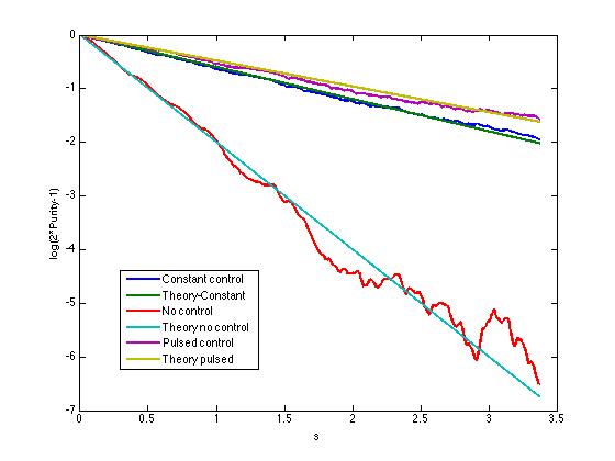
Figure 8: The logarithmic purity of the state, $\log\,Tr(\rho(s)^{2})$ as a function of the coarse grained time $s$, Eq. (1.6) for stochastic evolutions and the corresponding Lindbladians. The weak coupling, Eq. (1.5), is $\varepsilon=0.15$. The numerical grid $\Delta=1$ and correlation time $\tau=20\Delta$. The control parameter is $\omega_{c}\tau=0.5\pi,$ and the stochastic averaging is done on an ensemble of $500$ runs.

6 Summary

We derived the Lindbladian for controlled weakly stochastic evolutions both for small but finite $\varepsilon$ and in the limit $\varepsilon\to 0$ for stationary control. Our results can be used to measure the power spectrum of the noise and to test numerical algorithms for solving stochastic evolution. Several examples are studied in detail.

Appendix A Weak coupling expansion

The purpose of this appendix is to justify the estimate of Eq. (3). This requires a comparison of two different time orderings of the same exponent. Let us first ignore the ordering and consider

$$e^{x}=\sum\frac{x^{n}}{n!},\quad x=-\int_{0}^{t}ds\,{\cal{G}}(s)$$ (A.1)

The Taylor series for the exponent $e^{x}$ is dominated by terms of order $n=O(x)$. In our case this gives $n\sim x\sim H^{2}J\tau t\sim\varepsilon^{2}t/\tau$. Writing the n-th term in the expansion

$$\frac{x^{n}}{n!}=\int_{0\leq s_{1}\leq\dots s_{n}\leq t}\prod_{i=1}^{n}{\cal{G}}(s_{i})\,ds_{i}$$ (A.2)

we conclude that typically $s_{i+1}-s_{i}=O(t/n)=O(\tau/\varepsilon^{2})\gg\tau$.

Figure 9: $(u_{j},v_{j})$ make a dimer. The arc connecting the pair represents the short range interaction in Eq. (A.3). In a typical configuration the distance between dimers is large $O(\tau/\varepsilon^{2})$ and there is at most one dimer in an interval of size $\tau$. The dimer on the left is typical. The dimers on the right lead to the error. The approximation disregards the rare events.

Next let us consider the possible time orderings. The naive $\tilde{T}$ time ordering with respect to the argument of ${\cal{G}}(s)$ implied by Eq. (A.2) differs from the correct $T$-ordering because the relation between ${\cal{G}}$ and ${\cal{H}}$

$${\cal{G}}(s_{i})=-{1\over 2}\int_{u_{i}>v_{i}}du_{i}dv_{i}j(u_{i}-s_{i})j(v_{i}-s_{i})\left({\cal{H}}(u_{i}){\cal{H}}(v_{i})\right)$$ (A.3)

is non -local in time: The ordering of $s_{i}$ does not guarantee the ordering of $(u,v)$. The fact that $j(u-s)$ is fast decaying implies, however, that the nonlocality in time is rather small $\sim\tau$. When $s_{i+1}-s_{i}\gg\tau$ the wrong ordering is almost the same as the correct one.

In order to estimate the error generated by using the $\tilde{T}$ ordering consider more closely the two orderings. Each contribution to the exponent is given as in Eq. (A.2) by some choice of ${0\leq s_{1}\leq\dots s_{n}\leq t}$ and we associate a choice of $u_{i}>v_{i}$ to each $s_{i}$ as in Eq. (A.3). Typically $s_{i+1}-s_{i}\gg\tau\sim|u_{i}-s_{i}|,|v_{i+1}-s_{i+1}|$ and hence $v_{i+1}>u_{i}>v_{i}$ which implies that the two ordering are equivalent. If however there exists some $i$ for which $u_{i}>v_{i+1}$ then the two expressions do not coincide.

Consider for example the case where $u_{j+1}>u_{j}>v_{j+1}>v_{j}$ while all other points are at typical positions. This will lead to an error term of the type

$${\cal{U}}_{n,...j+2}\times\int_{s_{j+1}>s_{j}}ds_{j}ds_{j+1}\int_{u_{j+1}>u_{j}>v_{j+1}>v_{j}}du_{j}du_{j+1}dv_{j}dv_{j+1}{\cal{H}}(u_{j+1})\left[{\cal{H}}(u_{j}),{\cal{H}}(v_{j+1})\right]{\cal{H}}(v_{j})$$ (A.4)

$$\times j(s_{j}-u_{j})j(s_{j}-v_{j})j(s_{j+1}-u_{j+1})j(s_{j+1}-v_{j+1})\times{\cal{U}}_{j-1,...1}$$ (A.5)

Here ${\cal{U}}_{n,...j+2}=\int_{u_{j+1}\leq s_{j+2}\leq\dots s_{n}\leq t}\prod_{i=j+2}^{n}{\cal{G}}(s_{i})\,ds_{i}\;\;{\cal{U}}_{j-1,...1}=\int_{0\leq s_{1}\leq\dots s_{j}\leq v_{j}}\prod_{i=1}^{j-1}{\cal{G}}(s_{i})\,ds_{i}$ correspond to the (unitary) evolution before $t=v_{j}$ and after $t=u_{j+1}$. The integrand in Eq(A.4)is clearly fast decaying whenever its six integration variables are at inter-distance large compared to $\tau$. It thus follows that the main contribution to the integral comes from a region of volume $\tau^{5}t$. The integral is thus at most of order of $\tau^{5}tj^{4}\|{H}\|^{4}\sim\tau^{3}tJ^{2}\|{H}\|^{4}=\varepsilon^{4}t/\tau$. Other nontypical cases (e.g. $u_{j}>u_{j+1}>v_{j+1}>v_{j}$) lead to error terms of a similar general form which again scale as $\varepsilon^{4}t/\tau$.

The error terms we found are of the form $\int_{0}^{t}ds\,{\cal{U}}(s,t)\Delta{\cal{G}}(s){\cal{U}}(0,s)$ for some $\Delta{\cal{G}}$ which is quartic in ${\cal{H}}$. This suggests defining an improved generator as ${\cal{G}}\mapsto{\cal{G}}+\Delta{\cal{G}}$. We however did not pursue this direction here.

Appendix B The spectrum of the super-operators of angular momenta

The adjoint representation $ad(S)$ of a representation $S$ is constructed as the tensor product of $S$ with its dual (contragredient) representation $S^{*}$. Since $SU(2)$ has a single representaions in each dimension, it is obvious that $S^{*}\simeq S$. It thus follows that

$$ad(S)=S\otimes S^{*}=S\otimes S=0\oplus 1\oplus 2\oplus......\oplus(2S)$$

The spectrum (including multiplicities) of various operators such as $ad(S_{z})$ and $\sum ad(S_{j})ad(S_{j})$ is then easily deduced

$$Spect\big{(}ad(S_{z})\big{)}=\bigcup_{j=0,\dots 2S}\{m|m=-j,\dots j\}$$

$$Spect\left(\sum_{i=x,y,z}\big{(}ad(S_{i})^{2}\big{)}\right)=\bigcup_{j=0,\dots 2S}\{j(j+1)|m=-j,\dots j\}$$

$$Spect\left(\sum_{i=x,y}\big{(}ad(S_{i})^{2}\big{)}\right)=\bigcup_{j=0,\dots 2S}\{j(j+1)-m^{2}|m=-j,\dots j\}$$

In particular the eigenvalue zero appears in $Spect\big{(}ad(S_{x})^{2}+ad(S_{y})^{2}\big{)}$ with trivial multilicity 1. This last fact could also be deduced from Schur’s lemma since by positivity $\big{(}ad(S_{x})^{2}+ad(S_{y})^{2}\big{)}\rho=0$ imply $ad(S_{x})\rho=ad(S_{y})\rho=0$ and hence also $ad(S_{z})\rho=-i[ad(S_{x}),ad(S_{r})]\rho=0$.

Appendix C Effective control

In dynamical decoupling one is interested in making ${\cal L}$ small at the price of strong control, $\omega_{c}\tau\gg 1$. Since $\tilde{J}(\omega)$ is small for large argument and since the terms $\omega\neq 0$ in Eq. (1) tend to be of order $\tilde{J}(\omega_{c})$ the “bad term” in ${\cal L}$ is the one with $\omega=0$. We say that the control is “effective” if $\tilde{H}_{\alpha}(\omega=0)=0$. The notion is independent of $J_{\alpha}(u)$, which is often not known.

Consider first strong continuous controls. Let $P_{j}(t)$ be the (instantaneous) spectral projections of $H_{c}$:

$$H_{c}(t)=\omega_{c}\sum e_{j}(t)P_{j}(t)$$

and suppose that $P_{j}(t)$ vary smoothly with $t$ and that the $e_{j}(t)$ do not cross. Then, by the adiabatic theorem, for $\omega_{c}$ large

$$H_{\alpha}^{I}(t)\approx\sum_{j,k}e^{i\omega_{c}\int_{0}^{t}(e_{j}(u)-e_{k}(u))du}P_{j}(t)H_{\alpha}P_{k}(t)\underset{\omega_{c}\to\infty}{\longrightarrow}\sum_{j}P_{j}(t)H_{\alpha}P_{j}(t)$$

(in the sense of distributions.) It follows that the control is effective if, for all $t$,

$$\sum_{j}P_{j}(t)H_{\alpha}P_{j}(t)=0$$ (C.1)

Bang-Bang at times $t_{j}$ is effective if $\tilde{H}_{\alpha}(\omega=0)=0$, which is the case if $H_{I}(t)$ has zero average, i.e.

$$\forall\alpha,\;\;\sum_{j}(t_{j+1}-t_{j})V(t_{j})H_{\alpha}V(t_{j})=0$$

References

- [1] Robert Alicki and Mark Fannes. Quantum dynamical systems. status: published, 2001.
- [2] Robert Alicki, Daniel A Lidar, and Paolo Zanardi. Internal consistency of fault-tolerant quantum error correction in light of rigorous derivations of the quantum markovian limit. Physical Review A, 73(5):052311, 2006.
- [3] Ido Almog, Yoav Sagi, Goren Gordon, Guy Bensky, Gershon Kurizki, and Nir Davidson. Direct measurement of the system-environment coupling as a tool for understanding decoherence and dynamical decoupling. J. Phys. B, 44:154006, 2011.
- [4] Heinz-Peter Breuer and Francesco Petruccione. The Theory of Open Quantum Systems. Oxford University Press, USA, 2007.
- [5] E Brian Davies. Markovian master equations. Communications in mathematical Physics, 39(2):91–110, 1974.
- [6] Edward Brian Davies. Quantum theory of open systems. 1976.
- [7] Berthold-Georg Englert and Giovanna Morigi. Five lectures on dissipative master equations. In Andreas Buchleitner and Klaus Hornberger, editors, Coherent Evolution in Noisy Environments, volume 611 of Lecture Notes in Physics, pages 55–106. Springer Berlin Heidelberg, 2002.
- [8] M. Fraas. Adiabatic theorem for a class of quantum stochastic equations. ArXiv e-prints, July 2014.
- [9] Goren Gordon, Gershon Kurizki, and Daniel A Lidar. Optimal dynamical decoherence control of a qubit. arXiv preprint arXiv:0804.2691, 2008.
- [10] V. Gorini, A. Kossakowski, and E.C.G. Sudarshan. Completely positive dynamical semigroups of -level systems. J. Math. Phys., 17(5):821–825, 1976.
- [11] Daniel F. V. James and Jonathan Jerkel. Effective hamiltonian theory and its applications in quantum information. Canadian Journal of Physics, 85:625–632, 2007.
- [12] A. G. Kofman and G. Kurizki. Unified theory of dynamically suppressed qubit decoherence in thermal baths. Phys. Rev. Lett., 93:130406, Sep 2004.
- [13] G. Lindblad. On the generators of quantum dynamical semigroups. Comm. Math. Phys., 48:119–130, 1976.
- [14] Carlos Meriles, Liang Jiang, Garry Goldstein, Jonathan Hodges, Jeronimo Maze, Mikhail Lukin, and Paola Cappellaro. Imaging mesoscopic nuclear spin noise with a diamond magnetometer. THE JOURNAL OF CHEMICAL PHYSICS, 133:124105, 2010.
- [15] Y Romach, C Müller, T Unden, L. J. Rogers, T Isoda, K.M. Itoh, M. A. Markham, Stacey, J Meijer, S Pezzagna, B Naydenov, L.P. McGuinness, N. Bar-Gill, and F Jelezko. Nuclear magnetic resonance spectroscopy on a (5-nanometer)3 sample volume. Arxiv, 1404:3879, 2014.
- [16] D. Salgado and J. L. Sanchez-Gomez. Lindbladian Evolution with Selfadjoint Lindblad Operators as Averaged Random Unitary Evolution. eprint arXiv:quant-ph/0208175, August 2002.
- [17] S. Schneider and G. J. Milburn. Decoherence and fidelity in ion traps with fluctuating trap parameters. Phys. Rev. A., 59:3766, 1999.
- [18] Herbert Spohn and Joel L. Lebowitz. Irreversible thermodynamics for quantum systems weakly coupled to thermal reservoirs. Advances in Chemical Physics, pages 109–142, 1978.
- [19] T Staudacher, F Shi, S Pezzagna, J Meijer, J Du, C Meriles, F Reinhard, and J Wrachtrup. Nuclear magnetic resonance spectroscopy on a (5-nanometer)3 sample volume. Science, 399(6119):561, 2013.
- [20] K. Szczygielski. On the application of Floquet theorem in development of time-dependent Lindbladians. ArXiv e-prints, March 2014.