Universal Statistical Properties of Inertial-particle Trajectories in Three-dimensional, Homogeneous, Isotropic, Fluid Turbulence

Abstract

We uncover universal statistical properties of the trajectories of heavy inertial particles in three-dimensional, statistically steady, homogeneous, and isotropic turbulent flows by extensive direct numerical simulations. We show that the probability distribution functions (PDFs) $P(\phi)$, of the angle $\phi$ between the Eulerian velocity ${\bf u}$ and the particle velocity ${\bf v}$, at this point and time, shows a power-law region in which $P(\phi)\sim\phi^{-\gamma}$, with a new universal exponent $\gamma\simeq 4$. Furthermore, the PDFs of the trajectory curvature $\kappa$ and modulus $\theta$ of the torsion $\vartheta$ have power-law tails that scale, respectively, as $P(\kappa)\sim\kappa^{-h_{\kappa}}$, as $\kappa\to\infty$, and $P(\theta)\sim\theta^{-h_{\theta}}$, as $\theta\to\infty$, with exponents $h_{\kappa}\simeq 2.5$ and $h_{\theta}\simeq 3$ that are universal to the extent that they do not depend on the Stokes number ${\rm St}$ (given our error bars). We also show that $\gamma$, $h_{\kappa}$ and $h_{\theta}$ can be obtained by using simple stochastic models. We characterize the complexity of heavy-particle trajectories by the number $N_{\rm I}(t,{\rm St})$ of points (up until time $t$) at which $\vartheta$ changes sign. We show that $n_{\rm I}({\rm St})\equiv\lim_{t\to\infty}\frac{N_{\rm I}(t,{\rm St})}{t}\sim{\rm St}^{-\Delta}$, with $\Delta\simeq 0.4$ a universal exponent.

Inertial particles, advected by turbulent fluid flows, show rich dynamics that are of great interest, not only because of potential applications in geophysical Csa73 , atmospheric sha03 ; gra+wan13 ; fal+fou+ste02 , astrophysical Arm10 , and industrial processes eat+fes94 ; pos+abr02 , but also because they pose challenging questions of fundamental importance in the fluid dynamics and nonequilibrium statistical mechanics of such flows. Experimental, theoretical, and especially numerical investigations, which have been carried out over the past few decades, have shown that neutrally buoyant tracers (or Lagrangian particles) respond very differently to turbulent flows than do heavy, inertial particles toschirev ; becoverview ; for instance, tracers get distributed uniformly in space in a turbulent, incompressible flow, but, in the same flow, heavy, inertial particles cluster TOSCHI ; Biferale , especially when the Stokes number ${\rm St}\simeq 1$, where ${\rm St}=\tau_{s}/\tau_{\eta}$, with $\tau_{s}$ the particle-response or Stokes time and $\tau_{\eta}$ the Kolmogorov time, at the dissipation length scale $\eta$. We study the statistical properties of the geometries of heavy-inertial-particle trajectories; such inertial-particle-trajectory statistics have not received much attention hitherto in homogeneous, isotropic, three-dimensional (3D) fluid turbulence.

Our direct-numerical-simulation (DNS) studies of these statistical properties yield new and universal scaling exponents that characterize heavy-particle trajectories. We calculate the probability distribution functions (PDFs) of the angle $\phi$ between the Eulerian velocity ${\bf u}({\bf x},t)$, at the point ${\bf x}$ and time $t$, and the velocity ${\bf v}$ of an inertial particle at this point and time, PDFs of the curvature $\kappa$ and torsion $\vartheta$ of inertial-particle trajectories, and several joint PDFs. In particular, we find that the PDF $P(\phi)$ shows a power-law region in which $P(\phi)\sim\phi^{-\gamma}$, with an exponent $\gamma\simeq 4$, which has never been considered so far; the extent of this power-law regime decreases as ${\rm St}$ increases; we find good power-law fits if $0<{\rm St}\lesssim 0.7$; in this range $\gamma$ is universal, in as much as it does not depend on ${\rm St}$ and the fluid Reynolds number ${\rm Re}$ (given our error bars). The PDFs of $\kappa$ and $\theta=|\vartheta|$ show power-law tails for large $\kappa$ and $\theta$, respectively, with power-law exponents $h_{\kappa}$ and $h_{\theta}$ that are also universal. We calculate the number of points, per unit time, at which the torsion $\vartheta$ changes sign along a particle trajectory; this number $n_{I}({\rm St})\sim{\rm St}^{-\Delta}$, as ${\rm St}\to 0$, with $\Delta\simeq 0.4$ another universal exponent. We show how simple stochastic models can be used to obtain the exponents $\gamma$, $h_{\kappa}$, and $h_{\theta}$; however, the evaluation of $\Delta$ requires the velocity field from the Navier-Stokes equation.

Table 1: Parameters for our runs ${\bf R1}$ and ${\bf R2}$ with $N^{3}$ collection points, $\nu$ the coefficient of kinematic viscosity, $\delta t$ the time step, $N_{p}$ the number of particles, $k_{max}$ the largest wave number in the simulation, $\eta$ and $\tau_{\eta}$ the dissipation length and time scales, respectively, $\lambda$ the Taylor microscale, $Re_{\lambda}$ the Taylor-microscale Reynolds number, $I_{l}$ the integral length scale, and $T_{eddy}$ the large-eddy turnover time.

Run	$N$	$\nu$	$\delta t$	$N_{p}$	$Re_{\lambda}$	$k_{max}\eta$	$\epsilon$	$\eta$	$\lambda$	$I_{l}$	$\tau_{\eta}$	$T_{eddy}$
R1	$256$	$3.8\times 10^{-3}$	$5\times 10^{-4}$	$40,000$	$43$	$1.56$	$0.49$	$1.82\times 10^{-2}$	$0.16$	$0.51$	$8.76\times 10^{-2}$	$0.49$
R2	$512$	$1.2\times 10^{-3}$	$2\times 10^{-4}$	$100,000$	$79$	$1.21$	$0.69$	$7.1\times 10^{-3}$	$0.08$	$0.47$	$4.18\times 10^{-2}$	$0.41$

We perform a DNS spectral of the incompressible, three-dimensional (3D), forced, Navier-Stokes equation

$$\partial_{t}{\bf u}+({\bf u}\cdot\nabla){\bf u} = \nu\nabla^{2}{\bf u}-\nabla p+{\bf f},$$ (1)

$$\nabla\cdot{\bf u} = 0,$$ (2)

where ${\bf u}$, $p$, ${\bf f}$, and $\nu$ are the velocity, pressure, external force, and the kinematic viscosity, respectively. Our simulation domain is a cubical box with sides of length $2\pi$ and periodic boundary conditions in all three directions. We use $N^{3}$ collocation points, a pseudospectral method with a $2/3$ dealiasing rule spectral , a force that yields a constant energy injection (see, e.g., Refs. Lamorgese ; Ganapati ), with an energy-injection rate $P$, and a second-order Adams-Bashforth method for time marching Ganapati . In several experiments (a) the radius of the particle $\mathit{a}\ll\eta$, with $\eta$ the Kolmogorov dissipation scale of the advecting fluid (i.e., the particle-scale Reynolds number is very small), (b) particle interactions are negligible, (e.g., if the number density of particles is low), (c) the particle density $\rho_{p}\gg\rho_{f}$, the fluid density, (d) typical particle accelerations exceed considerably the acceleration because of gravity, and (e) the particles do not affect the fluid velocity; if these conditions hold, then the position ${\mathbf{x}}(t)$ and velocity ${\bf v}(t)$, at time $t$, of a small, rigid, particle (henceforth, a heavy, inertial particle), in an incompressible flow, evolve as follows maxey83 ; gatignol83 ; bec2006acceleration :

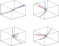
Figure 1: (Color online) (a) Plots of the unit vectors along the directions of the particle and fluid velocities (in blue and red, respectively) at the position of the particle, and the trajectory of the particle in the neighbourhood of the particle position (black dots), at four different time instants for ${\rm St}=1.0$. (b) Cumulative PDFs of the angle $\phi$ between $\mathbf{u}$ and $\mathbf{v}$ ($Q(\alpha)\equiv P(\phi\geq\alpha)$), for ${\rm St}=0.2$ (blue circles), ${\rm St}=0.5$ (green triangles), ${\rm St}=0.7$ (brown squares), ${\rm St}=1.0$ (red pluses), and ${\rm St}=1.4$ (purple stars), obtained by using the rank-order method  dmitra ; the slope of the black dashed line is $-3$; the inset shows plots of PDF $P(\phi)$, (c) coefficient of correlation $R$ between $u_{x}$ and $v_{x}$ as a function of ${\rm St}$ (red circles) obtained from DNS data, black line shows the exponential fit.

$$\frac{d}{dt}{\bf v}(t) = -\frac{{\bf v}(t)-{\bf u}({\bf x},t)}{\tau_{s}};$$ (3)

and

$$\frac{d}{dt}{\mathbf{x}}(t) = {\bf v}(t);$$ (4)

here ${\bf u}({\bf x},t)$ denotes the Eulerian velocity field at position ${\bf x}$ and $\tau_{s}=(2\mathit{a}^{2})/(9\nu\rho_{\rm f})$. To obtain the statistical properties of the particle paths, we follow the trajectories of $N_{p}$ particles in our simulation, use trilinear interpolation num_rec to calculate the components of the velocity and the velocity-gradient tensor at the positions of the particles. Table 1 lists the parameters we use. We solve for the trajectories of $N_{p}$ inertial particles, for each of which we solve Eqs.(3) and (4) with an Euler scheme, which is adequate because, in time $\delta t$, a particle crosses at most one-tenth of the grid spacing.

At the position of a particle, the particle and fluid velocities are different because of the Stokes drag. We expect this difference to increase with ${\rm St}$. In Fig. 1 (a) we show plots of the unit vectors, along the directions of the particle and fluid velocities (in red and green, respectively), at the position of the particle, and the trajectory of the particle in the neighborhood of the particle position (blue dots), at four different time instants (for a video see Ref. supp ). To quantify the statistics of the angle between these unit vectors, we show in the inset of Fig. 1 (b) plots of the PDFs $P(\phi)$ of the angle $\phi$ between $\mathbf{\hat{v}}$ and $\mathbf{\hat{u}}$, for different values of ${\rm St}$. For small ${\rm St}$, $P(\phi)$ shows a peak near $\phi\simeq 0$; this peak broadens when we increase ${\rm St}$. Log-log plots of the cumulative PDFs $Q(\phi)$ [Fig. 1 (b)] reveal that, especially for small values of ${\rm St}$, there is a remarkable and distinct power-law regime in which $Q(\phi)\sim\phi^{-\gamma+1}$, with a scaling exponent $\gamma\simeq 4$, i.e., the PDF $P(\phi)\sim\phi^{-4}$. Although $\gamma$ is insensitive to the value of ${\rm St}$ (given our error bars), the extent of the scaling regime decreases as we increase ${\rm St}$.

A particle trajectory is a 3D curve that we characterize by its tangent ${\mathbf{t}}$, normal ${\mathbf{n}}$, and binormal ${\mathbf{b}}$, which are diff_geom ; diff_geom2 ; wbraun

$${\mathbf{t}}=\frac{d{\mathbf{r}}}{ds};\;{\mathbf{n}}=\frac{1}{\kappa}\frac{d{\mathbf{t}}}{ds};\;{\mathbf{b}}={\mathbf{t}}\times{\mathbf{n}};$$ (5)

these evolve according to the Frenet-Serret formulas as:

$$\frac{d{\mathbf{t}}}{ds}=\kappa{\mathbf{n}};\;\frac{d{\mathbf{n}}}{ds}=\vartheta{\mathbf{b}}-\kappa{\mathbf{t}};\;\frac{d{\mathbf{b}}}{ds}=-\vartheta{\mathbf{n};}$$ (6)

here ${\mathbf{r}}$ and $s$ indicate the particle position and arc length along the particle trajectory, respectively. The curvature $\kappa$ and the torsion $\vartheta$ of a particle trajectory are (dots indicate time derivatives)

$$\kappa=\frac{|{\bf v}\times{\bf\dot{v}}|}{|{\bf v}|^{3}}=a_{n}/v^{2};\;\vartheta=\frac{{\bf v}\cdot({\bf\dot{v}}\times{\bf\ddot{v}})}{({\bf v}\cdot{\bf v})^{3}\kappa^{2}}.$$ (7)

Here $a_{n}$ is the normal component of the acceleration $\mathbf{a}$, $v=|\bf v|$, and $\theta=|\vartheta|$. From Eqs.(3) and (6) it follows that ${\mathbf{u}}$, ${\mathbf{v}}$, and ${\mathbf{a}}$ can be expressed as ${\mathbf{u}}=u\cos{\phi}{\mathbf{t}}+u\sin{\phi}{\mathbf{n}}$, ${\mathbf{v}}=v{\mathbf{t}}$, and ${\mathbf{a}}=a_{t}{\mathbf{t}}+a_{n}{\mathbf{n}}$, whence we obtain

$$\sin{\phi}=\frac{a_{n}\tau_{s}}{u}=\frac{\kappa v^{2}\tau_{s}}{u}.$$ (8)

We find, in agreement with Ref. bec2006acceleration , that the PDFs of the normal component $a_{n}$ the tangential component $a_{t}$ and $a=|\mathbf{a}|$ exhibit tails supp , which can be fit to exponential forms with decay rates $\alpha_{n}$, $\alpha_{t}$, and $\alpha$, respectively; these decay rates decrease as ${\rm St}$ increases (Table  3). By contrast, the PDFs $P(\kappa)$ and $P(\theta)$ have power-law tails that scale as $P(\kappa)\sim\kappa^{-h_{\kappa}}$, as $\kappa\to\infty$, and $P(\theta)\sim\theta^{-h_{\theta}}$, as $\theta\to\infty$, with exponents $h_{\kappa}\simeq 2.5$ and $h_{\theta}\simeq 3$ that do not depend on ${\rm St}$ (given our error bars) . We obtain these exponents accurately from the cumulative PDFs $Q_{\kappa}(\kappa\eta)$ and $Q_{\tau}(\theta\eta)$, which we obtain by using a rank-order method dmitra to overcome binning errors and which we show in the log-log plots of Figs. 2 (a) and (b), respectively, for representative values of ${\rm St}$. The slopes of the straight-line parts (blue lines) in these plots yield $h_{\kappa}+1$ and $h_{\theta}+1$; we list $h_{\kappa}$ and $h_{\theta}$ in Table 3; to obtain the error bars on these exponents we carry out a local-slope analysis Perlekar for the power-law regimes in these cumulative PDFs (see the insets of Figs. 2 (a) and (b)).

We use the torsion $\vartheta$ to characterize the complexity of a particle track by computing the number, $N_{I}(t,{\rm St})$, of points at which $\vartheta$ changes sign up until time $t$. We propose that, for a given value of ${\rm St}$,

$$n_{I}({\rm St})\equiv\lim_{t\to\infty}\frac{N_{I}(t,{\rm St})}{t}$$ (9)

exists and is a natural measure of its complexity. In Fig. 2 (c), we plot $N_{I}/(t/T_{eddy})$ versus the dimensionless time $t/T_{eddy}$, for two representative values of ${\rm St}$. From such plots we obtain $n_{I}({\rm St})$ (see Eq. (9)), which we depict as a function of ${\rm St}$ in the inset of Fig. 2 (c), and whence we find

$$n_{I}({\rm St})\sim{\rm St}^{-\Delta},$$ (10)

where $\Delta\simeq 0.4$. This indicates that, as ${\rm St}\to 0$, particle trajectories become more and more contorted in all three spatial dimensions (cf. Ref. geometry2d for the analog of this result for 2D fluid turbulence).

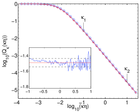
Figure 2: (Color online) Cumulative PDFs of, (a) the curvature $\kappa$ and (b) the magnitude of the torsion $\theta$ of the trajectories of heavy inertial particles, for $St=0.2$ (in blue) and $1.0$ (in red), obtained using rank order method. Inset: the values of the local slope of the tail, for $St=1.0$. (c) Number of inflection points per unit time (see Eq. (7)) as a function of dimensionless time $t/T_{eddy}$, for $St=0.2$, (red curve), and $St=1.4$, (blue curve); the inset shows the plot of the number of inflection points per unit time $n_{I}$, as a function of ${\rm St}$, obtained from run R2

The analogs of the exponents $h_{\kappa}$ and $h_{\theta}$ have been obtained in studies with Lagrangian tracers in DNSs wbraun ; scagliarini and experiments curvatureprl . The exponents obtained in both these studies, for tracers, are within error bars of those that we obtain here for heavy inertial particles (see Table 3). In Refs. scagliarini ; curvatureprl it has been suggested that the value of $h_{\kappa}$ can be obtained by noting that large values of $\kappa$ are associated with small values of $v$; furthermore, $h_{\kappa}=2.5$ can be obtained analytically by assuming that the joint PDF $\mathcal{P}(a_{n},v)$ factors into the products of the PDFs $P(a_{n})$ and $P(v)$. A similar argument scagliarini yields $h_{\theta}=3$. These arguments can be extended to the case of heavy inertial particles and used, therefore, to understand the proximity of the values of $h_{\kappa}$ and $h_{\theta}$ (see Table 3) to those for Lagrangian tracers. In Fig. 5, we plot joint PDFs of $\kappa$ and $v$, and $\kappa$ and $a_{n}$ for two representative values of ${\rm St}$ (${\rm St}=0.2$ left column, ${\rm St}=1.4$ right column). Clearly, large values of $\kappa$ are correlated with small values of $v$ but not with large values of $a_{n}$; i.e., high-curvature parts of particle trajectories are associated with regimes of a track where the particle velocity reverses. Furthermore, we show in  supp that the assumption $\mathcal{P}(a_{n},v)\equiv P_{an}(a_{n})P_{v}(v)$ made in  scagliarini does not hold very well.

To understand the universal power laws mentioned above, we use a simple stochastic model for the Eulerian velocity field supp , and integrate Eqs.(3) and (4) to find particle trajectories. We find that such a simple model, in which the Eulerian velocity field is given by Eqs.(4)-(6) in supp , reproduces the exponents $\gamma$, $h_{\kappa}$, and $h_{\theta}$ accurately supp but not $\Delta$.

We also show numerically that, if we consider the components of fluid and particle velocities $u_{i}$ and $v_{j}$, where $i,j\in(x,y,z)$, to be correlated Gaussian random variates with mean zero, such that the coefficient of correlation between them $\rho(u_{i},v_{j})\equiv\langle u_{i}v_{j}\rangle/\sqrt{\langle u_{i}^{2}\rangle\langle v_{j}^{2}\rangle}$ is a function of ${\rm St}$, such that, $\rho(u_{i},v_{j})=R({\rm St})\delta_{ij}$, then we get the same values of the exponents, $\gamma$, $h_{\kappa}$, and $h_{\theta}$  supp as in Table 3. The plot of $\log_{10}(R)$ versus ${\rm St}$ in Fig. 1 (c), shows that $R$ decays exponentially with increasing ${\rm St}$ in our DNS of Eqs. (1)-(3).

We hope that our results will stimulate new experimental studies ewsaw of the geometries of inertial-particle trajectories in turbulent flows. Our results for $P(\phi)$, $P(\kappa)$, $P(\theta)$, and $n_{I}({\rm St})$ can be used to constrain models for the statistical properties of inertial particles in turbulent flows model1 ; model2 . In particular, we show that simple stochastic models can yield $\gamma$, $h_{\kappa}$, and $h_{\theta}$ but not the exponent $\Delta$ Ref. supp .

The exponent $\Delta$ has not been introduced in 3D fluid turbulence so far. Our results imply that $n_{\rm I}({\rm St})$ has a power-law divergence, as ${\rm St}\to 0$. This is suppressed eventually, in any finite-resolution DNS, which can only achieve a finite value of $Re_{\lambda}$. This is the analog of the finite-size suppression of divergences, in thermodynamic functions, at an equilibrium critical point fssprivman . Furthermore, the limit ${\rm St}\to 0$ is singular, so it is not clear a priori that it should yield the same results, for the properties we study, as those in the Lagrangian case ${\rm St}=0$.

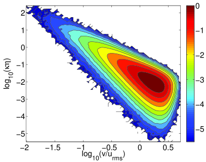
Figure 3: (Color online) Filled contour plots of the joint PDFs of the curvature and velocity of the particle (top row) and curvature and normal component of the particle acceleration (bottom row).

Table 2: Decay constants $\alpha$, $\alpha_{t}$ and $\alpha_{n}$, from the exponential fit to the PDFs of the acceleration, tangential component of acceleration and normal component of the acceleration, respectively, and the exponents $h_{\kappa}$ and $h_{\theta}$ from the power-law fits to the tails of the cumulative PDFs of the curvature $\kappa$ and torsion $\theta$, respectively, for the different values of ${\rm St}$.

${\rm St}$	$\alpha$	$\alpha_{t}$	$\alpha_{n}$	$h_{\kappa}$	$h_{\theta}$
$0.2$	$0.31\pm 0.08$	$0.19\pm 0.09$	$0.30\pm 0.07$	$2.4\pm 0.2$	$3.0\pm 0.3$
$0.5$	$0.21\pm 0.08$	$0.13\pm 0.08$	$0.20\pm 0.09$	$2.6\pm 0.3$	$3.1\pm 0.3$
$0.7$	$0.18\pm 0.06$	$0.11\pm 0.09$	$0.17\pm 0.08$	$2.5\pm 0.2$	$3.0\pm 0.2$
$1.0$	$0.15\pm 0.04$	$0.10\pm 0.07$	$0.14\pm 0.06$	$2.48\pm 0.09$	$2.9\pm 0.2$
$1.4$	$0.13\pm 0.05$	$0.08\pm 0.06$	$0.11\pm 0.06$	$2.4\pm 0.1$	$3.1\pm 0.2$

We thank J. Bec, A. Brandenburg, B. Mehlig, E.W. Saw, and D. Vincenzi for discussions, and particularly A. Niemi, whose study of the intrinsic geometrical properties of polymers poly11 inspired our work on particle trajectories, and S. S. Ray for an introduction to the first of the stochastic models we use in Ref supp . This work has been supported in part by the European Research Council under the AstroDyn Research Project No. 227952 (DM), Swedish Research Council under grant 2011-542 (DM), NORDITA visiting PhD students program (AG), and CSIR, UGC, and DST (India) (AB, AG and RP). We thank SERC (IISc) for providing computational resources. AG, PP, and RP thank NORDITA for hospitality under their Particles in Turbulence program; DM thanks the Indian Institute of Science for hospitality.

Supplemental Material

This Supplemental Material contains some probability distribution functions (PDFs) and joint PDFs that augment the figures given in the main part of this paper. We give semilogarithmic plots of the PDFs $P_{\mathrm{a}}$, $P_{\mathrm{at}}$, and $P_{\mathrm{an}}$ of the acceleration (Fig. 4 (a)), its tangential component (Fig. 4 (b)), and its normal component (Fig. 4 (c)), respectively. The right tails of these PDFs can be fit to exponential forms; in particular,

$$P_{\mathrm{a}}(a/(u_{rms}/\tau_{\eta})) \sim \exp\left(-\frac{a/(u_{rms}/\tau_{\eta})}{\alpha}\right),$$ (11)

$$P_{\mathrm{at}}(a_{t}/(u_{rms}/\tau_{\eta})) \sim \exp\left(-\frac{a_{t}/(u_{rms}/\tau_{\eta})}{\alpha_{t}}\right),$$ (12)

$$P_{\mathrm{an}}(a_{n}/(u_{rms}/\tau_{\eta})) \sim \exp\left(-\frac{a_{n}/(u_{rms}/\tau_{\eta})}{\alpha_{n}}\right),$$ (13)

with decay rates $\alpha$, $\alpha_{t}$, and $\alpha_{n}$ whose values we list, for different values of the Stokes number ${\rm St}$, in TABLE  3. All these decay rates decrease as ${\rm St}$ increases.

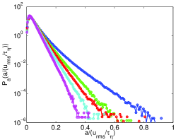
Figure 4: (Color online) Probability distribution functions PDFs of (a) the modulus of the particle acceleration, (b) the tangential component of the particle acceleration, and (c) the normal component of the particle acceleration, for ${\rm St}=0.2$ (blue curve), ${\rm St}=0.5$ (green curve), ${\rm St}=0.7$ (red curve), ${\rm St}=1.0$ (cyan curve), ${\rm St}=1.4$ (magenta curve), from run R2.

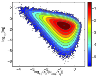
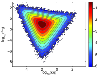
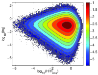
Figure 5: (Color online) Joint PDFs of (a) the torsion and the normal component of the acceleration, (b) the torsion and curvature of the particle track, and (c) the torsion of the particle track and the helicity of the flow at the position of the particle, for four different values of ${\rm St}$.

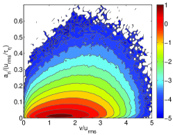
Figure 6: (Color online) Contours of the joint PDFs $\mathcal{P}(a_{n},v)$ (left column), the product of the independent PDFs $P_{an}(a_{n})P_{v}(v)$ (middle column), and $\log_{10}(\mathcal{P}(a_{n},v)/(P_{an}(a_{n})P_{v}(v)))$ (right column).

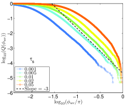
Figure 7: (Color online) Analogs of (a) Fig.1(b), (b) Fig.2(a), and (c) Fig.2(b), of the main paper, obtained by using the stochastic model described above (Eqs. (4)-(7)).

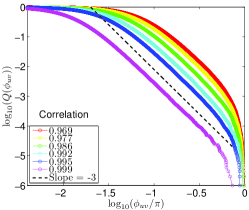
Figure 8: (Color online) Analogs of (a) Fig.1(b), (b) Fig.2(a), and (c) Fig.2(b), of the main paper, obtained by using the simple models of Eqs. (8)-(9).

Table 3: Decay constants $\alpha$, $\alpha_{t}$ and $\alpha_{n}$ (Eqs. 13), for different values of ${\rm St}$.

${\rm St}$	$\alpha$	$\alpha_{t}$	$\alpha_{n}$
$0.2$	$0.31\pm 0.08$	$0.19\pm 0.09$	$0.30\pm 0.07$
$0.5$	$0.21\pm 0.08$	$0.13\pm 0.08$	$0.20\pm 0.09$
$0.7$	$0.18\pm 0.06$	$0.11\pm 0.09$	$0.17\pm 0.08$
$1.0$	$0.15\pm 0.04$	$0.10\pm 0.07$	$0.14\pm 0.06$
$1.4$	$0.13\pm 0.05$	$0.08\pm 0.06$	$0.11\pm 0.06$

Row (a) of Fig. 5 shows joint PDFs of $\theta$ and $a_{n}$; these joint PDFs demonstrate that large values of the magnitude of the torsion $\theta$ are associated with small values of $a_{n}$. Row (b) of Fig. 5 depicts joint PDFs of $\kappa$ and $\theta$. Row (c) of Fig. 5 shows joint PDFs of $\theta$ and the helicity $H$ of the flow at the position of the particle. These joint PDFs do not depend strongly on ${\rm St}$ and they demonstrate that small and the large values of $\theta$ are associated predominantly with $H\simeq H_{rms}$, where the subscript $rms$ denotes root-mean-square value.

To test the assumption that $\mathcal{P}(a_{n},v)\equiv P_{\mathrm{an}}(a_{n})P_{v}(v)$,  scagliarini we plot the joint PDFs of $a_{n}$ and $v$ and the product $P_{\mathrm{an}}(a_{n})P_{v}(v)$ side by side, for different values of ${\rm St}$ in Fig. 6. These joint PDFs show that the statistical-independence assumption $\mathcal{P}(a_{n},v)\equiv P_{\mathrm{an}}(a_{n})P_{v}(v)$, made in  geometry3d, does not hold very well.

We also use the following stochastic model for the velocity field ${\bf u}$, to obtain all the statistical properties of particle trajectories that we have discussed in the main part of this paper. We first define

$$C_{ij}^{\pm} = \cos(i\pm j),$$ (14)

$$S_{ij}^{\pm} = \sin(i\pm j),$$ (15)

where $i,j\in(x,y,z)$, are the Cartesian co-ordinates. Then we take all three components of the velocity field $(u_{x},u_{y},u_{z})$ as linear combinations of $C_{ij}^{\pm}$ and $S_{ij}^{\pm}$, with coefficients $\zeta_{i}$, which evolve in time according to the following stochastic equation:

$$\zeta_{i}(t+\delta t) = \zeta_{i}(t)\exp(-\delta t/T_{cor})$$ (16)

$$+ \xi_{i}(t)\sqrt{\frac{1-\exp(-2\delta t/T_{cor})}{2}},$$ (17)

where $T_{cor}$ is the correlation time and $\xi_{i}(t)$ are chosen from a normal distribution samriddhi ; becoverview . By using the above model we integrate Eqs.(3) and (4) in the main paper, to obtain particle trajectories. Figures 7 (a), (b), and (c) shows the PDFs of the angle $\phi$, curvature $\kappa$, and torsion $\theta$, respectively, for the model. We find that the PDFs $P(\phi)$, $P(\kappa)$ and $P(\theta)$, obtained from the stochastic model described above, yield the same values for the exponents $\gamma$, $h_{\kappa}$ and $h_{\theta}$ as we obtain from our full DNS in the main paper. However this model does not yield the form of $n_{I}({\rm St})$ (given in Fig. 2 (c) in the main paper) and, therefore, this model does not yield the exponent $\Delta$.

Consider now another simple model in which components of the particle and fluid velocities are correlated, random Gaussian variates, with

$$\langle u_{i}\rangle=\langle v_{i}\rangle=0;\\ \sigma_{u_{i}}=\sigma_{v_{i}}=1;\\$$ (18)

here $i=(x,y,z)$, $\langle.\rangle$ represents the average, and $\sigma_{u_{i}}$ and $\sigma_{v_{i}}$ are the standard deviations of $u_{i}$ and $v_{i}$, respectively. We consider the coefficient of correlation $\rho(u_{i},v_{j})$ as a function of ${\rm St}$, namely,

$$\rho(u_{i},v_{j})=R(St)\delta_{ij},$$ (19)

here $\rho(u_{i},v_{j})=\frac{\langle u_{i}v_{j}\rangle}{\sigma_{u_{i}}\sigma_{v_{j}}}$. We show numerically that this simple model also gives the same types of $P(\phi)$, $P(\kappa)$ and $P(\theta)$ as above and values of $\gamma$, $h_{\kappa}$, and $h_{\theta}$ that are consistent with our earlier results. To obtain the dependence of these PDFs on ${\rm St}$, we can choose $R({\rm St})$ in Eq. 19 to decay with increasing ${\rm St}$ as in Fig. 1(c) in the main paper.

The simplest stochastic models that we have considered here show that the tails of $P(\phi)$, $P(\kappa)$, and $P(\theta)$ follow essentially from the correlation $\rho(u_{i},v_{j})$. This correlation is dictated by Eqs. (1)-(3) in our DNS in the main paper or, in the simple stochastic models, by the statistics we use for ${\bf u}$. These simple stochastic models seem to be adequate for the exponent $\gamma$, $h_{\kappa}$, and $h_{\theta}$ (given our error bars), but not for the exponent $\Delta$.

Video M1
(https://www.youtube.com/watch?v=lq9X-mdw53o)

This video shows the unit vectors along the directions of the velocity of a heavy inertial particle (in red) advected by a turbulent flow, and the velocity of the flow at the position of the particle (in green), and the trajectory of the particle in the neighborhood of the particle position (blue dots). This video is from our direct numerical simulation (DNS) of the Navier-Stokes equation for the motion of the fluid, and the Stokes-drag equation for the motion of the particle. The Stokes number of the particle is one.

References

- (1) G. T. Csanady, Turbulent Diffusion in the Environmnet (Springer, ADDRESS, 1973), Vol. 3.
- (2) R. A. Shaw, Annual Review of Fluid Mechanics 35, 183 (2003).
- (3) W. W. Grabowski and L.-P. Wang, Annual Review of Fluid Mechanics 45, 293 (2013).
- (4) G. Falkovich, A. Fouxon, and M. Stepanov, Nature, London 419, 151 (2002).
- (5) P. J. Armitage, Astrophysics of Planet Formation (Cambridge University Press, Cambridge, UK, 2010).
- (6) J. Eaton and J. Fessler, Intl. J. Multiphase Flow 20, 169 (1994).
- (7) S. Post and J. Abraham, Intl. J. Multiphase Flow 28, 997 (2002).
- (8) F. Toschi and E. Bodenschatz, Ann. Rev. of Fluid Mech. 41, 375 (2009).
- (9) J. Bec, J. Fluid Mech., 528 255 (2005).
- (10) F. Toschi, L. Biferale, G. Boffetta, A. Celani, B. J. Devenish and A. Lanotte, J. Turbul., 6, No. 15, (2005).
- (11) L. Biferale, G. Boffetta, A. Celani, A. Lanotte, and F. Toschi, Phys. Fluids 17, 021701 (2005)
- (12) C. Canuto, M. Hussaini, A. Quarteroni, and T. Zang, Spectral Methods in Fluid Dynamics (Spinger-Verlag, Berlin, 1988).
- (13) A.G. Lamorgese, D.A. Caughey, and S.B. Pope, Phys. Fluids 17, 015106 (2005).
- (14) G. Sahoo, P. Perlekar, and R. Pandit, New J. Phys. 13, 0130363 (2011).
- (15) W. H. Press, Numerical Recipes 3rd Edition: The Art of Scientific Computing (Cambridge University Press, UK, 2007).
- (16) M. Spivak, (1979). A comprehensive introduction to differential geometry, vol. 1-5. I (Boston, Mass., 1970).
- (17) M. Stone, and P. Goldbart, Mathematics for physics: a guided tour for graduate students, (Cambridge University Press 2009) p-242.
- (18) W. Braun, F. De Lillo, and B. Eckhardt, J. Turbul. 7, 1 (2006).
- (19) G. K. Batchelor, The Theory of Homogeneous Turbulence (Cambridge University Press, Cambridge, UK, 1953).
- (20) U. Frisch, Turbulence (Cambridge University Press, Cambridge, UK, 1996).
- (21) K. R. Sreenivasan Phys. Fluids, 7, 2778 (1995).
- (22) R. Pandit, P. Perlekar, S.S. Ray, Pramana Vol. 73, No. 1, 2009.
- (23) A. N. Kolmogorov, Dokl. Akad. Nauk. SSSR 30 9 1941.
- (24) P. Perlekar, S.S. Ray, D. Mitra, and R. Pandit, Phys. Rev. Lett. 106, 054501 (2011).
- (25) H. Xu, N. T. Ouellette, and E. Bodenschatz, Phys. Rev. Lett., 98, 050201 (2007).
- (26) A. Scagliarini, Journal of Turbulence 12 (2011).
- (27) A.E. Perry and M.S. Chong, Appl. Sci. Res., 53, 357 (1994)
- (28) C. Canuto, M.Y. Hussaini, A. Quarteroni, and T. A. Zang, Spectral Methods in Fluid Dynamics (Springer-Verlag, Berlin, 1988).
- (29) D. Mitra, J. Bec, R. Pandit, and U. Frisch, Phys. Rev. Lett 94, 194501 (2005).
- (30) R. Gatignol, Journal de Mécanique Théorique et Appliquée 2.2, 143 (1983).
- (31) M.R. Maxey and J. J. Riley, Physics of Fluids 26.4 883 (1983): 883-889.
- (32) J. Bec, et al., Phys. Fluids 18, 091702 (2006).
- (33) See, e.g., V. Privman, in Chapter I in “Finite Size Scaling and Numerical Simulation of Statistical Systems,” ed. V. Privman (World Scientific, Singapore, 1990) pp 1-98. Finite-size scaling provides a systematic way of estimating inifinte-size-system exponents at conventional critical points; its analog here requires several DNSs, over a large range of , which lie beyond the scope of our investigation.
- (34) See Supplemental Material for additional plots and details of stochastic model.
- (35) S. Cox and P. Matthews, Journal of Computational Physics 176, 430 (2002).
- (36) B. J. Cantwell, Phys. Fluids A 5, 2008 (1993).
- (37) A. Gupta, D. Mitra, P. Perlekar, and R. Pandit, arXiv:1402.7058 (2014).
- (38) When we first presented our results at a meeting in October 2013, E.W. Saw checked whether an exponent like the exponent for the PDF of . His analysis, which uses a variable akin to, but not the same as, , does have a PDF with a tail characerized by an exponent in agreement with our result.
- (39) J. Bec, S. Musacchio, and S. S. Ray, Physical Reviev E 87, 063013 (2013).
- (40) A. Crisanti, M. Falcioni, A. Provenzale, P. Tanga and A. Vulpiani, (1992). Physics of Fluids A: Fluid Dynamics (1989-1993), 4 (8), 1805-1820.
- (41) S. Ayyalasomayajula, Z. Warhaft, and L. R. Collins. Physics of Fluids 20, 095104 (2008).
- (42) S. Hu, M. Lundgren, and A.J. Niemi, Phys. Rev. E 83, 061908 (2011)