The Beautiful Physics of LHC Run 2

Abstract:

Run 2 of the LHC offers some beautiful prospects for new physics, including flavour physics as well as more detailed studies of the Higgs boson and searches for new physics beyond the Standard Model (BSM). One of the possibilities for BSM physics is supersymmetry, and flavour physics plays various important rôles in constraining supersymmetric models.

1 Introduction

The Standard Model (SM) has reigned supreme during Run 1 of the LHC. As seen in Fig. 1, the SM has predicted successfully many cross sections for particle and jet production at the LHC [1]. In addition to pure QCD jet production cross sections, which agree with SM predictions over large ranges in energy and many orders of magnitude, there have been impressive measurements of single and multiple $W^{\pm}$ and $Z^{0}$ production, as well as multiple measurements of top quark production, both pair and single and in association with vector bosons.

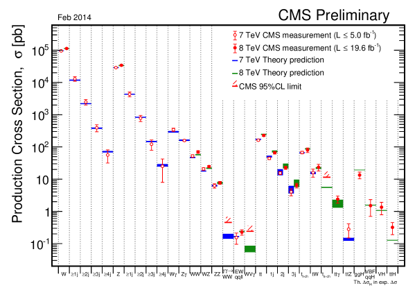
Figure 1: A compilation of cross sections at the LHC measured by the CMS Collaboration [1].

Of course, the highlight of Run 1 of the LHC was the discovery by CMS and ATLAS of a (the?) Higgs boson [2], whose production has by now been observed in three different production channels, as also seen in Fig. 1. The second highlight of Run 1 was the observation by LHCb and CMS of $B_{s}\to\mu^{+}\mu^{-}$ decay [3], again in agreement with the SM.

Lovers of physics beyond the Standard Model (BSM) have had to be patient so far, though Run 1 of the LHC has produced a few, not very significant, anomalies and excesses to get excited about, including in flavour physics. One of the focuses during Run 2 will be the more detailed study of the Higgs boson and probes whether its properties deviate from SM predictions, e.g., in the flavour sector. As I discuss later, the measurement of the Higgs mass has produced a new reason to expect BSM physics, and the search for BSM physics will start anew at Run 2, with its greatly increased centre-of-mass energy and increased integrated luminosity. My personal favourite candidate for BSM physics is supersymmetry (SUSY), and I also discuss later in this talk how SUSY models are constrained by flavour physics, as well as by the observations to date of the Higgs boson and searches for BSM physics with Run-1 data.

2 Higgs Physics

The most fundamental property of the Higgs boson is its mass , which can be measured most accurately in the $\gamma\gamma$ and $ZZ^{*}\to 2\ell^{+}2\ell^{-}$ final states. ATLAS and CMS report accurate measurements in both these final states. ATLAS measures [5]

$$H\to\gamma\gamma:m_{H} =\;125.98\pm 0.42\pm 0.28~{}{\rm GeV}=\;125.98\pm 0.50~{}{\rm GeV}\,,$$

$$H\to ZZ^{*}:m_{H} =\;125.51\pm 0.52\pm 0.04~{}{\rm GeV}=\;125.51\pm 0.52~{}{\rm GeV}\,,$$

$${\rm ATLAS~{}combined:}~{}m_{H} =\;125.36\pm 0.37\pm 0.18~{}{\rm GeV}\;=\;125.36\pm 0.41~{}{\rm GeV}\,,$$ (1)

and CMS measures [6]

$$H\to\gamma\gamma:m_{H} =\;124.70\pm 0.31\pm 0.15~{}{\rm GeV}\;=\;124.70^{+0.35}_{-0.34}~{}{\rm GeV}\,,$$

$$H\to ZZ^{*}:m_{H} =\;125.6\pm 0.4\pm 0.2~{}{\rm GeV}\,=\;125.6\pm 0.4~{}{\rm GeV}\,,$$

$${\rm CMS~{}combined:}~{}m_{H} =\;125.03^{+0.26}_{-0.27}~{}^{+0.13}_{-0.15}~{}{\rm GeV}\;=\;125.03\pm 0.30~{}{\rm GeV}\,.$$ (2)

Some interest has been generated by the differences in the masses measured in these channels, but these have opposite signs in the two experiments:

$${\rm ATLAS}:\;\Delta m_{H} =\;1.47\pm 0.67\pm 0.18~{}{\rm GeV}\,,$$

$${\rm CMS}:\;\Delta m_{H} =\;-0.9\pm 0.4\pm 0.2^{+0.34}_{-0.35}~{}{\rm GeV}\,,$$ (3)

so are presumably statistical and/or systematic artefacts. Combining naively the ATLAS and CMS measurements yields

$$m_{H}\;=\;125.15\pm 0.24~{}{\rm GeV}.$$ (4)

In addition to being a fundamental measurement in its own right, and casting light on the possible validity of various BSM models, the precise value of $m_{H}$ is also important for the stability of the electroweak vacuum in the Standard Model, as discussed later.

As seen in Fig. 2, the strengths of the Higgs signals measured by ATLAS and CMS individual channels are generally compatible with the SM predictions within the statistical fluctuations [7, 8], which are inevitably large at this stage. Combining their measurements in the $\gamma\gamma$, $ZZ^{*}$, $WW^{*}$, $b\bar{b}$ and $\tau^{+}\tau^{-}$ channels, ATLAS and CMS report the following overall signal strengths:

$${\rm ATLAS:}~{}\mu =\;1.30\pm 0.12\pm 0.10\pm 0.09\,,$$

$${\rm CMS:}~{}\mu =\;1.00\pm 0.09~{}^{+0.08}_{-0.07}\pm 0.07\,.$$ (5)

These averages are again quite compatible with each other and with the SM, and measurements at the Tevatron are also compatible with SM predictions for the Higgs boson [9].

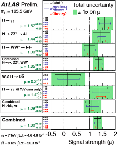
Figure 2: The Higgs signal strengths $\mu$, normalised to unity for the SM, as measured by ATLAS [7] (left panel) and CMS [8] (right panel).

One way to analyse the Higgs couplings is by allowing each one to differ from the SM prediction by individual factors $\kappa_{i}$ [10], and use the data to constrain these factors. In the case of the Higgs couplings to fermions, this is a direct way of probing its flavour properties. Within this general approach, it is also interesting to impose restrictions on the $\kappa_{i}$ that are motivated, e.g., by specific classes of composite models, and look for deviations from the SM that might arise in such models. Fig. 3 shows one such example [11], in which the $H$ couplings to the $W^{\pm}$ and $Z^{0}$ bosons are rescaled by a common factor $a$ and those to fermions by a common factor $c$. The data are completely consistent with the SM case $a=c=1$, indicated by the green star. The predictions of some specific composite models are indicated by yellow lines: some of these models are clearly incompatible with the data, and the survivors must be tuned to give predictions close to those of the SM.

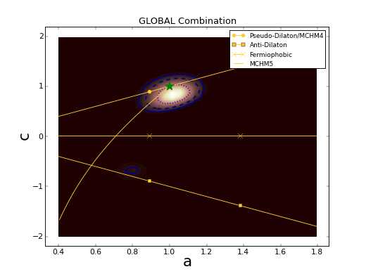
Figure 3: A global fit to bosonic and fermionic $H$ couplings rescaled by factors $a$ and $c$, respectively, showing the possible predictions of some composite models (yellow lines) and the SM (green star) [11].

It is a key prediction of the SM that the Higgs couplings to other particles should be related to their masses (linearly for fermions, quadratically for bosons), and this is indirectly verified by the measurements in Fig. 2. It is also possible to test this prediction directly, as seen in Fig. 4. Here we made a global fit to the data then available parametrising the Higgs couplings as [11]

$$\lambda_{f}\;=\;\sqrt{2}\left(\frac{m_{f}}{M}\right)^{(1+\epsilon)},\;\;g_{V}\;=\;2\left(\frac{M_{V}^{2(1+\epsilon)}}{M^{(1+\epsilon)}}\right)\,.$$ (6)

As seen in the left panel of Fig. 4, the data yielded

$$\epsilon\;=\;-0.022^{+0.020}_{-0.043},\;\;M\;=\;244^{+20}_{-10}~{}{\rm GeV},\,$$ (7)

quite compatible with the SM predictions $\epsilon=0$, $M=246$ GeV. It seems that, to a first approximation, Higgs couplings have the same flavour structure as particle masses. The right panel shows how accurately the ATLAS Collaboration estimates that it will be able to test the expected mass dependence of Higgs couplings with data from future runs of the LHC [12]. Let us see what Run 2 will bring.

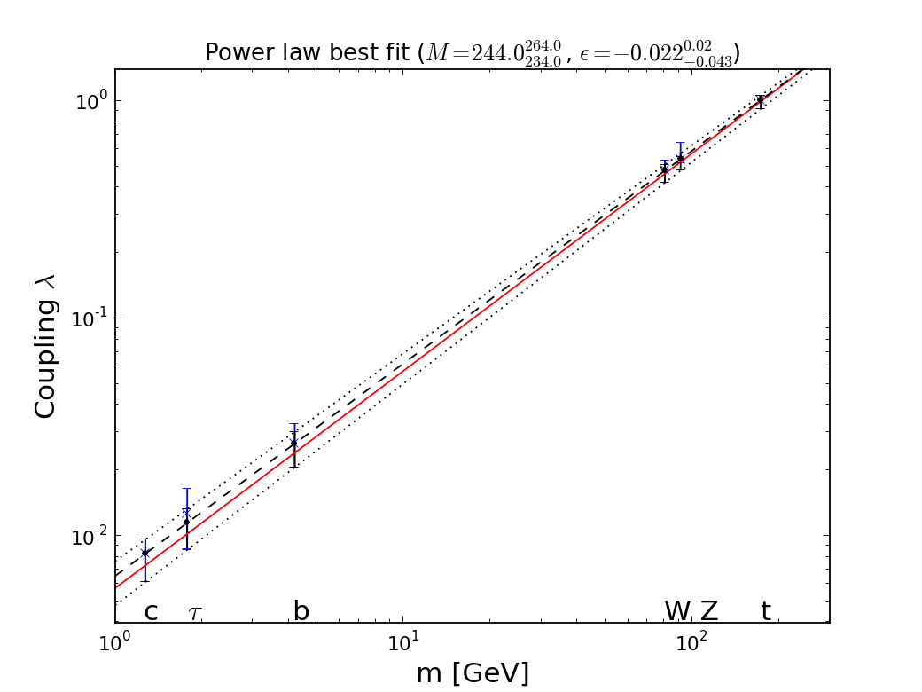
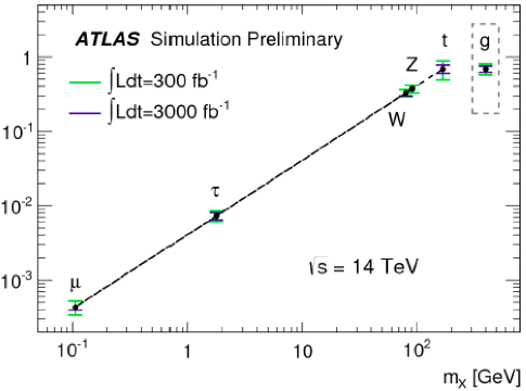
Figure 4: Left panel: A global fit to the $H$ couplings of the form (6), which is very compatible with the expected linear mass dependence for fermions and quadratic mass dependence for bosons (red line) [11]. Right panel: Preliminary simulation by ATLAS of prospective fits to the couplings’ mass dependence with future LHC data [12].

Going forward, a useful way to analyse Higgs and other electroweak data in a coherent way is to use an ‘effective SM parameterisation’ constructed in terms of SM fields, but including higher-dimensional operators that might arise from integrating out heavier degrees of freedom. This opens the way to the systematic study of electroweak precision tests and triple-gauge couplings (TGCs), as well as Higgs couplings, in a unified and efficient framework. Some results from a recent global analyses of the LHC Run 1 constraints on these observables is shown in Fig. 5 [13]. One finds that precision electroweak measurements, Higgs observables (including the kinematics of associated Higgs production) and TGCs play complementary rôles in constraining the coefficients of possible, pushing possible new physics beyond the TeV scale in some cases.

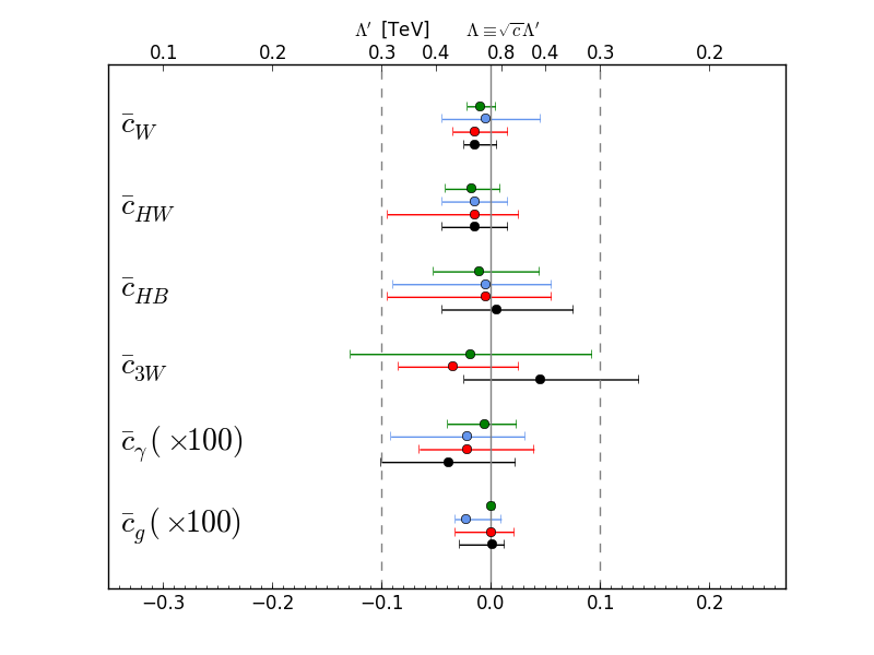
Figure 5: The 95% CL constraints on dimension-6 operators composed of SM fields, as obtained from single-coefficient fits (green bars), and the marginalised 95% ranges for the LHC signal-strength data combined with the kinematic distributions for associated $H+V$ production measured by ATLAS and D0 (blue bars), combined with the LHC TGC data (red lines), and the global combination with both the associated production and TGC data (black bars). From [13].

This effective field theory approach will surely be invaluable for analysing the data from LHC Run 2.

3 Flavour Physics

The Cabibbo-Kobayashi-Maskawa (CKM) description of flavour mixing and CP violation has made many successful predictions, and has passed most Run-1 tests with flying colours. In particular, it predicted successfully the branching ratio for the rare decay $B_{s}\to\mu^{+}\mu^{-}$ [3]:

$$BR(B_{s}\to\mu^{+}\mu^{-})\;=\;2.8^{+0.7}_{-0.6}\times 10^{-9}\,,$$ (8)

as seen in Fig. 6, which has been the second highlight of LHC Run 1. However, a point to watch during Run 2 will be the branching ratio for $B_{d}\to\mu^{+}\mu^{-}$ decay, whose ratio to $B_{s}\to\mu^{+}\mu^{-}$ is an ironclad prediction of the CKM model and models with minimal flavour violation (MFV), including many SUSY scenarios. As also seen in Fig. 6, the joint CMS and LHCb analysis has an indication of a $B_{d}\to\mu^{+}\mu^{-}$ signal that is considerably larger than the SM prediction:

$$BR(B_{d}\to\mu^{+}\mu^{-})\;=\;3.9^{+1.6}_{-1.4}\times 10^{-10}\,.$$ (9)

Could this indicate that MFV is not the whole story? Une affaire à suivre!

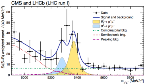
Figure 6: The signal for $B_{s}\to\mu^{+}\mu^{-}$ decay observed by the CMS and LHCb Collaborations [3], together with a hint of $B_{d}\to\mu^{+}\mu^{-}$ decay.

Despite the successes of the CKM paradigm, see the left panel of Fig. 7, there is scope for new physics beyond it, and some hints of cracks in its facade. For example, the data allow an important BSM contribution to the mixing amplitude for $B_{s}$ mesons: $A=A|_{SM}\times(1+h_{s}e^{i\sigma_{s}})$, as seen in the right panel of Fig. 7 [14]. Also, although the early indications of CP violation in $D$ decays above the CKM level have not been confirmed with more data, there a few intriguing anomalies. For example, the branching ratio for $B^{\pm}\to\tau^{\pm}\nu$ decay differs from the SM prediction by $\sim 2\sigma$, and there are issues with $e-\mu$ universality in semileptonic $B$ decays [15]. The most significant anomaly appears in the $P_{5}^{\prime}$ angular distribution for $B^{0}\to K^{*0}\mu^{+}\mu^{-}$ [16], though the nonperturbative corrections need to be understood better. Also worth noting are discrepancies in the determinations of the $V_{ub}$ CKM matrix element, and there is still an anomaly in the diimuon asymmetry at the Tevatron [17].

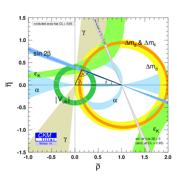
Figure 7: Left panel: Flavour and CP violation measurements generally agree well with the CKM paradigm. Right panel: Experimental constraint on a possible non-Standard Model contribution to $B_{s}$ mixing [14].

Some anomalies do seem to be going away, such as the forward-backward asymmetry in $t\bar{t}$ production, which now agrees with higher-order QCD calculations [18], as does the $t\bar{t}$ rapidity asymmetry measured at the LHC. However, there are plenty of flavour issues to be addressed during LHC Run 2.

One of the key predictions of the SM, which also holds in many SUSY models, is that the Higgs couplings to fermions should conserve flavour to a very good approximation, and this is consistent with the upper limits on low-energy effective flavour-changing interactions. However, these would allow lepton-flavour-violating Higgs couplings to fermions far above the SM predictions, so looking for such interactions is a possible window on BSM physics. Specifically, we found that the branching ratios for $H\to\mu\tau$ and $H\to e\tau$ decays could each be as large as ${\cal O}(10)$%, whereas the branching ratio for $H\to\mu e$ must be $\lesssim 10^{-5}$ [19]. The CMS Collaboration has recently searched for $H\to\mu\tau$ decays in various $H$ production modes, as seen in Fig. 8, and found [20]

$${\rm BR}(H\to\mu\tau)\;=\;0.89^{+0.40}_{-0.37}\,\%\,,$$ (10)

which has a background-only $p$-value of 0.007, corresponding to 2.46$\sigma$. On the one hand, this tells us that Higgs measurements are already probing flavour physics beyond the previous low-energy experiments and, on the other hand, it will be very interesting to see corresponding results from ATLAS and results from Run 2!

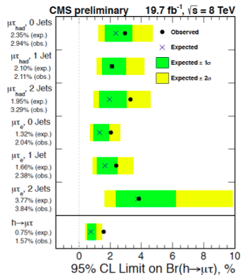
Figure 8: Results from the CMS search for $H\to\mu\tau$ decay [20].

It will also be interesting to see whether the Higgs couplings contain CP-odd admixtures. We already know that its couplings to massive gauge bosons are predominantly CP-even, but we have very little direct information about its couplings to fermions, though there have been suggestions how to measure the CP properties of the $H\tau^{+}\tau^{-}$ coupling, for example. How about the $Ht{\bar{t}}$ coupling? There are indirect constraints from the available experimental information on the $Hgg$ and $H\gamma\gamma$ couplings, as seen in the left panel of Fig. 9. Direct information could come in the future from measurements of the cross sections for associated ${\bar{t}}tH$, $tH$ and ${\bar{t}}H$ production, which are sensitive to $\zeta_{t}\equiv\arg({\rm CP-odd~{}coupling}/{\rm CP-even~{}coupling})$, as seen in Fig. 9 [21]. One could also look for CP-violating final-state asymmetries in $t({\bar{t}})$ decays. A challenge for Run 2 and beyond!

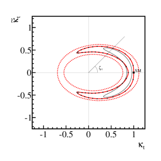
Figure 9: Left panel: The constraints on the CP-even and -odd $Ht{\bar{t}}$ couplings from measurements of the $Hgg$ and $H\gamma\gamma$ couplings. Right panel: The dependences of the cross sections for associated ${\bar{t}}tH$, $tH$ and ${\bar{t}}H$ production, on $\zeta_{t}\equiv\arg({\rm CP-odd~{}coupling}/{\rm CP-even~{}coupling})$. From [21].

4 The SM is not enough!

Now that the SM has apparently been completed by the discovery of a (the?) Higgs boson, some might argue that there is no physics beyond the SM. However, history is lettered with distinguished physicists (and others) who declared “game over” prematurely. Albert Michelson declared in 1894 that “The more important fundamental laws and facts of physical science have all been discovered”, just before the discoveries of radioactivity and the electron. Lord Kelvin declared in 1900 that “There is nothing new to be discovered in physics now, all that remains is more and more precise measurement”, just before Einstein postulated the photon and proposed special relativity.

There are many reasons why the SM is not enough. Inspired by James Bond [22], here I just mention 007 of them. 1) Taking at face value the measured values of $m_{t}$ and $m_{H}$, the electroweak vacuum is probably unstable, unless additional physics intervenes. 2) The dark matter required by astrophysics and cosmology cannot be provided by the SM. 3) The origin of matter in the Universe requires addition CP violation beyond the CKM model. 4) Explaining the small sizes of the neutrino masses requires physics beyond the SM. 5) The hierarchy and fine-tuning problems suggest there is new physics at the TeV scale. 6) Cosmological inflation (probably) requires physics beyond the SM, in particular because the effective Higgs potential is probably negative at high scales, as discussed shortly. 7) The construction of a consistent quantum theory of gravity certainly involves going (far) beyond the SM.

5 New Reasons to Love SUSY

Most of these issues would be at least alleviated by supersymmetry, and the LHC Run 1 has given us at least three new reasons to love SUSY, as I now discuss.

5.1 The Instability of the Electroweak Vacuum

In the SM the effective electroweak potential resembles a Mexican hat, invariant under the SM SU(2)$\times$U(1) symmetry, but unstable at the origin. The electroweak vacuum lies in a surrounding valley where $\langle H\rangle\equiv v=246$ GeV. Beyond this valley, the brim of the hat rises, but how far? Calculations show that renormalization by the top quark overwhelms that by the Higgs itself, for the measured values of $m_{t}$ and $m_{H}$, turning the brim down at large field values. Consequently, the present electroweak vacuum is in principle unstable, potentially collapsing into an anti-de-Sitter ’Big Crunch’ via quantum tunnelling though the brim.

According to the best SM calculations available, shown in the left panel of Fig. 10, the brim turns down at a Higgs scale $\Lambda$ [23]:

$$\log_{10}\left(\frac{\Lambda}{{\rm GeV}}\right)\;=\;11.3+1.0\left(\frac{m_{H}}{{\rm GeV}}-125.66\right)-1.2\left(\frac{m_{t}}{{\rm GeV}}-173.10\right)+0.4\left(\frac{\alpha_{s}(M_{Z})-0.1184}{0.0007}\right)\,.$$ (11)

Using the official world average values of $m_{t}$, $m_{H}$ and $\alpha_{s}(M_{Z})$, one may estimate

$$\Lambda\;=\;10^{10.5\pm 1.1}~{}{\rm GeV}$$ (12)

though the error is neither Gaussian nor symmetric. As seen in the right panel of Fig. 10, this calculation is most sensitive to $m_{t}$. Subsequent to the determination of the world average, D0 has reported a new, higher, value of $m_{t}$ [24], which would tend to decrease $\log_{10}(\Lambda/{\rm GeV})$ by 2.0, further destabilising the electroweak vacuum, but CMS has reported new analyses of $m_{t}$ [25] that would increase $\log_{10}(\Lambda/{\rm GeV})$ by 1.6, making the vacuum more stable. A more accurate value of $m_{t}$ would fix the fate of the Universe within the SM. However, the experimental effort must be matched by better theoretical understanding of the relationship between the effective mass parameter used by experiments in their Monte Carlos and the parameter $m_{t}$ in the SM Lagrangian [26].

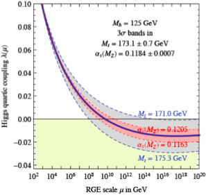
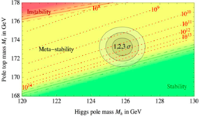
Figure 10: Left panel: Within the SM, normalisation by the top quark appears to drive the Higgs self-coupling $\lambda<0$. Right panel: The regions of vacuum stability, metastability and instability in the $(m_{H},m_{t})$ plane. Both panels are from [23].

In much of the favoured parameter space, the electroweak vacuum would (probably) live longer than the age of the Universe, so you might be tempted to shrug your shoulders, but there is another problem. Observations of the cosmic microwave background suggest that the Universe once had a very higher energy density during an inflationary epoch [27]. Quantum and thermal fluctuations during this epoch would have favoured a transition away from the electroweak minimum and towards an anti-de-Sitter ‘Big Crunch’ region [28]. One could argue that a non-anti-de-Sitter region containing us might have survived. Alternatively, the problem could be avoided in the presence of higher-dimensional terms in the effective potential [29]. This is just one example of new physics beyond the SM that could have averted this cosmological disaster: another is supersymmetry, which would have prevented the brim of the Mexican hat from turning down in the first place.

5.2 The Higgs Mass

It is well known that SUSY predicted correctly that the mass of the Higgs boson should be $\lesssim 130$ GeV in simple models [30]. This is because SUSY specifies the quartic Higgs coupling before renormalisation. Loop corrections to $m_{H}$ due (in particular) to $m_{t}$ increase it significantly, but are under control and accurate to with an estimated uncertainty of $\pm 3$ GeV for given values of the SUSY input parameters [31].

5.3 Higgs Couplings

Since there are two physical neutral CP-even Higgs bosons in the minimal SUSY extension of the SM (MSSM), and a neutral CP-even boson $A$ that could mix with them in the presence of CP violation, the couplings of the discovered Higgs boson could, in principle, have differed significantly from those of the SM Higgs boson. However, since around 2001 it has been known [32] that constraints from LEP and $b\to s\gamma$ already implied within simple SUSY models that the Higgs couplings would be very similar to those in the SM, as observed.

In the cases of contemporary best fits to the LHC and other data within simple SUSY models with all SUSY-breaking parameters constrained to be equal at the GUT scale (the CMSSM), or allowing one or two degrees of non-universality in the soft SUSY-breaking contributions to Higgs masses (NUHM1 and NUHM2), one finds that Higgs couplings should be much closer to the SM predictions than the experimental and theoretical uncertainties would allow. As seen in Fig. 11, it would require a high-luminosity circular $e^{+}e^{-}$ collider to distinguish these model predictions from the SM [33].

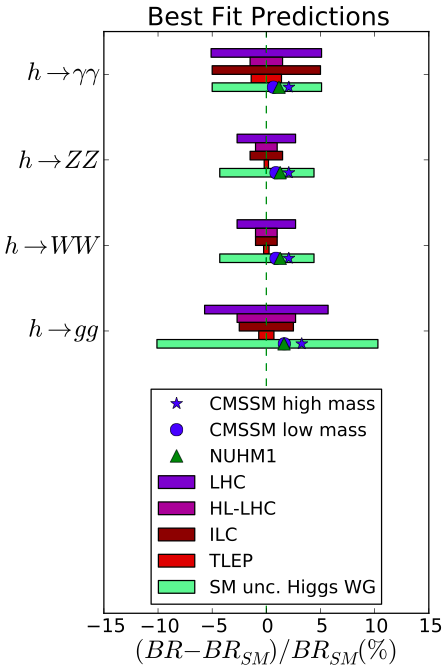
Figure 11: Comparison of the present precisions in measurements of various Higgs branching ratios, prospective measurements at future colliders, the current theoretical uncertainties, and the (small) deviations from the SM predictions found at the best-fit points in various SUSY models. From [33].

5.4 Not forgetting …

… the many reasons for loving SUSY established earlier, such as alleviating the fine-tuning aspect of the hierarchy problem, providing a natural candidate for the cold dark matter, facilitating grand unification and playing an essential rôle in string theory. It would be a shame if Nature did not succumb to SUSY’s manifold charms.

6 Supersymmetry

Despite our ardent love for SUSY, so far she has been very coy. Direct searches for SUSY at the LHC have drawn blanks so far. This is also the case for searches for the scattering of dark matter particles, indirect searches in flavour physics, etc.. The results of global fits to the CMSSM, NUHM1 and NUHM2, combining these constraints and requiring that the relic supersymmetric particle density be within the cosmological range, are shown projected on the $(m_{0},m_{1/2})$ plane in the left panel of Fig. 12 [34, 35]. The right panel of Fig. 12 displays the $(m_{\tilde{q}},m_{\tilde{g}})$ plane, showing prospective exclusion and discovery reaches of the LHC in future runs with 300 and 3000/fb of luminosity at high energy [12]. Superposed on this plane are the 68 and 95% CL contours found in the global fit to the CMSSM. As already seen in the left panel of Fig. 12, there are two distinct regions, the lower-mass one being favoured by the disagreement between experiment and the SM prediction of $g_{\mu}-2$. We see that the LHC could detect squarks and gluinos if Nature is described by supersymmetry with parameters in this lower-mass region.

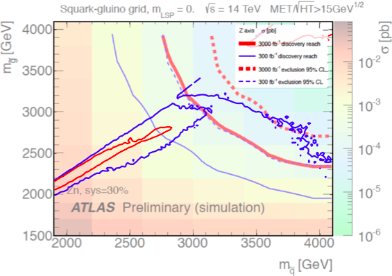
Figure 12: Left panel: The 68% CL (red) and 95% CL contours (blue) in the $(m_{0},m_{1/2})$ panes for the CMSSM (dotted lines), NUHM1 (dashed lines) and NUHM2 (solid lines) [35]. Right panel: The reach of ATLAS in the $(m_{\tilde{q}},m_{\tilde{g}})$ plane for exclusion and discovery with 300 and 3000/fb of integrated LHC liminosity at high energy [12], compared with the 68% CL (red) and 95% regions in the CMSSM.

Run 1 of the LHC imposed strong limits on strongly-interacting sparticles, whereas the limits on electroweakly-interacting sparticles are significantly weaker. It is only in models with universality imposed on the soft SUSY-breaking contributions to sparticle masses that the squark and gluino limits lead to strong limits on the masses of electroweakly-interacting sparticles. One may, instead, consider the phenomenological MSSM (pMSSM) in which no universality is assumed. In this case, the the lower limits on the gluino and squark masses are reduced, compared with the CMSSM, NUHM1 and NUHM2, as seen in Fig. 13, enhancing the prospects for discovering SUSY in LHC Run 2 [35].

Figure 13: The one-dimensional $\chi^{2}$ likelihood function for the mass of the gluino (left panel) and the right-handed squark (right panel) in the CMSSM, NUHM1, NUHM2 and pMSSM [35].

One intriguing feature of the pMSSM is that the decoupling of the masses of the strongly- and electroweakly-interacting sparticles revives the possibility that supersymmetry could explain the discrepancy between the experimental measurement of $g_{\mu}-2$ and the value calculated in the SM. As seen in the left panel of Fig. 14, the LHC constraints imply that the CMSSM, NUHM1 and NUHM2 all predict values of the $g_{\mu}-2$ that are very similar to the SM prediction, whereas the pMSSM could accommodate the experimental measurement. It is good that two new experiments to measure $g_{\mu}-2$ are being planned [36], and that other experiments will enable the SM predictions to be refined and hence the discrepancy between the SM and experiment to be clarified.

Figure 14: The one-dimensional $\chi^{2}$ likelihood function for $g_{\mu}-2$ (left panel) and $B_{s}\to\mu^{+}\mu^{-}$ (right panel) in the CMSSM, NUHM1, NUHM2 and pMSSM [35].

On the other hand, as seen in the right panel of Fig. 14, all of the CMSSM, NUHM1, NUHM2 and pMSSM can accommodate the experimental measurement of $B_{s}\to\mu^{+}\mu^{-}$. Interestingly, the pMSSM is the only one of these models that could yield a value of the branching ratio for this decay that is any lower than in the SM.

There have been spikes of interest in a couple of hints in the Run 1 data of signals that might be due to the production of electroweak sparticles. One was an apparent enhancement of the $W^{+}W^{-}$ cross section above the SM prediction [37], and the other was a possible ‘edge’ effect in the $\mu^{+}\mu^{-}$ invariant-mass distribution found by CMS [38]. However, the significance of the $W^{+}W^{-}$ cross-section discrepancy is much reduced when NNLO QCD effects are taken into account [39], and the dilepton edge effect should be given the opportunity to grow when more data are accumulated. Let us wait to see what Run 2 of the LHC brings.

7 Theoretical Perplexity

On the one hand, the discovery of a (the?) Higgs boson during Run 1 of the LHC has been a subject for rejoicing. On the other hand, the absence of any hard direct evidence for new physics beyond the SM, coupled with the apparently (bog) standard nature of the Higgs, has left theorists perplexed which BSM horse to back. (For the experimentalists, it is clear: more energy and more luminosity!)

Despite the lack of any evidence for SUSY, I would say that it has fared less badly than some rival theories. For example, generic composite models could have accommodated differences fem SM Higgs properties that are larger than those allowed by Run 1 data, whereas SUSY predicted successfully both its mass and the SM-ness of its couplings. Siren voices may sing the praises of split SUSY, high-scale SUSY, modifying or abandoning naturalness, or embracing the string landscape. My point of view, however, while admitting the need for new ideas, is that SUSY anywhere is better than SUSY nowhere. Let us see what Run 2 brings!

Perhaps the most significant hint from LHC Run 1 has been the fact that $(m_{H},m_{t})$ apparently lie within the zone where extrapolation to high scales indicates that the electroweak vacuum is unstable - though close to the boundary between the zones of stability and instability. If these parameters do indeed lie within the unstable region, this would provide a strong argument for new physics, as discussed earlier. On the other hand, if these masses do lie on or close to the stability boundary, perhaps there is some critical phenomenon to be understood? We trust that Run 2 will clarify where we are located in the $(m_{H},m_{t})$ plane.

8 Patience!

After its proposal, it took 48 years for the Higgs boson to be discovered, a time-lag that was longer than those between the proposals and discoveries of other elementary particles [40]. So lovers of SUSY can be patient. At the time of writing, only 41 years have passed since the first proposal of four-dimensional supersymmetric field theories. If SUSY is discovered during LHC Run 2 or 3, the SUSY time-lag will be less than that for the Higgs boson. Let us see what happens when the LHC restarts!

References

- [1] CMS Collaboration, https://twiki.cern.ch/twiki/bin/view/CMSPublic/PhysicsResultsSMP.
- [2] G. Aad et al. [ATLAS Collaboration], Phys. Lett. B 716 (2012) 1 [arXiv:1207.7214 [hep-ex]]; S. Chatrchyan et al. [CMS Collaboration], Phys. Lett. B 716 (2012) 30 [arXiv:1207.7235 [hep-ex]].
- [3] V. Khachatryan et al. [CMS and LHCb Collaborations], arXiv:1411.4413 [hep-ex] and references therein.
- [4] G. Aad et al. [ATLAS Collaboration], Phys. Lett. B 726 (2013) 120 [arXiv:1307.1432 [hep-ex]]; V. Khachatryan et al. [CMS Collaboration], arXiv:1411.3441 [hep-ex].
- [5] G. Aad et al. [ATLAS Collaboration], Phys. Rev. D 90 (2014) 052004 [arXiv:1406.3827 [hep-ex]].
- [6] CMS Collaboration, http://cds.cern.ch/record/1728249/files/HIG-14-009-pas.pdf.
- [7] ATLAS Collaboration, https://twiki.cern.ch/twiki/bin/view/AtlasPublic/HiggsPublicResults.
- [8] S. Chatrchyan et al. [CMS Collaboration], JHEP 1306 (2013) 081 [arXiv:1303.4571 [hep-ex]].
- [9] CDF and D0 Collaborations, http://tevnphwg.fnal.gov.
- [10] A. David et al. [LHC Higgs Cross Section Working Group Collaboration], arXiv:1209.0040 [hep-ph].
- [11] J. Ellis and T. You, JHEP 1306 (2013) 103 [arXiv:1303.3879 [hep-ph]].
- [12] ATLAS Collaboration, arXiv:1307.7292 [hep-ex].
- [13] J. Ellis, V. Sanz and T. You, arXiv:1410.7703 [hep-ph] and references therein.
- [14] J. Charles, S. Descotes-Genon, Z. Ligeti, S. Monteil, M. Papucci and K. Trabelsi, Phys. Rev. D 89 (2014) 033016 [arXiv:1309.2293 [hep-ph]].
- [15] R. Aaij et al. [LHCb Collaboration], Phys. Rev. Lett. 113 (2014) 151601 [arXiv:1406.6482 [hep-ex]].
- [16] R. Aaij et al. [LHCb Collaboration], Phys. Rev. Lett. 111 (2013) 19, 191801 [arXiv:1308.1707 [hep-ex]].
- [17] V. M. Abazov et al. [D0 Collaboration], Phys. Rev. Lett. 105 (2010) 081801 [arXiv:1007.0395 [hep-ex]].
- [18] T. Aaltonen et al. [CDF Collaboration], Phys. Rev. D 87 (2013) 9, 092002 [arXiv:1211.1003 [hep-ex]].
- [19] G. Blankenburg, J. Ellis and G. Isidori, Phys. Lett. B 712 (2012) 386 [arXiv:1202.5704 [hep-ph]].
- [20] CMS Collaboration, https://cds.cern.ch/record/1740976?ln=en.
- [21] J. Ellis, D. S. Hwang, K. Sakurai and M. Takeuchi, JHEP 1404 (2014) 004 [arXiv:1312.5736 [hep-ph]].
- [22] J. Bond et al., http://www.imdb.com/title/tt0143145/.
- [23] D. Buttazzo, G. Degrassi, P. P. Giardino, G. F. Giudice, F. Sala, A. Salvio and A. Strumia, JHEP 1312 (2013) 089 [arXiv:1307.3536].
- [24] A. Jung, on behalf of the D0 Collaboration, https://indico.cern.ch/event/279518/session/27/contribution/36/ material/slides/0.pdf.
- [25] CMS Collaboration, http://cds.cern.ch/record/1951019/files/TOP-14-015-pas.pdf.
- [26] S. Moch, S. Weinzierl, S. Alekhin, J. Blumlein, L. de la Cruz, S. Dittmaier, M. Dowling and J. Erler et al., arXiv:1405.4781 [hep-ph].
- [27] P. A. R. Ade et al. [Planck Collaboration], Astron. Astrophys. 571 (2014) A22 [arXiv:1303.5082 [astro-ph.CO]]; P. A. R. Ade et al. [BICEP2 Collaboration], Phys. Rev. Lett. 112 (2014) 241101 [arXiv:1403.3985 [astro-ph.CO]].
- [28] M. Fairbairn and R. Hogan, Phys. Rev. Lett. 112 (2014) 201801 [arXiv:1403.6786 [hep-ph]]; A. Hook, J. Kearney, B. Shakya and K. M. Zurek, arXiv:1404.5953 [hep-ph].
- [29] V. Branchina, E. Messina and M. Sher, arXiv:1408.5302 [hep-ph].
- [30] J. R. Ellis, G. Ridolfi and F. Zwirner, Phys. Lett. B 257 (1991) 83; H. E. Haber and R. Hempfling, Phys. Rev. Lett. 66 (1991) 1815; Y. Okada, M. Yamaguchi and T. Yanagida, Prog. Theor. Phys. 85 (1991) 1.
- [31] T. Hahn, S. Heinemeyer, W. Hollik, H. Rzehak and G. Weiglein, Phys. Rev. Lett. 112 (2014) 14, 141801 [arXiv:1312.4937 [hep-ph]].
- [32] J. R. Ellis, S. Heinemeyer, K. A. Olive and G. Weiglein, Phys. Lett. B 515 (2001) 348 [hep-ph/0105061].
- [33] M. Bicer et al. [TLEP Design Study Working Group Collaboration], JHEP 1401 (2014) 164 [arXiv:1308.6176 [hep-ex]].
- [34] O. Buchmueller, R. Cavanaugh, M. Citron, A. De Roeck, M. J. Dolan, J. R. Ellis, H. Flaecher and S. Heinemeyer et al., arXiv:1408.4060 [hep-ph].
- [35] O. Buchmueller, R. Cavanaugh, M. Citron, A. De Roeck, M. J. Dolan, J. R. Ellis, H. Flaecher and S. Heinemeyer et al., The pMSSM after LHC Run 1, in preparation.
- [36] FNAL g-2 Collaboration, http://muon-g-2.fnal.gov; H. Iinuma (for the J-PARC New g-2/EDM experiment collaboration), http://iopscience.iop.org/1742-6596/295/1/012032/pdf/ 1742-6596_295_1_012032.pdf.
- [37] K. Rolbiecki and K. Sakurai, JHEP 1309 (2013) 004 [arXiv:1303.5696 [hep-ph]]; D. Curtin, P. Meade and P. J. Tien, arXiv:1406.0848 [hep-ph]; J. S. Kim, K. Rolbiecki, K. Sakurai and J. Tattersall, arXiv:1406.0858 [hep-ph].
- [38] CMS Collaboration, http://cds.cern.ch/record/1751493/files/SUS-12-019-pas.pdf.
- [39] T. Gehrmann, M. Grazzini, S. Kallweit, P. Maierhöfer, A. von Manteuffel, S. Pozzorini, D. Rathlev and L. Tancredi, arXiv:1408.5243 [hep-ph].
- [40] http://www.economist.com/blogs/graphicdetail/2012/07/daily-chart-1.