On the optimal estimates and comparison of Gegenbauer expansion coefficients

Abstract

In this paper, we study optimal estimates and comparison of the coefficients in the Gegenbauer series expansion. We propose an alternative derivation of the contour integral representation of the Gegenbauer expansion coefficients which was recently derived by Cantero and Iserles [SIAM J. Numer. Anal., 50 (2012), pp.307–327]. With this representation, we show that optimal estimates for the Gegenbauer expansion coefficients can be derived, which in particular includes Legendre coefficients as a special case. Further, we apply these estimates to establish some rigorous and computable bounds for the truncated Gegenbauer series. In addition, we compare the decay rates of the Chebyshev and Legendre coefficients. For functions whose singularity is outside or at the endpoints of the expansion interval, asymptotic behaviour of the ratio of the $n$th Legendre coefficient to the $n$th Chebyshev coefficient is given, which provides us an illuminating insight for the comparison of the spectral methods based on Legendre and Chebyshev expansions.

Keywords: Gegenbauer coefficients, optimal estimates, error bounds, Legendre coefficients, Chebyshev coefficients.

AMS classifications: 41A10, 41A25, 65N35.

1 Introduction

Gegenbauer polynomials together with their special cases like Legendre and Chebyshev polynomials are widely used in many branches of numerical analysis such as interpolation and approximation theories, the construction of quadrature formulas, the resolution of Gibbs phenomenon and spectral and pseudo-spectral methods for ordinary and partial differential equations. One of the most attractive features is that these families of orthogonal polynomials have excellent error properties in the approximation of a globally smooth function. Typically, the error of the truncated series in Gegenbauer polynomials decreases exponentially fast for analytic functions as the number of the series increases. For entire functions, the error will decrease even faster than exponential. This remarkable property explains why Gegenbauer and its special cases are extensively used to solve various problems arising from science and engineering.

Let $C_{k}^{(\lambda)}(x)$ denote the Gegenbauer polynomial of degree $k$ which is normalized by the following condition

$$C_{k}^{(\lambda)}(1)=\frac{\Gamma(k+2\lambda)}{k!\Gamma(2\lambda)},$$ (1.1)

where $\lambda>-\frac{1}{2}$ and $\lambda\neq 0$. For the special case $\lambda=0$, we have

$$C_{k}^{(0)}(1)=\frac{2}{k},\quad k\geq 1,$$

and $C_{0}^{(0)}(x)=1$. For a fixed $\lambda$, these Gegenbauer polynomials are orthogonal over the interval $[-1,1]$ with respect to the weight function $\omega(x)=(1-x^{2})^{\lambda-\frac{1}{2}}$ and

$$\int_{-1}^{1}(1-x^{2})^{\lambda-\frac{1}{2}}C_{m}^{(\lambda)}(x)C_{n}^{(\lambda)}(x)dx=h_{n}^{(\lambda)}\delta_{mn},$$ (1.2)

where $\delta_{mn}$ is the Kronnecker delta and

$$h_{n}^{(\lambda)}=\frac{2^{1-2\lambda}\pi}{\Gamma(\lambda)^{2}}\frac{\Gamma(n+2\lambda)}{\Gamma(n+1)(n+\lambda)},\quad\lambda\neq 0.$$ (1.3)

For applications in numerical analysis, it is often required to expand a given function $f(x)$ in terms of Gegenbauer polynomials as

$$f(x)=\sum_{n=0}^{\infty}a_{n}^{\lambda}C_{n}^{(\lambda)}(x),$$ (1.4)

where the Gegenbauer coefficients are defined by

$$a_{n}^{\lambda}=\frac{1}{h_{n}^{(\lambda)}}\int_{-1}^{1}(1-x^{2})^{\lambda-\frac{1}{2}}f(x)C_{n}^{(\lambda)}(x)dx,\quad n\geq 0.$$ (1.5)

The Gegenbauer expansion (1.4) is an invaluable and powerful tool in a wide range of practical applications. In particular, they are widely used in the resolution of Gibbs phenomenon and numerical solutions of ordinary and partial differential equations (see, for example, [4, 13, 14, 15, 16, 17, 19, 26]). In these applications, it is frequently required to estimate the error bound of the truncated Gegenbauer expansion in the uniform norm. It is well known that the error of the truncated spectral expansion depends solely on how fast the corresponding spectral expansion coefficients decay. Therefore, the final aim is reduced to the estimate of decay rate of the corresponding spectral coefficients.

For the Gegenbauer coefficients, the estimate of their decay rate was received attention in the past few decades and some results have been developed in the literatures. For example, to defeat the Gibbs phenomenon, Gottlieb and Shu in a number of papers [13, 14, 15, 16, 17] proposed to reexpand the truncated Fourier or Chebyshev series into a Gegenbauer series. To prove the exponential convergence of the Gegenbauer series, a rough estimate of the Gegenbauer coefficients was proposed (see [17, Eqn. (4.3)]). More recently, this issue was considered in [32, 33] and some sharper estimates were given. In these works, the main idea is to express the Gegenbauer coefficient $a_{n}^{\lambda}$ as an infinite series either by using the Chebyshev expansion of the first kind of $f$ or the Cauchy integral formula together with the generating function of the Chebyshev polynomial of the second kind, and then estimate the derived infinite series term by term. As we shall see, these results are often overestimated. For special cases of the Gegenbauer spectral expansion such as Chebyshev and Legendre expansions, the estimates of their expansion coefficients have been studied extensively in the past few decades (see [3, 5, 8, 10, 31, 32, 33] and references therein).

In this article we will develop a novel approach to study the estimate of the Gegenbauer coefficients. The starting point of our analysis is the contour integral expression which was recently derived by Cantero and Iserles in [7]. Their idea was based on expressing the Gegenbauer coefficients in terms of an infinite linear combination of derivatives at the origin and then by an integral transform with a Gauss hypergeometric function as its kernel. This kernel function converges too slowly to be computationally useful. To remedy this, a hypergeometric transformation was proposed to replace the original kernel by a new one which converges rapidly. This, to the author’s knowledge, is the first result on the contour integral expression of the Gegenbauer coefficients. However, as the authors admit in their paper [7, 20], the proof of their derivation is rather convoluted.

Here, we shall provide an alternative and simple approach to derive the contour integral expression of the Gegenbauer coefficients. Our idea is motivated by the connection formula between the Gegenbauer and Chebyshev polynomials of the second kind, which was initiated in [30]. We show that the contour integral expression of the Gegenbauer coefficients can be derived by rearranging the Chebyshev coefficients of the second kind. With the derived contour integral expression in hand, we prove that optimal estimates for the Gegenbauer coefficients can be obtained as direct consequences. To the best of our knowledge, these are the first results of this kind that are proved to be optimal. In contrast to existing studies, numerical results indicate that our estimates are superior. Further, we apply these estimates to establish some rigorous and computable bounds for the truncated Gegenbauer series in the uniform norm.

Among the families of Gegenbauer spectral expansions, Chebyshev and Legendre expansions are the most popular and important cases (see [2, 26, 29]). One particularly interesting question for these two expansions is the comparison of the decay rates of the Legendre and Chebyshev coefficients. This issue was considered by Lanczos in [22] and later by Fox and Parker in [11], where these authors deduced that the $n$th Chebyshev coefficient decays approximately $\sqrt{n\pi}/2$ faster than its Legendre counterpart. Very recently, Boyd and Petschek in [6] checked this issue carefully and showed that this assertion is not true for some concrete examples. In this work, with the help of the contour integral expression of Gegenbauer coefficients, we improve significantly the observation stated in [6] and present delicate results on the comparison of the Legendre and Chebyshev coefficients. More precisely, for functions whose singularity is outside the interval $[-1,1]$, the asymptotic behaviour of the ratio $\gamma_{n}=a_{n}^{L}/a_{n}^{C}$, where $a_{n}^{L}$ and $a_{n}^{C}$ denote the $n$th Legendre and Chebyshev coefficient of $f$ respectively, is derived which shows that the above assertion by Lanczos and Fox and Parker is always false if the singularity is finite. We also extend our results to functions with endpoint singularity and subtle results on the asymptotic behaviour of $\gamma_{n}$ are given.

This paper is organized as follows. In the next section, we collect some well known properties of Gegenbauer polynomials which will be used in the later sections. In section 3, we provide an alternative way to derive the contour integral expression of Gegenbauer coefficients. With the contour integral expression obtained, in section 4 we present optimal estimates of the Gegenbauer coefficients and apply these to derive error bounds of the truncated Gegenbauer expansion in the uniform norm. A comparison of the Legendre and Chebyshev coefficients are discussed in section 5. Finally, in section 6 we give some final remarks .

2 Some properties of Gegenbauer polynomials

In this section we will collect some well-known properties of Gegenbauer polynomials which will be used in the subsequent analysis. All these properties can be found in [27].

Gegenbauer polynomials satisfy the following three-term recurrence relation

$$(n+1)C_{n+1}^{(\lambda)}(x)=2x(n+\lambda)C_{n}^{(\lambda)}(x)-(n+2\lambda-1)C_{n-1}^{(\lambda)}(x),\quad n\geq 1,$$ (2.1)

where $C_{0}^{(\lambda)}(x)=1$ and $C_{1}^{(\lambda)}(x)=2\lambda x$. These polynomials also satisfy the following symmetry relations

$$C_{n}^{(\lambda)}(x)=(-1)^{n}C_{n}^{(\lambda)}(-x),\quad n\geq 0,$$ (2.2)

which imply that $C_{n}^{(\lambda)}(x)$ is an even function for even $n$ and an odd function for odd $n$. Moreover, Gegenbauer polynomials satisfy the following inequality

$$|C_{n}^{(\lambda)}(x)|\leq C_{n}^{(\lambda)}(1),\quad|x|\leq 1,~{}~{}\lambda>0,~{}~{}n\geq 0.$$ (2.3)

Gegebauer polynomials include some important polynomials such as Legendre and Chebyshev polynomials as special cases. More specifically, we have

$$P_{n}(x)=C_{n}^{(\frac{1}{2})}(x),\quad U_{n}(x)=C_{n}^{(1)}(x),\quad n\geq 0,$$ (2.4)

where $P_{n}(x)$ is the Legendre polynomial of degree $n$ and $U_{n}(x)$ is the Chebyshev polynomial of the second kind of degree $n$. When $\lambda=0$, the Gegenbauer polynomials reduce to the Chebyshev polynomials of the first kind by the following definition

$$\lim_{\lambda\rightarrow 0^{+}}\lambda^{-1}C_{n}^{(\lambda)}(x)=\frac{2}{n}T_{n}(x),\quad n\geq 1,$$ (2.5)

where $T_{n}(x)$ is the Chebyshev polynomial of the first kind of degree $n$.

3 A simple derivation of contour integral expression for Gegenbauer coefficients

In this section we shall present a new and simple derivation of the contour integral expression of Gegenbauer coefficients. Our idea is based on the connection formula between the Gegenbauer polynomial and the Chebyshev polynomial of the second kind.

Lemma 3.1.

We have

$$C_{n}^{(\lambda)}(x)=\sum_{k=0}^{\left\lfloor\frac{n}{2}\right\rfloor}\frac{(\lambda)_{n-k}(\lambda-\mu)_{k}(n+\mu-2k)}{(\mu+1)_{n-k}k!\mu}C_{n-2k}^{(\mu)}(x),$$ (3.1)

where $\lfloor\cdot\rfloor$ denotes the integer part.

Proof.

See [1, p. 360]. ∎

Based on the above lemma, we are now able to derive the contour integral expression of Gegenbauer coefficients. Before that, we introduce the Bernstein ellipse $\mathcal{E}_{\rho}$ which is defined by

$$\mathcal{E}_{\rho}=\left\{z\in\mathbb{C}~{}~{}\bigg{|}~{}~{}z=\frac{1}{2}\big{(}\rho e^{i\theta}+\rho^{-1}e^{-i\theta}\big{)},~{}~{}\rho>1,~{}~{}0\leq\theta\leq 2\pi\right\}.$$ (3.2)

Throughout this paper, we define the positive direction of contour integrals as the counterclockwise direction.

Theorem 3.2.

Suppose that $f$ is analytic inside and on the ellipse $\mathcal{E}_{\rho}$, then for each $n\geq 0$,

$$a_{n}^{\lambda} =\frac{c_{n,\lambda}}{i\pi}\oint_{\mathcal{E}_{\rho}}\frac{f(z)}{(z\pm\sqrt{z^{2}-1})^{n+1}}{}_{2}\mathrm{F}_{1}\left[\begin{matrix}n+1,&1-\lambda;\\ n+\lambda+1;&\end{matrix}\frac{1}{(z\pm\sqrt{z^{2}-1})^{2}}\right]dz,$$ (3.3)

where the sign is chosen so that $|z\pm\sqrt{z^{2}-1}|>1$ and

$$c_{n,\lambda}=\frac{\Gamma(\lambda)\Gamma(n+1)}{\Gamma(n+\lambda)},$$ (3.4)

and $\Gamma(z)$ is the gamma function. The Gauss hypergeometric function ${}_{2}\mathrm{F}_{1}$ is defined by

$${}_{2}\mathrm{F}_{1}\left[\begin{matrix}a_{1},~{}a_{2};&\\ b_{1};\end{matrix}z\right]=\sum_{k=0}^{\infty}\frac{(a_{1})_{k}(a_{2})_{k}}{(b_{1})_{k}}\frac{z^{k}}{k!},$$

where $(z)_{k}$ denotes the Pochhammer symbol defined by $(z)_{k}=(z)_{k-1}(z+k-1)$ for $k\geq 1$ and $(z)_{0}=1$.

Proof.

First, we expand the function in terms of the Chebyshev polynomials of the second kind,

$$f(x)=\sum_{j=0}^{\infty}b_{j}U_{j}(x),\quad b_{j}=\frac{2}{\pi}\int_{-1}^{1}\sqrt{1-x^{2}}f(x)U_{j}(x)dx.$$ (3.5)

Alternatively, the above Chebyshev coefficients can be expressed by the following contour integral representation [30]

$$b_{j}=\frac{1}{\pi i}\oint_{\mathcal{E}_{\rho}}\frac{f(z)}{(z\pm\sqrt{z^{2}-1})^{j+1}}dz,\quad j\geq 0,$$ (3.6)

where the sign is chosen so that $|z\pm\sqrt{z^{2}-1}|>1$. Substituting the above Chebyshev expansion into the Gegenbauer coefficients yields

$$a_{n}^{\lambda} =\frac{1}{h_{n}^{(\lambda)}}\int_{-1}^{1}(1-x^{2})^{\lambda-\frac{1}{2}}\left(\sum_{j=0}^{\infty}b_{j}U_{j}(x)\right)C_{n}^{(\lambda)}(x)dx$$

$$=\sum_{m=0}^{\infty}b_{n+2m}\sigma_{n+2m,n}^{(\lambda)},$$ (3.7)

where we have used the parity of the Gegenbauer and Chebyshev polynomials and

$$\sigma_{n+2m,n}^{(\lambda)}=\frac{1}{h_{n}^{(\lambda)}}\int_{-1}^{1}(1-x^{2})^{\lambda-\frac{1}{2}}U_{n+2m}(x)C_{n}^{(\lambda)}(x)dx.$$ (3.8)

Note that $U_{n}(x)$ is a special case of Gegenbauer polynomial, e.g., $U_{n}(x)=C_{n}^{(1)}(x)$. From Lemma 3.1 we obtain

$$U_{n+2m}(x)=\sum_{k=0}^{\lfloor\frac{n+2m}{2}\rfloor}\frac{(1)_{n+2m-k}(1-\lambda)_{k}(n+2m+\lambda-2k)}{(\lambda+1)_{n+2m-k}k!\lambda}C_{n+2m-2k}^{(\lambda)}(x).$$

Substituting this into (3.8) and using the orthogonality of Gegenbauer polynomials yields

$$\sigma_{n+2m,n}^{(\lambda)} =\frac{(1)_{n+m}(1-\lambda)_{m}(n+\lambda)}{(\lambda+1)_{n+m}m!\lambda}$$

$$=\frac{\Gamma(\lambda)\Gamma(n+1)}{\Gamma(n+\lambda)}\frac{(n+1)_{m}(1-\lambda)_{m}}{(n+\lambda+1)_{m}m!}.$$ (3.9)

Combining this with equation (3) gives

$$a_{n}^{\lambda} =\frac{\Gamma(\lambda)\Gamma(n+1)}{\Gamma(n+\lambda)}\frac{1}{\pi i}\oint_{\mathcal{E}_{\rho}}\frac{f(z)}{(z\pm\sqrt{z^{2}-1})^{n+1}}\sum_{m=0}^{\infty}\frac{(n+1)_{m}(1-\lambda)_{m}}{(n+\lambda+1)_{m}m!}\frac{1}{(z\pm\sqrt{z^{2}-1})^{2m}}dz$$

$$=\frac{\Gamma(\lambda)\Gamma(n+1)}{\Gamma(n+\lambda)}\frac{1}{\pi i}\oint_{\mathcal{E}_{\rho}}\frac{f(z)}{(z\pm\sqrt{z^{2}-1})^{n+1}}{}_{2}\mathrm{F}_{1}\left[\begin{matrix}n+1,&1-\lambda;\\ n+\lambda+1;&\end{matrix}\frac{1}{(z\pm\sqrt{z^{2}-1})^{2}}\right]dz.$$

This completes the proof. ∎

The following corollaries are immediate consequences of Theorem 3.2.

Corollary 3.3.

When $\lambda$ is a positive integer, the contour integral expression of the Gegenbauer coefficients can be further represented as

$$a_{n}^{\lambda}=\frac{c_{n,\lambda}}{i\pi}\sum_{k=0}^{\lambda-1}\frac{(n+1)_{k}(1-\lambda)_{k}}{(n+\lambda+1)_{k}k!}\oint_{\mathcal{\mathcal{E}_{\rho}}}\frac{f(z)}{(z\pm\sqrt{z^{2}-1})^{n+2k+1}}dz,\quad n\geq 0.$$ (3.10)

Proof.

Note that the Gauss hypergeometric function on the right hand side of (3.3) reduces to a finite sum when $\lambda$ is a positive integer,

$${}_{2}\mathrm{F}_{1}\left[\begin{matrix}n+1,~{}1-\lambda;&\\ n+\lambda+1;&\end{matrix}\frac{1}{(z\pm\sqrt{z^{2}-1})^{2}}\right]=\sum_{k=0}^{\lambda-1}\frac{(n+1)_{k}(1-\lambda)_{k}}{(n+\lambda+1)_{k}k!}\frac{1}{(z\pm\sqrt{z^{2}-1})^{2k}}.$$

The desired result follows. ∎

The Cauchy transform of $\frac{1}{2}(1-x^{2})^{\lambda-\frac{1}{2}}C_{n}^{(\lambda)}(x)$ is defined by

$$Q_{n}^{(\lambda)}(z)=\frac{1}{2}\int_{-1}^{1}\frac{(1-x^{2})^{\lambda-\frac{1}{2}}C_{n}^{(\lambda)}(x)}{z-x}dx,\quad z\in\mathbb{C}\setminus[-1,1],$$ (3.11)

which appears in the remainder of Gauss-Gegenbauer quadrature (see [12]). The proof of our above theorem leads to an explicit form of this function which has not been found in the literature. We state it in the following.

Corollary 3.4.

For each $n\geq 0$, we have

$$Q_{n}^{(\lambda)}(z)=\frac{c_{n,\lambda}h_{n}^{(\lambda)}}{(z\pm\sqrt{z^{2}-1})^{n+1}}{}_{2}\mathrm{F}_{1}\left[\begin{matrix}n+1,~{}1-\lambda;&\\ n+\lambda+1;&\end{matrix}\frac{1}{(z\pm\sqrt{z^{2}-1})^{2}}\right],$$ (3.12)

where $c_{n,\lambda}$ and $h_{n}^{(\lambda)}$ are defined as in (3.4) and (1.3) respectively and the sign is chosen such that $|z\pm\sqrt{z^{2}-1}|>1$.

Proof.

By setting $z=\frac{1}{2}(u+u^{-1})$ and thus $u=z\pm\sqrt{z^{2}-1}$ and the sign is chosen so that $|u|>1$. Recall the generating function of $U_{n}(x)$ (see, e.g., [25, Eqn. (18.12.10)]), we obtain

$$\frac{1}{z-x} =\frac{2}{u}\frac{1}{1-2xu^{-1}+u^{-2}}$$

$$=2\sum_{k=0}^{\infty}\frac{U_{k}(x)}{u^{k+1}}.$$ (3.13)

Substituting this into the integral expression of $Q_{n}^{(\lambda)}(z)$ and using (3.8) and (3) gives the desired result. ∎

Remark 3.5.

An interesting question, which is relevant for our subsequent analysis, is the asymptotic behaviour of the constant $c_{n,\lambda}$ as $n\rightarrow\infty$. By using the asymptotic expansion of the ratio of gamma functions [1, C.4.3]

$$\frac{\Gamma(z+a)}{\Gamma(z+b)}\sim z^{a-b}\left[1+\frac{(a-b)(a+b-1)}{2z}+\mathcal{O}(z^{-2})\right],\quad z\rightarrow\infty,$$ (3.14)

we have, for fixed $\lambda$, that

$$c_{n,\lambda} =\frac{\Gamma(\lambda)\Gamma(n+1)}{\Gamma(n+\lambda)}$$

$$=\Gamma(\lambda)n^{1-\lambda}\left(1+\frac{\lambda(1-\lambda)}{2n}+\mathcal{O}(n^{-2})\right),\quad n\rightarrow\infty.$$ (3.15)

Clearly, when $-\frac{1}{2}<\lambda<1$ and $\lambda\neq 0$, the constant $c_{n,\lambda}$ grows algebraically as $n$ grows. For $\lambda>1$, however, it decays algebraically as $n$ grows. On the other hand, the situation will be greatly different if $\lambda$ varies with respect to $n$. For example, to remove the Gibbs phenomenon, it was proposed to employ the truncated Gegenbauer expansion by choosing $\lambda=\alpha n$ for some constant $\alpha>0$ (see [13, 14, 15, 16, 17] for more details). In this case, by using the asymptotic behaviour of the gamma function, we find

$$c_{n,\lambda} =\left(\frac{\alpha^{\alpha}}{(\alpha+1)^{\alpha+1}}\right)^{n}\left(\sqrt{2\pi n\left(\frac{\alpha+1}{\alpha}\right)}+\mathcal{O}(n^{-\frac{1}{2}})\right),\quad n\rightarrow\infty.$$ (3.16)

Note that

$$0<\frac{\alpha^{\alpha}}{(\alpha+1)^{\alpha+1}}<1,\quad\alpha>0,$$

this implies that $c_{n,\lambda}$ decays exponentially as $n$ grows. Meanwhile, we point out that the behaviour of $c_{n,\lambda}$ only depends on $n$ and $\lambda$ but not on the function $f$.

4 Optimal estimates for the Gegenbauer coefficients and error bounds for the truncated Gegenbauer expansion

An important application of the contour integral expression is that it can be used to establish some rigorous bounds on the rate of decay of Gegenbauer coefficients. In this section, we shall establish optimal and computable estimates for the Gegenbauer coefficients. Comparing with existing studies, we show that our results are sharper. Further, we apply these estimates to establish some error bounds of the truncated Gegenbauer expansion in the uniform norm.

4.1 Optimal estimates for the Gegenbauer coefficients

The following theorem gives computable estimates for the Gegenbauer coefficients. These estimates are optimal in the sense that improvement in any negative power of $n$ is impossible for the $n$th Gegenbauer coefficient $a_{n}^{\lambda}$.

Theorem 4.1.

Suppose that $f$ is analytic inside and on the Bernstein ellipse $\mathcal{E}_{\rho}$ with $\rho>1$. When $-\frac{1}{2}<\lambda\leq 1$ and $\lambda\neq 0$, we have

$$\left|a_{n}^{\lambda}\right|\leq\frac{|c_{n,\lambda}|ML(\mathcal{E}_{\rho})}{\pi\rho^{n+1}}{}_{2}\mathrm{F}_{1}\left[\begin{matrix}n+1,~{}1-\lambda;&\\ n+\lambda+1;&\end{matrix}\frac{1}{\rho^{2}}\right],\quad n\geq 0,$$ (4.1)

where $c_{n,\lambda}$ is defined by (3.4) and $M=\max_{z\in\mathcal{E}_{\rho}}|f(z)|$ and $L(\mathcal{E}_{\rho})$ denotes the length of the circumference of the ellipse $\mathcal{E}_{\rho}$. When $\lambda>1$, we have

$$\left|a_{n}^{\lambda}\right|\leq\frac{c_{n,\lambda}ML(\mathcal{E}_{\rho})}{\pi\rho^{n+1}}{}_{2}\mathrm{F}_{1}\left[\begin{matrix}n+1,~{}1-\lambda;&\\ n+\lambda+1;&\end{matrix}-\frac{1}{\rho^{2}}\right],\quad n\geq 0.$$ (4.2)

Finally, we point out that, apart from constant factors, the above two bounds are optimal in the sense that these bounds on the right hand side of (4.1) and (4.2) can not be improved in any negative power of $n$.

Proof.

When $\lambda>-\frac{1}{2}$, from (3.3), it is clear that

$$\left|a_{n}^{\lambda}\right|\leq\frac{|c_{n,\lambda}|ML(\mathcal{E}_{\rho})}{\pi\rho^{n+1}}\max_{u\in\mathcal{C}_{\rho}}\left|{}_{2}\mathrm{F}_{1}\left[\begin{matrix}n+1,&1-\lambda;\\ n+\lambda+1;&\end{matrix}\frac{1}{u^{2}}\right]\right|,$$ (4.3)

where $\mathcal{C}_{\rho}$ denotes the circle $|u|=\rho$ and we have used the fact that $u\in\mathcal{C}_{\rho}$ when we set $u=z\pm\sqrt{z^{2}-1}$. We now turn to determine exactly where on the circle the absolute value of the Gauss hypergeometric function takes its maximum value. When $-\frac{1}{2}<\lambda\leq 1$ and $\lambda\neq 0$, it is easy to see that the absolute value of the Gauss hypergeometric function on the right hand side of above inequality takes its maximum value at $u=\pm\rho$, this proves the inequality (4.1). For the case $\lambda>1$, recall the Euler’s integral representation of the Gauss hypergeometric function (see [1, p. 65]), we have

$${}_{2}\mathrm{F}_{1}\left[\begin{matrix}n+1,&1-\lambda;\\ n+\lambda+1;&\end{matrix}\frac{1}{u^{2}}\right] =\frac{\Gamma(n+\lambda+1)}{\Gamma(n+1)\Gamma(\lambda)}\int_{0}^{1}t^{n}(1-t)^{\lambda-1}\left(1-\frac{t}{u^{2}}\right)^{\lambda-1}dt.$$ (4.4)

Hence

$$\left|{}_{2}\mathrm{F}_{1}\left[\begin{matrix}n+1,~{}1-\lambda;&\\ n+\lambda+1;&\end{matrix}\frac{1}{u^{2}}\right]\right| \leq\frac{\Gamma(n+\lambda+1)}{\Gamma(n+1)\Gamma(\lambda)}\int_{0}^{1}t^{n}(1-t)^{\lambda-1}\left(1+\frac{t}{\rho^{2}}\right)^{\lambda-1}dt$$

$$={}_{2}\mathrm{F}_{1}\left[\begin{matrix}n+1,~{}1-\lambda;&\\ n+\lambda+1;&\end{matrix}-\frac{1}{\rho^{2}}\right].$$ (4.5)

This implies that the absolute value of the Gauss hypergeometric function takes its maximum value at $u=\pm i\rho$. This proves (4.2).

To prove the optimal property, we first prove the case (4.1). Consider the following function

$$f(x)=\frac{1}{x-b},\quad b>1.$$ (4.6)

Obviously, the function $f(x)$ has a simple pole at $z=b$ with residue one. If we deform the contour of $a_{n}^{\lambda}$ as an ellipse $\mathcal{E}_{R}$ in the positive direction and $R>b+\sqrt{b^{2}-1}$, together with a sufficiently small circle with center at $z=b$ in the negative direction and these two curves are connected by a cross cut. Note that the integral along the cross cut vanishes, we find that the Gegenbauer coefficient $a_{n}^{\lambda}$ is exactly the difference between the contour integral on the right hand side of (3.3) along $\mathcal{E}_{R}$ and the same integral along the small circle. Furthermore, note that the contour integral along the ellipse $\mathcal{E}_{R}$ vanishes as $R$ tends to infinity and the contour integral along the small circle can be calculated explicitly by the Cauchy’s integral formula, we obtain

$$a_{n}^{\lambda}=-\frac{2c_{n,\lambda}}{(b+\sqrt{b^{2}-1})^{n+1}}{}_{2}\mathrm{F}_{1}\left[\begin{matrix}n+1,~{}1-\lambda;&\\ n+\lambda+1;&\end{matrix}\frac{1}{(b+\sqrt{b^{2}-1})^{2}}\right],\quad n\geq 0.$$ (4.7)

Suppose that the bound on the right hand side of (4.1) can be further improved in some negative powers of $n$. Specifically, we suppose that the Gegenbauer coefficient $a_{n}^{\lambda}$ further satisfies

$$\left|a_{n}^{\lambda}\right|\leq d_{n}\frac{c_{n,\lambda}ML(\mathcal{E}_{\rho})}{\pi\rho^{n+1}}{}_{2}\mathrm{F}_{1}\left[\begin{matrix}n+1,~{}1-\lambda;&\\ n+\lambda+1;&\end{matrix}\frac{1}{\rho^{2}}\right],$$

where $d_{n}=\mathcal{O}\left(n^{-\delta}\right)$ for some $\delta>0$. Setting $\rho=b+\sqrt{b^{2}-1}-\epsilon$ for any $\epsilon>0$ and dividing both sides of the above inequality by the bound of (4.1) yields

$$\frac{2\pi}{ML(\mathcal{E}_{\rho})}\left(\frac{b+\sqrt{b^{2}-1}-\epsilon}{b+\sqrt{b^{2}-1}}\right)^{n+1}\frac{{}_{2}\mathrm{F}_{1}\left[\begin{matrix}n+1,~{}1-\lambda;&\\ n+\lambda+1;&\end{matrix}\frac{1}{(b+\sqrt{b^{2}-1})^{2}}\right]}{{}_{2}\mathrm{F}_{1}\left[\begin{matrix}n+1,~{}1-\lambda;&\\ n+\lambda+1;&\end{matrix}\frac{1}{(b+\sqrt{b^{2}-1}-\epsilon)^{2}}\right]}\leq d_{n}.$$

Letting $n$ tend to infinity, note that both ${}_{2}\mathrm{F}_{1}$ on the left hand side of the above inequality tend to some bounded constants (see Lemma 5.3 below), we can always choose a sufficiently small $\epsilon$ such that the left hand side is greater than the right hand side. This results in an obvious contradiction. Thus, the bound (4.1) is optimal in the sense that improvement in any negative power of $n$ is impossible. This proves the case (4.1). The case (4.2) can be handled in a similar way. This completes the proof. ∎

The optimal estimates in Theorem 4.1 may be computationally expensive since they require the computation of the Gauss hypergeometric function. Now we present explicit estimates for the Gegenbauer coefficients and they are achieved by finding explicit upper bounds for the Gauss hypergeometric function and the constant $c_{n,\lambda}$.

The following inequality will be useful.

Lemma 4.2.

Let $n\geq 1$ and $a,b\in\mathbb{R}$. For $n+a>1$ and $n+b>1$, we have

$$\frac{\Gamma(n+a)}{\Gamma(n+b)}\leq\Upsilon_{n}^{a,b}n^{a-b},$$ (4.8)

where

$$\Upsilon_{n}^{a,b}=\exp\left(\frac{a-b}{2(n+b-1)}+\frac{1}{12(n+a-1)}+\frac{(a-1)(a-b)}{n}\right).$$ (4.9)

Proof.

See [33, Lemma 2.1]. ∎

We now give explicit bounds for the Gegenbauer coefficients. These bounds depend on the parameters $n$, $\rho$ and $\lambda$ explicitly.

Theorem 4.3.

Under the same assumptions of Theorem 4.1. For $\lambda>0$ and any $n\geq 1$, we have the following explicit estimates

$$\left|a_{n}^{\lambda}\right|\leq\left\{\begin{array}[]{cc}{\displaystyle\Lambda(n,\rho,\lambda)\left(1-\frac{1}{\rho^{2}}\right)^{\lambda-1}\frac{n^{1-\lambda}}{\rho^{n+1}}},&\mbox{if $0<\lambda\leq 1$},\\[15.0pt] {\displaystyle\Lambda(n,\rho,\lambda)\left(1+\frac{1}{\rho^{2}}\right)^{\lambda-1}\frac{n^{1-\lambda}}{\rho^{n+1}}},&\mbox{if $\lambda>1$}.\end{array}\right.$$ (4.12)

where

$$\Lambda(n,\rho,\lambda)=\frac{\Gamma(\lambda)M\Upsilon_{n}^{1,\lambda}}{\pi}\left[2\left(\rho+\frac{1}{\rho}\right)+2\left(\frac{\pi}{2}-1\right)\left(\rho-\frac{1}{\rho}\right)\right].$$ (4.13)

Proof.

From [1, Thm. 2.2.1], it is clear that the Euler’s integral representation of the Gauss hypergeometric function in (4.4) is valid for all $\lambda>0$. Therefore, for any $-1<x<1$

$${}_{2}\mathrm{F}_{1}\left[\begin{matrix}n+1,~{}1-\lambda;&\\ n+\lambda+1;&\end{matrix}x\right] =\frac{\Gamma(n+\lambda+1)}{\Gamma(n+1)\Gamma(\lambda)}\int_{0}^{1}t^{n}(1-t)^{\lambda-1}(1-xt)^{\lambda-1}dt$$

$$\leq\left\{\begin{array}[]{cc}{\displaystyle(1-|x|)^{\lambda-1}},&\mbox{if $0<\lambda\leq 1$},\\[5.0pt] {\displaystyle(1+|x|)^{\lambda-1}},&\mbox{if $\lambda>1$}.\end{array}\right.$$ (4.16)

For the constant $c_{n,\lambda}$, by means of Lemma 4.2 we have $c_{n,\lambda}\leq\Gamma(\lambda)\Upsilon_{n}^{1,\lambda}n^{1-\lambda}$. Moreover, the perimeter of the ellipse $\mathcal{E}_{\rho}$ satisfies (see [21, Thm. 5])

$$L(\mathcal{E}_{\rho})\leq 2\left(\rho+\frac{1}{\rho}\right)+2\left(\frac{\pi}{2}-1\right)\left(\rho-\frac{1}{\rho}\right),\quad\rho\geq 1,$$ (4.17)

where the above inequality becomes an equality if $\rho=1$ or $\rho\rightarrow\infty$. Combining these bounds with Theorem 4.1 gives us the desired results. ∎

Remark 4.4.

The restriction of $\lambda>0$ in Theorem 4.3 is due to the use of the Euler’s integral representation of the Gauss hypergeometric function. When $-\frac{1}{2}<\lambda<0$, numerical experiments show that for any $-1<x<1$

$${}_{2}\mathrm{F}_{1}\left[\begin{matrix}n+1,~{}1-\lambda;&\\ n+\lambda+1;&\end{matrix}x\right]\leq D_{n}(\lambda,\rho)(1-x)^{\lambda-1},$$

where $D_{n}(\lambda,\rho)\approx 1$ for large $n$.

One of the most important cases of Gegenbauer expansion is the Legendre expansion which is defined by

$$f(x)=\sum_{n=0}^{\infty}a_{n}^{L}P_{n}(x),\quad a_{n}^{L}=\left(n+\frac{1}{2}\right)\int_{-1}^{1}f(x)P_{n}(x)dx.$$ (4.18)

In view of the first equality of (2.4), so that $a_{n}^{L}=a_{n}^{\frac{1}{2}}$ for $n\geq 0$. As a direct consequence of Theorem 4.3, we derive the following explicit estimate for the Legendre coefficients.

Corollary 4.5.

Under the same assumptions of Theorem 4.1. For the Legendre coefficients $a_{n}^{L}$, we have

$$\left|a_{n}^{L}\right|\leq\frac{\Lambda(n,\rho,\frac{1}{2})}{\sqrt{\rho^{2}-1}}\frac{\sqrt{n}}{\rho^{n}},\quad n\geq 1.$$ (4.19)

Proof.

It follows immediately from (4.12) by setting $\lambda=\frac{1}{2}$. ∎

In [33, Thm. 2.7], the authors derived the following bound for the Legendre coefficients

$$\left|a_{n}^{L}\right|\leq\frac{M\sqrt{\pi n}}{\rho^{n}}\left(1+\frac{n+2}{2n+3}\frac{1}{\rho^{2}-1}\right)\exp\left(\frac{8n-1}{12n(2n-1)}\right),\quad n\geq 1.$$ (4.20)

In the left part of Figure 1, we compare these two bounds for several values of $\rho$. It is clear to see that our bound is sharper when $\rho$ is close to one. For large values of $\rho$, we can see that both bounds are almost the same.

Remark 4.6.

In [33, Eqn. (2.35)], an estimate for the Gegenbauer coefficients was given. Altering their result into our setting, it can be written explicitly as

$$|a_{n}^{\lambda}| \leq A_{n}^{\lambda}M\left[\frac{\sqrt{\pi}}{2^{2\lambda-1}}+\frac{\Gamma(\lambda+\frac{1}{2})}{\sqrt{\Gamma(2\lambda+1)}}\frac{2\sqrt{2}}{\rho^{2}-1}\right]\frac{\sqrt{n}}{\rho^{n}},$$ (4.21)

where $M$ is defined as in Theorem 4.1 and

$$A_{n}^{\lambda}=\frac{2^{4\lambda-2}\Gamma(\lambda+\frac{1}{2})\Gamma(\lambda)^{2}}{\pi\Gamma(2\lambda)}\frac{\Gamma(n+\lambda+\frac{1}{2})}{\Gamma(n+2\lambda)}\max\left\{\Upsilon_{n}^{2\lambda,\frac{3}{2}}\Upsilon_{2n}^{2,2\lambda},\sqrt{\frac{n+\lambda}{n}}\sqrt{\Upsilon_{n}^{1,\lambda+\frac{1}{2}}\Upsilon_{n}^{2\lambda,\lambda+\frac{1}{2}}}\right\}.$$

In the right part of Figure 1, we present the ratio of our bound (4.12) to the above bound for the case $\lambda=\frac{7}{2}$. We observe that our bound is always superior, especially when $\rho$ is close to one. Compared with the Legendre case, we also observe that our bound is tighter than the above bound for large $\lambda$. In Figure 2 we further present a comparison of our bound (4.12) to the above bound for two larger values of $\lambda$. Clearly, we can see that the our bound becomes increasingly sharper than the bound (4.21) with increasing $\lambda$.

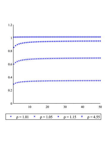
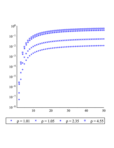
Figure 1: The left panel shows the ratio of our bound (4.19) to the bound (4.20) for the Legendre coefficients. The right panel shows the ratio of our bound (4.12) to the bound (4.21) for $\lambda=\frac{7}{2}$. Here $n$ ranges from $1$ to $50$.

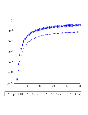
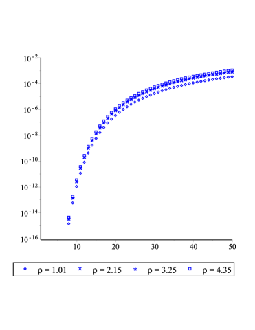
Figure 2: The ratio of our bound (4.12) to the bound (4.21) for $\lambda=\frac{11}{2}$ (left) and $\lambda=\frac{19}{2}$ (right). Here $n$ ranges from $1$ to $50$.

Remark 4.7.

For the function $Q_{n}^{(\lambda)}(z)$ which is defined in (3.4), we use the proof of Theorem 4.1, so that

$$\max_{z\in\mathcal{E}_{\rho}}|Q_{n}^{(\lambda)}(z)|=\left\{\begin{array}[]{ccc}{\displaystyle\frac{c_{n,\lambda}h_{n}^{(\lambda)}}{\rho^{n+1}}{}_{2}\mathrm{F}_{1}\left[\begin{matrix}n+1,&1-\lambda;\\ n+\lambda+1;&\end{matrix}\frac{1}{\rho^{2}}\right]},&\mbox{$\textstyle-\frac{1}{2}<\lambda\leq 1$ and $\lambda\neq 0$},\\[15.0pt] {\displaystyle\frac{c_{n,\lambda}h_{n}^{(\lambda)}}{\rho^{n+1}}{}_{2}\mathrm{F}_{1}\left[\begin{matrix}n+1,&1-\lambda;\\ n+\lambda+1;&\end{matrix}-\frac{1}{\rho^{2}}\right]},&\mbox{$\lambda>1$.}\end{array}\right.$$ (4.24)

For the former case, the maximum value can be attained at $z=\pm\frac{1}{2}(\rho+\rho^{-1})$. For the latter, the maximum value can be attained at $z=\pm\frac{i}{2}(\rho-\rho^{-1})$. We remark that (4.24) is very useful in establishing some uniform and explicit bounds for $Q_{n}^{(\lambda)}(z)$ or rigorous bounds for Gauss-Gegenbauer quadrature (see, for example, [12, 23, 33]). For example, when $\lambda=\frac{1}{2}$, $Q_{n}^{(\frac{1}{2})}(z)$ is exactly the Legendre function of the second kind. As is well-known, $Q_{n}^{(\frac{1}{2})}(x)$ is strictly monotonically decreasing on $(1,\infty)$. Therefore, for $x>1+\delta$ and $\delta>0$, by setting $\frac{1}{2}(\rho+\rho^{-1})=1+\delta$ and using Lemma 4.2 and (4.1), we have

$$|Q_{n}^{(\frac{1}{2})}(x)|<Q_{n}^{(\frac{1}{2})}(1+\delta)=\sqrt{\pi}\frac{\Gamma(n+1)}{\Gamma(n+\frac{3}{2})}{}_{2}\mathrm{F}_{1}\left[\begin{matrix}n+1,&\frac{1}{2};\\ n+\frac{3}{2};&\end{matrix}\frac{1}{\hat{\delta}^{2}}\right]\frac{1}{\hat{\delta}^{n+1}}\leq\frac{\sqrt{\pi}\Upsilon_{n}^{1,\frac{3}{2}}}{\hat{\delta}^{n}\sqrt{n(\hat{\delta}^{2}-1)}},$$ (4.25)

where $\hat{\delta}=1+\delta+\sqrt{(1+\delta)^{2}-1}$. In a very recent paper of Lederman and Rokhlin [23, Lemma 3.1], the authors provided the following bound for $Q_{n}^{(\frac{1}{2})}(x)$,

$$|Q_{n}^{(\frac{1}{2})}(x)|<\left(\log\left(2\frac{1+\tilde{\delta}}{\tilde{\delta}}\right)+1\right)\left(\frac{1}{1+\tilde{\delta}}\right)^{n+1},$$ (4.26)

where $\tilde{\delta}=\sqrt{(1+\delta)^{2}-1}$. Figure 3 illustrates the comparison of the above two bounds. Clearly, we can see that our bound (4.25) is much sharper, especially when $n$ is large.

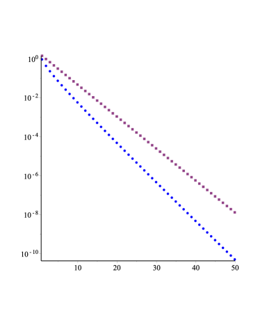
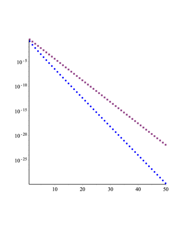
Figure 3: Comparison of our bound (4.25) (dots) with the bound (4.26) (boxes) for $\delta=0.1$ (left) and $\delta=1$ (right). Here $n$ ranges from $1$ to $50$.

4.2 Error bounds for truncated Gegenbauer expansion

Having established bounds for the Gegenbauer coefficients, we can immediately derive error bounds for the truncated Gegenbauer expansion. Let

$$f_{N}(x)=\sum_{n=0}^{N-1}a_{n}^{\lambda}C_{n}^{(\lambda)}(x).$$

We now give the first main result of this section.

Theorem 4.8.

Suppose that $f$ is analytic inside and on the Bernstein ellipse $\mathcal{E}_{\rho}$ with $\rho>1$. When $0<\lambda\leq 1$, the error of the truncated Gegenbauer expansion can be bounded by

$$\left|f(x)-f_{N}(x)\right|\leq\frac{ML(\mathcal{E}_{\rho})\Gamma(\lambda)}{\pi\Gamma(2\lambda)}\sum_{n=N}^{\infty}\frac{\Gamma(n+2\lambda)}{\Gamma(n+\lambda)\rho^{n+1}}{}_{2}\mathrm{F}_{1}\left[\begin{matrix}n+1,~{}1-\lambda;&\\ n+\lambda+1;&\end{matrix}\frac{1}{\rho^{2}}\right],$$ (4.27)

where $M$ and $L(\mathcal{E}_{\rho})$ are defined as in Theorem 4.1. In particular, when $\lambda=1$, the above bound can be given explicitly by

$$|f(x)-f_{N}(x)|\leq\frac{ML(\mathcal{E}_{\rho})}{\pi\rho^{N}}\left(\frac{N(\rho-1)+\rho}{(\rho-1)^{2}}\right).$$ (4.28)

When $\lambda>1$, the error of the truncated Gegenbauer series can be bounded by

$$\left|f(x)-f_{N}(x)\right|\leq\frac{ML(\mathcal{E}_{\rho})\Gamma(\lambda)}{\pi\Gamma(2\lambda)}\sum_{n=N}^{\infty}\frac{\Gamma(n+2\lambda)}{\Gamma(n+\lambda)\rho^{n+1}}{}_{2}\mathrm{F}_{1}\left[\begin{matrix}n+1,~{}1-\lambda;&\\ n+\lambda+1;&\end{matrix}-\frac{1}{\rho^{2}}\right].$$ (4.29)

Proof.

Using (2.3) we have

$$\left|f(x)-f_{N}(x)\right| =\left|\sum_{n=N}^{\infty}a_{n}^{\lambda}C_{n}^{(\lambda)}(x)\right|\leq\sum_{n=N}^{\infty}\left|a_{n}^{\lambda}\right|C_{n}^{(\lambda)}(1).$$ (4.30)

When $0<\lambda\leq 1$, by applying (1.1) and (4.1), one finds

$$\left|f(x)-f_{N}(x)\right| \leq\sum_{n=N}^{\infty}\frac{c_{n,\lambda}ML(\mathcal{E}_{\rho})}{\pi\rho^{n+1}}{}_{2}\mathrm{F}_{1}\left[\begin{matrix}n+1,~{}1-\lambda;&\\ n+\lambda+1;&\end{matrix}\frac{1}{\rho^{2}}\right]C_{n}^{(\lambda)}(1)$$

$$=\frac{ML(\mathcal{E}_{\rho})\Gamma(\lambda)}{\pi\Gamma(2\lambda)}\sum_{n=N}^{\infty}\frac{\Gamma(n+2\lambda)}{\Gamma(n+\lambda)\rho^{n+1}}{}_{2}\mathrm{F}_{1}\left[\begin{matrix}n+1,~{}1-\lambda;&\\ n+\lambda+1;&\end{matrix}\frac{1}{\rho^{2}}\right].$$

This proves (4.27). When $\lambda=1$, note that the Gauss hypergeometric function on the right hand side of the last equation is reduced to one and the above inequality can be further simplified as

$$\left|f(x)-f_{N}(x)\right| \leq\frac{ML(\mathcal{E}_{\rho})}{\pi}\sum_{n=N}^{\infty}\frac{n+1}{\rho^{n+1}}$$

$$=\frac{ML(\mathcal{E}_{\rho})}{\pi\rho^{N}}\left(\frac{N(\rho-1)+\rho}{(\rho-1)^{2}}\right).$$

This proves (4.28). Similarly, the case $\lambda>1$ can be proved with the use of (4.2) and (4.30). This completes the proof.

∎

The bound for the case $\lambda>1$ is very useful for analyzing the convergence of the diagonal Gegenbauer approximation (see, e.g., [4]). In what follows, we consider to establish a new upper bound which is simpler but surely less sharp than (4.29).

Theorem 4.9.

Under the same assumptions of Theorem 4.8. If $\lambda>1$ and $\rho>\frac{(N+2\lambda)(N+\lambda+1)}{(N+\lambda)(N+1)}$, then

$$\left|f(x)-f_{N}(x)\right|\leq\frac{\Gamma(\lambda)\Gamma(N+2\lambda)}{\Gamma(2\lambda)\Gamma(N+\lambda)}\left(1+\frac{1}{\rho^{2}}\right)^{\lambda-1}\frac{C}{\rho^{N}}.$$ (4.31)

where $C$ is defined by

$$C=\frac{ML(\mathcal{E}_{\rho})}{\pi}\left(\frac{(N+\lambda)(N+1)}{\rho(N+\lambda)(N+1)-(N+2\lambda)(N+\lambda+1)}\right).$$

Proof.

Define

$$H(n)=\frac{\Gamma(n+2\lambda)}{\Gamma(n+\lambda)\rho^{n+1}}{}_{2}\mathrm{F}_{1}\left[\begin{matrix}n+1,~{}1-\lambda;&\\ n+\lambda+1;&\end{matrix}-\frac{1}{\rho^{2}}\right].$$ (4.32)

Then, we have for $n\geq N$ that

$$\frac{H(n+1)}{H(n)}=\frac{n+2\lambda}{\rho(n+\lambda)}\frac{{}_{2}\mathrm{F}_{1}\left[\begin{matrix}n+2,~{}1-\lambda;&\\ n+\lambda+2;&\end{matrix}-\frac{1}{\rho^{2}}\right]}{{}_{2}\mathrm{F}_{1}\left[\begin{matrix}n+1,~{}1-\lambda;&\\ n+\lambda+1;&\end{matrix}-\frac{1}{\rho^{2}}\right]}.$$

Applying (4.4) to the ratio of Gauss hypergeometric functions yields

$$\frac{{}_{2}\mathrm{F}_{1}\left[\begin{matrix}n+2,~{}1-\lambda;&\\ n+\lambda+2;&\end{matrix}-\frac{1}{\rho^{2}}\right]}{{}_{2}\mathrm{F}_{1}\left[\begin{matrix}n+1,~{}1-\lambda;&\\ n+\lambda+1;&\end{matrix}-\frac{1}{\rho^{2}}\right]} =\frac{n+\lambda+1}{n+1}\frac{\int_{0}^{1}t^{n+1}(1-t)^{1-\lambda}(1+\frac{t}{\rho^{2}})^{\lambda-1}dt}{\int_{0}^{1}t^{n}(1-t)^{1-\lambda}(1+\frac{t}{\rho^{2}})^{\lambda-1}dt}\leq\frac{n+\lambda+1}{n+1}.$$

Therefore,

$$\frac{H(n+1)}{H(n)}\leq\frac{(n+2\lambda)(n+\lambda+1)}{\rho(n+\lambda)(n+1)}\leq\frac{(N+2\lambda)(N+\lambda+1)}{\rho(N+\lambda)(N+1)}.$$

Owing to the assumption on $\rho$, we see that the last bound is less than one. Combining this with (4.29) gives

$$|f(x)-f_{N}(x)| \leq\frac{ML(\mathcal{E}_{\rho})\Gamma(\lambda)}{\pi\Gamma(2\lambda)}\sum_{n=N}^{\infty}H(n)$$

$$\leq\frac{ML(\mathcal{E}_{\rho})\Gamma(\lambda)}{\pi\Gamma(2\lambda)}H(N)\sum_{m=0}^{\infty}\left(\frac{(N+2\lambda)(N+\lambda+1)}{\rho(N+\lambda)(N+1)}\right)^{m}$$

$$=\frac{ML(\mathcal{E}_{\rho})\Gamma(\lambda)}{\pi\Gamma(2\lambda)}\frac{H(N)\rho(N+\lambda)(N+1)}{\rho(N+\lambda)(N+1)-(N+2\lambda)(N+\lambda+1)}.$$

Combining this with (4.1) gives the desired result. This completes the proof. ∎

To overcome the Gibbs phenomenon, a Gegenbauer reconstruction method was developed in [13, 14, 15, 16, 17] and this method required to analyze the convergence of the diagonal Gegenbauer approximation, i.e., $\lambda$ depends linearly on $N$. We also refer the reader to [4] for further discussion. In this case, our bound (4.31) provides a rigorous and computable bound.

Corollary 4.10.

If $\lambda=\gamma N>1$ and $\gamma$ is a positive constant and $\rho>\frac{(1+2\gamma)((1+\gamma)N+1)}{(1+\gamma)(N+1)}$, then the error of the truncated Gegenbauer series can be bounded by

$$|f(x)-f_{N}(x)|\leq\frac{\Gamma(\gamma N)\Gamma((1+2\gamma)N)}{\Gamma(2\gamma N)\Gamma((1+\gamma)N)}\left(1+\frac{1}{\rho^{2}}\right)^{\gamma N-1}\frac{\tilde{C}}{\rho^{N}},$$ (4.33)

where

$$\tilde{C}=\frac{ML(\mathcal{E}_{\rho})}{\pi}\left(\frac{(1+\gamma)(N+1)}{\rho(1+\gamma)(N+1)-(1+2\gamma)((1+\gamma)N+1)}\right).$$

Proof.

If follows directly from Theorem 4.9 by setting $\lambda=\gamma N$. ∎

Example 4.11.

We illustrate the error bound (4.33) for the function $f(x)=\frac{1}{x-2}$. It is easy to check that this function is analytic inside the ellipse $\mathcal{E}_{\rho}$ with $1<\rho<2+\sqrt{3}\approx 3.732$ and

$$\max_{z\in\mathcal{E}_{\rho}}|f(z)|\leq M=\frac{2\rho}{(2+\sqrt{3}-\rho)(\rho-(2-\sqrt{3}))}.$$

We compare our bound (4.33) with the maximum error of the truncated Gegenbauer series

$$\max_{x\in[-1,1]}|f(x)-f_{N}(x)|$$

which is measured at $1000$ equispaced points in $[-1,1]$. In our computations, we choose $\rho=3.6$ and the perimeter of the ellipse is evaluated by the following formula [25, Eqn. (19.9.9)]

$$L(\mathcal{E}_{\rho})=\frac{4}{\epsilon}E(\epsilon),$$ (4.34)

where $\epsilon=\frac{2}{\rho+\rho^{-1}}$ and $E(z)$ is the complete ellipse integral of the second kind, although we remark that simple approximation formulas are also available (see, for example, [25, Eqn. (19.9.10)]). We test two values $\gamma=0.25$ and $\gamma=0.125$ and it is easy to check that these values of $\rho$ and $\gamma$ satisfy the assumptions of Corollary 4.10 when $N\geq 8$. All computations were performed using Maple with $100$ digits arithmetic. Numerical results are presented in Figure 4, which show that our bound is tight.

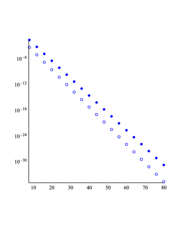
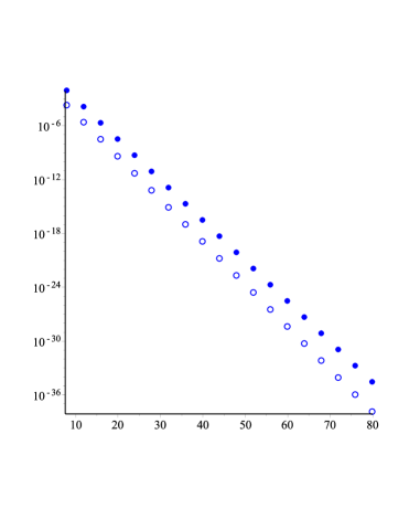
Figure 4: Comparison of our bound (4.33) (dots) with the maximum error (circles) for $\gamma=0.25$ (left) and $\gamma=0.125$ (right). Here $N$ ranges from $8$ to $80$.

Remark 4.12.

It was demonstrated in [4] that the singularities of $f(x)$ in the complex plane can ruin the convergence of the diagonal Gegenbauer approximation method unless the constant $\gamma$ is sufficiently small. This means that, to ensure the convergence of the diagonal Gegenbauer approximation method, there should be a lower bound on $\rho$ for each $\gamma$. The condition of $\rho$ in Corollary 4.10 provides a lower bound.

Remark 4.13.

For each fixed $\gamma$, the error bound (4.33) can be further optimized as a function of $\rho$.

5 A comparison of Legendre and Chebyshev coefficients

The most commonly used cases of Gegenbauer expansion are the Chebyshev and Legendre expansions which, up to normalization, correspond to the special cases $\lambda=0$ and $\lambda=\frac{1}{2}$, respectively. More specifically, the Legendre expansion is defined in (4.18) and the Chebyshev expansion of the first kind is defined by

$$f(x)=\sum_{n=0}^{\infty}{{}^{\prime}}a_{n}^{C}T_{n}(x),\quad a_{n}^{C}=\frac{2}{\pi}\int_{-1}^{1}\frac{f(x)T_{n}(x)}{\sqrt{1-x^{2}}}dx,$$ (5.1)

where the prime indicates that the first term of the sum is halved.

For both expansions, one particularly interesting question is the comparison of the decay rates of the Chebyshev and Legendre coefficients (see [6, 11, 22, 31]). For few decades, a myth on this issue is the “Lanczos-Fox-Parker” proposition which states that the Chebyshev coefficient $a_{n}^{C}$ decays approximately $\sqrt{n\pi}/2$ faster than the Legendre coefficient $a_{n}^{L}$ for large $n$. This proposition was first advocated by Lanczos in [22] and later by Fox and Parker in their monograph [11, p. 17]. The original deviation of this proposition was based on the use of Rodrigues’ formula of orthogonal polynomials and repeated integration by parts, which is not rigorous enough (see [24, p. 130]). Recently, Boyd and Petschek in [6] considered this issue and showed that the “Lanczos-Fox-Parker” proposition is not true for the following concrete examples

$$f(x)=\left\{\begin{array}[]{ccc}{\displaystyle\exp(rT_{m}(x))},&\mbox{$\textstyle r>0$ and $m$ is a large integer},\\[6.0pt] {\displaystyle\frac{1}{r-x}},&\mbox{$r>1$},\\[12.0pt] {\displaystyle(1-x)^{\phi}},&\mbox{$\phi>0$ is not an integer.}\end{array}\right.$$

Even these counterexamples were given, however, a precise result on the comparison of Legendre and Chebyshev coefficients is still nontrivial. In this section, inspired by these exceptions, we analyze this issue based on the contour integral expression of Gegenbauer coefficients. To this aim, we define the ratio of the $n$th Legendre coefficient to the $n$th Chebyshev coefficient as

$$\gamma_{n}=\frac{a_{n}^{L}}{a_{n}^{C}},\quad a_{n}^{C}\neq 0,\quad n\geq 0.$$ (5.2)

We shall discuss the asymptotic behaviour of $\gamma_{n}$.

Now we give the relation between the Gegenbauer coefficients and the Chebyshev and Legendre coefficients which will be used in our analysis.

Lemma 5.1.

Suppose that $a_{n}^{L}$, $a_{n}^{C}$ and $a_{n}^{\lambda}$ denote the Legendre, Chebyshev and Gegenbauer coefficients of the the same function $f(x)$, which are defined by (4.18), (5.1), and (1.5), respectively. Then $a_{n}^{L}=a_{n}^{\frac{1}{2}}$ for each $n\geq 0$, and

$$a_{n}^{C}=\frac{2}{n}\lim_{\lambda\rightarrow 0^{+}}\lambda a_{n}^{\lambda},\quad n\geq 1,$$

and $a_{0}^{C}=2\lim_{\lambda\rightarrow 0^{+}}a_{0}^{\lambda}$.

Proof.

The Legendre case follows from (2.4). As for the Chebyshev case, it follows directly from (2.5) for $n\geq 1$ and the fact that $C_{0}^{(0)}(x)=1$ for $n=0$. ∎

For simplicity of presentation, we assume that $f(z)$ has a single singularity such as a pole or branch point at $z=z_{0}$ in the complex plane, although it is not difficult to extend our results to the case that $f(z)$ has finite numbers of singularities. We distinguish three cases $z_{0}\in\mathbb{C}\setminus[-1,1]$, $z_{0}=\pm 1$ and $z_{0}\in(-1,1)$.

5.1 The case $z_{0}\in\mathbb{C}\setminus[-1,1]$

Before embarking on our analysis, we first introduce some helpful lemmas.

Lemma 5.2.

We have

$$c_{n,\frac{1}{2}}=\sqrt{n\pi}\left(1+\frac{1}{8n}+\mathcal{O}(n^{-2})\right),\quad n\rightarrow\infty.$$ (5.3)

Proof.

This is a direct consequence of Remark 3.5. ∎

Lemma 5.3.

For fixed $x\neq 1$, we have

$${}_{2}\mathrm{F}_{1}\left[\begin{matrix}a+\lambda,~{}b;&\\ c+\lambda;&\end{matrix}x\right]=(1-x)^{-b}\left[1+\frac{b(c-a)}{c+\lambda}\left(\frac{x}{1-x}\right)+\mathcal{O}(\lambda^{-2})\right],$$ (5.4)

as $\lambda\rightarrow\infty$.

Proof.

See [28]. ∎

Consider the following model function

$$f(x)=\frac{1}{x-z_{0}},\quad z_{0}\in\mathbb{C}\setminus[-1,1],$$ (5.5)

which has a simple pole at $x=z_{0}$. This function provides valuable insights for the asymptotic behaviour of $\gamma_{n}$ for large $n$. Our main result is stated in the following theorem.

Theorem 5.4.

For the function (5.5), we have

$$\gamma_{n}=g(z_{0})\sqrt{n\pi}+\mathcal{O}(n^{-\frac{1}{2}}),\quad n\rightarrow\infty,$$ (5.6)

where $g(z)$ is defined by

$$g(z)=\sqrt{\frac{z^{2}-1}{(z\pm\sqrt{z^{2}-1})^{2}-1}},$$ (5.7)

and the sign is chosen such that $|z\pm\sqrt{z^{2}-1}|>1$ and $g(z)>0$ if $z>1$.

Proof.

If follows from (4.6) with $b=z_{0}$ that

$$a_{n}^{\lambda}=-\frac{2c_{n,\lambda}}{(z_{0}\pm\sqrt{z_{0}^{2}-1})^{n+1}}{}_{2}\mathrm{F}_{1}\left[\begin{matrix}n+1,~{}1-\lambda;&\\ n+\lambda+1;&\end{matrix}\frac{1}{(z_{0}\pm\sqrt{z_{0}^{2}-1})^{2}}\right],\quad n\geq 0.$$

By the Lemma 5.1,

$$a_{n}^{L}=-\frac{2c_{n,\frac{1}{2}}}{(z_{0}\pm\sqrt{z_{0}^{2}-1})^{n+1}}{}_{2}\mathrm{F}_{1}\left[\begin{matrix}n+1,~{}\frac{1}{2};&\\ n+\frac{3}{2};&\end{matrix}\frac{1}{(z_{0}\pm\sqrt{z_{0}^{2}-1})^{2}}\right],\quad n\geq 0,$$

and

$$a_{n}^{C}=-\frac{2}{\sqrt{z_{0}^{2}-1}(z_{0}\pm\sqrt{z_{0}^{2}-1})^{n}},\quad n\geq 0.$$

Now combining the above two equations, we see that

$$\gamma_{n}=\frac{c_{n,\frac{1}{2}}\sqrt{z_{0}^{2}-1}}{z_{0}\pm\sqrt{z_{0}^{2}-1}}{}_{2}\mathrm{F}_{1}\left[\begin{matrix}n+1,~{}\frac{1}{2};&\\ n+\frac{3}{2};&\end{matrix}\frac{1}{(z_{0}\pm\sqrt{z_{0}^{2}-1})^{2}}\right],\quad n\geq 0.$$ (5.8)

This together with Lemma 5.2 and Lemma 5.3 gives the desired result. ∎

Remark 5.5.

We remark that the result (5.6) still holds if $z_{0}$ is a singularity of algebraic or logarithmic type. The key point is that the Chebyshev and Legendre coefficients can be estimated accurately by evaluating their contour integral expressions at the singularity multiplied by some common factors. For example, when $f(x)=(b-x)^{\alpha}$ where $b>1$ and $\alpha>-1$ is not an integer. From [8], we have that

$$a_{n}^{C}=\frac{\xi(\alpha,b)}{\sqrt{b^{2}-1}(b+\sqrt{b^{2}-1})^{n}}\left(1+\mathcal{O}(n^{-1})\right),\quad n\rightarrow\infty,$$

where $\xi(\alpha,b)$ is defined by

$$\xi(\alpha,b)=-\frac{2\sin(\alpha\pi)(b^{2}-1)^{\frac{\alpha+1}{2}}\Gamma(\alpha+1)}{\pi n^{\alpha+1}}.$$

Adapting the similar arguments and Lemma 5.2 and Lemma 5.3 gives

$$a_{n}^{L}=\frac{\xi(\alpha,b)}{\sqrt{b^{2}-1}(b+\sqrt{b^{2}-1})^{n}}\left(\sqrt{n\pi}g(b)+\mathcal{O}(n^{-\frac{1}{2}})\right),\quad n\rightarrow\infty,$$

where $g(b)$ is defined as in (5.7). Combining the above two estimates, it is easy to check that (5.6) still holds; see Figure 6 for numerical illustrations.

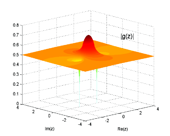
Figure 5: Absolute value of the function $g(z)$ in the complex plane.

Remark 5.6.

It is easily seen that $g(z)=0$ when $z=\pm 1$; otherwise, $g(z)\neq 0$. This leads us to consider that the asymptotic behaviour of $\gamma_{n}$ will be greatly different if $z_{0}$ is an endpoint singularity. Indeed, we shall show the ratio $\gamma_{n}$ tends to some constants as $n$ grows in this case. Moreover, when $g(z_{0})\neq 0$, we can deduce that the Chebyshev coefficient $a_{n}^{C}$ decays approximately $g(z_{0})\sqrt{n\pi}$ faster than the Legendre coefficient $a_{n}^{L}$.

Remark 5.7.

It is not difficult to verify that $\lim_{|z|\rightarrow\infty}g(z)=\frac{1}{2}$ and $g(z)\neq\frac{1}{2}$ for any finite $|z|$, which implies that the “Lanczos-Fox-Parker” proposition is always false for functions that have a singularity in the complex plane. Figure 5 illustrates the absolute value of $g(z)$ in the complex plane. We can see that $|g(z)|$ converges to $\frac{1}{2}$ as $|z|\rightarrow\infty$. Meanwhile, we also observe that $|g(z)|$ attains its maximum value at $z=0$ and $|g(0)|=\frac{1}{\sqrt{2}}$, which implies that the fastest possible rate of growth of $\gamma_{n}$ will be close to $\sqrt{\frac{n\pi}{2}}$ as $n$ grows.

Remark 5.8.

When the pole $z_{0}$ is real, we have

$$g(z_{0})=\left\{\begin{array}[]{ccc}{\displaystyle\sqrt{\frac{z_{0}^{2}-1}{(z_{0}+\sqrt{z_{0}^{2}-1})^{2}-1}}},&\mbox{$z_{0}>1$, }\\[14.0pt] {\displaystyle\sqrt{\frac{z_{0}^{2}-1}{(z_{0}-\sqrt{z_{0}^{2}-1})^{2}-1}}},&\mbox{$z_{0}<-1$}.\end{array}\right.$$ (5.11)

It is easy to verify that $g(z_{0})$ is monotonically decreasing on the interval $(-\infty,-1)$ and is monotonically increasing on the interval $(1,\infty)$ and $\lim_{z_{0}\rightarrow\pm 1}g(z_{0})=0$ and $\lim_{z_{0}\rightarrow\pm\infty}g(z_{0})=\frac{1}{2}$. If the pole lies on the imaginary axis, e.g., $z_{0}=ib$ where $b$ is a real and nonzero constant, then

$$g(z_{0})=g(ib)=\left\{\begin{array}[]{ccc}{\displaystyle\sqrt{\frac{b^{2}+1}{(b+\sqrt{b^{2}+1})^{2}+1}}},&\mbox{$b>0$, }\\[12.0pt] {\displaystyle\sqrt{\frac{b^{2}+1}{(b-\sqrt{b^{2}+1})^{2}+1}}},&\mbox{$b<0$}.\end{array}\right.$$ (5.14)

It can be seen that $g(z_{0})$ is monotonically increasing when $b\in(-\infty,0)$ and is monotonically decreasing function when $b\in(0,\infty)$ and

$$\lim_{b\rightarrow\pm 0}g(ib)=\frac{1}{\sqrt{2}},\quad\lim_{b\rightarrow\pm\infty}g(ib)=\frac{1}{2}.$$

These properties can be confirmed from Figure 5.

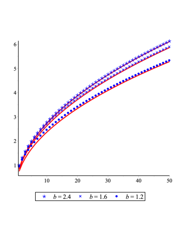
Figure 6: The exact values of ratio $\gamma_{n}$ (dots, asterisks and crosses) and the predicted values $g(b)\sqrt{n\pi}$ (lines) for $f(x)=\log(b-x)$ (left) and $f(x)=(b-x)^{\frac{2}{3}}$ (right). Here $n$ ranges from $1$ to $50$.

Example 5.9.

For model functions such as

$$f(x)=\log(b\pm x),~{}(b\pm x)^{\alpha},$$

where $b>1$ and $\alpha$ is not a nonegative integer. It follows from Theorem 5.4 and Remark 5.5 that

$$\gamma_{n}=g(b)\sqrt{n\pi}+\mathcal{O}(n^{-\frac{1}{2}}),\quad n\rightarrow\infty,$$

where $g(b)$ is given by (5.7), e.g.,

$$g(b)=\sqrt{\frac{b^{2}-1}{(b+\sqrt{b^{2}-1})^{2}-1}}.$$ (5.15)

In Figure 6, we illustrate the exact values of $\gamma_{n}$ and the predicted values $g(b)\sqrt{n\pi}$ for two functions $f(x)=\log(b-x)$ and $f(x)=(b-x)^{\frac{2}{3}}$, where $g(b)$ is defined by (5.15). For each function, we show numerical results for three values of $b$. As expected, the asymptotic behaviour of $\gamma_{n}$ is in excellent agreement with our predicted values.

5.2 The case $z_{0}=\pm 1$

In this subsection we consider the case that $z_{0}$ is an endpoint singularity. Boyd and Petschek in [6] considered the special case $f(x)=(1-x)^{\alpha}$ where $\alpha>0$ is not an integer and showed that the decay rate of the Chebyshev coefficient $a_{n}^{C}$ is the same as that of the Legendre coefficient $a_{n}^{L}$. In what follows, we consider the asymptotic behaviour of $\gamma_{n}$ for the model functions $f(x)=\log(1\pm x)$ and $f(x)=(1\pm x)^{\alpha}$ where $\mathrm{Re}\,(\alpha)>-\frac{1}{2}$ is not an integer. We present delicate results on the asymptotic behaviour of $\gamma_{n}$.

Theorem 5.10.

For the functions $f(x)=(1\pm x)^{\alpha}$ where $\mathrm{Re}\,(\alpha)>-\frac{1}{2}$ is not an integer, we have

$$\gamma_{n}=\frac{\Gamma(\alpha+1)}{\Gamma(\alpha+\frac{1}{2})}\sqrt{\pi}+\mathcal{O}(n^{-1}),\quad n\rightarrow\infty.$$ (5.16)

For the functions $f(x)=\log(1\pm x)$, we have

$$\gamma_{n}=1+\mathcal{O}(n^{-1}),\quad n\rightarrow\infty.$$ (5.17)

Proof.

We consider the case $f(x)=(1-x)^{\alpha}$. Since the Legendre and Chebyshev coefficients correspond to the special case $\lambda=\frac{1}{2}$ and $\lambda=0$, respectively, we have from Lemma 5.1 and Lemma A.1 that

$$a_{n}^{L}=(-1)^{n}\frac{2^{\alpha+1}\Gamma(\alpha+1)^{2}(n+\frac{1}{2})}{\Gamma(\alpha-n+1)\Gamma(\alpha+n+2)},$$

where $\mathrm{Re}\,(\alpha)>-1$, and

$$a_{n}^{C}=(-1)^{n}\frac{2^{\alpha+1}\Gamma(\alpha+\frac{1}{2})\Gamma(\alpha+1)}{\sqrt{\pi}\Gamma(\alpha-n+1)\Gamma(\alpha+n+1)},$$

where $\mathrm{Re}\,(\alpha)>-\frac{1}{2}$. Thus, when $\mathrm{Re}\,(\alpha)>-\frac{1}{2}$, combining the above two equations, we get

$$\gamma_{n}=\left(n+\frac{1}{2}\right)\frac{\Gamma(n+\alpha+1)}{\Gamma(n+\alpha+2)}\frac{\Gamma(\alpha+1)}{\Gamma(\alpha+\frac{1}{2})}\sqrt{\pi},~{}~{}n\geq 0.$$

By using (3.14), the result (5.16) follows. For the case $f(x)=\log(1-x)$, using Lemma 5.1 and Lemma A.2 we see that

$$a_{n}^{L}=-\frac{2n+1}{n(n+1)},\quad a_{n}^{C}=-\frac{2}{n},$$

for each $n\geq 1$. Hence the result (5.17) follows. The other cases $f(x)=(1+x)^{\alpha},~{}\log(1+x)$ can be proved similarly and we omit the details. This proves Theorem 5.10. ∎

Remark 5.11.

For functions of the form $f(x)=(1\pm x)^{\alpha}$, where $\mathrm{Re}\,(\alpha)>-\frac{1}{2}$ is not an integer, Theorem 5.10 implies that the Chebyshev coefficient $a_{n}^{C}$ decays $\frac{\Gamma(\alpha+1)}{\Gamma(\alpha+\frac{1}{2})}\sqrt{\pi}$ faster than its Legendre counterpart $a_{n}^{L}$. For functions of the form $f(x)=\log(1\pm x)$, however, both coefficients are almost the same for large $n$.

Remark 5.12.

For more general functions such as $f(x)=(1\pm x)^{\alpha}h(x)$ and $f(x)=\log(1\pm x)h(x)$ where $\mathrm{Re}\,(\alpha)>-\frac{1}{2}$ is not an integer and $h(x)$ is analytic in a neighborhood of the interval $[-1,1]$, note that the main contributions to the Chebyshev and Legendre coefficients come from the endpoint singularity, it is not difficult to verify that the results of Theorem 5.10 still hold.

5.3 The case $z_{0}\in(-1,1)$

When the singularity $z_{0}\in(-1,1)$, we are not able to derive the asymptotic behaviour of their Chebyshev and Legendre coefficients, since in this case $f(z)$ is not analytic and their contour integral expressions can not be used.

The special case $f(x)=|x|$ has been analyzed in [6] and it was shown that $\gamma_{n}/\sqrt{n\pi}\sim\frac{1}{\sqrt{2}}$ as $n\rightarrow\infty$. However, the situation becomes much more complicated when $z_{0}\neq 0$. As an illustrative example, we show the behaviour of $\gamma_{n}/\sqrt{n\pi}$ for $f(x)=\log|x-\frac{1}{4}|$ and $f(x)=|x-\frac{1}{4}|^{\frac{1}{2}}$ in Figure 7. It is clear to see that $\gamma_{n}/\sqrt{n\pi}$ oscillates around some finite values. On the other hand, we can also see that $\gamma_{n}/\sqrt{n\pi}=\mathcal{O}(1)$, which implies that $a_{n}^{C}$ decays $\mathcal{O}(\sqrt{n})$ faster than $a_{n}^{L}$. However, a precise result on the asymptotic behaviour of $\gamma_{n}$ is still open.

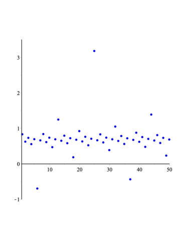
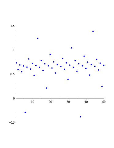
Figure 7: The values of $\frac{\gamma_{n}}{\sqrt{n\pi}}$ for $f(x)=\log|x-\frac{1}{4}|$ (left) and $f(x)=|x-\frac{1}{4}|^{\frac{1}{2}}$ (right). Here $n$ ranges from $1$ to $50$.

6 Concluding remarks

Gegenbauer expansion is an important tool in the resolution of Gibbs phenomenon and the numerical solution of differential equations. In this work, we have proposed a simple derivation of the contour integral expression of the coefficients in the Gegenbauer series expansion. We have derived optimal and explicit estimates for the Gegenbauer coefficients and these estimates are sharper than the existing ones. We further apply these optimal estimates to establish some rigorous and computable bounds for the truncated Gegenbauer series in the uniform norm. Additionally, we also consider the comparison of the decay rates of the Legendre and Chebyshev coefficients. Delicate results on the asymptotic behaviour of the ratio of the Legendre coefficient $a_{n}^{L}$ to the Chebyshev coefficient $a_{n}^{C}$ are presented.

We point out that our results can be easily extended to the comparison of spectral methods based on Chebyshev and Legendre expansions. It is well known that the maximum error of the truncated Chebyshev expansion can be estimated approximately by the absolute value of the first neglected term if the Chebyshev coefficients decay rapidly; see [9]. This implies the comparison of spectral methods using Chebyshev and Lgendre expansions can be approximately transformed into the comparison of the corresponding Legendre and Chebyshev coefficients. For example, if the singularity of $f$ is outside the interval $[-1,1]$ which implies that the Legendre and Chebyshev coefficients decay exponentially, then we can deduce that the rate of convergence of the spectral method using Chebyshev expansion is $\mathcal{O}(\sqrt{n})$ faster than that of its Legendre counterpart, where $n$ is the number of terms in both expansions.

Appendix A Gegenbauer expansion coefficients of functions with endpoint singularities

We present explicit formulas of the Gegenbauer expansion coefficients for $f(x)=\log(1\pm x)$ and $f(x)=(1\pm x)^{\alpha}$ where $\mathrm{Re}\,(\alpha)>-\frac{1}{2}$ is not an integer.

Lemma A.1.

For the functions $f(x)=(1\pm x)^{\alpha}$ where $\mathrm{Re}\,(\alpha)>-\frac{1}{2}$ is not an integer. Then, for $\mathrm{Re}\,(\lambda)>-\frac{1}{2}$ and $\mathrm{Re}\,(\lambda+\alpha)>-\frac{1}{2}$,

$$a_{n}^{\lambda}=\mu_{n}\frac{2^{4\lambda+\alpha-1}\Gamma(\lambda)^{2}\Gamma(\alpha+\lambda+\frac{1}{2})\Gamma(\lambda+\frac{1}{2})\Gamma(\alpha+1)(n+\lambda)}{\pi\Gamma(2\lambda)\Gamma(\alpha-n+1)\Gamma(\alpha+2\lambda+n+1)},~{}~{}n\geq 0,$$ (A.1)

where $\mu_{n}=(-1)^{n}$ when $f(x)=(1-x)^{\alpha}$ and $\mu_{n}=1$ when $f(x)=(1+x)^{\alpha}$.

Proof.

We only consider the case $f(x)=(1-x)^{\alpha}$ since the argument in the case $f(x)=(1+x)^{\alpha}$ is similar. For each $n\geq 0$, using the definition of $a_{n}^{\lambda}$ we have

$$a_{n}^{\lambda}=\frac{1}{h_{n}^{(\lambda)}}\int_{-1}^{1}(1-x)^{\alpha+\lambda-\frac{1}{2}}(1+x)^{\lambda-\frac{1}{2}}C_{n}^{(\lambda)}(x)dx.$$

Using [18, Eqn. 7.311] gives (A.1). This completes the proof. ∎

Lemma A.2.

For the functions $f(x)=\log(1\pm x)$. For each $n\geq 1$, their Gegenbauer coefficients can be written explicitly by

$$a_{n}^{\lambda}=\mu_{n}\frac{4^{\lambda}\Gamma(\lambda)\Gamma\left(\lambda+\frac{1}{2}\right)}{\sqrt{\pi}}\frac{\Gamma(n+1)\Gamma(n+\lambda+1)}{n\Gamma(n+\lambda)\Gamma(n+1+2\lambda)},$$ (A.2)

where $\mu_{n}=-1$ when $f(x)=\log(1-x)$ and $\mu_{n}=(-1)^{n+1}$ when $f(x)=\log(1+x)$.

Proof.

We first consider the case $f(x)=\log(1-x)$. Following the ideas exposed in [8], the contour integral of the $a_{n}^{\lambda}$ can be deformed as an ellipse $\mathcal{E}_{R}$ in the positive direction and a small circle with center at $z=1$ in the negative direction. Meanwhile, these two contours are connected by two line segments which are parallel and above and below the real axis. Letting $R\rightarrow\infty$ and the radius of the circle tend to zero, we note that the integral along $\mathcal{E}_{R}$ vanishes for each $n\geq 1$ and the integral along the circle vanishes. Thus, combining the contributions to $a_{n}^{\lambda}$ from these two line segments we find

$$a_{n}^{\lambda} =-2c_{n,\lambda}\int_{1}^{\infty}\frac{1}{(t+\sqrt{t^{2}-1})^{n+1}}{}_{2}\mathrm{F}_{1}\left[\begin{matrix}n+1,&1-\lambda;\\ n+\lambda+1;&\end{matrix}\frac{1}{(t+\sqrt{t^{2}-1})^{2}}\right]dt.$$

Setting $t=\cosh\theta$ and using some elementary calculations gives (A.2). The case $f(x)=\log(1+x)$ can be handled similarly and we omit the details. This completes the proof. ∎

References

- [1] G. E. Andrews, R. Askey, and R. Roy. Special functions. Cambridge University Press, 2000.
- [2] K. Atkinson and W. Han. Spherical Harmonics and Approximations on the Unit Sphere: An Introduction. Lecture Notes in Math. 2044, Springer, 2012.
- [3] S. N. Bernstein. Sur l’ordre de la meilleure approximation des fonctions continues par les polynomes de degré donné. Mem. Cl. Sci. Acad. Roy. Belg., pages 1–103, 1912.
- [4] J. P. Boyd. Trouble with Gegenbauer reconstruction for defeating Gibbs’ phenomenon: Runge phenomenon in the diagonal limit of Gegenbauer polynomial approximations. Journal of Computational Physics, 204(1):253–264, 2005.
- [5] J. P. Boyd. Large-degree asymptotics and exponential asymptotics for Fourier, Chebyshev and Hermite coefficients and Fourier transforms. Journal of Engineering Mathematics, 63(2-4):355–399, 2009.
- [6] J. P. Boyd and R. Petschek. The relationships between Chebyshev, Legendre and Jacobi polynomials: The generic superiority of Chebyshev polynomials and three important exceptions. Journal of Scientific Computing, 59(1):1–27, 2014.
- [7] M. J. Cantero and A. Iserles. On rapid computation of expansions in ultraspherical polynomials. SIAM Journal on Numerical Analysis, 50(1):307–327, 2012.
- [8] D. Elliott. The evaluation and estimation of the coefficients in the Chebyshev series expansion of a function. Mathematics of Computation, 18(86):274–284, 1964.
- [9] D. Elliott. Truncation errors in two Chebyshev series approximations. Mathematics of Computation, 19(90):234–248, 1965.
- [10] D. Elliott and P. Tuan. Asymptotic estimates of Fourier coefficients. SIAM Journal on Mathematical Analysis, 5(1):1–10, 1974.
- [11] L. Fox and I. B. Parker. Chebyshev polynomials in numerical analysis. 1968.
- [12] W. Gautschi and R. S. Varga. Error bounds for Gaussian quadrature of analytic functions. SIAM Journal on Numerical Analysis, 20(6):1170–1186, 1983.
- [13] D. Gottlieb and C.-W. Shu. On the Gibbs phenomenon IV: Recovering exponential accuracy in a subinterval from a Gegenbauer partial sum of a piecewise analytic function. Mathematics of Computation, 64(211):1081–1095, 1995.
- [14] D. Gottlieb and C.-W. Shu. On the Gibbs phenomenon V: Recovering exponential accuracy from collocation point values of a piecewise analytic function. Numerische Mathematik, 71(4):511–526, 1995.
- [15] D. Gottlieb and C.-W. Shu. On the Gibbs phenomenon III: Recovering exponential accuracy in a sub-interval from a spectral partial sum of a pecewise analytic function. SIAM Journal on Numerical Analysis, 33(1):280–290, 1996.
- [16] D. Gottlieb and C.-W. Shu. On the Gibbs phenomenon and its resolution. SIAM Review, 39(4):644–668, 1997.
- [17] D. Gottlieb, C.-W. Shu, A. Solomonoff, and H. Vandeven. On the Gibbs phenomenon I: Recovering exponential accuracy from the Fourier partial sum of a nonperiodic analytic function. Journal of Computational and Applied Mathematics, 43(1):81–98, 1992.
- [18] I. S. Gradshteyn and I. M. Ryzhik. Table of Integrals, Series, and Products. Academic Press, 2007.
- [19] B.-Y. Guo. Gegenbauer approximation in certain Hilbert spaces and its applications to singular differential equations. SIAM Journal on Numerical Analysis, 37(2):621–645, 2000.
- [20] A. Iserles. A fast and simple algorithm for the computation of Legendre coefficients. Numerische Mathematik, 117(3):529–553, 2011.
- [21] G. J. O. Jameson. Inequalities for the perimeter of an ellipse. The Mathematical Gazette, 98(542):227–234, 2014.
- [22] C. Lanczos. Tables of Chebyshev polynomials and . Applied Mathematics Series, No. 9, United States Government Printing Office, 1952.
- [23] R. R. Lederman and V. Rokhlin. On the analytical and numerical properties of the truncated Laplace transform I. SIAM Journal on Numerical Analysis, 53(3):1214–1235, 2015.
- [24] J. C. Mason and D. C. Handscomb. Chebyshev polynomials. Chapman and Hall/CRC Press, Boca Raton, FL, 2003.
- [25] F. W. J. Olver, D. W. Lozier, R. F. Boisvert, and C. W. Clark. NIST Handbook of Mathematical Functions. Cambridge University Press, 2010.
- [26] S. Olver and A. Townsend. A fast and well-conditioned spectral method. SIAM Review, 55(3):462–489, 2013.
- [27] G. Szegő. Orthogonal polynomials, volume 23. American Mathematical Society, 1939.
- [28] N. M. Temme. Large parameter cases of the Gauss hypergeometric function. Journal of Computational and Applied Mathematics, 153(1):441–462, 2003.
- [29] L. N. Trefethen. Approximation theory and approximation practice. SIAM, 2013.
- [30] H.-Y. Wang and D. Huybrechs. Fast and accurate computation of Jacobi expansion coefficients of analytic functions. arXiv:1404.2463, 2014.
- [31] H.-Y. Wang and S.-H. Xiang. On the convergence rates of Legendre approximation. Mathematics of Computation, 81(278):861–877, 2012.
- [32] S.-H. Xiang. On error bounds for orthogonal polynomial expansions and Gauss-type quadrature. SIAM Journal on Numerical Analysis, 50(3):1240–1263, 2012.
- [33] X.-D. Zhao, L.-L. Wang, and Z.-Q. Xie. Sharp error bounds for Jacobi expansions and Gegenbauer–Gauss quadrature of analytic functions. SIAM Journal on Numerical Analysis, 51(3):1443–1469, 2013.