Realization of the Lepton Flavor Structure from Point Interactions

Abstract

We investigate a 5d gauge theory on $S^{1}$ with point interactions. The point interactions describe extra boundary conditions and provide three generations, the charged lepton mass hierarchy, the lepton flavor mixing and tiny degenerated neutrino masses after choosing suitable boundary conditions and parameters. The existence of the restriction in the flavor mixing, which appears from the configuration of the extra dimension, is one of the features of this model. Tiny Yukawa couplings for the neutrinos also appears without the see-saw mechanism nor symmetries in our model. The magnitude of CP violation in the leptons can be a prediction and is consistent with the current experimental data.

1 Introduction

The Standard Model (SM) has done well until today. However, it does not mean that there is no problem. Even though a SM-like Higgs was found, the problems relating to the Yukawa couplings are left. The generation problem is one of them. Both in the quark sector and the lepton sector, we have the structure of the three generations. Every generation has exactly the same quantum numbers except for their masses. There is only a phenomenological reason to introduce the three generations, which is for the CP phase Kobayashi:1973fv , but there is no theoretical reason to them. The mass hierarchy is another one. There exists a large mass hierarchy for the quarks and the charged leptons. In the SM, the Yukawa couplings are just parameters and there is no reason for producing a large mass hierarchy. Tininess in the neutrino masses is also another problem. From experimental data, it had been found that the differences in the squared neutrino masses are of order ${\cal O}(10^{-4}-10^{-3})$ eV. The origin of the tiny neutrino masses is still unknown. The flavor mixing structure of the quark sector and the lepton sector, which is controlled by the Cabbibo-Kobayashi-Maskawa (CKM) matrix and the Pontecorvo-Maki-Nakagawa-Sakata (PMNS) matrix in the SM, is also a mystery. Due to the improvement of experiments, every mixing angle is measured with the CP phase in the quark sector, however, it is still unknown what kind of dynamics controls these values. Not only the above problems but also many other problems remain in the SM.

A way to solve the above problems in the SM is to use extra dimensions. Especially, 5d gauge theories with point interactions is an attractive one for solving the generation problem and the mass hierarchy problem in the fermions with producing the realistic flavor mixing angle from the extra dimension Fujimoto:2012wv ; Fujimoto:2014fka . In the paper Fujimoto:2012wv , the generation problem and the mass hierarchy problem in the quark sector are discussed and are solved with the realistic flavor mixing and the CP phase. In the research Fujimoto:2014fka , it turns out that we can apply the same method to the lepton sector for solving the generation problem and the mass hierarchy problem in the charged leptons with producing tiny neutrino masses and the realistic flavor mixing. The point interaction is a generalized zero-width interaction, an example of which is a delta-function potential in 1d quantum mechanics (QM) Reed:1975uy ; Seva1986 ; Cheon:2000tq , and is a key ingredient to produce the degenerated zero-mode functions, which is nothing but generations. By using the point interactions, we can put extra boundary conditions (BC’s) for the fermions at that points as in the case of the delta-function potential in 1d QM. Because of this (extra) BC’s, we can produce triply-degenerated zero-mode functions, which is nothing but three generations, without breaking the 5d gauge invariance. Since each triply-degenerated mode function lives in a different part of the extra dimension with localization toward the (extra) boundary points, we can produce a large hierarchy for the masses of the fermions through the overlap integrals if we introduce a 5d gauge-singlet scalar, which possesses an extra-dimensional coordinate-dependent vacuum expectation value (VEV) due to the BC’s. The tiny degenerated neutrino masses are also realized in this model. The magnitude of the localization of the zero-mode functions is controlled by the bulk masses of the 5d fermions. To realize the tiny neutrino masses, we should produce the extremely tight localization with setting the values of the bulk masses large. Because of this tight localization, the effect of the gauge-single scalar VEV becomes small, so that a hierarchical mass structure does not appear in the neutrinos. A characteristic feature of this model is that the flavor mixing is restricted by the geometry of the extra dimension. Because of this fact, we cannot fill up all the elements of the mass matrix but only 6 we can. Thus it is non-trivial whether we can reproduce experimental values in the model though we have more parameters than the Standard Model. Furthermore, the magnitude of CP violation in the lepton sector can be a prediction in this model because we have only one source for the CP phase, which is nothing but a Higgs VEV Fujimoto:2013ki . In our model, the Higgs VEV has a extra-dimensional coordinate-dependent phase with containing a twist parameter, which appears to the BC’s for the Higgs. This extra-dimensional coordinate-dependent phase is the only source of the CP phase. When we treat the quark sector and the lepton sector at the same time, the twist parameter is used to fix the magnitude of CP violation in the quark sector so that the magnitude of CP violation in the lepton sector is automatically determined Fujimoto:2014fka .

2 Lepton flavor structure from point interactions

2.1 A model

Our model consists of the following action.

$$S=S_{{\rm lepton}}+S_{{\rm Higgs}}+S_{{\rm singlet}}+S_{{\rm Yukawa}}^{({\rm lepton})},$$ (1)

$$S_{{\rm lepton}}=\int d^{4}x\int^{L}_{0}dy\left[\overline{L}(x,y)\Bigl{(}i\Gamma^{N}D_{N}^{(L)}+M_{L}\Bigr{)}L(x,y)\right.$$

$$\left.\hskip 30.00005pt+\overline{{\cal N}}(x,y)\Bigl{(}i\Gamma^{N}{\partial_{N}}+M_{{\cal N}}\Bigr{)}{\cal N}(x,y)+\overline{E}(x,y)\Bigl{(}i\Gamma^{N}D_{N}^{(E)}+M_{E}\Bigr{)}E(x,y)\right],$$ (2)

$$S_{{\rm Higgs}}=\int d^{4}x\int^{L}_{0}dy\left[H^{\dagger}(x,y)\Bigl{(}D^{N}D_{N}+M^{2}\Bigr{)}H(x,y)-\frac{\lambda}{2}\Bigl{(}H^{\dagger}(x,y)H(x,y)\Bigr{)}^{2}\right],$$ (3)

$$S_{{\rm singlet}}=\int d^{4}x\int^{L}_{0}dy\left[\Phi^{\dagger}(x,y)\Bigl{(}\partial^{N}\partial_{N}-M_{\Phi}^{2}\Bigr{)}\Phi(x,y)-\frac{\lambda_{\Phi}}{2}\Bigl{(}\Phi^{\dagger}(x,y)\Phi(x,y)\Bigr{)}^{2}\right],$$ (4)

$$S_{{\rm Yukawa}}^{({\rm lepton})}=\int d^{4}x\int^{L}_{0}dy\left[\Phi\Bigl{(}-{\cal Y}^{({\cal N})}\overline{L}(i\sigma_{2}H^{\ast}){\cal N}-{\cal Y}^{(E)}\overline{L}HE\Bigr{)}+({\rm h.c.})\right]{,}$$ (5)

where we denote $L(x,y)$ as an $SU(2)_{W}$ doublet lepton, ${\cal N}(x,y)$ as an $SU(2)_{W}$ singlet neutrino, $E(x,y)$ as an $SU(2)_{W}$ singlet charged lepton, $H(x,y)$ as the Higgs doublet and $\Phi(x,y)$ as a gauge singlet scalar field, respectively. $M_{\Psi}\ (\Psi=L,{\cal N},E)$ in Eq. (2) denotes the bulk mass for the fermions, which is important to control the mass hierarchy in our model. We put the signs as

$$M_{L}<0,$$ (6)

$$M_{{\cal N}}>0,$$ (7)

$$M_{E}<0,$$ (8)

for our purpose. Here, we omit the action for the $SU(3)_{C}\times SU(2)_{W}\times U(1)_{Y}$ gauge fields for the simplicity.

Note that the discrete symmetry, $H\rightarrow-H$, $\Phi\rightarrow-\Phi$, is introduced to forbid the terms $\bar{L}(i\sigma_{2}H^{\ast}){\cal N}$, $\bar{L}HE$, $\Phi\bar{L}L$, $\Phi\bar{{\cal N}}{\cal N}$, $\Phi\bar{E}E$. We also simply ignore the term $(H^{\dagger}H)(\Phi^{\dagger}\Phi)$ in this model.

In the case of an extra dimension scenario, not only the action but also the BC’s are important. In our model, every fermion field ($L,\,{\cal N},\,E$) feels three point interactions at the positions $y=L_{i}^{(\Psi)}$ ($\Psi=L,{\cal N},E;\ i=0,1,2,3$), respectively. On the other hand, the Higgs doublet $H$ and the gauge singlet scalar $\Phi$ feel one point interaction at $y=0$, and gauge fields do not feel any point interaction, where the usual periodic BC is chosen. The situation is depicted in Fig. 1.

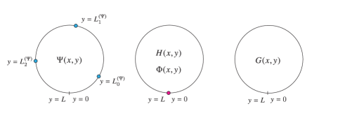
Figure 1: A schematic figure of the configuration of the point interactions. The fermions feel three point interactions, the gauge singlet scalar and the Higgs doublet feel one, the gauge fields do not feel the point interactions in the model.

Because of the point interactions, every field feels BC’s at its own positions. In our model, we adopt the following BC’s for the purpose.

$$L_{R} =0\hskip 30.00005pt{\rm at}\ \ \ y=L_{0}^{(L)},L_{1}^{(L)},L_{2}^{(L)},L_{3}^{(L)}\ ,$$ (9)

$${\cal N}_{L} =0\hskip 30.00005pt{\rm at}\ \ \ y=L_{0}^{({\cal N})},L_{1}^{({\cal N})},L_{2}^{({\cal N})},L_{3}^{({\cal N})}\ ,$$ (10)

$$E_{L} =0\hskip 30.00005pt{\rm at}\ \ \ y=L_{0}^{(E)},L_{1}^{(E)},L_{2}^{(E)},L_{3}^{(E)}\ .$$ (11)

$$\left\{\begin{array}[]{l}\Phi(x,0)+L_{+}\partial_{y}\Phi(x,0)=0,\\ \Phi(x,L)-L_{-}\partial_{y}\Phi(x,L)=0,\end{array}\right.\hskip 30.00005pt(-\infty\leq L_{\pm}\leq+\infty),$$ (14)

$$\left\{\begin{array}[]{l}H(x,L)=e^{i\theta}H(x,0){,}\\ \partial_{y}H(x,L)=e^{i\theta}\partial_{y}H(x,0),\end{array}\right.\hskip 30.00005pt(-\pi<\theta\leq\pi),$$ (17)

with the identification of $S^{1}$,

$$L \sim 0,$$ (18)

$$L_{3}^{({\cal N})} \sim L_{0}^{({\cal N})},$$ (19)

$$L_{3}^{(L)} \sim L_{0}^{(L)},$$ (20)

$$L_{3}^{(E)} \sim L_{0}^{(E)},$$ (21)

where the indices $R$ and $L$ of the fermions denote the 4d chirality defined as $\Psi_{R}\equiv\left(\frac{1+\gamma_{5}}{2}\right)\Psi,\ \Psi_{L}\equiv\left(\frac{1-\gamma_{5}}{2}\right)\Psi$ and $L_{\pm}$ are parameters which describe the Robin BC. A suitable choice of the parameters $L_{\pm}$ and other parameters in Eq. (4) makes the form of the VEV of the gauge-singlet hierarchical along the $y$-direction Fujimoto:2011kf ; Fujimoto:2012wv . Such a situation is preferable for generating the large hierarchy in the lepton mass matrices. $\theta$ is a phase parameter which specifies the twisted BC, whose complex degree of freedom is just the origin of CP violation in our model. We should emphasize that all the BC’s are consistent with the 5d gauge invariance. In particular, the BC’s (9)–(11) do not break the 5d gauge symmetry since the BC’s for the fermion are given by the Dirichlet BC, which is manifestly invariant under the 5d gauge transformation.

2.2 Generations

Since we put the BC’s (9)–(11) on the fermions with introducing the point interactions, three generations appears. The Kaluza-Klein (KK) expansion in this setup is done as

$$\Psi(x,y)=\sum_{n}\left(\psi^{(n)}_{R}(x)f^{(n)}_{\psi_{R}}(y)+\psi^{(n)}_{L}(x)g_{\psi_{L}}^{(n)}\right),$$ (22)

where $\{f_{\psi_{R}}^{(n)}\}$ $\Bigl{(}\{g_{\psi_{L}}^{(n)}\}\Bigr{)}$ is the eigenfunction of the hermitian operator $\mathcal{D}^{\dagger}\mathcal{D}$ $\left(\mathcal{D}\mathcal{D}^{\dagger}\right)$ and forms a complete set,

$$\left\{\begin{array}[]{l}\mathcal{D}^{\dagger}\mathcal{D}f_{\psi_{R}}^{(n)}=m^{2}_{\psi^{(n)}}f_{\psi_{R}}^{(n)},\\[5.69046pt] \mathcal{D}\mathcal{D}^{\dagger}g_{\psi_{L}}^{(n)}=m^{2}_{\psi^{(n)}}g_{\psi_{L}}^{(n)}{,}\end{array}\right.\hskip 30.00005pt(\mathcal{D}\equiv\partial_{y}+M_{\Psi},\ \mathcal{D}^{\dagger}\equiv-\partial_{y}+M_{\Psi}).$$ (25)

Zero mode solutions of the above should satisfy the following equations, which come from quantum mechanical supersymmetry.

$$\left\{\begin{array}[]{l}\mathcal{D}f_{\psi_{R}}^{(0)}=0,\\[5.69046pt] \mathcal{D}^{\dagger}g_{\psi_{L}}^{(0)}=0.\end{array}\right.$$ (28)

Non-trivial solution of the above is

$$\left\{\begin{array}[]{l}f_{\psi_{R}}^{(0)}\propto e^{-M_{\Psi}y},\\[5.69046pt] g_{\psi_{L}}^{(0)}\propto e^{+M_{\Psi}y}.\end{array}\right.$$ (31)

Furthermore, we imposed the BC’s in Eqs. (9)-(11) so that the three solutions appears to each segment. The situation is depicted in Fig 2.

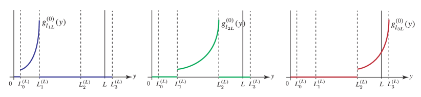
(a) The profiles of triply-degenerated zero modes $g_{l_{iL}}^{(0)}$ with $M_{L}>0$. (The profiles of $f_{\nu_{iR}}^{(0)}$, $f_{e_{iR}}^{(0)}$ with $M_{\cal N}$, $M_{E}<0$.)

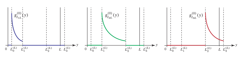
(b) The profiles of triply-degenerated zero modes $g_{l_{iL}}^{(0)}$ with $M_{L}<0$. (The profiles of $f_{\nu_{iR}}^{(0)}$, $f_{e_{iR}}^{(0)}$ with $M_{\cal N}$, $M_{E}>0$.)

Figure 2: A schematic figure of the zero modes.

Thus, we realize three generations in chiral zero modes in our model.

$$L(x,y) =\sum_{i=1}^{3}l^{(0)}_{iL}(x)g_{l_{iL}}^{(0)}(y)+({\rm KK\ modes}),$$ (32)

$${\cal N}(x,y) =\sum_{i=1}^{3}\nu^{(0)}_{iR}(x)f_{\nu_{iR}}^{(0)}(y)+({\rm KK\ modes}),$$ (33)

$$E(x,y) =\sum_{i=1}^{3}e^{(0)}_{iR}(x)f_{e_{iR}}^{(0)}(y)+({\rm KK\ modes}).$$ (34)

Note that the mode functions are localized toward the boundary points because of the bulk mass $M_{\Psi}$ ($\Psi=L,{\cal N},E$), the sign of whom determines the direction of the localization. We should note that the bulk mass controls all the related zero modes, so that we cannot change the form of the degenerated zero modes independently.

2.3 Charged lepton mass hierarchy and tiny neutrino masses

Under the action (1)–(5) with the BC’s (9)–(17), the lepton mass hierarchy and the tiny neutrino masses appear. The corresponding mass terms are generated through the following part.

$$S_{{\rm Yukawa}}^{({\rm lepton})}=\int d^{4}x\int^{L}_{0}dy\left[\Phi\Bigl{(}-{\cal Y}^{({\cal N})}\overline{L}(i\sigma_{2}H^{\ast}){\cal N}-{\cal Y}^{(E)}\overline{L}HE\Bigr{)}+({\rm h.c.})\right]$$

$$\quad{\supset-\int d^{4}x\sum_{i,j=1}^{3}\left[m_{ij}^{(\nu)}\overline{\nu_{iL}^{(0)}}\nu_{jR}^{(0)}+m_{ji}^{(\nu)}{}^{\ast}\overline{\nu_{jR}^{(0)}}\nu_{iL}^{(0)}\right]-\int d^{4}x\sum_{i,j=1}^{3}\left[m_{ij}^{(e)}\overline{e_{iL}^{(0)}}e_{jR}^{(0)}+m_{ji}^{(e)}{}^{\ast}\overline{e_{jR}^{(0)}}e_{iL}^{(0)}\right]},$$ (35)

where

$$m_{ij}^{(\nu)} ={\cal Y}^{({\cal N})}\int^{L}_{0}dy\,\langle h(y)\rangle^{\ast}\,\langle\Phi(y)\rangle\,g_{l_{iL}}^{(0)}(y)\,f_{\nu_{jR}}^{(0)}(y),$$ (36)

$$m_{ij}^{(e)} ={\cal Y}^{(E)}\int^{L}_{0}dy\,\langle h(y)\rangle\,\langle\Phi(y)\rangle\,g_{l_{iL}}^{(0)}(y)\,f_{e_{jR}}^{(0)}(y).$$ (37)

Under the Robin BC (14), it is known that the VEV of the gauge-singlet possesses the y-dependence and we can make it the exponential form by choosing suitable values of $L_{\pm}$, $M_{\Phi}$ and $\lambda_{\Phi}$ Fujimoto:2012wv ; Fujimoto:2011kf :

$$\langle\Phi(y)\rangle=\phi(y)\sim e^{M_{\Phi}y},$$ (38)

Obviously, the form of the VEV in Eq. (38) makes a big differences in the overlap integrals (37) and the exponential mass hierarchy appears for the charged leptons.

$$m_{11}^{(e)}\ll m_{22}^{(e)}\ll m_{33}^{(e)}.$$ (39)

On the other hand, this hierarchical structure does not appear in the neutrinos. In this model, we can obtain tiny neutrino masses of the order $m_{\nu}\sim{\cal O}(0.1)$eV with putting the value of the bulk masses as $M_{L}L$, $M_{{\cal N}}L$= ${\cal O}(100)$. In this situation, the immoderate localizations of the neutrino zero modes make the effect of the y-dependence of the gauge-singlet VEV $\langle\Phi(y)\rangle$ weak. Eventually the non-hierarchical mass structure appears in the neutrinos.

$$m_{11}^{(\nu)}\lesssim m_{22}^{(\nu)}\lesssim m_{33}^{(\nu)}.$$ (40)

2.4 Flavor Mixing

The source of the flavor mixing in this model is the off-diagonal components of the mass matrices (36)–(37). Since we introduce one extra-dimension, the way of the overlaps is restricted and we cannot fill up all components of the mass matrices. We found that only six components of the mass matrices are filled up. Under the following suitable choice of the configuration,

$$0<L_{0}^{({\cal N})}<L_{0}^{(L)}<L_{1}^{({\cal N})}<L_{1}^{(L)}<L_{2}^{({\cal N})}<L_{2}^{(L)}<L_{3}^{(N)}<L_{3}^{(L)},$$ (41)

$$0<L_{0}^{(L)}<L_{0}^{(E)}<L_{1}^{(E)}<L_{1}^{(L)}<L_{2}^{(E)}<L_{2}^{(L)}<L_{3}^{(L)}<L_{3}^{(E)},$$ (42)

the form of the mass matrices become like the following.

$$M^{(\nu)}=\left(\begin{array}[]{ccc}m_{11}^{(\nu)}&m_{12}^{(\nu)}&0\\[5.69046pt] 0&m_{22}^{(\nu)}&m_{23}^{(\nu)}\\[5.69046pt] m_{31}^{(\nu)}&0&m_{33}^{(\nu)}\end{array}\right),\hskip 30.00005ptM^{(e)}=\left(\begin{array}[]{ccc}m_{11}^{(e)}&m_{12}^{(e)}&m_{13}^{(e)}\\[5.69046pt] 0&m_{22}^{(e)}&m_{23}^{(e)}\\[5.69046pt] 0&0&m_{33}^{(e)}\end{array}\right).$$ (49)

A schematic figure of the configuration is depicted in Fig. 3.

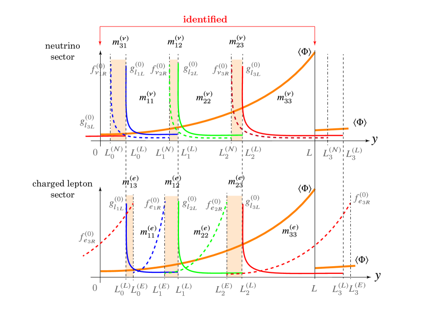
Figure 3: A schematic figure of the correspondence between the components of the mass matrices and the overlap integrals. The orange colored regions indicate the off-diagonal components of the mass matrices. $m_{ij}^{(\nu)}$ corresponds to the overlap of $g_{l_{iL}}^{(0)}$, $f_{\nu_{jR}}^{(0)}$ and $m_{ij}^{(e)}$ corresponds to that of $g_{l_{iL}}^{(0)}$ and $f_{e_{jR}}^{(0)}$.

The above restricted form of the mass matrices is convenient to reproduce the experimental values of the mixing angles and the lepton masses. We found that there is at least one parameter set in this setup, in which we can reproduce the experimental values with good precision under the configuration as we will see in the below.

2.5 CP phase

Since our model consists of one generation fermion in 5d, the Yukawa couplings cannot be a source of the CP phase. Then, the physical CP phase appears from the VEV of the Higgs, which possesses the following y-dependent phase due to the twisted BC (17) Fujimoto:2013ki .

$$\langle H(y)\rangle =\left(\begin{array}[]{c}0\\ \langle h(y)\rangle\end{array}\right)=\left(\begin{array}[]{c}0\\ v/\sqrt{2}\end{array}\right)e^{i\frac{\theta}{L}y},$$ (54)

Through the overlap integrals (36)–(37), the VEV of the Higgs provides a non-trivial phase to the mass matrix components. This phase can be a source of the physical CP phase and CP violation occurs in the PMNS matrix. We should emphasize that this Higgs VEV is the only source of the CP phase in our model, which implies that the magnitude of CP violation in the leptons can be a prediction after we adjust the CP phase of the quark sector.

2.6 Numerical results

As a typical example, we choose the parameters as

$$\tilde{L}_{0}^{(L)}=0.2565,\hskip 25.00003pt\tilde{L}_{1}^{(L)}=0.5776,\hskip 20.00003pt\tilde{L}_{2}^{(L)}=0.9432,$$

$$\tilde{L}_{0}^{({\cal N})}=0.08240,\hskip 16.00008pt\tilde{L}_{1}^{({\cal N})}=0.3909,\hskip 18.00005pt\tilde{L}_{2}^{({\cal N})}=0.7317,$$

$$\tilde{L}_{0}^{(E)}=0.277,\hskip 28.99997pt\tilde{L}_{1}^{(E)}=0.49,\hskip 30.00005pt\tilde{L}_{2}^{(E)}=0.79,$$

$$\tilde{M}_{L}=-136.9,\hskip 18.99995pt\tilde{M}_{{\cal N}}=112.1,\hskip 18.99995pt\tilde{M}_{E}=-2.00,$$

$$\tilde{M}_{\Phi}=8.67,\hskip 22.0pt\tilde{\lambda}_{\Phi}={0.001},\hskip 22.0pt\frac{1}{\tilde{L}_{+}}=-6.07,\hskip 10.00002pt\frac{1}{\tilde{L}_{-}}=8.69,\hskip 28.00006pt\theta=3,$$

$${\tilde{{\cal Y}}^{(\mathcal{N})}}=-0.0000309-9.15\times 10^{-6}\,i,\hskip 20.00003pt{\tilde{{\cal Y}}^{(E)}}=-0.00309-0.000915\,i$$ (55)

where the variables with   $\tilde{}\$ are dimensionless parameters, which are scaled by using the circumference $L$ of the extra dimension. By calculating the mass eigenvalues, the PMNS matrix and the Jarlskog parameter in the leptonic sector $J_{{\rm lepton}}$ through the overlap integrals (36)–(37), the following values are obtained.

$${m_{\nu_{1}}}=0.0092\ {\rm eV},\hskip 38.00008pt{m_{\nu_{2}}}=0.013\ {\rm eV},\hskip 33.99998pt{m_{\nu_{3}}}={0.018}\ {\rm eV},$$

$$m_{{\rm electron}}={0.519}\ {\rm MeV},\hskip 18.00005ptm_{{\rm muon}}={106}\ {\rm MeV},\hskip 23.99997ptm_{{\rm tau}}={1.778}\ {\rm GeV},$$

$$\sin^{2}\theta_{12}={0.333},\hskip 20.00003pt\sin^{2}\theta_{23}={0.435},\hskip 20.00003pt\sin^{2}\theta_{13}={0.0239},$$

$$J_{{\rm lepton}}={0.0214}\ \ (\sin\delta={0.607}).$$ (56)

The ratio between the above results and the experimental results are shown in the follows:

$$\sqrt{\frac{\delta m^{2}}{\delta m^{2}{}^{({\rm exp.)}}}}={1.03},\hskip 28.00006pt\sqrt{\frac{\Delta m^{2}}{\Delta m^{2}{}^{({\rm exp.)}}}}={0.285},$$

$$\frac{m_{{\rm electron}}}{m_{{\rm electron}}^{({\rm exp.})}}=1.02,\hskip 28.00006pt\frac{m_{{\rm muon}}}{m_{{\rm muon}}^{({\rm exp.})}}=0.995,\hskip 26.00009pt\frac{m_{{\rm tau}}}{m_{{\rm tau}}^{({\rm exp.})}}=1.00,$$

$$\frac{\sin^{2}\theta_{{\rm 12}}}{\sin^{2}\theta_{{\rm 12}{}^{({\rm exp.})}}}={1.08},\hskip 28.00006pt\frac{\sin^{2}\theta_{{\rm 23}}}{\sin^{2}\theta_{{\rm 23}{}^{({\rm exp.})}}}={1.02},\hskip 26.00009pt\frac{\sin^{2}\theta_{{\rm 13}}}{\sin^{2}\theta_{{\rm 13}{}^{({\rm exp.})}}}={1.02},$$ (57)

where we defined $\delta m^{2}$ and $\Delta m^{2}$ as

$$\delta m^{2}\equiv m_{\nu_{2}}^{2}-m_{\nu_{1}}^{2},$$ (58)

$$\Delta m^{2}\equiv m_{\nu_{3}}^{2}-\left(\frac{m_{\nu_{1}}^{2}{+}m_{\nu_{2}}^{2}}{2}\right),$$ (59)

according to Ref. Capozzi:2013csa . The mixing angles of the PMNS matrix are within the 3$\sigma$ range Capozzi:2013csa . The value of $\sqrt{\frac{\Delta m^{2}}{\Delta m^{2({\rm exp.})}}}$ in our example is slightly smaller than experimental range, i.e. about factor-four. An exhaustive parameter scanning would help us to find a rather reasonable point.

3 Summary and Discussions

We investigated the 5d gauge theory on $S^{1}$ with point interactions. The BC’s and the suitable choice of the parameters provide three generations, the charged lepton mass hierarchy, the lepton flavor mixing and tiny degenerated neutrino masses. The magnitude of the CP violation in the lepton sector can be a prediction and other physical quantities are reproduced with good precision in our model.

References

• (1) M. Kobayashi, T. Maskawa, Prog.Theor.Phys. 49, 652 (1973)
• (2) Y. Fujimoto, T. Nagasawa, K. Nishiwaki, M. Sakamoto, PTEP 2013, 023B07 (2013), 1209.5150
• (3) Y. Fujimoto, K. Nishiwaki, M. Sakamoto, R. Takahashi, JHEP 1410, 191 (2014), 1405.5872
• (4) M. Reed, B. Simon, Methods of Modern Mathematical Physics. 2. Fourier Analysis, Selfadjointness (1975)
• (5) P. Seva, J. of Phys 36, 667 (1986)
• (6) T. Cheon, T. Fulop, I. Tsutsui, Annals Phys. 294, 1 (2001), quant-ph/0008123
• (7) Y. Fujimoto, K. Nishiwaki, M. Sakamoto, Phys.Rev. D88, 115007 (2013), 1301.7253
• (8) Y. Fujimoto, T. Nagasawa, S. Ohya, M. Sakamoto, Prog.Theor.Phys. 126, 841 (2011), 1108.1976
• (9) F. Capozzi, G. Fogli, E. Lisi, A. Marrone, D. Montanino et al., Phys.Rev. D89, 093018 (2014), 1312.2878