Consistency of the light-front quark model with chiral symmetry in the pseudoscalar meson analysis

Abstract

We discuss the link between the chiral symmetry of QCD and the numerical results of the light-front quark model (LFQM), analyzing both the two-point and three-point functions of a pseudoscalar meson from the perspective of the vacuum fluctuation consistent with the chiral symmetry of QCD. The two-point and three-point functions are exemplified in this work by the twist-2 and twist-3 distribution amplitudes of a pseudoscalar meson and the pion elastic form factor, respectively. The present analysis of the pseudoscalar meson commensurates with the previous analysis of the vector meson two-point function and fortifies our observation that the light-front quark model with effective degrees of freedom represented by the constituent quark and antiquark may provide the view of effective zero-mode cloud around the quark and antiquark inside the meson. Consequently, the constituents dressed by the zero-mode cloud may be expected to satisfy the chiral symmetry of QCD. Our results appear consistent with this expectation and effectively indicate that the constituent quark and antiquark in the LFQM may be considered as the dressed constituents including the zero-mode quantum fluctuations from the vacuum.

I Introduction

Hadronic distribution amplitudes (DAs) provide essential information on the QCD interaction of quarks, antiquarks and gluons inside the hadrons and play an essential role in applying QCD to hard exclusive processes. They are the longitudinal projection of the hadronic wave functions obtained by integrating the transverse momenta of the fundamental constituents BL80 ; ER80 ; CZ84 . These nonperturbative quantities are defined as vacuum-to-hadron matrix elements of particular nonlocal quark or quark-gluon operators and thus encode important information on bound states in strong interaction physics. It has motivated many studies using various nonperturbative models BF ; Ball99 ; BBL ; CJ_DA ; PR ; NK06 ; HWZ04 ; HZW05 and led to develop distinct phenomenological models over the past two decades. Among them, the light-front quark model (LFQM) appears to be one of the most efficient and effective tools in hadron physics as it takes advantage of the distinguished features of the light-front dynamics (LFD) BPP . In particular, the LFD carries the maximum number (seven) of the kinetic (or interaction independent) generators and thus the less effort in dynamics is necessary in order to get the QCD solutions that reflect the full Poincar$\acute{e}$ symmetries. Moreover, the rational energy-momentum dispersion relation of LFD, namely $p^{-}=({\bf p}^{2}_{\perp}+m^{2})/p^{+}$, yields the sign correlation between the LF energy $p^{-}(=p^{0}-p^{3})$ and the LF longitudinal momentum $p^{+}(=p^{0}+p^{3})$ and leads to the suppression of quantum fluctuations of the vacuum, sweeping the complicated vacuum fluctuations into the zero-modes in the limit of $p^{+}\rightarrow 0$ Zero1 ; Zero2 ; Zero3 . This simplification is a remarkable advantage in LFD and facilitates the partonic interpretation of the amplitudes. Based on the advantages of the LFD, the LFQM has been developed CJ_99 and subsequently applied for various meson phenomenologies such as the mass spectra of both heavy and light mesons CJ_Bc , the decay constants, DAs, form factors and generalized parton distributions Jaus90 ; Jaus99 ; Jaus03 ; Cheng04 ; CJ_99 ; CJ_DA ; Choi07 ; BPP ; MF12 ; CJ_Bc ; CJ_PV .

Despite these successes in reproducing the general features of the data, however, it has proved very difficult to obtain direct connection between the LFQM and QCD. To discuss the link between the chiral symmetry of QCD and the numerical results of the LFQM, we recently presented a self-consistent covariant description of vector meson decay constants and chirality-even quark-antiquark DAs up to twist 3 in LFQM CJ_V14 . Although the meson decay amplitude described by a two-point function could be regarded as one of the simplest possible physical observables, it is interesting that this apparently simple amplitude bears abundant fundamental information on QCD vacuum dynamics and chiral symmetry. In particular, we discussed the zero-mode issue in the LFQM prediction of vector meson decay constants from the perspective of the vacuum fluctuation consistent with the chiral symmetry of QCD and extended the exactly solvable manifestly covariant Bethe-Salpeter (BS) model calculation to the more phenomenologically accessible realistic LFQM.

To discuss the nature of the LF zero-mode in meson decay amplitude, we may denote the total LF longitudinal momentum of the meson, $P^{+}=k_{Q}^{+}+k_{\bar{Q}}^{+}$, where $k_{Q}^{+}$ and $k_{\bar{Q}}^{+}$ are the individual quark and antiquark LF longitudinal momenta, respectively. Similarly, the total LF energy $P^{-}$ is shared by the individual quark and antiquark LF energies $k_{Q}^{-}$ and $k_{\bar{Q}}^{-}$, i.e. $P^{-}=k_{Q}^{-}+k_{\bar{Q}}^{-}$. For the LF energy integration of the two-point function over $k_{Q}^{-}$ or $k_{\bar{Q}}^{-}$ to compute the meson decay amplitude, one may use the Cauchy’s theorem for a contour integration and pick up the LF energy pole, e.g. either $[k_{Q}^{-}]_{\rm on}$ (i.e. on-shell value of $k_{Q}^{-}$) from the quark propagator or $[k_{\bar{Q}}^{-}]_{\rm on}$ from the antiquark propagator. However, it is crucial to note that the poles move to infinity (or fly away in the complex plane) as the LF longitudinal momentum, either $k_{Q}^{+}$ or $k_{\bar{Q}}^{+}$, goes to zero BDJM . Unless the contribution from the pole flown into infinity vanishes, it must be kept in computing the physical observable that must reflect the full Poincar$\acute{e}$ symmetries. Since such contribution, if it exists, appears either from $k_{Q}^{+}=0$ and $k_{\bar{Q}}^{+}=P^{+}$ or from $k_{\bar{Q}}^{+}=0$ and $k_{Q}^{+}=P^{+}$, we call it as the zero-mode contribution. In the case of two-point function for the computation of the meson decay constant, the zero-mode contribution is thus locked into a single point of the LF longitudinal momentum, i.e. either $k_{Q}^{+}=0$ where $k_{\bar{Q}}^{+}=P^{+}$ or $k_{\bar{Q}}^{+}=0$ where $k_{Q}^{+}=P^{+}$. As one of the constituents of the meson carries the entire momentum $P^{+}$ of the meson in this case, the other constituent carries the zero LF longitudinal momentum that can be regarded as the zero-mode quantum fluctuation linked to the vacuum. This link is due to a pair creation of particles with zero LF longitudinal momenta from the vacuum and it is important to capture the vacuum effect for the consistency with the chiral symmetry properties of the strong interactions JMT2013 . With this link, the zero-mode contribution in the meson decay process can be considered effectively as the effect of vacuum fluctuation consistent with the chiral symmetry of the strong interactions. In this respect, the LFQM with effective degrees of freedom represented by the constituent quark and antiquark may be linked to the QCD since the zero-mode link to the QCD vacuum may provide the view of an effective zero-mode cloud around the quark and antiquark inside the meson. Although the constituents are dressed by the zero-mode cloud, they are still expected to satisfy the chiral symmetry consistent with the QCD. Our numerical results CJ_V14 were indeed consistent with this expectation and effectively indicated that the constituent quark and antiquark in the standard LFQM CJ_99 ; CJ_DA ; Choi07 ; Jaus90 ; Cheng97 ; Hwang10 ; Kon could be considered as the dressed constituents including the zero-mode quantum fluctuations from the QCD vacuum.

Since the constituent quark and antiquark used in the LFQM have already absorbed the zero-mode cloud, the zero-mode contribution in the LFQM may not be as explicit as in the manifestly covariant model calculation although it effectively provides the consistency with the chiral symmetry. The standard light-front (SLF) approach of the LFQM, with which the observables are directly computed in 3-dimensional LF momentum space, is not amenable to determine the zero-mode contribution by itself and thus it has been a common practice to utilize an exactly solvable manifestly covariant BS model to check the existence (or absence) of the zero-mode as one can pin down the zero mode exactly in the manifestly covariant BS model. Within the covariant BS model, we indeed found the nonvanishing zero modes in the vector meson decay amplitude and identified the corresponding zero-mode operators that can be applied to the LFQM. We also found the self-consistent correspondence relations (see e.g. Eq. (49) in CJ_V14 ) between the covariant BS model and the LFQM that allow the substitution of the radial and spin-orbit wave functions of the exactly solvable model by the more phenomenologically accessible model wave functions that can be provided by the LFQM analysis of meson masses CJ_99 . What is remarkable in our finding CJ_V14 is that the nonvanishing zero-mode contributions as well as the instantaneous ones to the vector meson decay amplitude appeared in the covariant BS model now vanish explicitly when the phenomenological wave function such as the Gaussian wave function in LFQM is used through the aforementioned correspondence relation. In another words, the decay constants and the quark DAs of vector mesons can be obtained only from the on-mass-shell valence contribution within the framework of the standard LFQM CJ_99 ; Kon ; Jaus90 ; Jaus91 ; Cheng97 ; CCP ; Card95 ; Hwang10 ; CJK02 ; Choi07 using the Gaussian radial wave function and they still satisfy the chiral symmetry consistent with the QCD.

One of the key ingredients for this finding is the isospin symmetry, namely, the symmetric DAs for the equal quark and antiquark bound state mesons (e.g. $\rho$ meson). Under the exchange of the LF longitudinal momentum fraction of the quark and antiquark, $x\leftrightarrow(1-x)$, the DA of the meson with the two equal-mass constituents must be symmetric, $\phi(x)=\phi(1-x)$. We exploited this fundamental constraint anticipated from the isospin symmetry to identify the correct DAs in LFQM. The twist-2 and twist-3 DAs of the $\rho$ meson obtained only from the on-mass-shell valence constituents in LFQM CJ_V14 not only satisfy this constraint anticipated from the isospin symmetry but also reproduce the correct asymptotic DAs in the chiral symmetry limit. Knowing that the higher-twist DAs may come from the contributions of the higher Fock-states such as pair terms as well as the transverse motion of constituents in the leading twist components BF ; Ball99 ; BBL , we should further attest that our LFQM formulation for the twist-3 DA is indeed simple without involving zero modes and thus the connected contributions to the current arising from the vacuum disappear in our LFQM calculation, yet preserves all the necessary constraints anticipated from the isospin symmetry and the chiral symmetry.

The purpose of this work is to extend our previous work to analyze the decay amplitude related with twist-3 DAs of a pseudoscalar meson within the LFQM and show that the analysis of pseudoscalar mesons fortify our previous conclusion drawn from the vector meson case CJ_V14 . That is, the treacherous points such as the zero-mode and the instantaneous contributions present in the covariant BS model disappear in the standard LFQM with the Gaussian radial wave function but nevertheless satisfy the chiral symmetry. The twist-3 DAs of a pseudoscalar meson appear to play an important role in constraining our LFQM to be consistent with the conclusion drawn from our previous analysis of the vector meson decay constant. The twist-2 DA of a pseudoscalar meson has been analyzed in our previous work of LFQM CJ_DA . Essentially, there are two independent twist-3 two-particle DAs of a pseudoscalar meson, namely, $\phi^{\cal P}_{3;M}$ and $\phi^{\sigma}_{3;M}$ BF ; Ball99 ; BBL ; PR ; NK06 ; HWZ04 ; HZW05 corresponding to pseudoscalar and tensor channels of a meson ($M$), respectively. In this work, we shall study $\phi^{\cal P}_{3;M}$ together with the twist-2 DA $\phi^{\cal A}_{2;M}$ corresponding to the axial-vector channel for the sake of completeness.

The $\phi^{\cal A}_{2;M}$ and $\phi^{\cal P}_{3;M}$ are defined in terms of the following matrix elements of gauge invariant nonlocal operators at light-like separation BF ; Ball99 ; BBL :

$$\langle 0|{\bar{q}}(z)[z,-z]\gamma^{\mu}\gamma_{5}q(-z)|M(P)\rangle=if_{M}P^{\mu}\int^{1}_{0}dxe^{i\zeta P\cdot z}\phi^{\cal A}_{2;M}(x),$$ (1)

and

$$\langle 0|{\bar{q}}(z)[z,-z]i\gamma_{5}q(-z)|M(P)\rangle=f_{M}\mu_{M}\int^{1}_{0}dxe^{i\zeta P\cdot z}\phi^{\cal P}_{3;M}(x),$$ (2)

where $z^{2}=0$ and the path-ordered gauge link (Wilson line) $[z,-z]$ for the gluon fields between the points $-z$ and $z$ is equal to unity in the light-cone gauge $A(z)\cdot z=0$ which we take throughout our calculation. $P$ is the four-momentum of the meson ($P^{2}=m^{2}_{M}$) and the integration variable $x$ corresponds to the longitudinal momentum fraction carried by the quark and $\zeta=2x-1$ for the short-hand notation. The normalization parameter $\mu_{M}=m^{2}_{M}/(m_{q}+m_{\bar{q}})$ in Eq. (2) results from quark condensate. For the pion, $\mu_{\pi}=-2\langle{\bar{q}}q\rangle/f^{2}_{\pi}$ from the Gell-Mann-Oakes-Renner relation GOR . The normalization of the two DAs $\Phi=\{\phi^{\cal A}_{2;M},\phi^{\cal P}_{3;M}\}$ is given by

$$\int^{1}_{0}dx\;\Phi(x)=1.$$ (3)

In order to check the existence (or absence) of the zero mode, we again utilize the same manifestly covariant model used in the analysis of the vector meson decay constant CJ_V14 and then substitute the vertex function with the more phenomenologically accessible Gaussian radial wave function provided by our LFQM. We shall show that the analysis of the decay constants and twist-2 and twist-3 two-particle DAs of pseudoscalar mesons confirms our previous conclusion drawn for the vector meson analysis CJ_V14 . Namely, the treacherous points such as the zero-mode and the instantaneous contributions appeared in the covariant BS model do not show up explicitly in the standard LFQM with the Gaussian radial wave function but nevertheless satisfy the chiral symmetry.

In addition, we show that our findings of the zero-mode complication in two-point function is directly applicable to the three-point function with the analysis of the pion elastic form factor. The analyses of the pion form factor using the plus component ($J^{+}_{\rm em}$) of the LF currents have been done in many earlier works BCJ01 ; CJK ; CJ06 ; CJ08 and proved that the pion form factor is immune to the zero-mode contribution when the plus component of the currents is used. Particularly, in our LFQM analysis of the pion form factor CJ06 ; CJ08 , we have shown that the usual power-law behavior of the pion form factor obtained in the perturbative QCD analysis can also be attained by taking negligible quark masses in our nonperturbative LFQM analysis, confirming the anti-de Sitter space geometry/conformal field theory (AdS/CFT) correspondence BT04 . In this work, we analyze the pion form factor using the perpendicular components ($J^{\perp}_{\rm em}$) of the currents. Within the covariant BS model, we find that the form factor obtained in the $q^{+}=0$ frame with $J^{\perp}_{\rm em}$ receives only the valence contribution including both the on-mass-shell quark propagating part and the off-mass-shell instantaneous part without involving a zero mode. Applying this to the LFQM, we find that the nonvanishing instantaneous contribution appeared in the BS model does not appear and just the on-mass-shell propagating part contributes in the LFQM. This example of the three-point function provides an evidence that the conclusion drawn in the LFQM analysis of the two-point function is also applicable to the three-point function.

The paper is organized as follows. In Sec. II.1, we discuss the decay amplitude of a pseudoscalar meson described by the two-point function and the pion form factor described by three-point function in an exactly solvable model based on the covariant BS model of (3+1)-dimensional fermion field theory. We mainly perform our LF calculation for the decay amplitude corresponding to the twist-3 DA $\phi^{\cal P}_{3;M}$ and the pion form factor using $J^{\perp}_{\rm em}$ and check the LF covariance of them within the covariant BS model. Especially, we discuss how to identify the zero-mode contribution and find the corresponding zero-mode operator. In Sec. III, we present the standard LFQM with the gaussian wave function and discuss the correspondence linking the manifestly covariant model to the standard LFQM. The self-consistent covariant descriptions of the meson decay constants as well as the twist-2 and twist-3 two-particle DAs of pseudoscalar mesons in the standard LFQM are given in this section. In Sec. IV, we present our numerical results for the explicit demonstration of our findings. Summary and discussion follow in Sec. V.

II Manifestly Covariant Model

II.1 Two-point function: decay amplitude

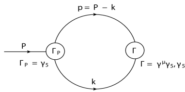
Figure 1: Feynman diagram for the one-quark-loop evaluation of the meson decay amplitude in the momentum space.

Defining the local matrix elements ${\cal M}_{\alpha}\equiv\langle 0|{\bar{q}}\Gamma_{\alpha}q|M(P)\rangle(\alpha={\cal A,P})$ for axial-vector ($\Gamma_{\cal A}=\gamma^{\mu}\gamma_{5}$) and pseudoscalar ($\Gamma_{\cal P}=i\gamma_{5}$) channels of Eqs. (1) and (2), we write the one-loop approximation (see Fig. 1) as a momentum integral

$${\cal M}_{\alpha}=N_{c}\int\frac{d^{4}k}{(2\pi)^{4}}\frac{H_{0}}{N_{p}N_{k}}S_{\alpha},$$ (4)

where $N_{c}$ denotes the number of colors. The denominators $N_{p}(=p^{2}-m^{2}_{q}+i\varepsilon)$ and $N_{k}(=k^{2}-m^{2}_{\bar{q}}+i\varepsilon)$ come from the quark propagators of mass $m_{q}$ and $m_{\bar{q}}$ carrying the internal four-momenta $p=P-k$ and $k$, respectively. In order to regularize the covariant loop, we use the usual multipole ansatz Jaus99 ; CJ_V14 ; MF97 ; SS for the $q{\bar{q}}$ bound-state vertex function $H_{0}=H_{0}(p^{2},k^{2})$ of a meson:

$$H_{0}(p^{2},k^{2})=\frac{g}{N_{\Lambda}^{n}},$$ (5)

where $N_{\Lambda}=p^{2}-\Lambda^{2}+i\varepsilon$, and $g$ and $\Lambda$ are constant parameters. Although the vertex function $H_{0}$ could be symmetrized in the four momenta of the constituent quarks for further study, we take a simplest possible regularization in this work as a tool to analyze the zero-mode complication in the exactly solvable model. In the same vein, although the power $n$ for the multipole ansatz could be $n\geq 2$ to regularize the loop integral, we take the lowest possible power $n=2$ since our qualitative results in terms of the zero-mode issue do not depend on the value of $n$.

The trace term $S_{\alpha}$ in Eq. (4) is given by

$$S_{\alpha}={\rm Tr}\left[\Gamma_{\alpha}\left(/\!\!\!p+m_{q}\right)\gamma_{5}\left(-/\!\!\!k+m_{\bar{q}}\right)\right].$$ (6)

We have already computed the matrix element ${\cal M_{A}}$ of the axial-vector channel in the Appendix B of Ref. CJ_V14 and have shown that ${\cal M_{A}}$ (i.e. the decay constant of a pseudoscalar meson) obtained from the plus component of the currents is immune to the zero mode. Therefore, we shall discuss the pseudoscalar channel and the associated twist-3 DA $\phi^{\cal P}_{3;M}$ in this work. After a little manipulation, we obtain the manifestly covariant result for ${\cal M_{P}}$ as follows

$${\cal M}_{\cal P}^{\rm cov} = \frac{N_{c}g}{4\pi^{2}}\int^{1}_{0}dx\int^{1-x}_{0}dy(1-x-y)\biggl{\{}\frac{y(1-y)m^{2}_{M}+m_{q}m_{\bar{q}}}{C^{2}_{\rm cov}}-\frac{2}{C_{\rm cov}}\biggr{\}},$$ (7)

where $C_{\rm cov}=y(1-y)m^{2}_{M}-xm^{2}_{q}-ym^{2}_{\bar{q}}-(1-x-y)\Lambda^{2}$.

For the LF calculation in parallel with the manifestly covariant one, we separate the trace term $S_{\cal P}$ in Eq. (6) into the on-mass-shell propagating part $[S_{\cal P}]_{\rm on}$ and the off-mass-shell instantaneous part $[S_{\cal P}]_{\rm inst}$ via $/\!\!\!q=/\!\!\!q_{\rm on}+\frac{1}{2}\gamma^{+}(q^{-}-q^{-}_{\rm on})$ as

$$S_{\cal P}=[S_{\cal P}]_{\rm on}+[S_{\cal P}]_{\rm inst},$$ (8)

where $[S_{\cal P}]_{\rm on}=4(p_{\rm on}\cdot k_{\rm on}+m_{q}m_{\bar{q}})$ and $[S_{\cal P}]_{\rm inst}=2(p^{+}\Delta_{k}^{-}+k^{+}\Delta_{p}^{-})$ with $\Delta_{q}^{-}=q^{-}-q_{\rm on}^{-}$. We note that the metric convention $a\cdot b=\frac{1}{2}(a^{+}b^{-}+a^{-}b^{+})-{\bf a}_{\perp}\cdot{\bf b}_{\perp}$ is used in our analysis. Furthermore, we take the reference frame where ${\bf P}_{\perp}=0$, i.e., $P=(P^{+},M^{2}/P^{+},0)$. In this case, the LF energies of the on-mass-shell quark and antiquark are given by $p^{-}_{\rm on}=({\bf k}^{2}_{\perp}+m^{2}_{q})/xP^{+}$ and $k^{-}_{\rm on}=({\bf k}^{2}_{\perp}+m^{2}_{\bar{q}})/(1-x)P^{+}$, respectively, where $x=p^{+}/P^{+}$ is the LF longitudinal momentum fraction of the quark.

For the integration over $k^{-}$ in Eq. (4), one may close the contour in the lower half of the complex $k^{-}$ plane and pick up the residue at $k^{-}=k^{-}_{\rm on}$ in the region $0<k^{+}<P^{+}$ (or $0<x<1$). We denote the valence contribution to ${\cal M_{P}}$ which is obtained by taking $k^{-}=k^{-}_{\rm on}$ in the region of $0<x<1$ as $[{\cal M_{P}}]^{\rm LF}_{\rm val}$ that is given by

$$[{\cal M_{P}}]^{\rm LF}_{\rm val}=\frac{N_{c}}{16\pi^{3}}\int^{1}_{0}\frac{dx}{(1-x)}\int d^{2}{\bf k}_{\perp}\chi(x,{\bf k}_{\perp})[S_{\cal P}]_{\rm val},$$ (9)

where

$$\chi(x,{\bf k}_{\perp})=\frac{g}{[x(m_{M}^{2}-M^{2}_{0})][x(m_{M}^{2}-M^{2}_{\Lambda})]^{n}},$$ (10)

with $n=2$ and

$$M^{2}_{0(\Lambda)} = \frac{{\bf k}^{2}_{\perp}+m^{2}_{q}(\Lambda^{2})}{x}+\frac{{\bf k}^{2}_{\perp}+m^{2}_{\bar{q}}}{1-x}.$$ (11)

Here, the trace term for the valence contribution, i.e. $[S_{\cal P}]_{\rm val}=[S_{\cal P}]_{\rm on}+2k^{+}\Delta_{p}^{-}$, is given by

$$[S_{\cal P}]_{\rm val}=2[M^{2}_{0}-(m_{q}-m_{\bar{q}})^{2}+(1-x)E_{\rm E.B.}],$$ (12)

where the binding energy term $E_{\rm E.B.}=m^{2}_{M}-M^{2}_{0}$ stems from the instantaneous contribution. We find numerically that $[{\cal M_{P}}]^{\rm LF}_{\rm val}$ in Eq. (9) is not identical to the manifestly covariant result ${\cal M_{P}}^{\rm cov}$ in Eq. (7). This indicates that the decay amplitude ${\cal M_{P}}$ receives the LF zero-mode contribution. The LF zero-mode contribution to ${\cal M_{P}}$ comes from the singular $p^{-}$ (or equivalently $1/x$) term in $S_{\cal P}$ in the limit of $x\to 0$ when $p^{-}=p^{-}_{\rm on}$, i.e.

$$\lim_{x\to 0}S_{\cal P}(p^{-}=p^{-}_{\rm on})=2p^{-}.$$ (13)

The necessary prescription to identify zero-mode operator corresponding to $p^{-}$ is analogous to that derived in the previous analyses of weak transition form factor calculations Jaus99 ; CJ_Bc ; CJ_PV , except that there is no momentum transfer $q$ dependence. As extensively discussed in the previous works Jaus99 ; CJ_Bc ; CJ_PV ; CJ_V14 , we now identify the zero-mode operator $[S_{\cal P}]_{\rm Z.M.}$ by replacing $p^{-}$ with $-Z_{2}$ in Eq. (13), i.e.

$$[S_{\cal P}]_{\rm Z.M.}=2(-Z_{2}),$$ (14)

where $Z_{2}=xE_{\rm E.B.}+m^{2}_{q}-m^{2}_{\bar{q}}+(1-2x)m_{M}^{2}$. This zero-mode operator $[S_{\cal P}]_{\rm Z.M.}$ can be effectively included in the valence region as follows

$$[{\cal M_{P}}]^{\rm LF}_{\rm full} = \frac{N_{c}}{16\pi^{3}}\int^{1}_{0}\frac{dx}{(1-x)}\int d^{2}{\bf k}_{\perp}\chi(x,{\bf k}_{\perp})[S_{\cal P}]_{\rm full},$$ (15)

where $[S_{\cal P}]_{\rm full}=[S_{\cal P}]_{\rm val}+[S_{\cal P}]_{\rm Z.M.}$ and it is given by

$$[S_{\cal P}]_{\rm full}=4[xM^{2}_{0}+m_{q}(m_{\bar{q}}-m_{q})].$$ (16)

It can be checked that Eq. (15) is identical to the manifestly covariant result of Eq. (7).

Although the amplitude ${\cal M_{A}}=if_{M}P^{\mu}$ for the axial vector channel is proven to be immune to the zero mode when the plus component ($\mu=+$) of the currents is used and its form is given in Ref. CJ_V14 , we display it here again for completeness in the form of a pseudoscalar meson decay constant:

$$f^{\rm LF}_{M}=\frac{N_{c}}{4\pi^{3}}\int^{1}_{0}\frac{dx}{(1-x)}\int d^{2}{\bf k}_{\perp}\chi(x,{\bf k}_{\perp}){\cal A},$$ (17)

where ${\cal A}=(1-x)m_{q}+xm_{\bar{q}}$.

II.2 Three-point function: Pion electromagnetic form factor

The electromagnetic form factor of a pion is defined by the matrix elements of the current $J^{\mu}_{\rm em}$:

$$\langle P^{\prime}|J^{\mu}_{\rm em}|P\rangle=e_{m}(P+P^{\prime})^{\mu}F_{\pi}(q^{2}),$$ (18)

where $e_{m}$ is the charge of the meson and $q^{2}=(P-P^{\prime})^{2}$ is the square of the four momentum transfer.

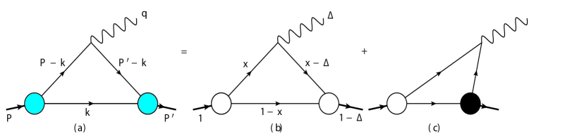
Figure 2: The covariant triangle diagram (a) corresponds to the sum of the LF valence diagram (b) and the nonvalence diagram (c). The large white and black blobs at the meson-quark vertices in (b) and (c) represent the ordinary LF wave function and the nonvalence wave function vertices, respectively.

The covariant diagram shown in Fig. 2(a) to describe the pion form factor is in general equivalent to the sum of the LF valence diagram [Fig. 2(b)] and the nonvalence diagram [Fig. 2(c)]. The matrix element ${\cal J}^{\mu}\equiv\langle P^{\prime}|J^{\mu}_{\rm em}|P\rangle$ obtained from the covariant diagram of Fig. 2(a) is given by

$${\cal J}^{\mu}=iN_{c}\int\frac{d^{4}k}{(2\pi)^{4}}\frac{H^{\prime}_{0}H^{\prime\prime}_{0}}{N_{p_{1}}N_{k}N_{p_{2}}}S^{\mu},$$ (19)

where

$$S^{\mu}={\rm Tr}[\gamma_{5}(\not\!p_{1}+m)\gamma^{\mu}(\not\!p_{2}+m)\gamma_{5}(-\not\!k+m)]$$ (20)

with $p_{1}=P-k$ and $p_{2}=P^{\prime}-k$. Here, we take $m_{q}=m_{\bar{q}}=m$ for the pion. The vertex functions are given by $H^{\prime}_{0}=H^{\prime}_{0}(p^{2}_{1},k^{2})=g/(N^{\prime}_{\Lambda})^{n}$ and $H^{\prime\prime}_{0}=H^{\prime\prime}_{0}(p^{2}_{2},k^{2})=g/(N^{\prime\prime}_{\Lambda})^{n}$ with $N^{\prime}_{\Lambda}(N^{\prime\prime}_{\Lambda})=p_{1}^{2}(p_{2}^{2})-\Lambda^{2}+i\epsilon$. In this case, we take the power $n$ for the multipole ansatz to be simply 1, since our qualitative results in conjunction with the zero-mode issue do not depend on the value of $n$. The rest of the denominator factor $N_{p}$ from the intermediate quark propagator with momentum $p=(p_{1},p_{2},k)$ is given by $N_{p}=p^{2}-m^{2}+i\epsilon$.

Using the usual Feynman parametrization, we obtain the manifestly covariant result as follows

$$F^{\rm cov}_{\pi}(q^{2}) = \frac{N_{c}g^{2}}{8\pi^{2}(\Lambda^{2}-m^{2})^{2}}\int^{1}_{0}dx\int^{1-x}_{0}dy\biggl{\{}[3(x+y)-4]\ln\biggl{(}\frac{C_{\Lambda m}C_{m\Lambda}}{C_{mm}C_{\Lambda\Lambda}}\biggr{)}$$ (21)

$$+[(1-x-y)^{2}(x+y)m_{\pi}^{2}+xy(2-x-y)q^{2}-(x+y)m^{2}+2m^{2}]C\biggr{\}},$$

where $C=(1/C_{\Lambda\Lambda}-1/C_{\Lambda m}-1/C_{m\Lambda}+1/C_{mm})$ and $C_{ab}=(1-x-y)(x+y)m_{\pi}^{2}+xyq^{2}-(xa^{2}+yb^{2})-(1-x-y)m^{2}$.

Since the LFD analysis has already shown BCJ01 ; MFPS02 that the pion form factor is immune to the zero-mode contribution when the plus component of the currents is used, we shall now explore the perpendicular components ($\mu=\perp$) of the currents to see if the treacherous points such as the zero-modes exist or not. In order to check the existence/absence of the zero-mode contribution to the hadronic matrix element given by Eq. (19), we first choose $q^{+}>0$ frame and then take $q^{+}\to 0$ limit. In the $q^{+}>0$ frame, the covariant diagram Fig. 2(a) corresponds the sum of the LF valence diagram Fig. 2(b) defined in $0<k^{+}<P^{\prime+}$ region and the nonvalence diagram Fig. 2(c) defined in $P^{\prime+}<k^{+}<P^{+}$ region. The large white and black blobs at the meson-quark vertices in (b) and (c) represent the ordinary LF wave function and the nonvalence wave function vertices BCJ01 ; BCJ03 , respectively. Defining $\Delta=q^{+}/P^{+}$ and the longitudinal momentum fraction factor $x=p^{+}_{1}/P^{+}$ ($1-x=k^{+}/P^{+}$) for the struck (spectator) quark, we should note that the nonvalence region (i.e. $0<x<\Delta$) of integration shrinks to the end point $x=0$ in the $q^{+}\to 0$ (i.e. $\Delta\to 0$) limit. The virtue of taking $q^{+}=0$ frame is to obtain the form factor by calculating only the valence diagram (i.e. $0<x<1$) because the nonvalence diagram does not contribute if the integrand is free from the singularity in $p^{-}_{1}\sim 1/x$. However, if the integrand has a singularity as $x\to 0$, then one should also take into account this nonvanishing contribution that we call zero-mode contribution.

In the $q^{+}=0$ frame with ${\bf P}_{\perp}=0$, the photon momentum is transverse to the direction of the incident pion with the spacelike momentum transfer ${\bf q}^{2}_{\perp}\equiv Q^{2}=-q^{2}$. In this frame, one obtains the relations between the current matrix elements and the pion form factor as follows:

$$F^{\rm LF}_{\pi}(Q^{2})=\frac{{\cal J}^{+}}{2P^{+}}({\rm for}\;\mu=+),$$

$$F^{\rm LF}_{\pi}(Q^{2})=-\frac{{\cal J}^{\perp}\cdot{\bf q}_{\perp}}{{\bf q}^{2}_{\perp}}({\rm for}\;\mu=\perp).$$ (22)

The trace term in Eq. (20) can again be separated into on-mass-shell propagating part and off-mass-shell instantaneous one as $S^{\mu}=S^{\mu}_{\rm on}+S^{\mu}_{\rm inst}$, where

$$S^{\mu}_{\rm on} = 4[p^{\mu}_{1\rm on}(p_{2\rm on}\cdot k_{\rm on}+m^{2})-k^{\mu}_{\rm on}(p_{1\rm on}\cdot p_{2\rm on}-m^{2})+p^{\mu}_{2\rm on}(p_{1\rm on}\cdot k_{\rm on}+m^{2})],$$ (23)

and

$$S^{\mu}_{\rm inst}=2\Delta^{-}_{p_{1}}(p^{\mu}_{2\rm on}k^{+}_{\rm on}-p^{+}_{2\rm on}k^{\mu}_{\rm on})+2\Delta^{-}_{p_{2}}(p^{\mu}_{1\rm on}k^{+}_{\rm on}-p^{+}_{1\rm on}k^{\mu}_{\rm on})+2\Delta^{-}_{k}(p^{\mu}_{1\rm on}p^{+}_{2\rm on}+p^{+}_{1\rm on}p^{\mu}_{2\rm on}).$$ (24)

Note that Eq. (24) is valid only for $\mu=+$ or $\perp$.

In the valence region $0<k^{+}<P^{\prime+}$ (or $0<x<1$) of $q^{+}\to 0$ limit, the pole $k^{-}=k^{-}_{\rm on}$ is located in the lower half of the complex $k^{-}$-plane. Performing the LF energy $k^{-}$ integration of Eq. (19), we obtain the valence contribution to ${\cal J}^{\mu}$ as

$$[{\cal J}^{\mu}]_{\rm val}^{\rm LF} = \frac{N_{c}}{16\pi^{3}}\int^{1}_{0}\frac{dx}{(1-x)}\int d^{2}{\bf k}_{\perp}\chi(x,{\bf k}_{\perp})\chi^{\prime}(x,{\bf k}^{\prime}_{\perp})S^{\mu}_{\rm val},$$ (25)

where $S^{\mu}_{\rm val}=S^{\mu}_{\rm on}+S^{\mu}_{\rm inst}(\Delta^{-}_{k}=0)$ and ${\bf k}^{\prime}_{\perp}={\bf k}_{\perp}+(1-x){\bf q}_{\perp}$. The LF vertex function $\chi$ of the initial state is given by Eq. (10) but with $n=1$ . The final state vertex function $\chi^{\prime}$ is equal to $\chi(x,{\bf k}_{\perp}\to{\bf k^{\prime}}_{\perp})$.

From Eqs. (II.2)-(24), we get the LF valence contributions to the pion form factor

$$[F_{\pi}]^{\rm LF(+)}_{\rm val}(Q^{2})=\frac{N_{c}}{8\pi^{3}}\int^{1}_{0}\frac{dx}{(1-x)^{2}}\int d^{2}{\bf k}_{\perp}\chi_{1}(x,{\bf k}_{\perp})\chi_{2}(x,{\bf k}^{\prime}_{\perp})({\bf k}_{\perp}\cdot{\bf k}^{\prime}_{\perp}+m^{2}),$$ (26)

for $\mu=+$ and

$$[F_{\pi}]^{\rm LF(\perp)}_{\rm val}(Q^{2})=\frac{N_{c}}{8\pi^{3}}\int^{1}_{0}\frac{dx}{(1-x)}\int d^{2}{\bf k}_{\perp}\chi(x,{\bf k}_{\perp})\chi^{\prime}(x,{\bf k}^{\prime}_{\perp})\biggl{[}(1-x)m_{M}^{2}+xM^{2}_{0}+\frac{{\bf k}_{\perp}\cdot{\bf q}_{\perp}}{{\bf q}^{2}_{\perp}}(2m_{M}^{2}+{\bf q}^{2}_{\perp})\biggr{]},$$ (27)

for $\mu=\perp$, respectively. We note that while the valence contribution for the plus current comes solely from the on-shell propagating part (i.e. $[F_{\pi}]^{\rm LF(+)}_{\rm val}=[F_{\pi}]^{\rm LF(+)}_{\rm on}$), the valence contribution for the perpendicular currents results not only from the on-shell propagating part but also from the instantaneous part (i.e. $[F_{\pi}]^{\rm LF(\perp)}_{\rm val}=[F_{\pi}]^{\rm LF(\perp)}_{\rm on}+[F_{\pi}]^{\rm LF(\perp)}_{\rm inst}$), where

$$[F_{\pi}]^{\rm LF(\perp)}_{\rm on}(Q^{2})=\frac{N_{c}}{8\pi^{3}}\int^{1}_{0}\frac{dx}{(1-x)}\int d^{2}{\bf k}_{\perp}\chi(x,{\bf k}_{\perp})\chi^{\prime}(x,{\bf k}^{\prime}_{\perp})\frac{({\bf k}_{\perp}\cdot{\bf k}^{\prime}_{\perp}+m^{2})}{x(1-x)}\biggl{[}1+2\frac{{\bf k}_{\perp}\cdot{\bf q}_{\perp}}{{\bf q}^{2}_{\perp}}\biggr{]},$$ (28)

and

$$[F_{\pi}]^{\rm LF(\perp)}_{\rm inst}(Q^{2})=\frac{N_{c}}{8\pi^{3}}\int^{1}_{0}\frac{dx}{(1-x)}\int d^{2}{\bf k}_{\perp}\chi(x,{\bf k}_{\perp})\chi^{\prime}(x,{\bf k}^{\prime}_{\perp})\biggl{[}\frac{{\bf k}^{\prime}_{\perp}\cdot{\bf q}_{\perp}}{{\bf q}^{2}_{\perp}}(m_{M}^{2}-M^{2}_{0})+\frac{{\bf k}_{\perp}\cdot{\bf q}_{\perp}}{{\bf q}^{2}_{\perp}}(m_{M}^{2}-M^{\prime 2}_{0})\biggr{]}.$$ (29)

We should note that while both $[F_{\pi}]^{\rm LF(\perp)}_{\rm on}$ and $[F_{\pi}]^{\rm LF(\perp)}_{\rm inst}$ are infinite, $[F_{\pi}]^{\rm LF(\perp)}_{\rm val}$ is finite due to the cancellation of the infinity. Furthermore, we find from our numerical computation that the three results $[F_{\pi}]^{\rm LF(+)}_{\rm val}$ in Eq. (26), $[F_{\pi}]^{\rm LF(\perp)}_{\rm val}$ in Eq. (27) and the manifestly covariant result $F^{\rm cov}_{\pi}$ in Eq. (21) are identical with each other. That is, in this exactly solvable model, the pion form factor obtained from either the plus component ($J^{+}_{\rm em}$) of the currents or the perpendicular components ($J^{\perp}_{\rm em}$) of the currents is immune to the zero-mode contribution.

III Application to Standard Light-Front Quark Model

In the standard LFQM CJ_99 ; Kon ; Jaus90 ; Jaus91 ; Cheng97 ; CCP ; Card95 ; Hwang10 ; CJK02 ; Choi07 , the wave function of a ground state pseudoscalar meson ($J^{\rm PC}=0^{-+}$) as a $q\bar{q}$ bound state is given by

$$\Psi_{\lambda{\bar{\lambda}}}(x,{\bf k}_{\perp})={\phi_{R}(x,{\bf k}_{\perp})\cal R}_{\lambda{\bar{\lambda}}}(x,{\bf k}_{\perp}),$$ (30)

where $\phi_{R}$ is the radial wave function and the spin-orbit wave function ${\cal R}_{\lambda{\bar{\lambda}}}$ with the helicity $\lambda({\bar{\lambda}})$ of a quark(antiquark) is obtained by the interaction-independent Melosh transformation Melosh from the ordinary spin-orbit wave function assigned by the quantum numbers $J^{PC}$.

We use the Gaussian wave function for $\phi_{R}$, which is given by

$$\phi_{R}(x,{\bf k}_{\perp})=\frac{4\pi^{3/4}}{\beta^{3/2}}\sqrt{\frac{\partial k_{z}}{\partial x}}{\rm exp}(-{\vec{k}}^{2}/2\beta^{2}),$$ (31)

where $\vec{k}^{2}={\bf k}^{2}_{\perp}+k^{2}_{z}$ and $\beta$ is the variational parameter fixed by the analysis of meson mass spectra CJ_99 . The longitudinal component $k_{z}$ is defined by $k_{z}=(x-1/2)M_{0}+(m^{2}_{\bar{q}}-m^{2}_{q})/2M_{0}$, and the Jacobian of the variable transformation $\{x,{\bf k}_{\perp}\}\to{\vec{k}}=({\bf k}_{\perp},k_{z})$ is given by

$$\frac{\partial k_{z}}{\partial x}=\frac{M_{0}}{4x(1-x)}\biggl{\{}1-\biggl{[}\frac{m^{2}_{q}-m^{2}_{\bar{q}}}{M^{2}_{0}}\biggr{]}^{2}\biggr{\}}.$$ (32)

The covariant form of the spin-orbit wave function ${\cal R}_{\lambda{\bar{\lambda}}}$ is given by

$${\cal R}_{\lambda{\bar{\lambda}}}=\frac{\bar{u}_{\lambda}(p_{q})\gamma_{5}v_{{\bar{\lambda}}}(p_{\bar{q}})}{\sqrt{2}[M^{2}_{0}-(m_{q}-m_{\bar{q}})^{2}]^{1/2}},$$ (33)

and it satisfies $\sum_{\lambda{\bar{\lambda}}}{\cal R}_{\lambda{\bar{\lambda}}}^{\dagger}{\cal R}_{\lambda{\bar{\lambda}}}=1$. Thus, the normalization of our wave function is then given by

$$1=\sum_{\lambda{\bar{\lambda}}}\int\frac{dxd^{2}{\bf k}_{\perp}}{16\pi^{3}}|\Psi_{\lambda{\bar{\lambda}}}(x,{\bf k}_{\perp})|^{2}=\int\frac{dxd^{2}{\bf k}_{\perp}}{16\pi^{3}}|\phi_{R}(x,{\bf k}_{\perp})|^{2}.$$ (34)

In our previous analysis of the decay constant and the twist-2 and twist-3 DAs of a vector meson CJ_V14 , we have shown that standard light-front (SLF) results of the LFQM is obtained by the the replacement of the LF vertex function $\chi$ in the BS model with the Gaussian wave function $\phi_{R}$ as follows (see Eq. (49) in CJ_V14 ):

$$\sqrt{2N_{c}}\frac{\chi(x,{\bf k}_{\perp})}{1-x}\to\frac{\phi_{R}(x,{\bf k}_{\perp})}{\sqrt{{\bf k}^{2}_{\perp}+{\cal A}^{2}}},\;m_{M}\to M_{0},$$ (35)

where $m_{M}\to M_{0}$ implies that the physical mass $m_{M}$ included in the integrand of BS amplitude has to be replaced with the invariant mass $M_{0}$ since the SLF results of the LFQM are obtained from the requirement of all constituents being on their respective mass-shell. The correspondence in Eq. (35) is valid again in this analysis of a pseudoscalar meson. For the final state LF vertex function, one should replace ${\bf k}_{\perp}$ with ${\bf k^{\prime}}_{\perp}$ in Eq. (35).

We first apply the correspondence given by Eq. (35) to the zero-mode free observables $f^{\rm LF}_{M}$ [Eq. (17)] and $[F_{\pi}]^{\rm LF(+)}_{\rm val}(Q^{2})$ [Eq. (26)]. Then, we obtain the corresponding SLF results $f^{\rm SLF}_{M}$ and $F^{\rm SLF(+)}(Q^{2})$ as follows:

$$f^{\rm SLF}_{M}=\frac{\sqrt{2N_{c}}}{{8\pi^{3}}}\int^{1}_{0}dx\int d^{2}{\bf k}_{\perp}\frac{\phi_{R}(x,{\bf k}_{\perp})}{\sqrt{{\bf k}^{2}_{\perp}+{\cal A}^{2}}}{\cal A},$$ (36)

and

$$F^{\rm SLF(+)}_{\pi}(Q^{2})=\int^{1}_{0}dx\int\frac{d^{2}{\bf k}_{\perp}}{16\pi^{3}}\phi_{R}(x,{\bf k}_{\perp})\phi^{\prime}_{R}(x,{\bf k}^{\prime}_{\perp})\frac{{\bf k}_{\perp}\cdot{\bf k}^{\prime}_{\perp}+m^{2}}{\sqrt{{\bf k}^{2}_{\perp}+m^{2}}\sqrt{{\bf k}^{\prime 2}_{\perp}+m^{2}}},$$ (37)

where $\phi_{R}(\phi^{\prime}_{R})$ is the initial (final) state radial wave function. Eqs. (36) and (37) are exactly the same as those previously obtained from the SLF approach, e.g. see Ref. CJ_99 ; CJ_DA . We should note that both Eqs. (36) and (37) are the results obtained only from the on-mass-shell quark propagators. From Eq. (36), we obtain the twist-2 DA $\phi^{\cal A}_{2;M}(x)$ of a pseudoscalar meson as follows

$$\phi^{\cal A}_{2;M}(x)=\frac{\sqrt{2N_{c}}}{{f^{\rm SLF}_{M}8\pi^{3}}}\int d^{2}{\bf k}_{\perp}\frac{\phi_{R}(x,{\bf k}_{\perp})}{\sqrt{{\bf k}^{2}_{\perp}+{\cal A}^{2}}}{\cal A}.$$ (38)

We now apply the correspondence given by Eq. (35) to the decay amplitude ${\cal M_{P}}(=f_{M}\mu_{M})$ for pseudoscalar channel given by Eq. (15) to obtain the corresponding LFQM amplitude:

$$[{\cal M_{P}}]^{\rm SLF}_{\rm full} = \frac{\sqrt{2N_{c}}}{2\cdot 16\pi^{3}}\int^{1}_{0}dx\int d^{2}{\bf k}_{\perp}\frac{\phi_{R}(x,{\bf k}_{\perp})}{\sqrt{{\bf k}^{2}_{\perp}+{\cal A}^{2}}}[S_{\cal P}]_{\rm full},$$ (39)

where $[S_{\cal P}]_{\rm full}=4[xM^{2}_{0}+m_{q}(m_{\bar{q}}-m_{q})]$.

Interestingly enough, we also found that the result $[{\cal M_{P}}]^{\rm SLF}_{\rm on}$ obtained only from the on-mass-shell quark propagator $[S_{\cal P}]_{\rm on}=2[M^{2}_{0}-(m_{q}-m_{\bar{q}})^{2}]$ is exactly the same as the full result in Eq. (39). This equality $[{\cal M_{P}}]^{\rm SLF}_{\rm full}=[{\cal M_{P}}]^{\rm SLF}_{\rm on}$ can be easily seen from the fact that only the even term in $S_{P}$ with respect to $x$ survives in the SU(2)symmetry limit ($m=m_{q}=m_{\bar{q}}$) since the Gaussian wave function $\phi_{R}$ and other prefactor ${\sqrt{{\bf k}^{2}_{\perp}+m^{2}}}$ are even in $x$. That is, decomposing the trace term $[S_{\cal P}]_{\rm full}=4xM^{2}_{0}=[2+2(2x-1)]M^{2}_{0}$ in SU(2) symmetry limit, one can find that the nonvanishing contribution from $[S_{\cal P}]_{\rm full}$ is exactly the same as $[S_{\cal P}]_{\rm on}=2M^{2}_{0}$. Knowing that the matrix element ${\cal M}_{P}$ is related with the twist-3 DA $\phi^{\cal P}_{3;M}(x)$, the above finding in the SU(2) symmetry limit plays the role of the constraint in obtaining the correct $\phi^{\cal P}_{3;M}(x)$, i.e. only the solution obtained from $[{\cal M_{P}}]^{\rm SLF}_{\rm on}$ gives the correct $\phi^{\cal P}_{3;M}(x)$ in our LFQM:

$$\phi^{\cal P}_{3;M}(x) = \frac{\sqrt{2N_{c}}}{f^{\rm SLF}_{M}\mu_{M}\cdot 16\pi^{3}}\int d^{2}{\bf k}_{\perp}\frac{\phi_{R}(x,{\bf k}_{\perp})}{\sqrt{{\bf k}^{2}_{\perp}+{\cal A}^{2}}}[M^{2}_{0}-(m_{q}-m_{\bar{q}})^{2}].$$ (40)

For the pion $(m=m_{q}=m_{\bar{q}})$ case, we should note $\mu_{\pi}=-2\langle{\bar{q}}q\rangle/f^{2}_{\pi}$.

Applying the correspondence relation in Eq. (35) to the pion form factors $[F_{\pi}]^{\rm LF(\perp)}_{\rm val}$ [Eq. (27)], $[F_{\pi}]^{\rm LF(\perp)}_{\rm on}$ [Eq. (28)], and $[F_{\pi}]^{\rm LF(\perp)}_{\rm inst}$[Eq. (29)] to obtain the corresponding form factors $[F_{\pi}]^{\rm SLF(\perp)}_{\rm val}$, $[F_{\pi}]^{\rm SLF(\perp)}_{\rm on}$, and $[F_{\pi}]^{\rm SLF(\perp)}_{\rm inst}$ in our LFQM, we find that $[F_{\pi}]^{\rm SLF(\perp)}_{\rm inst}=0$ and $[F_{\pi}]^{\rm SLF(\perp)}_{\rm on}=F^{\rm SLF(+)}_{\pi}$. The explicit form of $[F_{\pi}]^{\rm SLF(\perp)}_{\rm on}$ is given by 

$$[F_{\pi}]^{\rm SLF(\perp)}_{\rm on}=\int^{1}_{0}\frac{dx}{x}\int\frac{d^{2}{\bf k}_{\perp}}{16\pi^{3}}\phi_{1}(x,{\bf k}_{\perp})\phi_{2}(x,{\bf k}^{\prime}_{\perp})\frac{({\bf k}_{\perp}\cdot{\bf k}^{\prime}_{\perp}+m^{2})}{\sqrt{{\bf k}^{2}_{\perp}+m^{2}}\sqrt{{\bf k}^{\prime 2}_{\perp}+m^{2}}}\biggl{[}1+2\frac{{\bf k}_{\perp}\cdot{\bf q}_{\perp}}{{\bf q}^{2}_{\perp}}\biggr{]}.$$ (41)

IV Numerical Results

Table 1: The constituent quark mass $m_{q}$ (in GeV) and the gaussian parameters $\beta_{q{\bar{q}}}$ (in GeV) for the linear and HO confining potentials obtained from the variational principle in our LFQM CJ_99 ; CJ_DA ; Choi07 . $q=u$ and $d$.

Model	$m_{q}$	$m_{s}$	$\beta_{q{\bar{q}}}$	$\beta_{q{\bar{s}}}$
Linear	0.22	0.45	0.3659	0.3886
HO	0.25	0.48	0.3194	0.3419

In our numerical calculations within the standard LFQM, we use two sets of model parameters (i.e. constituent quark masses $m_{q}$ and the gaussian parameters $\beta_{q{\bar{q}}}$) for the linear and harmonic oscillator (HO) confining potentials given in Table I, which was obtained from the calculation of meson mass spectra using the variational principle in our LFQM CJ_99 ; CJ_DA ; Choi07 .

Our LFQM predictions for the decay constants of $\pi$ and $K$ mesons, $f^{\rm SLF}_{\pi}=130~{}[131]$ MeV and $f^{\rm SLF}_{K}=161~{}[155]$ MeV obtained from the linear [HO] potential parameters, are in good agreement with the experimental data PDG ; $f^{\rm Exp.}_{\pi}=(130.41\pm 0.03\pm 0.20)$ MeV and $f^{\rm Exp.}_{K}=(156.2\pm 0.3\pm 0.6\pm 0.3)$ MeV. We then obtain the quark condensate $\langle q{\bar{q}}\rangle$, which enters the normalization of twist-3 pion DA $\phi^{\cal P}_{3;\pi}(x)$ given by Eq. (40), as $-(285.8{\rm MeV})^{3}~{}[-(263.7{\rm MeV})^{3}]$ for the linear [HO] potential parameters. Our LFQM results, especially the one obtained from HO parameters, are quite comparable with the commonly used phenomenological value $\langle{\bar{q}}q\rangle=-(250{\rm MeV})^{3}$.

Defining the LF wave function $\psi^{\cal A(P)}_{2(3);\pi}(x,{\bf k}_{\perp})$ for the twist-2 axial-vector (twist-3 pseudoscalar) channel as

$$\phi^{\cal A(P)}_{2(3);M}(x)=\int^{\infty}_{0}d^{2}{\bf k}_{\perp}\;\psi^{\cal A(P)}_{2(3);M}(x,{\bf k}_{\perp}),$$ (42)

the $n$-th transverse moment is obtained by

$$\langle{\bf k}^{n}_{\perp}\rangle^{\cal A(P)}_{M}=\int^{\infty}_{0}d^{2}{\bf k}_{\perp}\int^{1}_{0}dx\;\psi^{\cal A(P)}_{2(3);M}(x,{\bf k}_{\perp}){\bf k}^{n}_{\perp}.$$ (43)

The authors in Refs. SR_C1 ; SR_C2 have shown that the second transverse moment can be given in terms of the quark condensate $\langle\bar{q}q\rangle$ and the mixed quark-gluon condensates $\langle ig\bar{q}\sigma\cdot Gq\rangle$ :

$$\langle{\bf k}^{2}_{\perp}\rangle^{\cal A}_{\pi}=\frac{5}{36}\frac{\langle ig\bar{q}\sigma\cdot Gq\rangle}{\langle\bar{q}q\rangle},\;\;\langle{\bf k}^{2}_{\perp}\rangle^{\cal P}_{\pi}=\frac{1}{4}\frac{\langle ig\bar{q}\sigma\cdot Gq\rangle}{\langle\bar{q}q\rangle},$$ (44)

where $G^{a}_{\mu\nu}$ is a gluon field strength and $\sigma\cdot G=\sigma_{\mu\nu}G^{\mu\nu}$. Note that the formula for the axial-vector channel is an approximate one since the soft pion theorems apply strictly only for the pseudoscalar channel PR .

For the pion case, our results of the second transverse moments for the axial-vector and the pseudoscalar channels obtained from the linear [HO] parameters are $\langle{\bf k}^{2}_{\perp}\rangle^{\cal A}_{\pi}=(413~{}{\rm MeV})^{2}~{}[(371~{}{\rm MeV})^{2}]$ and $\langle{\bf k}^{2}_{\perp}\rangle^{\cal P}_{\pi}=(553~{}{\rm MeV})^{2}~{}[480~{}{\rm MeV})^{2}]$, respectively. Especially, the ratio $\langle{\bf k}^{2}_{\perp}\rangle^{\cal A}_{\pi}/\langle{\bf k}^{2}_{\perp}\rangle^{\cal P}_{\pi}=0.558$ obtained from the linear parameters is in good agreement with the QCD sum-rule result, 5/9 SR_C1 , and the nonlocal chiral model result, $0.54\sim 0.56$ PR . Using Eq. (44) for the pseudoscalar channel, we also estimate the value of the mixed condensate of dimension 5 as $\langle ig\bar{q}\sigma\cdot Gq\rangle=-(491.1~{}{\rm MeV})^{5}~{}[-(442.2~{}{\rm MeV})^{5}]$ for the linear [HO] parameters. Especially, the result obtained from the linear parameters is in an excellent agreement with the the result obtained from the direct calculation in the instanton model PW which gives $\langle ig\bar{q}\sigma\cdot Gq\rangle=-(490~{}{\rm MeV})^{5}$. For the kaon case, we obtain $\langle{\bf k}^{2}_{\perp}\rangle^{\cal A}_{K}=(457~{}{\rm MeV})^{2}~{}[412~{}{\rm MeV})^{2}]$, $\langle{\bf k}^{2}_{\perp}\rangle^{\cal P}_{K}=(582~{}{\rm MeV})^{2}~{}[510~{}{\rm MeV})^{2}]$ and $\langle{\bf k}^{2}_{\perp}\rangle^{\cal A}_{K}/\langle{\bf k}^{2}_{\perp}\rangle^{\cal P}_{K}=0.617~{}[0.653]$ for the linear [HO] parameters.

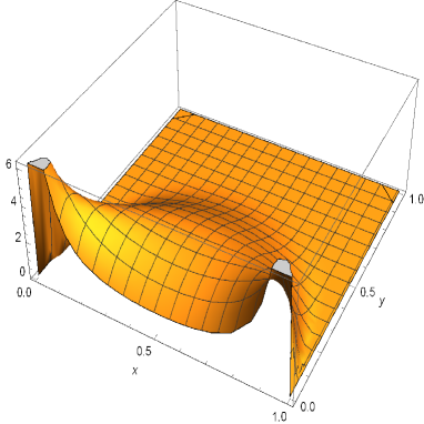
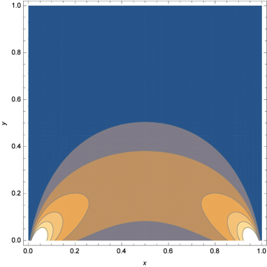
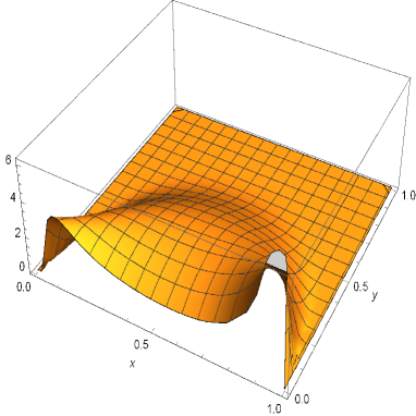
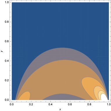
Figure 3: The 3D plot (left panel) and the corresponding 2D contour plot (right panel )for $\psi^{\cal P}_{3;\pi}(x,y)$ (upper panel) and $\psi^{\cal P}_{3;K}(x,y)$ (lower panel) obtained from the linear parameters. In 2D contour plot, darker the regions are, smaller the wave functions are.

From the point of view of QCD, the quark DAs of a hadron depend on the scale $\mu$ which separates nonperturbative and perturbative regimes. In our LFQM, we can associate $\mu$ with the transverse integration cutoff via $|{\bf k}_{\perp}|\leq\mu$, which is the usual way how the normalization scale is defined for the LF wave function (see, e.g. Ref. BL80 ). In order to estimate this cutoff value, we made a 3-dimensional plot for the LF wave function $\psi^{\cal P}_{3;\pi(K)}(x,{\bf k}_{\perp})$ in the form of $\psi^{\cal P}_{3;\pi(K)}(x,y)$ by changing the variable ${\bf k}^{2}_{\perp}=y/(1-y)$ so that $y$ ranges from 0 to 1. Fig. 3 shows the 3D plot (left panel) and the corresponding 2D contour plot (right panel) for $\psi^{\cal P}_{3;\pi}(x,y)$ (upper panel) and $\psi^{\cal P}_{3;K}(x,y)$ (lower panel) that we obtain with the linear parameters listed in Table 1. We note that we assign the momentum fraction $x$ for $s$-quark and $(1-x)$ for the light $u(d)$-quark for $K$ meson case. In fact, we obtain the twist-3 quark DAs by performing the transverse integration up to infinity (or equivalently $y$ up to 1) without loss of accuracy due the presence of Gaussian damping factor. However, as one can see from the contour plots in Fig. 3, only the range of $0\leq y\leq 0.47$ contribute to the integral for both $\pi$ and $K$ meson cases. This implies that our cutoff scale corresponds to $y\simeq 0.47$ or equivalently $\mu\simeq|{\bf k}_{\perp}|\simeq 1$ GeV for the calculation of the twist-3 $\pi$ and $K$ meson DAs. Since the twist-2 quark DAs for $\pi$ and $K$ mesons were given in our previous work CJ_DA , we do not show them in this work again but note that the scale $\mu$ for the twist-2 DA is slightly smaller than that for the twist-3 DA. Considering both twist-2 and twist-3 DAs of $\pi$ and $K$ mesons, our numerical results show the range of scale $\mu$ as $0.75\leq\mu\leq 1$ GeV.

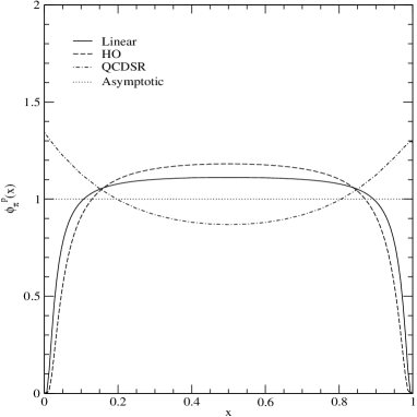
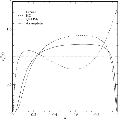
Figure 4: The twist-3 DAs $\phi^{\cal P}_{3;M}(x)$ for $\pi$ (left panel) and $K$ (right panel) mesons obtained from the linear (solid line) and HO (dashed line) parameters compared with the QCD sum rule result (dot-dashed line) BBL as well as the asymptotic one (dotted line) BF .

We show in Fig. 4 the twist-3 DAs $\phi^{\cal P}_{3;M}(x)$ [see Eq. (40)] for $\pi$ (left panel) and $K$ (right panel) mesons obtained from the linear (solid line) and HO (dashed line) parameters. We should note that our LFQM results $\phi^{\cal P}_{3;M}(x)$ are free from the explicit instantaneous as well as zero-mode contributions. The corresponding twist-2 DAs $\phi^{\cal A}_{2;M}$ for $(\pi,K)$ mesons obtained from our LFQM can be found in CJ_DA . We also compare our results with the the asymptotic DA $[\phi^{\cal P}_{3;M}]_{\rm as}(x)=1$ (dotted line) BF as well as the QCD sum-rule (QCDSR) prediction (dot-dashed line) BBL , which were obtained at the renormalization scale $\mu=1$ GeV. For the pion case, our results obtained from both model parameters not only show the symmetric forms anticipated from the isospin symmetry but also reproduce the exact asymptotic result $[\phi^{\cal P}_{3;\pi}]_{\rm as}(x)=1$ in the chiral symmetry ($m_{q}\to 0$) limit. This exact asymptotic result $\phi^{\cal P}_{3;\pi}(x)\to[\phi^{\cal P}_{3;\pi}]_{\rm as}(x)$ in the chiral symmetry limit is consistent with the conclusion drawn from our previous analysis CJ_V14 of the twist-2 ($\phi^{||}_{2;\rho}(x)$) and twist-3 ($\phi^{\perp}_{3;\rho}(x)$) $\rho$ meson DAs. Remarkably, both DAs reproduce the exact asymptotic DAs in the chiral symmetry limit. This example shows again that our LFQM prediction satisfies the chiral symmetry consistent with the QCD as one correctly implements the zero-mode link to the QCD vacuum. It is also interesting to note that while our results of $\phi^{\cal P}_{3;\pi}(x)$ become zero at the end points of $x$ unless the asymptotic limit is taken, while the QCD sum-rule result of Ref. BBL does not vanish at the end points. The main reason for the discrepancy between the two models is that the QCD sum-rule results are based on the chiral symmetry($m=0$) limit but our results (unless asymptotic) are based on the nonvanishing constituent quark model. In the asymptotic limit, our results exhibit also the nonvanishing behavior at the end points of $x$. For the $K$ meson case, $\phi^{\cal P}_{3;K}(x)$ obtained from both model parameters are asymmetric due to the flavor SU(3) symmetry breaking effect and the peak points located to the right of $x=0.5$ indicate that the $s$-quark carries more longitudinal momentum fraction than the light $u(d)$-quark.

The twist-2 and twist-3 quark DAs are usually expanded in terms of the Gegenbauer polynomials $C^{3/2}_{n}$ and $C^{1/2}_{n}$, respectively:

$$\phi^{\cal A}_{2;M} = [\phi^{\cal A}_{2;M}]_{\rm as}(x)\biggl{[}1+\sum^{\infty}_{n=1}a^{\cal A}_{n,M}C^{3/2}_{n}(2x-1)\biggr{]},$$

$$\phi^{\cal P}_{3;M} = [\phi^{\cal P}_{3;M}]_{\rm as}(x)\biggl{[}1+\sum^{\infty}_{n=1}a^{\cal P}_{n,M}C^{1/2}_{n}(2x-1)\biggr{]},$$ (45)

where $[\phi^{\cal A}_{2;M}]_{\rm as}(x)=6x(1-x)$ and $[\phi^{\cal P}_{3;M}]_{\rm as}(x)=1$. The coefficients $a^{\cal A(P)}_{n,M}$ are called the Gegenbauer moments and can be obtained from NK06

$$a^{\cal A}_{n,M}(x) = \frac{4n+6}{3n^{2}+9n+6}\int^{1}_{0}dx\;C^{3/2}_{n}(2x-1)\phi^{\cal A}_{2;M}(x),$$

$$a^{\cal P}_{n,M}(x) = (2n+1)\int^{1}_{0}dx\;C^{1/2}_{n}(2x-1)\phi^{\cal P}_{3;M}(x).$$ (46)

The Gegenbauer moments with $n>0$ describe how much the DAs deviate from the asymptotic one. In addition to the Gegenbauer moments, we can also define the expectation value of the longitudinal momentum, so-called $\xi(=2x-1)$-moments, as follows:

$$\langle\xi^{n}\rangle^{\cal A(P)}_{M}=\int^{1}_{0}dx\;\xi^{n}\phi^{\cal A(P)}_{2(3);M}(x).$$ (47)

Table 2: The Gegenbauer moments and $\xi$ moments of twist-2 and twist-3 pion DAs obtained from the linear and HO potential models compared other model estimates.

Models	Twists	$a^{\cal A(P)}_{2,\pi}$	$a^{\cal A(P)}_{4,\pi}$	$a^{\cal A(P)}_{6,\pi}$	$\langle\xi^{2}\rangle^{\cal A(P)}_{\pi}$	$\langle\xi^{4}\rangle^{\cal A(P)}_{\pi}$	$\langle\xi^{6}\rangle^{\cal A(P)}_{\pi}$
HO	$\phi^{\cal A}_{2;\pi}$	0.0514	-0.0340	-0.0261	0.2176	0.0939	0.0508
	$\phi^{\cal P}_{3;\pi}$	-0.5816	-0.4110	-0.1725	0.2558	0.1231	0.0723
Linear	$\phi^{\cal A}_{2;\pi}$	0.1234	-0.0033	-0.0218	0.2423	0.1136	0.0658
	$\phi^{\cal P}_{3;\pi}$	-0.3979	-0.3739	-0.2500	0.2803	0.1450	0.0907
SR Ball99	$\phi^{\cal P}_{3;\pi}$	0.5158	0.2545	0.2162	$\cdots$	$\cdots$	$\cdots$
SR BBL	$\phi^{\cal P}_{3;\pi}$	0.4373	-0.0715	-0.1969	0.3865	0.2451	0.1788
SR HWZ04	$\phi^{\cal P}_{3;\pi}$	$\cdots$	$\cdots$	$\cdots$	$0.340\sim 0.359$	$0.164\sim 0211$	$\cdots$
SR HZW05	$\phi^{\cal P}_{3;\pi}$	$\cdots$	$\cdots$	$\cdots$	$0.52\pm 0.03$	$0.44\pm 0.01$	$\cdots$
$\chi$QM NK06	$\phi^{\cal P}_{3;\pi}$	-0.4307	-0.5559	-0.1784	0.2759	0.1367	0.0816

In Table 2, we list the calculated Gegenbauer moments and $\xi$ moments of twist-2 and twist-3 pion DAs obtained from the linear and HO potential models at the aforementioned scale $\mu\sim 1$ GeV. Although the results of twist-2 pion DA were listed in our previous work CJ_DA , we list them here again by increasing the significant figures for completeness of this work. We also compare our results of twist-3 DAs with other model estimates calculated at the scale $\mu=1$ GeV, e.g. QCD sum-rules Ball99 ; BBL ; HWZ04 ; HZW05 and the chiral quark model ($\chi$QM) NK06 . As expected from the isospin symmetry, all the odd Gegenbauer and $\xi$ moments vanish. It is interesting to note within our LFQM predictions that $a^{\cal P}_{2,\pi}$ of the twist-3 DA are negative while the second Gegenbauer moments $a^{\cal A}_{2,\pi}$ of the twist-2 DA are positive, regardless of the linear or the HO model parameters. Compared to other models for the twist-3 case, our results are quite different from those of QCD sum-rules Ball99 ; BBL ; HWZ04 ; HZW05 but consistent with the chiral quark model predictions NK06 . Again, the differences between our LFQM and QCD sum-rule may be attributed to different treatment of constituent quark masses as we discussed about the results shown in Fig. 4.

Table 3: The Gegenbauer moments and $\xi$ moments of twist-2 and twist-3 $K$ meson DAs obtained from the linear and HO potential models compared other model estimates.

Models	Twists	$a^{\cal A(P)}_{1,K}$	$a^{\cal A(P)}_{2,K}$	$a^{\cal A(P)}_{3,K}$	$a^{\cal A(P)}_{4,K}$	$a^{\cal A(P)}_{5,K}$	$a^{\cal A(P)}_{6,K}$
HO	$\phi^{\cal A}_{2;K}$	0.1316	-0.0278	0.0381	-0.0335	-0.0112	-0.0122
	$\phi^{\cal P}_{3;K}$	0.3187	-0.7800	-0.0647	-0.2923	-0.2223	-0.0396
Linear	$\phi^{\cal A}_{2;K}$	0.0894	0.0275	0.0575	-0.0243	0.0069	-0.0142
	$\phi^{\cal P}_{3;K}$	0.2662	-0.6104	0.0486	-0.3361	-0.1454	-0.1161
SR Ball99	$\phi^{\cal P}_{3;K}$	$\cdots$	0.2631	$\cdots$	-0.0522	$\cdots$	0.1470
SR BBL	$\phi^{\cal P}_{3;K}$	0.1837	0.2707	0.3953	-0.2469	0.0550	-0.2436
$\chi$QM NK06	$\phi^{\cal P}_{3;K}$	0.0236	-0.6468	-0.0367	-0.3724	-0.0200	-0.0940
Models	Twists	$\langle\xi^{1}\rangle^{\cal A(P)}_{K}$	$\langle\xi^{2}\rangle^{\cal A(P)}_{K}$	$\langle\xi^{3}\rangle^{\cal A(P)}_{K}$	$\langle\xi^{4}\rangle^{\cal A(P)}_{K}$	$\langle\xi^{5}\rangle^{\cal A(P)}_{K}$	$\langle\xi^{6}\rangle^{\cal A(P)}_{K}$
HO	$\phi^{\cal A}_{2;K}$	0.0790	0.1905	0.0411	0.0759	0.0248	0.0389
	$\phi^{\cal P}_{3;K}$	0.1062	0.2293	0.0600	0.1034	0.0389	0.0582
Linear	$\phi^{\cal A}_{2;K}$	0.0536	0.2094	0.0339	0.0895	0.0231	0.0486
	$\phi^{\cal P}_{3;K}$	0.0887	0.2519	0.0560	0.1217	0.0394	0.0725
SR BBL	$\phi^{\cal P}_{3;K}$	0.0612	0.3676	0.0593	0.2236	0.0520	$\cdots$
SR HZW05	$\phi^{\cal P}_{3;K}$	$-0.10\pm 0.03$	$0.43\pm 0.04$	$\cdots$	$\cdots$	$\cdots$	$\cdots$
$\chi$QM NK06	$\phi^{\cal P}_{3;K}$	0.0079	0.2471	0.0026	0.1166	0.0008	$\cdots$

In Table 3, we display the calculated Gegenbauer moments and $\xi$ moments of twist-2 and twist-3 $K$ meson DAs obtained from the linear and HO potential models and compare them with other model predictions. For the kaon case, the odd moments are nonzero due to the flavor SU(3) symmetry breaking and the first moments $a^{\cal A(P)}_{1,K}$ is proportional to the difference between the longitudinal momenta of the strange and nonstrange quarks in the two-particle Fock component. We note within our LFQM predictions that the SU(3) symmetry breaking effects are rather significant for the twist-3 DA than for the twist-2 DA CJ_DA . Our results for the twist-3 $\phi^{\cal P}_{3;K}$ are overall in good agreement with those of the $\chi$QM NK06 except the values of the first moment $a^{\cal P}_{1,K}$ and $\langle\xi^{1}\rangle^{\cal P}_{K}$ with an order-of-magnitude difference between the two models, which may be understandable because the degree of SU(3) symmetry breaking in $\chi$QM NK06 is rather small compare to our LFQM prediction. The shape of $\phi^{\cal P}_{3;K}$ obtained from $\chi$QM NK06 is very close to the symmetric and flat shape while the corresponding result from our LFQM has a rather sizable asymmetric form.

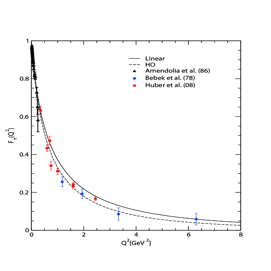
Figure 5: Pion electromagnetic form factors obtained from $F^{\rm SLF(+)}_{\pi}=[F_{\pi}]^{\rm SLF(\perp)}_{\rm on}$ using the linear (solid line) and HO (dashed line) potential models.

In Fig. 5, we show our numerical results of the pion electromagnetic form factor from $F^{\rm SLF(+)}_{\pi}=[F_{\pi}]^{\rm SLF(\perp)}_{\rm on}$ using the linear (solid line) and HO (dashed line) potential parameters and compare with the available experimental data Am86 ; Be78 ; Hu08 up to the $Q^{2}\sim 8$ GeV² region. In our previous LFQM analysis of the pion form factor CJ06 ; CJ08 , we have also shown that the usual power-law behavior of the pion form factor obtained in the perturbative QCD analysis can also be attained by taking negligible quark masses in our nonperturbative LFQM, confirming the anti-de Sitter space geometry/conformal field theory (AdS/CFT) correspondence BT04 .

V Summary and Discussion

As the zero-mode contribution is locked into a single point of the LF longitudinal momentum in the meson decay process, one of the constituents of the meson carries the entire momentum of the meson and it is important to capture the effect from a pair creation of particles with zero LF longitudinal momenta from the strongly interacting vacuum. The LFQM with effective degrees of freedom represented by the constituent quark and antiquark may thus provide the view of effective zero-mode cloud around the quark and antiquark inside the meson. Consequently, the constituents dressed by the zero-mode cloud may be expected to satisfy the chiral symmetry of QCD. Our results of this work for pseudoscalar mesons and the previous work for vector mesons were consistent with this expectation and effectively indicated that the constituent quark and antiquark in the standard LFQM could be considered as the dressed constituents including the zero-mode quantum fluctuations from the QCD vacuum.

In particular, we have discussed a wave function dependence of the LF zero-mode contributions to the twist-3 two-particle DA $\phi^{\cal P}_{3;M}$ of a pseudoscalar meson between the two models, i.e. the exactly solvable manifestly covariant BS model and the more phenomenologically accessible realistic LFQM using the the standard LF (SLF) approach following our previous work CJ_V14 . As the SLF approach within the LFQM by itself is not amenable to determine the zero-mode contribution, we utilized the covariant BS model to check the existence (or absence) of the zero-mode. Performing a LF calculation in the covariant BS model using the multipole type $q{\bar{q}}$ bound state vertex function, we found that the twist-3 $\phi^{\cal P}_{3;M}$ receives both the zero-mode and the instantaneous contributions and identified the zero-mode operator corresponding to the zero-mode contribution. We then linked the covariant BS model to the standard LFQM following the same correspondence relation Eq. (35) between the two models that we found in the vector meson decay amplitude CJ_V14 and substituted the LF vertex function in the covariant BS model with the more phenomenologically accessible Gaussian wave function provided by the LFQM analysis of meson mass CJ_99 . The remarkable finding is that the zero-mode contribution as well as the instantaneous contribution revealed in the covariant BS model become absent in the LFQM with the Gaussian wave function. Without engaging any of those treacherous contributions, our LFQM result of twist-3 DA $\phi^{\cal P}_{3;M}$ not only satisfies the fundamental constraint (i.e. symmetric form with respect to $x$) anticipated from the isospin symmetry but also provides the consistency with the chiral symmetry (e.g. the correct asymptotic form in the chiral symmetry limit) expected from the QCD. This observation commensurates our previous observation made in the analysis of vector meson decay process CJ_V14 .

We have also shown that our treatment of the treacherous points in two-point function is directly applicable to the three-point function, analyzing the pion elastic form factor $F_{\pi}(Q^{2})$ in the $q^{+}=0$ frame both with the plus component ($J^{+}_{\rm em}$) and the perpendicular component ($J^{\perp}_{\rm em}$) of the current. This analysis portrayed that the instantaneous contribution appeared in the covariant BS model became absent in the LFQM. It supports the conclusion drawn from the analysis of the two-point function.

From the self-consistent covariant description of the twist-3 $\phi^{\cal P}_{3;M}$ together with the previously obtained CJ_DA twist-2 DA $\phi^{\cal A}_{2;M}$ of a pseudoscalar meson in our LFQM, we presented a good deal of numerical results obtained from our LFQM. The quark condensate obtained from the normalization condition of $\phi^{\cal P}_{3;\pi}$, i.e. $\langle{\bar{q}}q\rangle=-(285.8{\rm MeV})^{3}[-(263.7{\rm MeV})^{3}]$ for the linear [HO] potential parameters comes out reasonable compared to the commonly used phenomenological value $-(250{\rm MeV})^{3}$. The ratio of the second transverse moments for the axial-vector and the pseudoscalar channels, $\langle{\bf k}^{2}_{\perp}\rangle^{\cal A}_{\pi}/\langle{\bf k}^{2}_{\perp}\rangle^{\cal P}_{\pi}=0.558~{}[0.597]$ for the linear [HO] parameters, is in good agreement with the QCD sum-rule result, 5/9 SR_C1 . Of particular interest, the mixed quark-gluon condensate of dimension 5 estimated from the value of $\langle{\bf k}^{2}_{\perp}\rangle^{\cal P}_{\pi}$ [see Eq. (44)], $\langle ig\bar{q}\sigma\cdot Gq\rangle=-(491.1~{}{\rm MeV})^{5}~{}[-(442.2~{}{\rm MeV})^{5}]$ for the linear [HO] parameters, is also in good agreement with the result $-(490~{}{\rm MeV})^{5}$ of the direct calculation in the instanton model PW . Moreover, our numerical results of $\phi^{\cal P}_{3;\pi}$ not only show the symmetric forms anticipated from the isospin symmetry but also reproduce the exact asymptotic result $[\phi^{\cal P}_{3;\pi}]_{\rm as}(x)=1$ in the chiral symmetry ($m_{q}\to 0$) limit. For the kaon case, the results of $\phi^{\cal P}_{3;K}$ show asymmetric form as expected from the flavor SU(3) symmetry breaking. Our results for the Gegenbauer moments and $\xi$ moments of twist-3 pion and kaon DAs are overall in good agreement with the chiral quark model NK06 although they differ from those of QCD sum-rule estimates Ball99 ; BBL ; HZW05 .

For further analysis, it would be interesting to study this process with other vertex function such as the symmetric product ansatz suggested in Eq. (38) of Ref. FPPS . The generalization of our findings to the three-point function would also require the analysis of unequal quark and antiquark mass cases.

- (1) G.P. Lepage and S.J. Brodsky, Phys. Rev. D 22, 2157 (1980).
- (2) A.V. Efremov and A.V. Radyushkin, Phys. Lett. B 94, 245 (1980).
- (3) V.L. Chernyak and A.R. Zhitnitsky, Phys. Rep. 112, 173 (1984).
- (4) V. M. Braun and I.E. Filyanov, Z. Phys. C 48, 239 (1990).
- (5) P. Ball, J. High Energy Phys. 01, 010 (1999).
- (6) P. Ball, V. M. Braun, and A. Lenz, J. High Energy Phys. 05, 004 (2006).
- (7) H.-M. Choi and C.-R. Ji, Phys. Rev. D 75, 034019 (2007).
- (8) M. Praszalowicz and A. Rostworowski, Phys. Rev. D 66, 054002 (2002).
- (9) S.I. Nam and H.-Ch. Kim, Phys. Rev. D 74, 096007 (2006).
- (10) T. Huang, X.H. Wu, and M.Z. Zhou, Phys. Rev. D 70, 014013 (2004).
- (11) T. Huang, M.Z. Zhou, and X.H. Wu, Eur. Phys. J. C 42, 271 (2005).
- (12) S. J. Brodsky, H. -C. Pauli, and S. Pinsky, Phys. Rep. 301, 299 (1998).
- (13) S. J. Brodsky and D. S. Hwang, Nucl. Phys. B 543, 239 (1999).
- (14) J.P.B.C. de Melo, J.H.O. Sales, T. Frederico, and P.U. Sauer, Nucl. Phys. A 631, 574c (1998).
- (15) H.-M. Choi and C.-R. Ji, Phys. Rev. D 58, 071901(R) (1998).
- (16) H.-M. Choi and C.-R. Ji, Phys. Rev. D 59, 074015 (1999); Phys. Lett. B 460, 461 (1999).
- (17) H.-M. Choi and C.-R. Ji, Phys. Rev. D 80, 054016 (2009).
- (18) W. Jaus, Phys. Rev. D 60, 054026 (1999).
- (19) W. Jaus, Phys. Rev. D 67, 094010 (2003).
- (20) H.-Y. Cheng, C.-K. Chua, and C.-W. Hwang, Phys. Rev. D 69, 074025 (2004).
- (21) H.-M. Choi and C.-R. Ji, Nucl. Phys. A 856, 95 (2011); Phys. Lett. B 696, 518 (2011).
- (22) J.P.B.C. de Melo and T. Frederico, Phys. Lett. B 708, 87 (2012).
- (23) W. Jaus, Phys. Rev. D 41, 3394 (1990).
- (24) H.-M. Choi, Phys. Rev. D 75, 073016 (2007).
- (25) H.-M. Choi and C.-R. Ji, Phys. Rev. D 89, 033011 (2014).
- (26) B.L.G. Bakker, M.A. DeWitt, C-R. Ji and Y. Mishchenko, Phys. Rev. D 72, 076005 (2005).
- (27) C.-R. Ji, W. Melnitchouk and A.W. Thomas, Phys. Rev. Lett. 110, 179101 (2013).
- (28) L. A. Kondratyuk and D. V. Tchekin, Physics of Atomic Nuclei 64, 727 (2001).
- (29) H.-Y. Cheng, C.-Y. Cheung, and C.-W. Hwang, Phys. Rev. D 55, 1559 (1997).
- (30) C.-W. Hwang, Phys. Rev. D 81, 114024 (2010).
- (31) W. Jaus, Phys. Rev. D 44, 2851 (1991).
- (32) P. L. Chung, F. Coester, and W. N. Polyzou, Phys. Lett. B 205, 545 (1988).
- (33) F. Cardarelli, I.L. Grach, I.M. Narodetskii, G. Salme, S. Simula, Phys. Lett. B 349, 393 (1995).
- (34) H.-M. Choi, C.-R. Ji, and L.S. Kisslinger, Phys. Rev. D 65, 074032 (2002).
- (35) M. Gell-Mann, R. Oakes, and B. Renner, Phys. Rev. 175, 2195 (1968).
- (36) B.L.G. Bakker, H.-M. Choi, and C.-R. Ji, Phys. Rev. D 63, 074014 (2001).
- (37) L.S. Kisslinger, H.-M. Choi, and C.-R. Ji, Phys. Rev. D 63, 113005 (2001).
- (38) H.-M. Choi and C.-R. Ji, Phys. Rev. D 74, 093010 (2006).
- (39) H.-M. Choi and C.-R. Ji, Phys. Rev. D 77, 113004 (2008).
- (40) S.J. Brodsky and Guy F. de Teramond, Phys. Lett. B 582, 211 (2004); Phys. Rev. Lett. 96, 201601 (2006).
- (41) J.P.B.C. de Melo and T. Frederico, Phys. Rev. C 55, 2043 (1997).
- (42) C.M. Shakin and W.-D. Sun, Phys. Rev. C 51, 2171 (1995).
- (43) J.P.B.C. de Melo, T. Frederico, E.Pace, and G. Salmé, Nucl. Phys. A 707, 399 (2002).
- (44) B.L.G. Bakker, H.-M. Choi, and C.-R. Ji, Phys. Rev. D 67, 113007 (2003).
- (45) H. J. Melosh, Phys. Rev. D 9, 1095 (1974); P. L. Chung, F. Coester, B. D. Keister, and W. N. Polyzou, Phys. Rev. C 37, 2000 (1988).
- (46) K.A. Olive et al. (Particle Data Group), Chin. Phys. C 38, 090001 (2014).
- (47) V.L. Chernyak, A.R. Zhitnitsky, and I.R. Zhitnitsky, Yad. Fiz. 38, 1074 (1983) [Sov. J. Nucl. Phys. 38, 645 (1983)].
- (48) A.R. Zhitnitsky, Phys. Lett. B 329, 493 (1994).
- (49) M.V. Polyakov and C. Weiss, Phys. Lett. B 387, 841 (1996).
- (50) S. R. Amendolia et al., Nucl. Phys. B 277, 168 (1986).
- (51) C. J. Bebek et al., Phys. Rev. D 17, 1693 (1978).
- (52) C. M. Huber et al., Phys. Rev. C 78, 045203 (2008).
- (53) T. Frederico, E. Pace, B. Pasquini, and G. Salme, Phys. Rev. D 80, 054021 (2009).