Projection of the low-lying eigenmodes of the overlap Dirac operator in lattice QCD

Abstract:

We outline our implementation of the adaptive thick-restart Lanczos algorithm ($a$-TRLan) for the projection of the low-lying eigenmodes of the overlap Dirac operator in lattice QCD, and compare the performances of our code and the widely used package ARPACK.

1 Introduction

To compute all eigenmodes of a large sparse matrix is a very challenging problem. However, for most studies, only a small subset of the entire spectrum plays the dominant role. Thus it is feasible to use an iterative algorithm to project this subset of eigenmodes.

In lattice QCD, it is well-known that the low-lying eigenmodes $(\lambda_{i},q_{i})$ of the Hermitian Dirac operator $H$ (where $H=\gamma_{5}D$, and $D$ is the Dirac operator which satisfies the $\gamma_{5}$-Hermiticity, $D^{\dagger}=\gamma_{5}D\gamma_{5}$) can serve as a basis to tackle many problems. For example, to compute the quark propagator $x=D^{-1}b$, it amounts to solving the linear system $H^{2}x=D^{\dagger}b\equiv c$ with the conjugate gradient algorithm (CG). Since the convergence rate of CG is proportional to the condition number $\lambda_{\mathrm{max}}^{2}/\lambda_{\mathrm{min}}^{2}$ (where $\lambda_{\mathrm{max}}/\lambda_{\mathrm{min}}$ are the largest/smallest eigenvalues of $|H|$), the convergence can be accelerated with the low-mode preconditioning. With the projected low modes $(\lambda_{i},q_{i})$ of $H^{2}$, CG can be performed in the orthogonal complement of the subspace spanned by the low modes, i.e.,

$$H^{2}\tilde{x}=\left(I-\sum_{i}q_{i}q_{i}^{\dagger}\right)c,$$

and the final solution is

$$x=\tilde{x}+\sum_{i}\frac{1}{\lambda_{i}^{2}}q_{i}q_{i}^{\dagger}c.$$

Another application of the low-lying eigenmodes (of the Wilson-Dirac operator) is to obtain a better approximation (chiral symmetry) of the overlap-Dirac operator $D_{\mathrm{ov}}$ for massless fermion [1]

$$D_{\mathrm{ov}}=m_{0}\left[1+\gamma_{5}\,\mathrm{sgn}(H_{w})\right],\hskip 11.38109pt{\rm sgn}(H_{w})=\frac{H_{w}}{\sqrt{H_{w}^{2}}},$$ (1)

where $H_{w}$ is the Hermitian Wilson-Dirac operator plus a negative parameter $-m_{0}$ ($0<m_{0}<2$). Since $(H_{w}^{2})^{-1/2}$ cannot be evaluated exactly, one often uses the Zolotarev optimal rational approximation [2]. For a given order of the optimal rational polynomial $R_{Z}(H_{w}^{2})$, it attains the optimal approximation of $(H_{w}^{2})^{-1/2}$ in the interval $[\lambda_{\mathrm{min}}^{2},\lambda_{\mathrm{max}}^{2}]$ of the spectrum of $H_{w}^{2}$. Moreover, for a given order, a smaller ratio $(\lambda_{\mathrm{max}}^{2}/\lambda_{\mathrm{min}}^{2})$ gives a better approximation. Thus, with the projected low modes of $H_{w}^{2}$, the matrix-vector product ($D_{\rm ov}v$) can be decomposed into the low-mode and the high-mode parts as

$$D_{\mathrm{ov}}v=m_{0}\biggl{\{}1+\gamma_{5}\sum_{i}q_{i}\,\mathrm{sgn}(\lambda_{i})q_{i}^{\dagger}+\gamma_{5}\,H_{w}R_{Z}(H_{w}^{2})\Bigl{(}I-\sum_{i}q_{i}q_{i}^{\dagger}\Bigr{)}\biggr{\}}v,$$ (2)

which yields better chiral symmetry than those without low modes.

The physical significances of the low-modes of the overlap Dirac operator are related to the topological quantum fluctuations of the QCD vacuum. According to the Atiyah-Singer index theorem [3], the numbers of zero modes ($n_{\pm}$) of the overlap Dirac operator provide an unambiguous determination of the topological charge ($Q_{t}$) of the gauge background,

$$Q_{t}\equiv\int d^{4}x\,\rho_{Q}(x)=n_{+}-n_{-}=\mathrm{index}(D_{\rm ov}),$$ (3)

where $\rho_{Q}(x)$ is the topological charge density, and $n_{\pm}$ is the number of zero modes of $D_{\rm ov}$ with $\pm$ chirality. Then we can also obtain the topological susceptibility,

$$\chi_{t}=\int d^{4}x\{\rho_{Q}(x)\rho_{Q}(0)\}=\frac{\left<Q_{t}^{2}\right>}{\Omega},$$ (4)

which can be used to determine the low-energy constants (e.g., $\Sigma$, $F_{\pi}$) through the chiral perturbation theory (ChPT) [4, 5]. Moreover, the spontaneous chiral symmetry breaking is related to the spectrum of the low-lying modes near $\lambda=0$, as depicted by the Banks-Casher relation [6]

$$\Sigma=-\langle\bar{\psi}\psi\rangle=\pi\rho(0),$$ (5)

where $\rho(0)$ is the density of eigenvalues near $\lambda=0$.

In general, to project a subset of eigenmodes of a large sparse matrix $A$, the standard procedure is to construct a Krylov subspace of $A$ from a starting vector $r_{0}$,

$$\mathcal{K}(A,r_{0})=\left\{r_{0},\,Ar_{0},\,A^{2}r_{0},\,\ldots,\,A^{m-1}r_{0}\right\}.$$ (6)

Then an orthonormal basis of the $m$-dimensional subspace can be constructed, which are regarded as approximated eigenvectors of $A$, the Ritz vectors.

In general, the Arnoldi method [7, 8] is an efficent way to perform the “implicit shifted QR iteration” on the Krylov subspace during restarts, which has been implemented in the widely used package ARPACK. However, for Hermitian matrices, it is more advantageous to use the Lanczos algorithm [9] to obtain the orthonormal basis in the Krylov subspace. In lattice QCD, the objective is to obtain the low-lying eigenmodes of the positive-definite Hermitian matrix $H^{2}$, which has become a challenging large-scale computation. Thus it is crucial to develop highly efficient algorithms and paradigms, based on the Lanczos algorithm and its variants.

This paper is organized as follows. In section 2, we outline the underlying theme for the projecton of the low-lying eigenmodes of the overlap Dirac operator in lattice QCD, and our implementation of the adaptive Thick-Restart Lanczos algorithms ($a$-TRLan). In section 3, we compare the performances of our code and the widely used ARPACK, and present our test results. Finally we conclude with some remarks.

2 Projection of the low-lying eigenmodes of the overlap-Dirac operator

In this section, we outline our scheme of projecting the low-lying eigenmodes of the overlap-Dirac operator $D_{\mathrm{ov}}$ (1) for massless fermion.

The eigenvalues of $D_{\mathrm{ov}}$ are lying on a circle in the complex plane with center at $(m_{0},0)$ and radius of length $m_{0}$, consisting of complex eigenmodes in conjugate pairs, and (for topologically nontrivial gauge background) real eigenmodes with eigenvalues at $0$ and $2m_{0}$ satisfying the chirality sum rule, $n_{+}-n_{-}+N_{+}-N_{-}=0$ [10], where $n_{\pm}(N_{\pm})$ denote the number of eigenmodes at $0$ ($2m_{0}$) with $\pm$ chirality. Empirically, the real eigenmodes always satisfy either ($n_{+}=N_{-}$, $n_{-}=N_{+}=0$) or ($n_{-}=N_{+}$, $n_{+}=N_{-}=0$). In other words, the zero modes only appear in either positive or negative chirality. Obviously, each eigenvector can be denoted by $\left|\theta\right>$, satisfying

$$D_{\mathrm{ov}}\left|\theta\right>=\lambda(\theta)\left|\theta\right>,\hskip 5.69054pt\lambda(\theta)=m_{0}(1+e^{i\theta}),\hskip 5.69054pt\theta\in[0,2\pi).$$ (7)

Using $[D_{\mathrm{ov}}D_{\mathrm{ov}}^{\dagger},\gamma_{5}]=0$, the eigenvector can be decomposed into positive and negative chiralities,

$$S_{\pm}\left|\theta\right>_{\pm}\equiv P_{\pm}S_{\mathrm{opt}}(H_{w})P_{\pm}\left|\theta\right>_{\pm}=P_{\pm}H_{w}R_{Z}(H_{w}^{2})P_{\pm}\left|\theta\right>_{\pm}=\pm\cos\theta\left|\theta\right>_{\pm},\quad$$ (8)

where $P_{\pm}=(1\pm\gamma_{5})/2$, $\left|\theta\right>_{\pm}=P_{\pm}\left|\theta\right>$. Moreover, for complex eigenmodes, $\left|\theta\right>_{+}$ and $\left|\theta\right>_{-}$ are related to each other through the relation

$$\left|\theta\right>=\frac{1}{i\sin\theta}(\gamma_{5}S_{\mathrm{opt}}-e^{-i\theta})\left|\theta\right>_{\pm},\hskip 28.45274pt\theta\neq 0,\pi.$$ (9)

Thus our strategy of projecting the low-lying modes of $D_{\rm ov}$ is as follows. First, we check whether the zero modes are in the positive or negative chirality sector. Then we project the low-lying eigenmodes in the same chirality sector of the zeromodes (if there are no zeromodes, just pick either one of the chiralty sectors), and finally obtain the eigenvectors of the complex eigenmodes using (9). To compute the matrix-vector product $R_{Z}(H_{w}^{2})\left|\theta\right>_{\pm}$ in (8) and (9), we use multi-shift CG with low-mode preconditioning and the two-pass algorithm [11, 12]. Therefore, we first project the low-lying eigenmodes of $H_{w}^{2}$, before doing the low-mode projection of (8). In both cases, we use the adaptive thick restart Lanczos algorithm ($a$-TRLan) [13, 14] for the low-mode projection.

In the following, we outline the basic ideas of $a$-TRLan. Consider a $N\times N$ Hermitian matrix $A$. After $m$ Lanczos iterations, it gives

$$AQ_{m}=Q_{m}T_{m}+\beta_{m}q_{m+1}e^{\dagger}_{m}$$ (10)

where $T_{m}$ is a $m\times m$ tridiagonal matrix, and $Q_{m}$ is the unitary matrix formed by the orthonormal vectors $\{q_{i},i=1,2,\ldots,m\}$ which are generated in the Lanczos iterations. The last term is called the residual, where $e_{m}$ is the unit vector with all elements zero except the $m$-th entry, and $\beta_{m}$ is the norm of the residual. After diagonalizing $T_{m}$, we obtain $m$ Ritz pairs, $\{(\lambda_{i},y_{i}):\lambda_{1}<\lambda_{2}<\cdots<\lambda_{m}\}$. Since the Ritz values first converge to the exterior eigenvalues of $A$, we select $k$ Ritz pairs from both ends for the restart, namely $i=1,\cdots,l,u,\cdots,m$, where $k=m+l-u+1$, and to perform re-orthogonalization if necessary. Then the Lanczos iterations are restarted for $k+1,\cdots,m$. The same procedures (diagonalization, truncation, re-orthogonalization, and restart) are repeated until the desired number of Ritz pairs are converged.

Theoretically, the subspace dimension $m$ and the number $k$ of selected Ritz pairs for the restart, i.e., the triplet $(l,u,m)$ can be tuned for each restart to optimize the overall performance, i.e., the convergent rate versus the computational time of each restart, based on the estimates from all previous iterations. This leads to the $a$-TRLan algorithm [14]. This amounts to maximizing the object function (i.e., the ratio of the convergence rate and the computation time) at each restart,

$$f(l,m,k)=\frac{\omega(m,k,\gamma)}{T(m,k)}\simeq\frac{2(m-k)\sqrt{\gamma}}{2t_{1}(m-k)(k+m-1)+2t_{2}mk+t_{3}(m-k)},$$ (11)

where $\omega$ measures the convergent rate of the smallest non-convergent Ritz value ($\lambda_{l+1}$), which can be estimated as $2(m-k)\sqrt{\gamma}$, with $\gamma=(\lambda_{l+2}-\lambda_{l+1})/(\lambda_{u-1}-\lambda_{l+2})$, the effective gap ratio. Here $t_{1},t_{2},t_{3}$ are average computation times (measured from all previous iterations) for reorthogonalization, computing Ritz vectors, and matrix-vector product respectively.

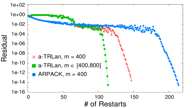
Figure 1: The residual of the last (the 250-th) Ritz pair of $H_{w}^{2}$ versus the number of restarts, for $a$-TRLan with fixed $m$, $a$-TRLan with tunable $m$, and ARPACK respectively. Here $m$ is the dimension of the Krylov subspace. For the $a$-TRLan cases (the red and green points), the relaxation parameter $\nu$ is set to 0.5.

According to our experience, taking $u=m+1$ is always the best choice. Thus we restrict our discussions to the case $k=l$. In our code, the variation of $m$ is limited to an interval [$m_{\mathrm{min}}$, $m_{\mathrm{max}}$], with the initial $m=m_{\rm min}$. Assuming the number of converged Ritz pairs is $n_{\mathrm{conv}}$, then $k$ is varied with the constraint $n_{\rm conv}+1\leq k\leq k_{0}<m$, where $k_{0}=m+1-\nu(m-n_{\mathrm{conv}})$, with $\nu$ the relaxation (input) parameter. At the $j$-th restart, after $m_{j}$ Lanczos iterations, and the diagonalization of the tridiagonal matrix $T_{m_{j}}$, the code searches for the optimal values of $(m_{j+1},k_{j+1})$ to maximize the object function (11) with the constraint $k_{j+1}<m_{j}$, which are then used for the $(j+1)$-th restart.

3 Performance Tests

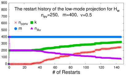
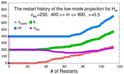
(a)	(b)

Figure 2: The restart history of projecting the low-modes of $H_{w}^{2}$ with the $a$-TRLan algorithm. Here $n_{\mathrm{ev}}$ is the number of desired eigenmodes, $m$ is the dimension of the Krylov subspace, $\nu$ is the relaxation factor. $k$ is the dimension at restart, $n_{\mathrm{conv}}$ is the number of converged Ritz pairs, and $n_{Av}$ is the number of matrix-vector multiplication between each restart. In (a) $m$ is fixed at 400, only $k$ is tunable during the restarts. In (b) both $(m,k)$ are tunable during the restarts, in which the range of $m$ is confined within $[400,800]$.

In this section, we perform some tests to compare the performances of our code and ARPACK. Our testing platform is a Supermicro server with dual Intel Xeon E5530 (2.40 GHz) CPU and 24 GB memory. There are totally 8 cores in the machine. Hence we run each of the tests with 8 threads in parallel.

In Fig. 1, we plot the convergence rate of the low-modes of $H_{w}^{2}$, for a typical configuration in the gauge ensemble obtained by the dynamical simulation of 2-flavors lattice QCD with optimal domain-wall quarks [15] on the $16^{3}\times 32$ lattice at $\beta=5.95$ and $m_{sea}a=0.01$ [16]. Here we compare the performances of three different schemes: (1) $a$-TRLan with fixed $m=400$, i.e., only tuning $k$. (2) $a$-TRLan with tunable $(m,k)$ for $m\in[400,800]$. (3) ARPACK with fixed $m=400$. In each case, we project 250 low-lying eigenmodes of $H_{w}^{2}$, and plot the residual of the last (the 250-th) Ritz pair versus the number of restarts. The stopping criteira is $10^{-13}$ for the residual of any Ritz pair. For $a$-TRLan, the relaxation factor $\nu$ is fixed at 0.5. Here we see that $a$-TRLan takes much less restarts than ARPACK. Furthermore, $a$-TRLan with tunable $(m,k)$ outperforms that with fixed $m$. The computation time for each case is given in Table 1.

In Fig. 2, we plot the history of restart corresponding to the low-mode projection in Fig. 1. In (a) the dimension of the Krylov subspace $m$ is fixed at 400, thus the optimization amounts to search for the optimal $k$ for the next restart. On the other hand, $m$ is not fixed in (b), thus the algorithm searches for the optimal values of $(m,k)$. Here we see that the value of $k$ increases monotonically with respect to the number of converged Ritz pairs $n_{\mathrm{conv}}$. In (a), since $m$ is fixed, the required Lanczos iterations after each restart (i.e., $m-k-1$) gets fewer and fewer. On the other hand, in the case of (b), $m$ and $k$ both increase monotonically with respect to $n_{\mathrm{conv}}$, the required Lanczos iterations for each restart is almost the same, but the required number of restarts is less than (a). Overall, (b) runs faster than (a) (see Table 1).

	$\nu=0.7$				$\nu=0.6$				$\nu=0.5$				ARPACK
$m$	$m_{M}$	$n_{R}$	$n_{Av}$	time	$m_{M}$	$n_{R}$	$n_{Av}$	time	$m_{M}$	$n_{R}$	$n_{Av}$	time	$n_{R}$	$n_{Av}$	time
300	300	361	33196	40095	300	346	28137	36799	300	361	33196	40095	1710	47728	163010
400	400	128	24433	30907	400	121	21502	26343	400	146	21569	29168	220	22255	56702
500	500	75	21466	30928	500	88	21526	30197	500	75	21466	31286	120	21571	57227
600	600	59	21445	32743	600	69	21468	33949	600	59	21445	32426	78	21262	59260
$[300,800]$	412	243	31419	30791	458	203	26143	26907	565	186	24064	24581	n/a	n/a	n/a
$[400,800]$	430	126	24387	21802	453	118	21510	25858	558	132	21546	23905	n/a	n/a	n/a
$[500,800]$	500	75	21466	30994	500	88	21526	30224	546	104	21478	29620	n/a	n/a	n/a
$[600,800]$	600	59	21445	32778	600	69	21468	34016	600	83	21499	32513	n/a	n/a	n/a

Table 1: Comparing performances of various schemes of $a$-TRLan and ARPACK, for the projection of low-modes of $H_{w}^{2}$. For $a$-TRLan, both fixed $m$ and tunable $m$ are considered for various settings of the relaxation factor $\nu=0.7$, 0.6, and 0.5. Here $m_{M}$ is the maximum dimension of the Krylov subspace in the projection, $n_{R}$ is the number of restarts to complete the job, $n_{Av}$ is the total number of matrix-vector multiplication, and the total computation time is in unit of second.

In Table 1, we compare the performance of projecting 250 low-lying eigenmodes of $H_{w}^{2}$ for the same gauge configuration presented in Fig. 1. For the $a$-TRLan algorithm, we also compare different settings of $\nu$ and $m$, with both cae of fixed $m$ and tunable $m$. Here we show how the setting of $m$ and $\nu$ affects the performance. For the cases with fixed $m$, it seems that setting $m$ at around 400 or 500 can attend a reasonably good performance for all the values of $\nu$, and setting $\nu=0.6$ seems to be the best choice. Now we compare the results of fixing $m=m_{\mathrm{min}}$ and tunable $m\in[m_{\mathrm{min}},800]$, where $m_{\mathrm{min}}=300$, 400, 500, and 600 are the lower bounds for the tuning $m$. We see that in some cases the maximum values of $m$ (i.e., $m_{M}$) during the projection may saturate. For example, at $\nu=0.7$, setting the lower bound $m_{\mathrm{min}}$ to 500 or 600, $m_{M}$ (for the tunable cases) remains constant during the entire projection. Thus, the restart histories of both fixed $m=m_{\mathrm{min}}$ and tunable $m\in[m_{\mathrm{min}},800]$ are exactly identical. On the other hand, if $m_{M}$ is not saturated, then those with tunable $m$ outperform their counterparts with fixed $m$. In the last three columns of Table 1, we list the performance of ARPACK for the same projection task. Here neither $m$ nor $k$ is tunable in ARPACK. Obviously, any scheme of $a$-TRLan in Table 1 outperforms ARPACK.

	$\nu=0.6$				$\nu=0.5$				$\nu=0.4$				ARPACK
$m$	$m_{M}$	$n_{R}$	$n_{Av}$	time	$m_{M}$	$n_{R}$	$n_{Av}$	time	$m_{M}$	$n_{R}$	$n_{Av}$	time	$n_{R}$	$n_{Av}$	time
300	300	13	2002	65657	300	15	1967	64754	300	19	1968	64744	27	1986	77613
400	400	8	2029	66827	400	9	1961	64619	400	12	2010	66249	12	1966	78014
500	500	6	2110	69561	500	7	2072	68479	500	6	1950	64730	8	2082	83368
600	600	4	2003	66130	600	5	2038	67498	600	6	1988	65884	5	1996	79350
$[300,800]$	524	9	2126	69799	597	8	2017	66454	759	7	2018	66580	n/a	n/a	n/a
$[400,800]$	460	7	1979	65134	535	7	1951	64260	685	7	2030	67240	n/a	n/a	n/a
$[500,800]$	532	6	2147	70828	589	6	2026	66835	651	6	1950	64729	n/a	n/a	n/a
$[600,800]$	600	4	2003	66238	627	5	2065	68286	817	5	2131	70770	n/a	n/a	n/a

Table 2: The performance comparison of low-mode projection for $S_{+}$ using the $a$-TRLan algorithm with fixed and tunable $m$, and for various settings of the relaxation factor $\nu=0.6$, 0.5, 0.4, together with the performance of ARPACK. Here $m_{M}$ is the maximum dimension of the Krylov subspace during the projection, $n_{R}$ is the number of restarts to complete the job, $n_{Av}$ is the total number of matrix-vector multiplication, and the running time is in unit of seconds.

Now, with 250 low-modes of $H_{w}^{2}$, we proceed to project the 200 low-modes of the overlap Dirac operator. For the matrix-vector product $R_{Z}(H_{w}^{2})\left|\theta\right>_{\pm}$ in (8) and (9), we use multi-shift CG with low-mode preconditioning and the two-pass algorithm [11, 12]. In Table 2, we present our test results of low-mode projection of $S_{+}$ (8) for the same gauge configuration. Note that $S_{\pm}\cdot v$ is a complicated matrix-vector operation since it involves two inner CG loops (for the two-pass algorithm) [11, 12], which takes much longer time than $H_{w}^{2}\cdot v$. For this configuration, the ratio of the computation times of these two matrix-vector multiplications is

$$\frac{T_{Av}(S_{+})}{T_{Av}(H_{w}^{2})}\simeq 1120.$$

Thus, for the low-mode projection of $S_{\pm}$, the computation time is dominated by the total number of matrix-vector multiplication $n_{Av}$. Consequently, $a$-TRLan with tunable $m$ is not necessarily faster than that with fixed $m$. Even though the object function is supposed to predict the optimal values of $(m,k)$, it does not guarantee to yield the smallest value of $n_{Av}$ which dominates the cost of the computation. This issue requires further studies which are beyond the scope of the present paper. From Table 2, setting $\nu=0.5$ and $m=400$ seems to give the best performance. From the last 3 columns in Table 2, we see that the performance of $a$-TRLan is only 20% to 30% better than ARPACK, unlike the case of $H_{w}^{2}$ (see Table 1). We believe that there is still room for improving the performance of the low-mode projection of $S_{\pm}$ with $a$-TRLan.

At this point, it is instructive to compare the overall performances of our $a$-TRLan code and ARPACK, for the projection of 200 low-lying modes of the overlap Dirac operator, including the time in the projection of 250 low-modes of $H_{w}^{2}$. Taking into account of the time (6550 seconds) used in evaluating (9), our results in Tables 1 and 2 suggest that our $a$-TRLan code is about 1.5 times faster than ARPACK. Moreover, if one is only interested in the projection of low-modes of the Wilson (clover) quark matrix, our results in Table 1 suggest that $a$-TRLan is more than 2 times faster than ARPACK.

4 Concluding remarks

In this work, we have implemented the $a$-TRLan algorithm to project the low-lying eigenmodes of the Dirac operators $H_{w}$ and $D_{\mathrm{ov}}$. Our code searches for the optimal values of $(m,k)$ at each restart to maximize the object function (11) which is the ratio of the convergence rate (of the smallest non-convergent Ritz value) and the computation time. For the low-mode projection of $H_{w}^{2}$, $a$-TRLan works very well and outpeforms ARPACK significantly. However, for the low-mode projection of $S_{\pm}$, $a$-TRLan with fixed $m$ is only about 20%-30% faster than ARPACK. Moreover, $a$-TRLan with tunable $(m,k)$ does not perform better than that with fixed $m$. To clarify this issue requires further studies which are now in progress.

To summarize, we find that $a$-TRLan is an efficient algorithm for the projection of low-modes of the quark matrix in lattice QCD. For the Wilson (clover) quark matrix, $a$-TRLan is more than 2 times faster than ARPACK. For lattice QCD with exact chiral symmetry, the projection of the low-modes of the quark matrix includes two different projections (i.e., those of $H_{w}^{2}$ and $S_{\pm}$). Currently, our $a$-TRLan code is about 1.5 times faster than ARPACK.

- [1] H. Neuberger, Phys. Lett. B 417, 141 (1998); [arXiv:hep-lat/9707022].
- [2] T. W. Chiu, T. H. Hsieh, C. H. Huang and T. R. Huang, Phys. Rev. D 66, 114502 (2002). [hep-lat/0206007].
- [3] M. F. Atiyah and I. M. Singer, Annals Math. 87, 484 (1968).
- [4] H. Leutwyler and A. V. Smilga, Phys. Rev. D 46 (1992) 5607.
- [5] Y.Y. Mao and T.W. Chiu [TWQCD Collaboration], Phys. Rev. D 80, 034502 (2009). [arXiv:0903.2146 [hep-lat]].
- [6] T. Banks and A. Casher, Nucl. Phys. B 169, 103 (1980).
- [7] W.E. Arnoldi, Quart. Appl. Math., 9 (1951) 17.
- [8] D.S. Sorensen, SIAM J. Matrix Anal. Appl., 13 (1992) 357.
- [9] C. Lanczos, J. Res. Nat. Bur. Std. 45, (1950) 225.
- [10] T. W. Chiu, Phys. Rev. D 58, 074511 (1998) [hep-lat/9804016].
- [11] H. Neuberger, Int. J. Mod. Phys. C 10, 1051 (1999) [hep-lat/9811019].
- [12] T. W. Chiu and T. H. Hsieh, Phys. Rev. E 68, 066704 (2003) [hep-lat/0306025].
- [13] K. Wu and H. Simon, SIAM J. Matrix Anal. Appl. 22 (2000) 602.
- [14] I. Yamazaki, Z. Bai, H. Simon, L.W. Wang, K. Wu, ACM Trans. Math. Software 37 (3) (2010) 27.
- [15] T. W. Chiu, Phys. Rev. Lett. 90, 071601 (2003) [arXiv:hep-lat/0209153].
- [16] T. W. Chiu, T. H. Hsieh and Y. Y. Mao [TWQCD Collaboration], Phys. Lett. B 717, 420 (2012) [arXiv:1109.3675 [hep-lat]].