Super-Resolution Compressed Sensing: A Generalized Iterative Reweighted $\ell_{2}$ Approach

Abstract

Conventional compressed sensing theory assumes signals have sparse representations in a known, finite dictionary. Nevertheless, in many practical applications such as direction-of-arrival (DOA) estimation and line spectral estimation, the sparsifying dictionary is usually characterized by a set of unknown parameters in a continuous domain. To apply the conventional compressed sensing technique to such applications, the continuous parameter space has to be discretized to a finite set of grid points, based on which a “presumed dictionary” is constructed for sparse signal recovery. Discretization, however, inevitably incurs errors since the true parameters do not necessarily lie on the discretized grid. This error, also referred to as grid mismatch, may lead to deteriorated recovery performance or even recovery failure. To address this issue, in this paper, we propose a generalized iterative reweighted $\ell_{2}$ method which jointly estimates the sparse signals and the unknown parameters associated with the true dictionary. The proposed algorithm is developed by iteratively decreasing a surrogate function majorizing a given objective function, resulting in a gradual and interweaved iterative process to refine the unknown parameters and the sparse signal. A simple yet effective scheme is developed for adaptively updating the regularization parameter that controls the tradeoff between the sparsity of the solution and the data fitting error. Extension of the proposed algorithm to the multiple measurement vector scenario is also considered. Numerical results show that the proposed algorithm achieves a super-resolution accuracy and presents superiority over other existing methods.

I Introduction

Compressed sensing finds a variety of applications in practice as many natural signals admit a sparse or an approximate sparse representation in a certain basis. Nevertheless, accurate reconstruction of a sparse signal relies on the knowledge of the sparsifying dictionary, while in many applications, it is often impractical to pre-specify a dictionary that can sparsely represent the signal. For example, for the line spectral estimation problem, using a preset discrete Fourier transform (DFT) matrix suffers from considerable performance degradation because the true frequency components may not lie on the pre-specified frequency grid [1, 2]. The same is true for direction-of-arrival (DOA) estimation and source localization in sensor networks, where the true directions or locations of sources may not be aligned on the presumed grid [3]. Overall, in these applications, the sparsifying dictionary is characterized by a set of unknown parameters in a continuous domain. In order to apply compressed sensing to such applications, the continuous parameter space has to be discretized to a finite set of grid points, based on which a presumed dictionary is constructed for sparse signal recovery. Discretization, however, inevitably incurs errors since the true parameters do not necessarily lie on the discretized grid. This error, also referred to as the grid mismatch, leads to deteriorated performance or even failure in recovering the sparse signal. Finer grids can certainly be used to reduce grid mismatch and improve the reconstruction accuracy. Nevertheless, recovery algorithms may become numerically instable and computationally prohibitive when very fine discretized grids are employed.

The grid mismatch problem has attracted a lot of attention over the past few years. Specifically, in [4], the problem was addressed in a general framework of “basis mismatch” where the mismatch is modeled as a perturbation (caused by grid discretization, calibration errors or other factors) between the presumed and the actual dictionaries, and the impact of the basis mismatch on the reconstruction error was analyzed. In [3, 5], to deal with grid mismatch, the true dictionary is approximated as a summation of a presumed dictionary and a structured parameterized matrix via the Taylor expansion. The recovery performance of this method, however, depends on the accuracy of the Taylor expansion in approximating the true dictionary. The grid mismatch problem was also examined in [6, 7], where a highly coherent dictionary (very fine grids) is used to mitigate the discretization error, and a class of greedy algorithms which use the technique of band exclusion (coherence-inhibiting) were proposed for sparse signal recovery. Besides these efforts, another line of work [8, 2, 1] studied the problem of grid mismatch in a more fundamental way: they circumvent the discretization issue by working directly on the continuous parameter space, leading to the so-called super-resolution technique. In [2, 1], an atomic norm-minimization (also referred to as the total variation norm-minimization) approach was proposed to handle the infinite dictionary with continuous atoms. It was shown that given that the frequency components are sufficiently separated, the frequency components of a mixture of complex sinusoids can be super-resolved with infinite precision from coarse-scale information only. Nevertheless, finding a solution to the atomic norm problem is quite challenging. Although the atomic norm problem can be cast into a convex semidefinite program optimization for the complex sinusoid mixture problem, it still remains unclear how this reformulation generalizes to other scenarios. In [8], by treating the sparse signal as hidden variables, a Bayesian approach was proposed to iteratively refine the dictionary, and is shown able to achieve super-resolution accuracy.

In this paper, we propose a generalized iterative reweighted $\ell_{2}$ method for joint dictionary parameter learning and sparse signal recovery. The proposed method is developed by iteratively decreasing a surrogate function that majorizes the original objective function. Note that the use of the iterative reweighted scheme for sparse signal recovery is not new and has achieved great success over past few years (e.g. [9, 10, 11, 12, 13]). Nevertheless, previous works concern only recovery of the sparse signal. The current work, instead, generalizes the iterative reweighted scheme for joint dictionary parameter learning and sparse signal recovery. Moreover, previous iterative reweighted algorithms usually involve iterative minimization of a surrogate function majorizing a given objective function, while our proposed method only requires iteratively decreasing a surrogate function. We will show that through iteratively decreasing (not necessarily minimizing) the surrogate function, the iterative process yields a non-increasing objective function value as well, and is guaranteed to converge to a stationary point of the objective function. This generalization extends the applicability of the iterative reweighted scheme since finding a simple and convex surrogate function which admits an analytical solution could be difficult for many complex problems. In addition, iteratively decreasing the surrogate function results in an interweaved and gradual refinement of the signal and the unknown parameters, which enables the algorithm to produce more focal and reliable estimates as the optimization progresses. The current work is an extension of our previous work [14] to more general scenarios involving noisy and/or multiple measurement vectors. As shown in this paper, this extension is technically non-trivial and also brings in substantial reduction in computational complexity.

The rest of the paper is organized as follows. In Section II, the line spectral estimation problem is formulated as a joint sparse representation and dictionary parameter estimation problem. A generalized iterative reweighted $\ell_{2}$ algorithm is developed in Section III. The choice of the regularization parameter controlling the tradeoff between sparsity and data fitting is discussed in Section IV, where a simple and effective update rule for the regularization parameter is proposed. Extension of the proposed algorithm to the multiple measurement vector scenario is studied in Section V. In Section VI, we provide a heuristic but enlightening analysis on the exact reconstruction condition of the considered problem for the noiseless case. Simulation results are provided in Section VII, followed by concluding remarks in Section VIII.

II Problem Formulation

In many practical applications such as direction-of-arrival (DOA) estimation and line spectral estimation, the sparsifying dictionary is usually characterized by a set of unknown parameters in a continuous domain. For example, consider the line spectral estimation problem where the observed signal is a summation of a number of complex sinusoids:

$$y_{m}=\sum_{k=1}^{K}\alpha_{k}e^{-j\omega_{k}m}+w_{m}\qquad m=1,\ldots,M$$ (1)

where $\omega_{k}\in[0,2\pi)$ and $\alpha_{k}$ denote the frequency and the complex amplitude of the $k$-th component, respectively, and $w_{m}$ represents the observation noise. Define $\boldsymbol{a}(\omega)\triangleq[e^{-j\omega}\phantom{0}e^{-j2\omega}\phantom{0}\ldots\phantom{0}e^{-jM\omega}]^{T}$, the model (1) can be rewritten in a vector-matrix form as

$$\boldsymbol{y}=\boldsymbol{A}(\boldsymbol{\omega})\boldsymbol{\alpha}+\boldsymbol{w}$$ (2)

where $\boldsymbol{y}\triangleq[y_{1}\phantom{0}\ldots\phantom{0}y_{M}]^{T}$, $\boldsymbol{\alpha}\triangleq[\alpha_{1}\phantom{0}\ldots\phantom{0}\alpha_{K}]^{T}$, and $\boldsymbol{A}(\boldsymbol{\omega})\triangleq[\boldsymbol{a}(\omega_{1})\phantom{0}\ldots\phantom{0}\boldsymbol{a}(\omega_{K})]$. Note that in some applications, to facilitate data acquisition and subsequent processing, we may wish to estimate $\{\omega_{k}\}$ and $\{\alpha_{k}\}$ from a subset of measurements randomly extracted from $\{y_{m}\}_{m=1}^{M}$. This random sampling operation amounts to retaining the corresponding rows of $\boldsymbol{A}(\boldsymbol{\omega})$ and removing the rest rows from the dictionary. This modification, however, makes no difference to our algorithm development.

We see that the dictionary $\boldsymbol{A}(\boldsymbol{\omega})$ is characterized by a number of unknown parameters $\{\omega_{k}\}$ which need to be estimated along with the unknown complex amplitudes $\{\alpha_{k}\}$. To deal with this problem, conventional compressed sensing techniques discretize the continuous parameter space into a finite set of grid points, assuming that the unknown frequency components $\{\omega_{k}\}$ lie on the discretized grid. Estimating $\{\omega_{k}\}$ and $\{\alpha_{k}\}$ can then be formulated as a sparse signal recovery problem $\boldsymbol{y}=\boldsymbol{Az}+\boldsymbol{w}$, where $\boldsymbol{A}\in\mathbb{C}^{M\times N}$ ($M\ll N$) is an overcomplete dictionary constructed based on the discretized grid points. Discretization, however, inevitably incurs errors since the true parameters do not necessarily lie on the discretized grid. This error, also referred to as the grid mismatch, leads to deteriorated performance or even failure in recovering the sparse signal.

To circumvent this issue, we treat the overcomplete dictionary as an unknown parameterized matrix $\boldsymbol{A}(\boldsymbol{\theta})\triangleq[\boldsymbol{a}(\theta_{1})\phantom{0}\ldots\phantom{0}\boldsymbol{a}(\theta_{N})]$, with each atom $\boldsymbol{a}(\theta_{n})$ determined by an unknown frequency parameter $\theta_{n}$. Estimating $\{\omega_{k}\}$ and $\{\alpha_{k}\}$ can still be formulated as a sparse signal recovery problem. Nevertheless, in this framework, the frequency parameters $\boldsymbol{\theta}\triangleq\{\theta_{n}\}_{n=1}^{N}$ need to be optimized along with the sparse signal such that the parametric dictionary will approach the true sparsifying dictionary. Specifically, the problem can be presented as follows: we search for a set of unknown parameters $\{\theta_{n}\}_{n=1}^{N}$ with which the observed signal $\boldsymbol{y}$ can be represented by as few atoms as possible with a specified error tolerance. Such a problem can be readily formulated as

$$\min_{\boldsymbol{z},\boldsymbol{\theta}}\quad \|\boldsymbol{z}\|_{0}$$

s.t. $$\|\boldsymbol{y}-\boldsymbol{A}(\boldsymbol{\theta})\boldsymbol{z}\|_{2}\leq\varepsilon$$ (3)

where $\|\boldsymbol{z}\|_{0}$ stands for the number of the nonzero components of $\boldsymbol{z}$, and $\varepsilon$ is an error tolerance parameter related to noise statistics. The optimization (3), however, is an NP-hard problem. Thus, alternative sparsity-promoting functionals which are more computationally efficient in finding the sparse solution are desirable. In this paper, we consider the use of the log-sum sparsity-encouraging functional for sparse signal recovery. Log-sum penalty function has been extensively used for sparse signal recovery, e.g. [15, 12]. It was proved theoretically [16] and shown in a series of experiments [11] that log-sum based methods present uniform superiority over the conventional $\ell_{1}$-type methods. Replacing the $\ell_{0}$-norm in (3) with the log-sum functional leads to

$$\min_{\boldsymbol{z},\boldsymbol{\theta}}\quad L(\boldsymbol{z})=\sum_{n=1}^{N}\log(|z_{n}|^{2}+\epsilon)\quad$$

s.t. $$\|\boldsymbol{y}-\boldsymbol{A}(\boldsymbol{\theta})\boldsymbol{z}\|_{2}\leq\varepsilon$$ (4)

where $z_{n}$ denotes the $n$th component of the vector $\boldsymbol{z}$, and $\epsilon>0$ is a positive parameter to ensure that the function is well-defined. The optimization (4) can be formulated as an unconstrained optimization problem by removing the constraint and adding a Tikhonov regularization term, $\lambda\|\boldsymbol{y}-\boldsymbol{A}(\boldsymbol{\theta})\boldsymbol{z}\|_{2}^{2}$, to the objective functional, which yields the following optimization

$$\min_{\boldsymbol{z},\boldsymbol{\theta}}\quad G(\boldsymbol{z},\boldsymbol{\theta})\triangleq \sum_{n=1}^{N}\log(|z_{n}|^{2}+\epsilon)+\lambda\|\boldsymbol{y}-\boldsymbol{A}(\boldsymbol{\theta})\boldsymbol{z}\|_{2}^{2}$$

$$= L(\boldsymbol{z})+\lambda\|\boldsymbol{y}-\boldsymbol{A}(\boldsymbol{\theta})\boldsymbol{z}\|_{2}^{2}$$ (5)

where $\lambda>0$ is a regularization parameter controlling the tradeoff between data fitting and the sparsity of the solution, and its choice will be more thoroughly discussed later in this paper.

III Proposed Iterative Reweighted Algorithm

We now develop a generalized iterative reweighted $\ell_{2}$ algorithm for joint dictionary parameter learning and sparse signal recovery. We resort to a bounded optimization approach, also known as the majorization-minimization (MM) approach [17, 11], to solve the optimization (5). The idea of the MM approach is to iteratively minimize a simple surrogate function majorizing the given objective function. Nevertheless, in this paper we will show that through iteratively decreasing (not necessarily minimizing) the surrogate function, the iterative process also yields a non-increasing objective function value and eventually converges to a stationary point of $G(\boldsymbol{z},\boldsymbol{\theta})$. To obtain an appropriate surrogate function for (5), we first find a suitable surrogate function for the log-sum functional $L(\boldsymbol{z})$. It has been shown in [14] that a differentiable and convex surrogate function majorizing $L(\boldsymbol{z})$ is given by

$$Q(\boldsymbol{z}|\boldsymbol{\hat{z}}^{(t)})\triangleq\sum_{n=1}^{N}\bigg{(}\frac{|z_{n}|^{2}+\epsilon}{|\hat{z}_{n}^{(t)}|^{2}+\epsilon}+\log(|\hat{z}_{n}^{(t)}|^{2}+\epsilon)-1\bigg{)}$$ (6)

where $\boldsymbol{\hat{z}}^{(t)}\triangleq[\hat{z}_{1}^{(t)}\phantom{0}\ldots\phantom{0}\hat{z}_{N}^{(t)}]^{T}$ denotes an estimate of $\boldsymbol{z}$ at iteration $t$. We can easily verify that $Q(\boldsymbol{z}|\boldsymbol{\hat{z}}^{(t)})-L(\boldsymbol{z})\geq 0$, with the equality attained when $\boldsymbol{z}=\boldsymbol{\hat{z}}^{(t)}$. Consequently the surrogate function for the objective function $G(\boldsymbol{z},\boldsymbol{\theta})$ is

$$S(\boldsymbol{z},\boldsymbol{\theta}|\boldsymbol{\hat{z}}^{(t)})\triangleq Q(\boldsymbol{z}|\boldsymbol{\hat{z}}^{(t)})+\lambda\|\boldsymbol{y}-\boldsymbol{A}(\boldsymbol{\theta})\boldsymbol{z}\|_{2}^{2}$$ (7)

Solving (5) now reduces to minimizing the surrogate function iteratively. Ignoring terms independent of $\{\boldsymbol{z},\boldsymbol{\theta}\}$, optimizing the surrogate function (7) is simplified as

$$\min_{\boldsymbol{z},\boldsymbol{\theta}}\quad \boldsymbol{z}^{H}\boldsymbol{D}^{(t)}\boldsymbol{z}+\lambda\|\boldsymbol{y}-\boldsymbol{A}(\boldsymbol{\theta})\boldsymbol{z}\|_{2}^{2}$$ (8)

where $[\cdot]^{H}$ denotes the conjugate transpose, and $\boldsymbol{D}^{(t)}$ is a diagonal matrix given as

$$\boldsymbol{D}^{(t)}\triangleq\text{diag}\bigg{\{}\frac{1}{|\hat{z}_{1}^{(t)}|^{2}+\epsilon},\ldots,\frac{1}{|\hat{z}_{N}^{(t)}|^{2}+\epsilon}\bigg{\}}$$

Conditioned on $\boldsymbol{\theta}$, the optimal $\boldsymbol{z}$ of (8) can be readily obtained as

$$\boldsymbol{z}^{\ast}(\boldsymbol{\theta})=\left(\boldsymbol{A}^{H}(\boldsymbol{\theta})\boldsymbol{A}(\boldsymbol{\theta})+\lambda^{-1}\boldsymbol{D}^{(t)}\right)^{-1}\boldsymbol{A}^{H}(\boldsymbol{\theta})\boldsymbol{y}$$ (9)

Substituting (9) back into (8), the optimization simply becomes searching for the unknown parameter $\boldsymbol{\theta}$:

$$\min_{\boldsymbol{\theta}}\phantom{0}f(\boldsymbol{\theta})\triangleq-\boldsymbol{y}^{H}\boldsymbol{A}(\boldsymbol{\theta})\left(\boldsymbol{A}^{H}(\boldsymbol{\theta})\boldsymbol{A}(\boldsymbol{\theta})+\lambda^{-1}\boldsymbol{D}^{(t)}\right)^{-1}\boldsymbol{A}^{H}(\boldsymbol{\theta})\boldsymbol{y}$$ (10)

An analytical solution of the above optimization (10) is difficult to obtain. Nevertheless, in our algorithm, we only need to search for a new estimate $\boldsymbol{\hat{\theta}}^{(t+1)}$ such that the following inequality holds

$$f(\boldsymbol{\hat{\theta}}^{(t+1)})\leq f(\boldsymbol{\hat{\theta}}^{(t)})$$ (11)

Such an estimate can be easily obtained by using a gradient descent method. Given $\boldsymbol{\hat{\theta}}^{(t+1)}$, $\boldsymbol{\hat{z}}^{(t+1)}$ can be obtained via (9), with $\boldsymbol{\theta}$ replaced by $\boldsymbol{\hat{\theta}}^{(t+1)}$, i.e.

$$\boldsymbol{\hat{z}}^{(t+1)}=\boldsymbol{z}^{\ast}(\boldsymbol{\hat{\theta}}^{(t+1)})$$ (12)

In the following, we show that the new estimate $\{\boldsymbol{\hat{z}}^{(t+1)},\boldsymbol{\hat{\theta}}^{(t+1)}\}$ results in a non-increasing objective function value, that is,

$$G(\boldsymbol{\hat{z}}^{(t+1)},\boldsymbol{\hat{\theta}}^{(t+1)})\leq G(\boldsymbol{\hat{z}}^{(t)},\boldsymbol{\hat{\theta}}^{(t)})$$ (13)

To this goal, we first show the following inequality

$$S(\boldsymbol{\hat{z}}^{(t)},\boldsymbol{\hat{\theta}}^{(t)}|\boldsymbol{\hat{z}}^{(t)})\stackrel{{\scriptstyle(a)}}{{\geq}} S(\boldsymbol{z}^{\ast}(\boldsymbol{\hat{\theta}}^{(t)}),\boldsymbol{\hat{\theta}}^{(t)}|\boldsymbol{\hat{z}}^{(t)})$$

$$= f(\boldsymbol{\hat{\theta}}^{(t)})+\text{constant}$$

$$\stackrel{{\scriptstyle(b)}}{{\geq}} f(\boldsymbol{\hat{\theta}}^{(t+1)})+\text{constant}$$

$$= S(\boldsymbol{z}^{\ast}(\boldsymbol{\hat{\theta}}^{(t+1)}),\boldsymbol{\hat{\theta}}^{(t+1)}|\boldsymbol{\hat{z}}^{(t)})$$

$$\stackrel{{\scriptstyle(c)}}{{=}} S(\boldsymbol{\hat{z}}^{(t+1)},\boldsymbol{\hat{\theta}}^{(t+1)}|\boldsymbol{\hat{z}}^{(t)})$$ (14)

where $(a)$ comes from the fact that $\boldsymbol{z}^{\ast}(\boldsymbol{\theta})$ is the optimal solution to the optimization (8); $(b)$ and $(c)$ follow from (11) and (12), respectively. Moreover, we have

$$G(\boldsymbol{\hat{z}}^{(t+1)},\boldsymbol{\hat{\theta}}^{(t+1)})-S(\boldsymbol{\hat{z}}^{(t+1)},\boldsymbol{\hat{\theta}}^{(t+1)}|\boldsymbol{\hat{z}}^{(t)})$$

$$= L(\boldsymbol{\hat{z}}^{(t+1)})-Q(\boldsymbol{\hat{z}}^{(t+1)}|\boldsymbol{\hat{z}}^{(t)})$$

$$\stackrel{{\scriptstyle(a)}}{{\leq}} L(\boldsymbol{\hat{z}}^{(t)})-Q(\boldsymbol{\hat{z}}^{(t)}|\boldsymbol{\hat{z}}^{(t)})$$

$$= G(\boldsymbol{\hat{z}}^{(t)},\boldsymbol{\hat{\theta}}^{(t)})-S(\boldsymbol{\hat{z}}^{(t)},\boldsymbol{\hat{\theta}}^{(t)}|\boldsymbol{\hat{z}}^{(t)})$$ (15)

where $(a)$ follows from the fact that $Q(\boldsymbol{z}|\boldsymbol{\hat{z}}^{(t)})-L(\boldsymbol{z})$ attains its minimum when $\boldsymbol{z}=\boldsymbol{\hat{z}}^{(t)}$. Combining (14)–(15), we eventually arrive at

$$G(\boldsymbol{\hat{z}}^{(t+1)},\boldsymbol{\hat{\theta}}^{(t+1)})= G(\boldsymbol{\hat{z}}^{(t+1)},\boldsymbol{\hat{\theta}}^{(t+1)})-S(\boldsymbol{\hat{z}}^{(t+1)},\boldsymbol{\hat{\theta}}^{(t+1)}|\boldsymbol{\hat{z}}^{(t)})$$

$$+S(\boldsymbol{\hat{z}}^{(t+1)},\boldsymbol{\hat{\theta}}^{(t+1)}|\boldsymbol{\hat{z}}^{(t)})$$

$$\leq G(\boldsymbol{\hat{z}}^{(t)},\boldsymbol{\hat{\theta}}^{(t)})-S(\boldsymbol{\hat{z}}^{(t)},\boldsymbol{\hat{\theta}}^{(t)}|\boldsymbol{\hat{z}}^{(t)})$$

$$+S(\boldsymbol{\hat{z}}^{(t+1)},\boldsymbol{\hat{\theta}}^{(t+1)}|\boldsymbol{\hat{z}}^{(t)})$$

$$\leq G(\boldsymbol{\hat{z}}^{(t)},\boldsymbol{\hat{\theta}}^{(t)})$$ (16)

We see that through iteratively decreasing (not necessarily minimizing) the surrogate function, the objective function $G(\boldsymbol{z},\boldsymbol{\theta})$ is guaranteed to be non-increasing at each iteration.

For clarification, we summarize our algorithm as follows.

Iterative Reweighted Algorithm I

1.	Given an initialization $\boldsymbol{\hat{z}}^{(0)},\boldsymbol{\hat{\theta}}^{(0)}$, and a pre-selected regularization parameter $\lambda$.
2.	At iteration $t=0,1,\ldots$: Based on the estimate $\boldsymbol{\hat{z}}^{(t)}$, construct the surrogate function as depicted in (7). Search for a new estimate of the unknown parameter vector, denoted as $\boldsymbol{\hat{\theta}}^{(t+1)}$, by using the gradient descent method such that the inequality (11) is satisfied. Compute a new estimate of the sparse signal, denoted as $\boldsymbol{\hat{z}}^{(t+1)}$, via (12).
3.	Go to Step 2 if $\|\boldsymbol{\hat{z}}^{(t+1)}-\boldsymbol{\hat{z}}^{(t)}\|_{2}>\varepsilon$, where $\varepsilon$ is a prescribed tolerance value; otherwise stop.

We see that in our algorithm, the unknown parameters and the signal are refined in a gradual and interweaved manner. This enables the algorithm, with a high probability, comes to a reasonably nearby point during the first few iterations, and eventually converges to the correct basin of attraction. In addition, similar to [12], the parameter $\epsilon$ used throughout our optimization can be gradually decreased instead of remaining fixed. For example, at the beginning, $\epsilon$ can be set to a relatively large value, say 1. We then gradually reduce the value of $\epsilon$ in the subsequent iterations until $\epsilon$ attains a sufficiently small value, e.g. $10^{-8}$. Numerical results demonstrate that this gradual refinement of the parameter $\epsilon$ can further improve the probability of finding the correct solution.

The second step of the proposed algorithm involves searching for a new estimate of the unknown parameter vector to meet the condition (11). As mentioned earlier, this can be accomplished via a gradient-based search algorithm. Details of computing the gradient of $f(\boldsymbol{\theta})$ with respect to $\boldsymbol{\theta}$ are provided in Appendix A. Also, to achieve a better reconstruction accuracy, the estimates of $\{\theta_{i}\}$ can be refined in a sequential manner. Our experiments suggest that a new estimate which satisfies (11) can be easily obtained within only a few iterations.

The main computational task of our proposed algorithm at each iteration is to calculate $\boldsymbol{z}^{\ast}(\boldsymbol{\theta})$ (as per (9)) and the first derivative of $f(\boldsymbol{\theta})$ with respect to $\boldsymbol{\theta}$, both of which involve computing the inverse of the following $N\times N$ matrix: $\boldsymbol{A}^{H}(\boldsymbol{\theta})\boldsymbol{A}(\boldsymbol{\theta})+\lambda^{-1}\boldsymbol{D}^{(t)}$. By using the Woodbury identity, this $N\times N$ matrix inversion can be converted to an $M\times M$ matrix inversion (this conversion is meaningful when $M\ll N$). The computational complexity of the proposed method can be further reduced by introducing a pruning operation, that is, at each iteration, we prune those small coefficients along with their associated frequency components such that the dimensions of the signal $\boldsymbol{z}$ and the parameter $\boldsymbol{\theta}$ keep shrinking as the iterative process evolves, eventually retaining only a few prominent nonzero coefficients. A hard thresholding rule can be used to prune those irrelevant frequency components. Specifically, if the coefficient $\hat{z}_{n}^{(t)}$ is less than a pre-specified small value $\tau$, i.e. $\hat{z}_{n}^{(t)}\leq\tau$, then the associated frequency component $\hat{\theta}_{n}^{(t)}$ can be removed from further consideration since its contribution to the signal synthesis is negligible.

Note that the above pruning procedure cannot be applied to our previous algorithm [14] developed for the scenario of noiseless measurements. To see this, the previous algorithm requires the computation of the inverse of the following $M\times M$ matrix $\boldsymbol{A}(\boldsymbol{\theta})(\boldsymbol{D}^{(t)})^{-1}\boldsymbol{A}^{H}(\boldsymbol{\theta})$ at each iteration. Performing pruning operations will result in an ill-posed inverse problem since the above matrix will eventually become singular as the dimension of $\boldsymbol{A}(\boldsymbol{\theta})$ shrinks. The proposed method in the current work is therefore computationally more attractive than our previous algorithm, particularly when the number of observed data samples, $M$, is large. Note that the proposed method can also be used to solve the noiseless problem by adaptively updating the regularization parameter $\lambda$. Details of how to adaptively update $\lambda$ is discussed next.

IV Adaptive Update of $\lambda$

As mentioned earlier, $\lambda$ is a regularization parameter controlling the tradeoff between the sparsity of the solution and the data fitting error. Clearly, a small $\lambda$ leads to a sparse solution, whereas a larger $\lambda$ renders a less sparse but better-fitting solution. As a consequence, in scenarios where frequency components are closely-spaced, choosing a small $\lambda$ may result in an underestimation of the frequency components while an excessively large $\lambda$ may lead to an overestimation. Thus the choice of $\lambda$ is critical to the recovery performance.

When the knowledge of the noise level is known a priori, the regularization parameter $\lambda$ can be chosen such that the norm of the residual matches the noise level of the data. This selection rule is also known as the discrepancy principle [18]. For the case of unknown noise variance, the L-curve method has been shown to provide a reasonably good and robust parameter choice [18] in some experiments. Nevertheless, the L-curve method is computationally expensive for our case since, in order to plot the L-curve, it requires us to solve the optimization problem (5) for a number of different values of $\lambda$. To the best of our knowledge, a general rule for regularization parameter selection remains an open issue. In this section, we propose a simple yet effective scheme for adaptively updating the parameter $\lambda$ during the iterative process. The developed scheme does not require the knowledge of the noise variance.

Note that iterative reweighted methods have a close connection with sparse Bayesian learning algorithms [19, 20, 21]. In fact, a dual-form analysis [13] reveals that sparse Bayesian learning can be considered as a non-separable iterative reweighted strategy solving a non-separable penalty function. Inspired by this insight, it is expected the mechanism inherent in the sparse Bayesian learning method to achieve automatic balance between the sparsity and the fitting error should also work for the iterative reweighted methods. Let us first briefly examine how the sparse Bayesian learning algorithm works. In the sparse Bayesian learning framework, the observation noise is assumed to be white Gaussian noise with zero mean and variance $\delta\triangleq\sigma^{2}$, and the sparse signal $\boldsymbol{z}$ is assigned a Gaussian prior distribution [19]

$$p(\boldsymbol{z}|\boldsymbol{\alpha})=\prod_{n=1}^{N}p(z_{n}|\alpha_{n})$$

where $p(z_{n}|\alpha_{n})=\mathcal{N}(z_{n}|0,\alpha_{n}^{-1})$ and $\boldsymbol{\alpha}\triangleq\{\alpha_{n}\}$. Here each $\alpha_{n}$ is the inverse variance (precision) of the Gaussian distribution, and a non-negative sparsity-controlling hyperparameter. For each iteration, given a set of estimated hyperparameters $\{\alpha_{n}^{(t)}\}$, the maximum a posterior (MAP) estimator of $\boldsymbol{z}$ can be obtained via

$$\boldsymbol{\hat{z}}^{(t)}=\arg\min_{\boldsymbol{z}}\quad\boldsymbol{z}^{H}\boldsymbol{D}^{(t)}\boldsymbol{z}+\delta^{-1}\|\boldsymbol{y}-\boldsymbol{A}(\boldsymbol{\theta})\boldsymbol{z}\|_{2}^{2}$$ (17)

where $\boldsymbol{D}^{(t)}\triangleq\text{diag}(\alpha_{1}^{(t)},\ldots,\alpha_{N}^{(t)})$. Meanwhile, given the estimated sparse signal $\boldsymbol{\hat{z}}^{(t)}$ and its posterior covariance matrix, the hyperparameters $\{\alpha_{i}\}$ are re-estimated. In this Bayesian framework, the tradeoff between the sparsity and the data fitting is automatically achieved by employing a probabilistic model for the sparse signal $\boldsymbol{z}$, and the tradeoff tuning parameter is equal to the inverse of the noise variance $\delta$ (cf. (17)).

Comparing (8) and (17), we see that the sparse Bayesian learning method is similar to our proposed iterative reweighted algorithm, except that the reweighted diagonal matrix $\boldsymbol{D}^{(t)}$ is updated in different ways, and the sparse Bayesian learning method assumes the dictionary $\boldsymbol{A}(\boldsymbol{\theta})$ is fully known and, therefore, does not involve the optimization of the dictionary parameter $\boldsymbol{\theta}$. Following (17), an appropriate choice of $\lambda$ in (8) is to make it inversely proportional to the noise variance, i.e. $\lambda=d\delta^{-1}$, where $d$ is a constant scaling factor. Note that when the noise variance is unknown a priori, the noise variance $\delta$ can be iteratively estimated, based on which the tuning parameter $\lambda$ can be iteratively updated. A reasonable estimate of the noise variance is given by

$$\hat{\delta}^{(t)}=\frac{\|\boldsymbol{y}-\boldsymbol{A}(\boldsymbol{\hat{\theta}}^{(t)})\boldsymbol{\hat{z}}^{(t)}\|_{2}^{2}}{M}$$ (18)

and accordingly $\lambda^{(t)}$ can be updated as

$$\lambda^{(t)}=\frac{d}{\hat{\delta}^{(t)}}=\frac{dM}{\|\boldsymbol{y}-\boldsymbol{A}(\boldsymbol{\hat{\theta}}^{(t)})\boldsymbol{\hat{z}}^{(t)}\|_{2}^{2}}$$ (19)

The iterative update of $\lambda$ can be seamlessly integrated into our algorithm, which is summarized as follows.

Iterative Reweighted Algorithm II

1.	Given an initialization $\boldsymbol{\hat{z}}^{(0)},\boldsymbol{\hat{\theta}}^{(0)}$, and $\lambda^{(0)}$.
2.	At iteration $t=0,1,\ldots$: Based on $\boldsymbol{\hat{z}}^{(t)}$ and $\lambda^{(t)}$, construct the surrogate function as depicted in (7). Search for a new estimate of the unknown parameter vector, denoted as $\boldsymbol{\hat{\theta}}^{(t+1)}$, by using the gradient descent method such that the inequality (11) is satisfied. Compute a new estimate of the sparse signal, denoted as $\boldsymbol{\hat{z}}^{(t+1)}$, via (12). Compute a new regularization parameter $\lambda^{(t+1)}$ according to (19).
3.	Go to Step 2 if $\|\boldsymbol{\hat{z}}^{(t+1)}-\boldsymbol{\hat{z}}^{(t)}\|_{2}>\varepsilon$, where $\varepsilon$ is a prescribed tolerance value; otherwise stop.

The above algorithm, in fact, can be interpreted as solving the following optimization problem

$$\min_{\boldsymbol{z},\boldsymbol{\theta},\lambda}\tilde{G}(\boldsymbol{z},\boldsymbol{\theta},\lambda)\triangleq \sum_{n=1}^{N}\log(|z_{n}|^{2}+\epsilon)+\lambda\|\boldsymbol{y}-\boldsymbol{A}(\boldsymbol{\theta})\boldsymbol{z}\|_{2}^{2}-dM\log\lambda$$

$$= L(\boldsymbol{z})+\lambda\|\boldsymbol{y}-\boldsymbol{A}(\boldsymbol{\theta})\boldsymbol{z}\|_{2}^{2}-dM\log\lambda$$ (20)

To see this, note that given an estimate of $\{\boldsymbol{\hat{z}}^{(t)},\boldsymbol{\hat{\theta}}^{(t)}\}$, the optimal $\lambda$ of (20) is given by (19). On the other hand, for a fixed $\lambda^{(t)}$, the above optimization reduces to (5), in which case a new estimate $\{\boldsymbol{\hat{z}}^{(t+1)},\boldsymbol{\hat{\theta}}^{(t+1)}\}$ can be obtained according to (11) and (12). Therefore the proposed algorithm ensures that the objective function value of (20) is non-increasing at each iteration, and eventually converges to a stationary point of (20). The last term, $dm\log\lambda$, in (20) is a regularization term included to pull $\lambda$ away from zero. Without this term, the optimization (20) becomes meaningless since the optimal $\lambda$ in this case is equal to zero.

V Extension To The MMV Model

In some practical applications such as EEG/MEG source localization and DOA estimation, multiple measurements $\{\boldsymbol{y}_{1},\ldots,\boldsymbol{y}_{L}\}$ of a time series process may be available. This motivates us to consider the super-resolution compressed sensing problem in a multiple measurement vector (MMV) framework [22]

$$\boldsymbol{Y}=\boldsymbol{A}(\boldsymbol{\theta})\boldsymbol{Z}+\boldsymbol{W}$$ (21)

where $\boldsymbol{Y}\triangleq[\boldsymbol{y}_{1}\phantom{0}\boldsymbol{y}_{2}\cdots\boldsymbol{y}_{L}]$ is an observation matrix consisting of $L$ observed vectors, $\boldsymbol{Z}\triangleq[\boldsymbol{z}_{1}\phantom{0}\boldsymbol{z}_{2}\cdots\boldsymbol{z}_{L}]$ is a sparse matrix with each row representing a possible source or frequency component, and $\boldsymbol{W}$ denotes the noise matrix. Note that in the MMV model, we assume that the support of the sparse signal remains unchanged over time, that is, the matrix $\boldsymbol{Z}$ has a common row sparsity pattern. This is a reasonable assumption in many applications where the variations of locations or frequencies are slow compared to the sampling rate. The problem of joint dictionary parameter learning and sparse signal recovery can be formulated as follows

$$\min_{\boldsymbol{Z},\boldsymbol{\theta}}\quad \|\boldsymbol{u}\|_{0}$$

s.t. $$\|\boldsymbol{Y}-\boldsymbol{A}(\boldsymbol{\theta})\boldsymbol{Z}\|_{F}\leq\varepsilon$$ (22)

where $\|\boldsymbol{X}\|_{F}$ denotes the Frobenius norm of the matrix $\boldsymbol{X}$, and $\boldsymbol{u}$ is a column vector with its entry $u_{n}$ defined as

$$u_{n}\triangleq\|\boldsymbol{z}_{n\cdot}\|_{2}\quad\forall n=1,\ldots,N$$

in which $\boldsymbol{z}_{n\cdot}$ represents the $n$th row of $\boldsymbol{Z}$. Thus $\|\boldsymbol{u}\|_{0}$ equals to the number of nonzero rows in $\boldsymbol{Z}$. Clearly, the optimization (22) aims to search for a set of unknown parameters $\{\theta_{n}\}$ with which the observed matrix $\boldsymbol{Y}$ can be represented by as few atoms as possible with a specified error tolerance. Again, to make the problem (22) tractable, the $\ell_{0}$-norm can be replaced with the log-sum functional, which leads to the following optimization

$$\min_{\boldsymbol{Z},\boldsymbol{\theta}}\quad L(\boldsymbol{Z})=\sum_{n=1}^{N}\log(\|\boldsymbol{z}_{n\cdot}\|_{2}^{2}+\epsilon)\quad$$

s.t. $$\|\boldsymbol{Y}-\boldsymbol{A}(\boldsymbol{\theta})\boldsymbol{Z}\|_{F}\leq\varepsilon$$ (23)

The constraint in the above optimization can be absorbed into the objective function as a Tikhonov regularization term and (23) can be rewritten as

$$\min_{\boldsymbol{Z},\boldsymbol{\theta}}\quad G(\boldsymbol{Z},\boldsymbol{\theta})\triangleq L(\boldsymbol{Z})+\lambda\|\boldsymbol{Y}-\boldsymbol{A}(\boldsymbol{\theta})\boldsymbol{Z}\|_{F}^{2}$$ (24)

Again, we resort to the majorization-minimization (MM) approach to solve (24). It can be readily verified that a suitable surrogate function majorizing the log-sum functional $L(\boldsymbol{Z})$ is given by

$$Q(\boldsymbol{Z}|\boldsymbol{\hat{Z}}^{(t)})\triangleq\sum_{n=1}^{N}\left(\frac{\|\boldsymbol{z}_{n\cdot}\|_{2}^{2}+\epsilon}{\|\boldsymbol{\hat{z}}_{n\cdot}^{(t)}\|_{2}^{2}+\epsilon}+\log(\|\boldsymbol{\hat{z}}_{n\cdot}^{(t)}\|_{2}^{2}+\epsilon)-1\right)$$ (25)

Defining

$$\boldsymbol{D}^{(t)}\triangleq\text{diag}\left(\frac{1}{\|\boldsymbol{\hat{z}}_{1\cdot}^{(t)}\|_{2}^{2}+\epsilon},\ldots,\frac{1}{\|\boldsymbol{\hat{z}}_{N\cdot}^{(t)}\|_{2}^{2}+\epsilon}\right)$$

and ignoring terms independent of $\{\boldsymbol{Z},\boldsymbol{\theta}\}$, optimizing (24) becomes iteratively minimizing the following surrogate function

$$\min_{\boldsymbol{Z},\boldsymbol{\theta}}\quad\text{tr}\left(\boldsymbol{Z}^{H}\boldsymbol{D}^{(t)}\boldsymbol{Z}\right)+\lambda\|\boldsymbol{Y}-\boldsymbol{A}(\boldsymbol{\theta})\boldsymbol{Z}\|_{F}^{2}$$ (26)

Given $\boldsymbol{\theta}$ fixed, the optimal $\boldsymbol{Z}$ of (26) can be readily obtained as

$$\boldsymbol{Z}^{\ast}(\boldsymbol{\theta})=\left(\boldsymbol{A}^{H}(\boldsymbol{\theta})\boldsymbol{A}(\boldsymbol{\theta})+\lambda^{-1}\boldsymbol{D}^{(t)}\right)^{-1}\boldsymbol{A}^{H}(\boldsymbol{\theta})\boldsymbol{Y}$$ (27)

Substituting (27) back into (26), the optimization simply becomes searching for the unknown parameter $\boldsymbol{\theta}$:

$$\min_{\boldsymbol{\theta}}\phantom{0}f(\boldsymbol{\theta})$$

$$\triangleq-\text{tr}\left\{\boldsymbol{Y}^{H}\boldsymbol{A}(\boldsymbol{\theta})\left(\boldsymbol{A}^{H}(\boldsymbol{\theta})\boldsymbol{A}(\boldsymbol{\theta})+\lambda^{-1}\boldsymbol{D}^{(t)}\right)^{-1}\boldsymbol{A}^{H}(\boldsymbol{\theta})\boldsymbol{Y}\right\}$$ (28)

Again, in our algorithm, we only need to search for a new estimate $\boldsymbol{\hat{\theta}}^{(t+1)}$ such that the following inequality holds valid

$$f(\boldsymbol{\hat{\theta}}^{(t+1)})\leq f(\boldsymbol{\hat{\theta}}^{(t)})$$ (29)

Such an estimate can be found by using a gradient-based search algorithm. The derivative of $f(\boldsymbol{\theta})$ with respect to $\boldsymbol{\theta}$ is similar to that in Appendix A, except with $\boldsymbol{y}$ replaced by $\boldsymbol{Y}$. Given $\boldsymbol{\hat{\theta}}^{(t+1)}$, $\boldsymbol{\hat{z}}^{(t+1)}$ can be obtained via (27), with $\boldsymbol{\theta}$ replaced by $\boldsymbol{\hat{\theta}}^{(t+1)}$. Following an analysis similar to (14)–(16), we can show that the estimate $\{\boldsymbol{\hat{Z}}^{(t+1)},\boldsymbol{\hat{\theta}}^{(t+1)}\}$ results in a non-increasing objective function value, that is, $G(\boldsymbol{\hat{Z}}^{(t+1)},\boldsymbol{\hat{\theta}}^{(t+1)})\leq G(\boldsymbol{\hat{Z}}^{(t)},\boldsymbol{\hat{\theta}}^{(t)})$. Therefore the proposed algorithm is guaranteed to converge to a stationary point of $G(\boldsymbol{Z},\boldsymbol{\theta})$.

VI Exact Reconstruction Analysis

In this section, we provide an insightful analysis of (4) to shed light on conditions under which exact reconstruction is possible. We assume the noiseless case since exact recovery is impossible when noise is present. For the noiseless case, the optimization (4) simply becomes

$$\min_{\boldsymbol{z},\boldsymbol{\theta}}\quad L(\boldsymbol{z})=\sum_{i=1}^{N}\log(|z_{i}|^{2}+\epsilon)\quad$$

s.t. $$\boldsymbol{y}=\boldsymbol{A}(\boldsymbol{\theta})\boldsymbol{z}$$ (30)

Note that an iterative reweighted algorithm was developed in our earlier work [14] to solve (30), and achieves superior exact recovery performance. Conducting a rigorous theoretical analysis of (30), however, is difficult. We, instead, consider an alternative optimization that is more amiable for our analysis. It was shown in [10] that the log-sum function defined in (30) behaves like the $\ell_{0}$-norm when $\epsilon$ is sufficiently small. Particularly, when $\epsilon=0$, the log-sum function is essentially the same as the $\ell_{0}$-norm. To gain insight into (30), we examine the exact reconstruction condition of the following optimization

$$\min_{\boldsymbol{z},\boldsymbol{\theta}}\quad \|\boldsymbol{z}\|_{0}$$

s.t. $$\boldsymbol{y}=\boldsymbol{A}(\boldsymbol{\theta})\boldsymbol{z}$$ (31)

Let $\{\boldsymbol{\theta}_{0},\boldsymbol{z}_{0}\}$ and $\{\boldsymbol{\theta}^{\ast},\boldsymbol{z}^{\ast}\}$ denote the groundtruth and the globally optimal solution to (31), respectively. In addition, define $\boldsymbol{\alpha}_{0}$ as a $K$-dimensional vector obtained by retaining only nonzero coefficients of $\boldsymbol{z}_{0}$, and $\boldsymbol{\omega}_{0}$ is a $K$-dimensional parameter vector obtained by keeping those corresponding entries in $\boldsymbol{\theta}_{0}$. Similarly, we obtain $\{\boldsymbol{\alpha}^{\ast},\boldsymbol{\omega}^{\ast}\}$ from $\{\boldsymbol{\theta}^{\ast},\boldsymbol{z}^{\ast}\}$. We now show under what condition the global solution of (31) equals to the groundtruth. We proceed by contradiction. Assume that the globally optimal solution does not coincide with the groundtruth, i.e. $\{\boldsymbol{\alpha}_{0},\boldsymbol{\omega}_{0}\}\neq\{\boldsymbol{\alpha}^{\ast},\boldsymbol{\omega}^{\ast}\}$. Then we have

$$\boldsymbol{A}(\boldsymbol{\omega}_{0})\boldsymbol{\alpha}_{0}=\boldsymbol{A}(\boldsymbol{\omega}^{\ast})\boldsymbol{\alpha}^{\ast}$$

$$\Rightarrow \left[\boldsymbol{A}(\boldsymbol{\omega}_{0})\phantom{0}\boldsymbol{A}(\boldsymbol{\omega}^{\ast})\right]\left[\begin{array}[]{c}\boldsymbol{\alpha}_{0}\\ -\boldsymbol{\alpha}^{\ast}\end{array}\right]=\boldsymbol{0}$$ (34)

Since $\boldsymbol{z}^{\ast}$ is the solution of (31), we have $\|\boldsymbol{z}^{\ast}\|_{0}\leq K$. Thus the matrix $[\boldsymbol{A}(\boldsymbol{\omega}_{0})\phantom{0}\boldsymbol{A}(\boldsymbol{\omega}^{\ast})]$ has at most $2K$ non-identical columns, with each column characterized by a distinct parameter $\omega$. Note that without loss of generality, we assume that the two sets $\boldsymbol{\omega}_{0}$ and $\boldsymbol{\omega}^{\ast}$ do not share any identical frequency components. Otherwise, the repetitive components (columns) can be removed. Define $\boldsymbol{\bar{\omega}}\triangleq\{\boldsymbol{\omega}_{0},\boldsymbol{\omega}^{\ast}\}$, we can write

$$\boldsymbol{A}(\boldsymbol{\bar{\omega}})\triangleq\left[\boldsymbol{A}(\boldsymbol{\omega}_{0})\phantom{0}\boldsymbol{A}(\boldsymbol{\omega}^{\ast})\right]$$

Clearly, $\boldsymbol{A}(\boldsymbol{\bar{\omega}})$ is a Vandermonde matrix. Since all frequency components in the set $\boldsymbol{\bar{\omega}}$ are distinct, the matrix $\boldsymbol{A}(\boldsymbol{\bar{\omega}})$ is full column rank when $M\geq 2K$, in which case there does not exist any nonzero vector to satisfy (34). Therefore given $M\geq 2K$, we should reach that $\{\boldsymbol{\alpha}_{0},\boldsymbol{\omega}_{0}\}=\{\boldsymbol{\alpha}^{\ast},\boldsymbol{\omega}^{\ast}\}$, i.e. solving (31) yields the exact solution. When $\epsilon$ in (30) approaches zero, i.e. $\epsilon\rightarrow 0$, the global solutions of (30) and (31) coincide. Hence the global solution of (30) also provides an exact recovery when $M\geq 2K$.

VII Simulation Results

We now carry out experiments to illustrate the performance of our proposed super-resolution iterative reweighted $\ell_{2}$ algorithm (referred to as SURE-IR). In our simulations, the initial value of $\lambda$ and the pruning threshold $\tau$ are set equal to $\lambda^{(0)}=0.01$ and $\tau=0.05$, respectively. Also, to improve the stability of our proposed algorithm, the initial value of $\lambda$ is kept unchanged and the frequency components are unpruned during the first few iterations. The parameter $d$ used in (19) to update $\lambda$ is set to $d=5$. We compare our proposed algorithm with other existing state-of-the-art super-resolution compressed sensing methods, namely, the Bayesian dictionary refinement compressed sensing algorithm (denoted as DicRefCS) [8], the root-MUSIC based spectral iterative hard thresholding (SIHT) [7], the atomic norm minimization via the semi-definite programming (SDP) approach [1, 23], and the off-grid sparse Bayesien inference (OGSBI) algorithm [3]. Among these methods, the SURE-IR, DicRefCS, and the OGSBI methods require to pre-specify the initial grid points. In our experiments, the initial grid points are set to be $\boldsymbol{\theta}^{(0)}=(2\pi/N)[0\phantom{0}\ldots\phantom{0}N-1]^{T}$, where we choose $N=64$ for the SURE-IR and the DicRefCS methods. While for the OGSBI method, a much finer grid ($N=200$) is used to improve the Taylor approximation accuracy and the recovery performance.

In our experiments, the signal $\boldsymbol{y}_{T}\triangleq[y_{1}\phantom{0}\ldots\phantom{0}y_{T}]^{T}$ is a mixture of $K$ complex sinusoids corrupted by independent and identically distributed (i.i.d.) zero-mean Gaussian noise, i.e.

$$y_{l}=\sum_{k=1}^{K}\alpha_{k}e^{-j\omega_{k}l}+w_{l}\qquad l=1,\ldots,T$$

where the frequencies $\{\omega_{k}\}$ are uniformly generated over $[0,2\pi)$ and the amplitudes $\{\alpha_{k}\}$ are uniformly distributed on the unit circle. The measurements $\boldsymbol{y}$ are obtained by randomly selecting $M$ entries from $T$ elements of $\boldsymbol{y}_{T}$. The observation quality is measured by the peak-signal-to-noise ratio (PSNR) which is defined as $\text{PSNR}\triangleq 10\log_{10}(1/\sigma^{2})$, where $\sigma^{2}$ denotes the noise variance.

We introduce two metrics to evaluate the recovery performance of respective algorithms, namely, the reconstruction signal-to-noise ratio (RSNR) and the success rate. The RSNR measures the accuracy of reconstructing the original signal $\boldsymbol{y}_{T}$ from the partial observations $\boldsymbol{y}$, and is defined as

$$\text{RSNR}=20\log_{10}\left(\frac{\|\boldsymbol{y}_{T}\|_{2}}{\|\boldsymbol{y}_{T}-\boldsymbol{\hat{y}}_{T}\|_{2}}\right)$$

The other metric evaluates the success rate of exactly resolving the $K$ frequency components $\{\omega_{k}\}$. The success rate is computed as the ratio of the number of successful trials to the total number of independent runs, where $\{\alpha_{k}\}$, $\{\omega_{k}\}$ and the sampling indices (used to obtain $\boldsymbol{y}$) are randomly generated for each run. A trial is considered successful if the number of frequency components is estimated correctly and the estimation error between the estimated frequencies $\{\hat{\omega}_{k}\}$ and the true parameters $\{\omega_{k}\}$ is smaller than $10^{-3}$, i.e. $\frac{1}{2\pi}\|\boldsymbol{\omega}-\boldsymbol{\hat{\omega}}\|_{2}\leq 10^{-3}$. Note that the SIHT and the SDP methods require the knowledge of the number of complex sinusoids, $K$, which is assumed perfectly known to them. The OGSBI method usually results in an overestimated solution which may contain multiple peaks around each true frequency component. To compute the success rate for the OGSBI, we only keep those $K$ frequency components associated with the first $K$ largest coefficients.

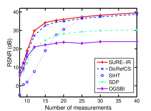
(a) RSNRs vs. $M$.

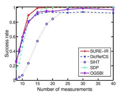
(b) Success rates vs. $M$

Figure 1: RSNRs and success rates of respective algorithms vs. $M$, $T=64$, $K=3$, and $\text{PSNR}=25\text{dB}$.

In the following, we examine the behavior of the respective algorithms under different scenarios. In Fig. 1, we plot the average RSNRs and success rates of respective algorithms as a function of the number of measurements $m$, where we set $T=64$, $K=3$, $\text{PSNR}=25\text{dB}$. Results are averaged over $10^{3}$ independent runs, with $\{\alpha_{k}\}$, $\{\omega_{k}\}$ and the sampling indices (used to obtain $\boldsymbol{y}$ from $\boldsymbol{y}_{T}$) randomly generated for each run. We see that the proposed method is superior to all other four methods in terms of both the RSNR and success rate. In particular, it is worth mentioning that the proposed method outperforms the SDP method which is guaranteed to find the global solution. This is probably because the log-sum penalty functional adopted by our algorithm is more sparse-encouraging than the atomic norm that is considered as the continuous analog to the $\ell_{1}$ norm for discrete signals. We also observe that the SIHT method yields poor performance for small $M$, mainly because the embedded subspace-based method (MUSIC or ESPRIT) for line spectral estimation barely works with a small number of data samples. The performance of the SIHT method, however, improves dramatically as $M$ increases. Moreover, we see that the OGSBI method, though using a very fine grid, still achieves performance inferior to the proposed SURE-IR and DicRefCS methods. In Fig. 2, we depict the RSNRs and success rates of respective algorithms vs. the number of complex sinusoids, $K$, where we set $T=64$, $M=30$, and $\text{PSNR}=25\text{dB}$. It can be observed that our proposed SURE-IR algorithm outperforms other methods by a big margin for a moderately large number of complex sinusoids $K$. For example, when $K=10$, a gain of over $10\text{dB}$ in RSNR can be achieved by our algorithm as compared with the DicRefCS and the SDP methods. This advantage makes our algorithm the most attractive for scenarios consisting of a moderate or large number of sinusoid components. The recovery performance of respective algorithms under different peak signal-to-noise ratios (PSNRs) is plotted in Fig. 3, where we choose $M=10$, $T=64$, and $K=3$. We see that our proposed SURE-IR method presents uniform superiority over other methods under different PSNRs.

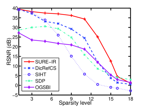
(a) RSNRs vs. $K$.

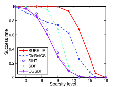
(b) Success rates vs. $K$

Figure 2: RSNRs and success rates of respective algorithms vs. $K$, $T=64$, $M=30$, and $\text{PSNR}=25\text{dB}$.

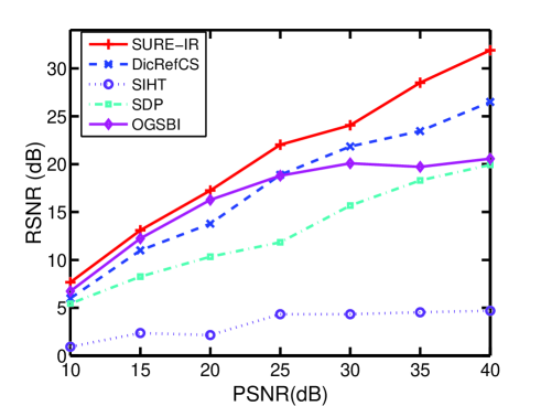
(a) RSNRs vs. PSNR.

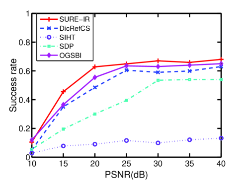
(b) Success rates vs. PSNR.

Figure 3: RSNRs and success rates of respective algorithms vs. PSNR, $T=64$, $M=10$, and $K=3$.

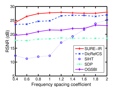
(a) RSNRs vs. $\mu$.

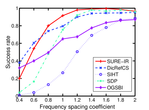
(b) Success rates vs. $\mu$.

Figure 4: RSNRS and success rates of respective algorithms vs. the frequency spacing coefficient $\mu$, $T=64$, $M=20$, and $\text{PSNR}=15\text{dB}$.

We now examine the ability of respective algorithms in resolving closely-spaced frequency components. The signal $\boldsymbol{y}$ is assumed a mixture of two complex sinusoids with the frequency spacing $d_{f}\triangleq\frac{1}{2\pi}(\omega_{1}-\omega_{2})=\mu/T$, where $\mu$ is the frequency spacing coefficient ranging from $0.4$ to $2$. Fig. 4 shows RSNRs and success rates of respective algorithms vs. the frequency spacing coefficient $\mu$, where we set $T=64$, $M=20$, and $\text{PSNR}=15\text{dB}$. Results are averaged over $10^{3}$ independent runs, with one of the two frequencies (the other frequency is determined by the frequency spacing) and the set of sampling indices randomly generated for each run. We observe that when the two frequency components are very close to each other, e.g. $\mu=0.6$, the SDP and the SIHT can hardly identify the true frequency parameters, whereas the SURE-IR and the DicRefCS are still capable of resolving these two closely-spaced components with decent success rates. Although the DicRefCS method slightly outperforms (in terms of the success rate) the SURE-IR method in the very small frequency spacing regime, it is quickly surpassed by the SURE-IR method as the frequency spacing increases.

Our last experiment tests the recovery performance of respective algorithms using a real-world amplitude modulated (AM) signal [24, 7] that encodes the message appearing in the top left corner of Fig. 6. The signal was transmitted from a communication device using carrier frequency $\omega_{c}=8.2$kHz, and the received signal was sampled by an analog-digital converter (ADC) at a rate of $32$kHz. The sampled signal has a total number of $32768$ samples. For the sake of computational efficiency, in our experiment, the AM signal is divided into a number of short-time segments, each consisting of $T=1024$ data samples. For each segment, we randomly select $M$ data samples, based on which we use respective algorithms to recover the whole segment. After all segments are reconstructed, we perform AM demodulation on the recovered signal to reconstruct the original message. The RSNR is then computed using the reconstructed message and the true message. Fig. 5 plots the RSNRs of respective algorithms vs. the ratio $M/T$ (the SDP method was not included in this experiment due to its prohibitive computational complexity when the signal dimension is large). We see that our proposed SURE-IR method offers the best performance and presents a significant performance advantage over the other algorithms for a small ratio $M/T$, where data acquisition is more beneficial due to high compression rates. In particular, when $M/T=0.02$, all the other three methods (DicRefCS, SIHT and OGSBI) fail to provide an accurate reconstruction, while our proposed algorithm still renders a decent recovery accuracy. Figs. 6 and 7 show the true message and the messages recovered by respective algorithms, where $M$ is set to $20$ and $100$, respectively. It can be seen that our proposed algorithm can obtain a fairly accurate reconstruction of the original signal even with as few as $M=20$ measurements, whereas the messages reconstructed by the SIHT and the OGSBI methods are highly smeared/distorted.

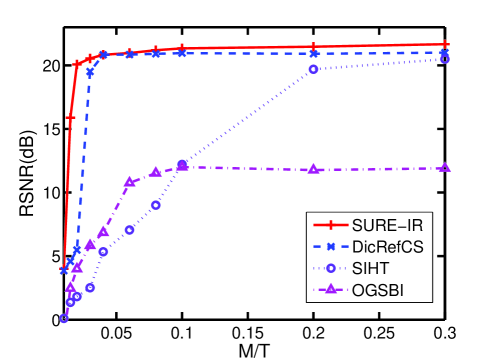
Figure 5: RSNRs of respective algorithms vs. the ratio $M/T$.

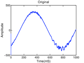
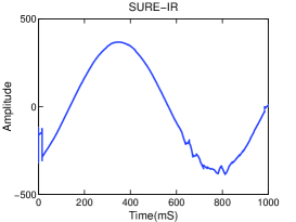
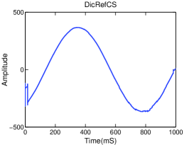
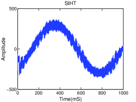
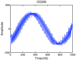
Figure 6: The true message and the messages reconstructed by respective algorithms, $M=100$.

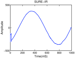
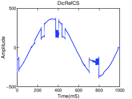
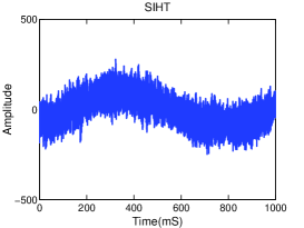
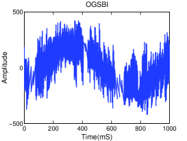
Figure 7: The true message and the messages reconstructed by respective algorithms, $M=20$.

VIII Conclusions

This paper studied the super-resolution compressed sensing problem where the sparsifying dictionary is characterized by a set of unknown parameters in a continuous domain. Such a problem arises in many practical applications such as direction-of-arrival estimation and line spectral estimation. By resorting to the majorization-minimization approach, we developed a generalized iterative reweighted $\ell_{2}$ algorithm for joint dictionary parameter learning and sparse signal recovery. The proposed algorithm iteratively decreases a surrogate function majorizing a given objective function, leading to a gradual and interweaved iterative process to refine the unknown parameters and the sparse signal. Simulation results show that our proposed algorithm effectively overcomes the grid mismatch problem and achieves a super-resolution accuracy in resolving the unknown frequency parameters. The proposed algorithm also demonstrates superiority over several existing super-resolution compressed sensing methods in resolving the unknown parameters and reconstructing the original signal.

Appendix A Derivative of $f(\boldsymbol{\theta})$ W.R.T. $\boldsymbol{\theta}$

Define

$$\boldsymbol{X}\triangleq\boldsymbol{A}(\boldsymbol{\theta})\big{(}\boldsymbol{A}^{H}(\boldsymbol{\theta})\boldsymbol{A}(\boldsymbol{\theta})+\lambda\boldsymbol{D}^{(t)}\big{)}^{-1}\boldsymbol{A}^{H}(\boldsymbol{\theta})$$

Using the chain rule, the first derivative of $f(\boldsymbol{\theta})$ with respect to $\theta_{i}$, $\forall i$ can be computed as

$$\frac{\partial f(\boldsymbol{\theta})}{\partial\theta_{i}}=\text{tr}\bigg{\{}\bigg{(}\frac{\partial f(\boldsymbol{\theta})}{\partial\boldsymbol{X}}\bigg{)}^{T}\frac{\partial\boldsymbol{X}}{\partial\theta_{i}}\bigg{\}}+\text{tr}\bigg{\{}\bigg{(}\frac{\partial f(\boldsymbol{\theta})}{\partial\boldsymbol{X}^{\ast}}\bigg{)}^{T}\frac{\partial\boldsymbol{X}^{\ast}}{\partial\theta_{i}}\bigg{\}}$$

where $\boldsymbol{X}^{\ast}$ donates the conjugate of the complex matrix $\boldsymbol{X}$, and

$$\frac{\partial f(\boldsymbol{\theta})}{\partial\boldsymbol{X}} =\frac{\partial}{\partial\boldsymbol{X}}\text{tr}\{-\boldsymbol{y}\boldsymbol{y}^{H}\boldsymbol{X}\}=-(\boldsymbol{y}\boldsymbol{y}^{H})^{T}$$

$$\frac{\partial f(\boldsymbol{\theta})}{\partial\boldsymbol{X}^{\ast}} =\frac{\partial}{\partial\boldsymbol{X}^{\ast}}\text{tr}\{-\boldsymbol{y}\boldsymbol{y}^{H}\boldsymbol{X}\}=\boldsymbol{0}$$

$$\frac{\partial\boldsymbol{X}}{\partial\theta_{i}} =\frac{\partial}{\partial\theta_{i}}\bigg{(}\boldsymbol{A}(\boldsymbol{\theta})\big{(}\boldsymbol{A}^{H}(\boldsymbol{\theta})\boldsymbol{A}(\boldsymbol{\theta})+\lambda^{-1}\boldsymbol{D}^{(t)}\big{)}^{-1}\boldsymbol{A}^{H}(\boldsymbol{\theta})\bigg{)}$$

$$=\frac{\partial\boldsymbol{A}(\boldsymbol{\theta})}{\partial\theta_{i}}\big{(}\boldsymbol{A}^{H}(\boldsymbol{\theta})\boldsymbol{A}(\boldsymbol{\theta})+\lambda^{-1}\boldsymbol{D}^{(t)}\big{)}^{-1}\boldsymbol{A}^{H}(\boldsymbol{\theta})$$

$$\quad+\boldsymbol{A}(\boldsymbol{\theta})\big{(}\boldsymbol{A}^{H}(\boldsymbol{\theta})\boldsymbol{A}(\boldsymbol{\theta})+\lambda^{-1}\boldsymbol{D}^{(t)}\big{)}^{-1}\frac{\partial\boldsymbol{A}^{H}(\boldsymbol{\theta})}{\partial\theta_{i}}$$

$$\quad+\boldsymbol{A}(\boldsymbol{\theta})\big{(}\boldsymbol{A}^{H}(\boldsymbol{\theta})\boldsymbol{A}(\boldsymbol{\theta})+\lambda^{-1}\boldsymbol{D}^{(t)}\big{)}^{-1}\bigg{(}\frac{\partial\boldsymbol{A}^{H}(\boldsymbol{\theta})}{\partial\theta_{i}}\boldsymbol{A}(\boldsymbol{\theta})$$

$$\quad+\boldsymbol{A}^{H}(\boldsymbol{\theta})\frac{\partial\boldsymbol{A}(\boldsymbol{\theta})}{\partial\theta_{i}}\bigg{)}\big{(}\boldsymbol{A}^{H}(\boldsymbol{\theta})\boldsymbol{A}(\boldsymbol{\theta})+\lambda^{-1}\boldsymbol{D}^{(t)}\big{)}^{-1}\boldsymbol{A}^{H}(\boldsymbol{\theta})$$

References

- [1] G. Tang, B. N. Bhaskar, B. Recht, and P. Shah, “Compressed sensing off the grid,” Available at http://arxiv.org/abs/1207.6053, 2012.
- [2] E. Candès and C. Fernandez-Granda, “Towards a mathematical theory of super-resolution,” Communications on Pure and Applied Mathematics, to appear.
- [3] Z. Yang, L. Xie, and C. Zhang, “Off-grid direction of arrival estimation using sparse Bayesian inference,” IEEE Trans. Signal Processing, vol. 61, no. 1, pp. 38–42, Jan. 2013.
- [4] Y. Chi, L. L. Scharf, A. Pezeshki, and A. R. Calderbank, “Sensitivity to basis mismatch in compressed sensing,” IEEE Trans. Signal Processing, vol. 59, no. 5, pp. 2182–2195, May 2011.
- [5] L. Hu, J. Zhou, Z. Shi, and Q. Fu, “A fast and accurate reconstruction algorithm for compressed sensing of complex sinusoids,” IEEE Trans. Signal Processing, vol. 61, no. 22, pp. 5744–5754, Nov. 2013.
- [6] A. Fannjiang and W. Liao, “Coherence pattern-guided compressive sensing with unresolved grids,” SIAM J. Imaging Sciences, vol. 5, no. 1, pp. 179–202, 2012.
- [7] M. F. Duarte and R. G. Baraniuk, “Spectral compressive sensing,” Applied and Computational Harmonic Analysis, vol. 35, pp. 111–129, 2013.
- [8] L. Hu, Z. Shi, J. Zhou, and Q. Fu, “Compressed sensing of complex sinusoids: An approach based on dictionary refinement,” IEEE Trans. Signal Processing, vol. 60, no. 7, pp. 3809–3822, 2012.
- [9] I. F. Gorodnitsky and B. D. Rao, “Sparse signal reconstructions from limited data using focuss: A re-weighted minimum norm algorithm,” IEEE Trans. Signal Processing, vol. 45, no. 3, pp. 699–616, Mar. 1997.
- [10] B. D. Rao and K. Kreutz-Delgado, “An affine scaling methodology for best basis selection,” IEEE Trans. Signal Processing, vol. 47, no. 1, pp. 187–200, Jan. 1999.
- [11] E. Candès, M. Wakin, and S. Boyd, “Enhancing sparsity by reweighted minimization,” Journal of Fourier Analysis and Applications, vol. 14, pp. 877–905, Dec. 2008.
- [12] R. Chartrand and W. Yin, “Iterative reweighted algorithm for compressive sensing,” in IEEE International Conference on Acoustics, Speech, and Signal Processing, Las Vegas, Nevada, USA, 2008.
- [13] D. Wipf and S. Nagarajan, “Iterative reweighted and methods for finding sparse solutions,” IEEE Journals of Selected Topics in Signal Processing, vol. 4, no. 2, pp. 317–329, Apr. 2010.
- [14] J. Fang, J. Li, Y. Shen, H. Li, and S. Li, “Super-resolution compressed sensing: an iterative reweighted algorithm for joint parameter learning and sparse signal recovery,” IEEE Signal Processing Letters, vol. 21, no. 6, pp. 761–765, June 2014.
- [15] B. A. Olshausen and D. J. Field, “Emergence of simple-cell receptive field properties by learning a sparse code for natural images,” Nature, vol. 381, pp. 607–609, June 1996.
- [16] Y. Shen, J. Fang, and H. Li, “Exact reconstruction analysis of log-sum minimization for compressed sensing,” IEEE Signal Processing Letters, vol. 20, pp. 1223–1226, Dec. 2013.
- [17] K. Lange, D. Hunter, and I. Yang, “Optimization transfer using surrogate objective functions,” Journal of Computational and Graphical Statistics, vol. 9, no. 1, pp. 1–20, Mar. 2000.
- [18] F. Bauer and M. A. Lukas, “Comparing parameter choice methods for regularization of ill-posed problems,” Mathematics and Computers in Simulation, vol. 81, no. 9, pp. 1795–1841, May 2011.
- [19] M. Tipping, “Sparse Bayesian learning and the relevance vector machine,” Journal of Machine Learning Research, vol. 1, pp. 211–244, 2001.
- [20] S. Ji, Y. Xue, and L. Carin, “Bayesian compressive sensing,” IEEE Trans. Signal Processing, vol. 56, no. 6, pp. 2346–2356, June 2008.
- [21] J. Fang, Y. Shen, H. Li, and P. Wang, “Pattern-coupled sparse Bayesian learning for recovery of block-sparse signals,” IEEE Trans. Signal Processing, vol. 63, no. 2, pp. 360–372, Jan. 2015.
- [22] S. F. Cotter, B. D. Rao, K. Engan, and K. Kreutz-Delgado, “Sparse solutions to linear inverse problems with multiple measurement vectors,” IEEE Trans. Signal Processing, vol. 53, no. 7, pp. 2477–2488, July 2005.
- [23] G. Tang, B. N. Bhaskar, and B. Recht, “Near minimax line spectral estimation,” Available at http://arxiv.org/abs/1303.4348v2, 2013.
- [24] J. A. Tropp, J. N. Laska, M. F. Duarte, J. K. Romberg, and R. G. Baraniuk, “Beyond Nyquist: efficient sampling of sparse bandlimited signals,” IEEE Trans. Information Theory, vol. 56, no. 1, pp. 520–544, Jan. 2010.