Estimation of the methylation pattern distribution from deep sequencing data

Abstract

Motivation: Bisulphite sequencing enables the detection of cytosine methylation. The sequence of the methylation states of cytosines on any given read forms a methylation pattern that carries substantially more information than merely studying the average methylation level at individual positions. In order to understand better the complexity of DNA methylation landscapes in biological samples, it is important to study the diversity of these methylation patterns. However, the accurate quantification of methylation patterns is subject to sequencing errors and spurious signals due to incomplete bisulphite conversion of cytosines.

Results: A statistical model is developed which accounts for the distribution of DNA methylation patterns at any given locus. The model incorporates the effects of sequencing errors and spurious reads, and enables estimation of the true underlying distribution of methylation patterns.

Conclusions: Calculation of the estimated distribution over methylation patterns is implemented in the R Bioconductor package MPFE. Source code and documentation of the package are also available for download at http://bioconductor.org/packages/3.0/bioc/html/MPFE.html.

¹Mathematical Sciences Institute, Australian National University, Canberra
² Research School of Biology, Australian National University, Canberra
³ School of Mathematics and Statistics, University of New South Wales, Sydney

Introduction

Epigenetic regulations are involved in a broad range of biological processes, including development, tissue homeostasis, learning and memory, as well as various diseases such as obesity and cancer [1, 2, 3].

DNA methylation is one of the best studied epigenetic molecular mechanisms. It consists of the addition of a methyl group to the cytosine residues (C) of a DNA molecule. In animals, DNA methylation usually takes place in the CpG context: cytosines followed by a guanine (G) residue.

DNA methylation modulates gene expression through a variety of mechanisms. In vertebrates, methylation in the promoter region usually has a repressive effect on transcription initiation. By contrast, methylation of gene bodies is generally associated with an active transcriptional state and has been shown to play an important role in the control of alternative splicing [4, 5].

The diverse and subtle effects of DNA methylation enable a given genome to produce different phenotypic outputs as part of a developmental program or in response to environmental factors. This has fundamental implications at the organismal level, where DNA methylation plays an important role in phenotypic plasticity [6]. This is also important at the cellular level to create diverse cell types, tissues and organs all based on the same genome. DNA methylation patterns can thus change from one cell type to another or within a cell under different conditions [7].

The diversity of methylation patterns in a sample can be studied with a single base pair resolution using the bisulphite sequencing technique [8]. When DNA is treated with bisulphite, the unmethylated cytosines are converted to uracils with a high (albeit not complete) efficiency, whereas the methylated cytosines remain as cytosines. A library is prepared from the bisulphite treated DNA by fragmenting to lengths of approximately 200 bp and PCR amplified. During this amplification process, uracils are replicated as thymines (T). The DNA library is then sequenced and the resulting reads are mapped to a reference. Within each read, CpG dinucleotides which have been converted to TpG are recognised as unmethylated, and unconverted CpG dinucleotides are recognised as methylated.

A common type of analysis carried out with this type of data is to estimate, for each cytosine, the global methylation level of a sample, namely, the average methylation level across all DNA strands in all the cells represented in that sample. This is usually done by correcting for the fact that bisulphite conversion is not a complete reaction (for instance, see [4, 9]).

However, this type of analysis only considers the methylation level at individual positions and is oblivious to the fact that cytosines present on a given read represent a broader snapshot of the methylation landscape on a particular strand of DNA. One can therefore gain a significantly deeper insight into the complexity of DNA methylation landscapes by reconstituting the methylation patterns that are physically present on the same sequence, and thus come from the same cell. Each read can be seen as containing a small number of binary labelled CpG sites: 1 for methylated, 0 for unmethylated and represents the methylation pattern of a given strand of DNA in one particular cell. This approach is of particular interest when studying complex biological samples that contain a mixture of cell types, for instance a tumour or a whole insect brain. It gives a much more detailed picture about the diversity of DNA methylation in a sample than simply looking at the methylation level at each position.

The approach of looking at methylation patterns instead of individual CpG sites can be hampered by the lack of sequencing coverage depth. For reasons of cost, most whole genome bisulphite sequencing studies have a mean genomic coverage in the 10-100 range. If the underlying sample contains hundreds of methylation patterns, they cannot be sampled representatively.

As an alternative, in order to reach a high coverage, researchers have often focussed on specific loci, either by sequencing PCR amplicons of bisulphite converted DNA, or by reduced representation bisulphite sequencing, or by using a capture assay (for review see [10]). In this paper, we focus on the analysis of amplicon data, but our method is widely applicable to other sequencing approaches.

The problem of determining methylation patterns in the original sample from the observed data is non trivial. The purpose of this paper is to infer formally the probability distribution over all possible methylation profiles defined by the population of epigenomes at a given locus.

Results

Synthetic data

The probability distribution over methylation patterns at a given locus from from bisulphite sequencing data is estimated via an algorithm described below in the Methods section. The algorithm is implemented as an R Bioconductor [11] package MPFE (for Methylation Patterns Frequency Estimation).

As the true distribution over methylation patterns is always unknown in the laboratory, we have constructed a number of synthetic data sets to test the effectiveness of the algorithm. For a locus with $n$ CpG sites we prescribe a true distribution $\theta_{k}$, $k=1,\ldots,2^{n}$, over the $2^{n}$ possible methylation patterns. We simulate from these patterns a set of $N_{\rm read}$ initial reads, each labelled with its ‘true’ methylation pattern, and then redistribute the reads among patterns according to the statistical model described in the Methods section to simulate errors due to incomplete bisulphite conversion and sequencing errors. Incomplete conversion is specified by a non-conversion rate parameter $\epsilon$ equal to the probability that an unmethylated cytosine will fail to convert. Its value is typically of order $10^{-2}$, and will be assumed in our simulations to be estimated independently from the rate of conversion of non-CpG cytosines. For instance, it could be calculated based on sequences known a priori not to be methylated. The sequencing error rates are specified by a vector $\eta=(\eta_{1},...,\eta_{n})$, where $\eta_{s}\sim O(10^{-2})$ is the probability that site $s$ is methylated but registers as unmethylated and vice versa. These two sources of error can generate spurious methylation patterns, that is, patterns for which the observed read count $y_{k}$ is non-zero when the true frequency of the pattern, $\theta_{k}$, is zero. The aim is to assess the ability of the algorithm to recover the true distribution $\theta_{k}$ from a set of observed read counts $y_{k}$, and, more specifically, determine whether spurious patterns can be identified.

The algorithm can be run in two possible modes: a slow mode, which performs a complete calculation over all possible $2^{n}$ methylation patterns, and a (default) fast mode which assumes $\theta_{k}=0$ for any pattern for which the observed read count $y_{k}$ is zero. Because of the exponential growth in the number of patterns, we find in general that use of the function in the slow mode becomes computationally prohibitive for $n>8$. However, there is very little difference in the computed results between the two modes (see below). Furthermore, the number of realised patterns tends to be relatively small and the performance of the function is adequate even for large $n$.

Figure 1 shows the results of analysing synthetic data in the slow mode at a locus with $n=6$ CpG sites, a non-conversion rate $\epsilon=0.005$, sequencing errors $\eta=(0.008,0.006,0.006,0.006,0.006,0.008)$ to model a signal that degrades towards the ends of the reads, and a total number of reads $N_{\rm read}=2000$.

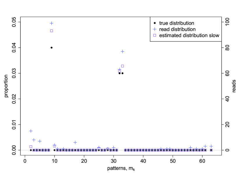
Figure 1: The ‘true’ distribution $\theta_{k}$ (black dots), observed read counts $y_{k}$ (blue pluses) and estimated distribution $\hat{\theta}_{k}$ (purple squares) over $2^{n}$ methylation patterns for synthetic data with $n=6$ CpG sites. The non-conversion rate is set to be $\epsilon=0.005$, the sequencing errors are set to be $\eta=(0.008,0.006,0.006,0.006,0.006,0.008)$, the total number of reads is $N_{\rm read}=2000$ and the estimated distribution was calculated using the slow version of the algorithm which estimates a distribution over all $64$ possible patterns. Methylation patterns are labelled lexicographically from $m_{1}=000000$ to $m_{64}=111111$. Data for patterns $m_{1}$, $m_{62}=111101$, and $m_{64}$ are beyond the range of the plot, but are listed in Table 1.

Table 1: Comparison between estimates $\hat{\theta}_{i}$ of the true methylation distribution $\theta_{i}$ calculated with the slow and fast implementations of our algorithm for the dataset of Figure 1. $y_{i}$ is the number of observed reads for pattern $i$ and $N_{\rm read}$ is the total number of reads.

Patterns	$\theta_{i}$	$y_{i}$	$y_{i}/N_{\rm read}$	$\hat{\theta}_{i}$ (slow)	$\hat{\theta}_{i}$ (fast)
000000	0.50	907	0.4535	0.4813	0.4812
000001	0.00	15	0.0075	0.0013	0.0013
000010	0.00	8	0.0040	0	0
000100	0.00	7	0.0035	0	0
001000	0.04	99	0.0495	0.0466	0.0466
001001	0.00	4	0.0020	0.0016	0.0014
001010	0.00	1	0.0005	0	0
001100	0.00	1	0.0005	0	0
010000	0.00	6	0.0030	0	0
011000	0.00	2	0.0010	0.0007	0.0004
011011	0.00	1	0.0005	0.0005	0.0002
011101	0.00	2	0.0010	0	0
011111	0.03	63	0.0315	0.0308	0.0306
100000	0.03	77	0.0385	0.0328	0.0329
101101	0.00	1	0.0005	0	0
101111	0.00	1	0.0005	0	0
110000	0.00	1	0.0005	0	0.0000
110111	0.00	2	0.0010	0	0
111001	0.00	1	0.0005	0	0
111011	0.00	1	0.0005	0	0
111100	0.00	3	0.0015	0	0
111101	0.20	393	0.1965	0.2001	0.2013
111110	0.00	3	0.0015	0	0
111111	0.20	401	0.2005	0.2044	0.2040

The results for the patterns with a non-zero number of observed reads are also listed in Table 1. We observe that for almost all patterns the estimated distribution $\hat{\theta}_{k}$ is closer to the true distribution $\theta_{k}$ than the naive read proportion $y_{k}/N_{\rm read}$, the only exception being a slight shift in the wrong direction for the pattern $m_{64}(111111)$. The algorithm correctly identifies $14$ out of the $18$ spurious patterns. Note that our implementation of the algorithm registers whether, for any given pattern $k$, the estimate $\hat{\theta}_{k}$ is identically zero, that is, it makes a call as to whether the pattern is present or absent. In this example, no real pattern is classified as spurious.

Table 1 and Figure 2 illustrate the comparison between the slow and (default) fast implementations of the algorithm applied to the data which were analysed using the slow version in Figure 1. In general, when the number of CpG sites $n$ in an amplicon is large, it is expected that only a small faction of the $2^{n}$ possible patterns will be present. Furthermore, it is rare for a true pattern with $\theta_{k}>0$ to have zero counts as a result of incomplete bisulphite conversion or sequencing errors. For instance, in the example of Figure 1 none of the patterns with a positive true frequency $\theta_{k}$ had zero reads. For the remaining patterns, i.e. those plotted in Figure 2, there is no substantial difference between the two implementations of the algorithm. The fast implementation identifies one less spurious pattern than the slow implementation; that is pattern $110000$, however, it estimates a very low proportion, with $\hat{\theta}_{i}\mbox{(fast)}<10^{-4}$. From now on, the discussion focusses on the fast implementation.

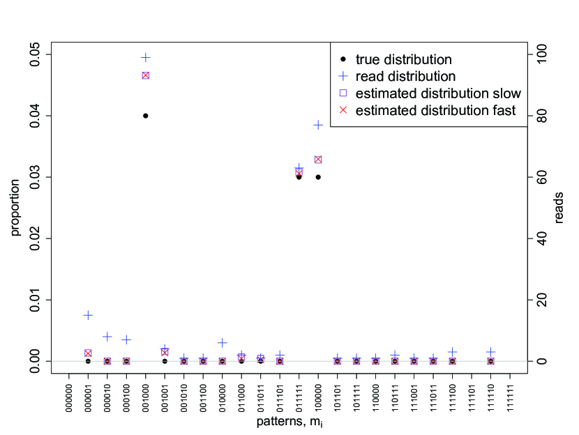
Figure 2: Comparison between estimates $\hat{\theta}_{i}$ calculated with the slow (purple squares) and fast (red crosses) implementations of our algorithm for the dataset of Figure 1. Only patterns with non-zero reads are shown. Data for the three patterns ($000000$, $111101$ and $111111$) which are beyond the range of the plot can be found in Table 1.

Figure 3 shows the results of applying the fast implementation of the algorithm to synthetic data modelled on biological data from a PCR amplicon in the honey bee Apis mellifera genome (see Biological data section). To obtain the dataset, the function was applied once to a biological dataset of $N_{\rm read}=730$ reads from an amplicon corresponding to a locus with $n=9$ CpG sites. To maintain a similar number of non-zero reads the ‘true’ distribution of the synthetic dataset was taken to be

$$\theta_{i}=\begin{cases}0&\text{if }\hat{\theta}_{i}^{\rm init}<0.05,\\ \hat{\theta}_{i}^{\rm init}&\text{otherwise},\end{cases}$$

where $\hat{\theta}_{i}^{\rm init}$ is the result of the initial application of the algorithm. Here the non-conversion parameter is $\epsilon=0.01$, and the sequencing error rate $\eta=0.02$ is taken to be uniform across all CpG sites.

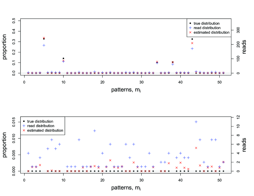
Figure 3: Comparison between the true distribution $\theta_{i}$, the simulated read distribution $y_{i}/N_{\rm read}$, and the estimated distribution $\hat{\theta}_{i}$ for a synthetic dataset based on amplicon data. Parameter values are $n=9$ CpG sites, total number of reads $N_{\rm read}=730$, non-conversion parameter $\epsilon=0.01$, and sequencing error rate $\eta=0.02$. The lower plot is an expanded version of the upper plot showing only patterns with low frequencies.

Of the $46$ spurious patterns in this dataset, $18$ are correctly identified and no false identifications of spurious patterns are made. For the $28$ failed identifications, the program generally estimates a lower estimate $\hat{\theta}_{i}$ than the read proportion $y_{i}/N_{\rm read}$.

Hypothesis testing

The effectiveness of our algorithm in identifying spurious patterns can be further gauged in terms of classical hypothesis testing. In the following definitions we only consider methylation patterns with non-zero reads $y_{i}$.

We set a threshold $K\in[0,1]$ and, using the estimated distribution $\hat{\theta}_{i}$ as a test statistic, declare pattern $i$ to be spurious when $\hat{\theta}_{i}\leq K$. Patterns are defined to be true or false positives or negatives according to the rules

$$\mbox{TP if }\hat{\theta}_{i}\leq K\mbox{ and }\theta_{i}=0,\qquad\mbox{FP if }\hat{\theta}_{i}\leq K\mbox{ and }\theta_{i}>0,$$

$$\mbox{TN if }\hat{\theta}_{i}>K\mbox{ and }\theta_{i}>0,\qquad\mbox{FN if }\hat{\theta}_{i}>K\mbox{ and }\theta_{i}=0.$$

True positive rates (TPR) and false positive rates (FPR) are defined in the usual way as

$$\mbox{TPR}=\frac{\mbox{TP}}{\mbox{TP}+\mbox{FN}},\qquad\mbox{FPR}=\frac{\mbox{FP}}{\mbox{FP}+\mbox{TN}}.$$

An analogous set of definitions applies using the raw data count proportions $y_{i}/N_{\rm read}$ as a test statistic.

Figure 4 shows the TPR curves for the data of Figure 2. It shows that using $\hat{\theta}_{i}$ results in a clear improvement in detecting which methylation patterns are likely to be a spurious artefact of incomplete conversion and reading error. The FPR curves for both test statistics are constantly zero for the same threshold range in the TPR graph.

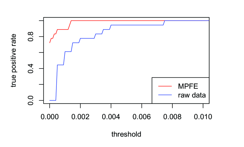
Figure 4: The TPR versus the threshold $K$ using the test statistic $\hat{\theta}_{i}$ (red curve) and $y_{i}/N_{\rm read}$ (blue curve) for the data of Figure 2.

Figure 5 shows the TPR curves for the synthetic data based on biological data from an amplicon analysed in Figure 3. Again we observe a clear improvement in detecting which methylation patterns are likely to be a spurious artefact of incomplete methylation and reading error.

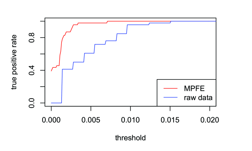
Figure 5: The TPR versus the threshold $K$ using the test statistic $\hat{\theta}_{i}$ (red curve) and $y_{i}/N_{\rm read}$ (blue curve) for the synthetic data analysed in Figure 3.

Biological data

Amplicons were obtained as described in [4]. Briefly, genomic DNA was extracted from brains of adult honeybee workers and treated with sodium bisulphite. A region of gene GB17113 (gene ID: 724724, a 6-phosphofructokinase) was then amplified by PCR and sequenced using the 454 technology.

Below we apply the fast algorithm to two examples from this dataset assuming a non-conversion rate of $\epsilon=0.01$ and a global sequencing error rate of $\eta=0.02$. The first example is shown in Figure 6 and Table 2. The parameter values are $n=8$ CpG sites, $36$ patterns with non-zero reads, and a total number of reads $N_{\rm read}=1793$.

Table 2: Estimated methylation distribution $\hat{\theta}_{i}$ for the data of Figure 6. The 36 patterns with non-zero reads are labelled $m_{i}$, $i=1,\ldots,36$ and $y_{i}$ are the observed read counts.

$i$	$m_{i}$	$y_{i}$	$y_{i}/N_{\rm read}$	$\hat{\theta}_{i}$
1	00000000	1265	0.7055	0.8706
2	00000001	52	0.0290	0.0059
3	00000010	32	0.0178	0
4	00000100	40	0.0223	0
5	00000110	3	0.0017	0.0010
6	00001000	75	0.0418	0.0189
7	00001001	1	0.0006	0
8	00001010	2	0.0011	0
9	00010000	36	0.0201	0
10	00010100	10	0.0056	0.0053
11	00100000	31	0.0173	0
12	00100001	2	0.0011	0.0003
13	00101000	1	0.0006	0
14	00110000	1	0.0006	0
15	01000000	20	0.0112	0
16	01000001	1	0.0006	0
17	01100000	39	0.0218	0.0240
18	01100001	4	0.0022	0.0016
19	01101000	1	0.0006	0
20	01110000	1	0.0006	0
21	01110100	1	0.0006	0
22	10000000	84	0.0468	0.0282
23	10000001	2	0.0011	0
24	10000010	5	0.0028	0.0013
25	10000100	14	0.0078	0.0070
26	10001000	1	0.0006	0
27	10010000	2	0.0011	0
28	10010100	8	0.0045	0.0044
29	10100000	2	0.0011	0
30	11000100	1	0.0006	0.0003
31	11010000	1	0.0006	0.0005
32	11100000	1	0.0006	0
33	11100100	2	0.0011	0.0006
34	11110000	2	0.0011	0.0007
35	11110100	42	0.0234	0.0255
36	11110110	8	0.0045	0.0039

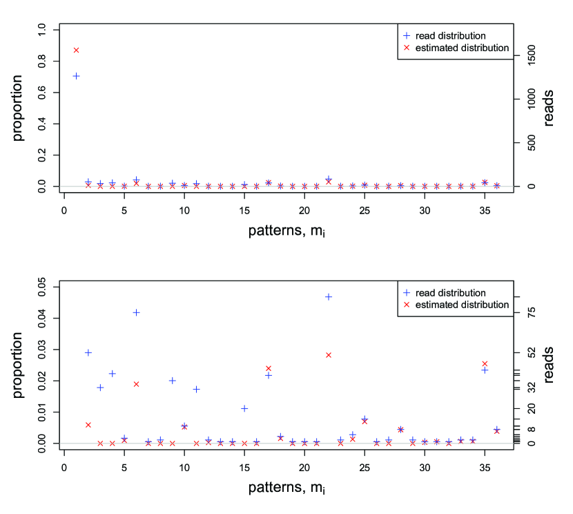
Figure 6: Estimated distribution $\hat{\theta}_{i}$ of the methylation patterns obtained for a honey bee amplicon. Parameter values are $n=8$ CpG sites, total number of reads $N_{\rm read}=1793$, non-conversion rate $\epsilon=0.01$, and sequencing error rate $\eta=0.02$. The lower plot is an expanded version of the upper plot showing only patterns with low frequencies. The 36 patterns with non-zero reads are listed in Table 2.

There are several observations:

1. $18$ patterns ($50\%$) are identified as spurious;

2. there are $11$ patterns with only $1$ read - our algorithm calls $9$ of them as spurious, while predicts the other $2$ patterns ($m_{30}$ and $m_{31}$) to exist;

3. patterns $m_{3}$, $m_{4}$, $m_{9}$ and $m_{11}$ with $>30$ reads each has a read proportion $y_{i}/N_{\rm read}\approx 2\%$, but are called as spurious.

Observations (i) and (ii) can be explained by the fact that the edit distance between the two patterns covered by a single read and any pattern observed to be highly abundant renders it unlikely that these patterns have arisen through sequencing errors or incomplete conversion. Observation (iii) arises because the spurious patterns with $>30$ reads are just one sequencing error or one incomplete conversion away from the most abundant pattern, $m_{0}$(00000000).

Figure 7 shows the second example, with $n=14$ CpG sites and $160$ patterns with non-zero reads. The total number of reads is $N_{\rm read}=2347$. In this case $47$ patterns are called as spurious.

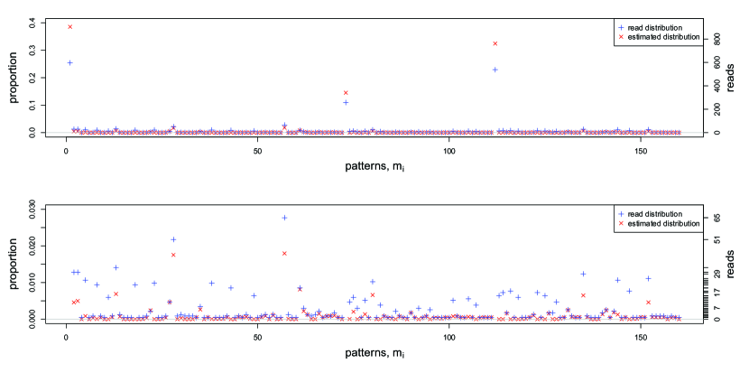
Figure 7: Estimated distribution $\hat{\theta}_{i}$ of the methylation patterns for a second amplicon from the honey bee genome. Parameter values are $n=14$ CpG sites, total number of reads $N_{\rm read}=2347$, non-conversion rate $\epsilon=0.01$, and sequencing error rate $\eta=0.02$. The lower plot is an expanded version of the upper plot showing only patterns with low frequencies.

Methods

Statistical model of bisulphite sequencing

We take as the starting point of our statistical model a population of epigenomes restricted to a locus containing $n$ CpG sites. Each member of the population within a given class is represented by a vector of non-independent binary valued random variables $\mathbf{K}=(K_{1},\ldots,K_{n})$, where each $K_{s}\in\{0,1\}$ labels the methylation state (1 for methylated, 0 for unmethylated) at the $s$-th CpG site at this locus. The population defines a methylation profile represented by the probability distribution of realising the pattern $\mathbf{k}=(k_{1},\ldots,k_{n})$ in a read randomly chosen from the population:

$$\theta_{\mathbf{k}}=\mbox{$\rm{Prob}$\,}(\mathbf{K}=\mathbf{k}),\quad\mathbf{k}\in\{0,1\}^{n}.$$ (1)

For convenience, from here on we will label the possible methylation patterns by the integers $k=1,\ldots,2^{n}$, and set $\theta_{\mathbf{k}}=\theta_{k}$, where $k-1$ is the integer whose binary representation is the methylation pattern $\mathbf{k}$.

Our aim is to estimate the distribution $\theta_{k}$ representing the relative abundance of methylation pattern $k$ from high throughput sequencing data consisting of a set of integer valued read counts $Y_{k}$. In a typical experiment, the number $n$ of CpG sites in an amplicon may be up $O(10^{2})$, and the total number of read counts $N_{\rm read}=\sum_{k=1}^{2^{n}}Y_{k}$ may be up to $O(10^{6})$.

The model takes into account two sources of error. First, the bisulphite conversion of unmethylated cytosine to uracil is not 100% efficient. There is a probability $\epsilon$ that an unmethylated CpG site will register as being methylated, where $\epsilon\sim O(10^{-2})$ can be estimated from the cytosines known not to be methylated (mitochondrial genome, chloroplastic genome, spike-ins, etc). The second type of error is caused by sequencing. For many applications this may be assumed for practical purposes to be site independent. However, to allow for effects such as degradation of the read quality towards the ends of the reads, we will assume there is a site-dependent probability $\eta_{s}\sim O(10^{-2})$ that if site $s$ is unmethylated it will register as methylated and vice versa. It follows that if the true methylation pattern of any given read is $\mathbf{K}$, but the read registers as being pattern $\mathbf{L}$, then

$$\mbox{$\rm{Prob}$\,}(L=\ell|K=k)=M_{k\ell},\quad k,\ell=1,\ldots 2^{n},$$ (2)

where

$$M=\bigotimes_{s=1}^{n}E_{s},$$ (3)

and

$$E_{s} = \left(\begin{array}[]{cc}1-\epsilon&\epsilon\\ 0&1\end{array}\right)\left(\begin{array}[]{cc}1-\eta_{s}&\eta_{s}\\ \eta_{s}&1-\eta_{s}\end{array}\right)$$ (8)

$$= \left(\begin{array}[]{cc}1-\epsilon-\eta_{s}+2\epsilon\eta_{s}&\epsilon+\eta_{s}-2\epsilon\eta_{s}\\ \eta_{s}&1-\eta_{s}\end{array}\right).$$ (11)

Eqs. (1) and (2) imply that probability that a random read will be the pattern $\ell$ is

$$\mbox{$\rm{Prob}$\,}(L=\ell)=\sum_{k=1}^{2^{n}}\theta_{k}M_{k\ell}=\phi_{\ell},$$ (12)

say. Assuming each read to be independent, for an experiment with a given total number of reads $N_{\rm read}$ the observed set of read counts represented by the random variable $Y_{\ell}$ has a multinomial distribution:

$$\mbox{$\rm{Prob}$\,}(Y_{\ell}=y_{\ell}|\phi)=\frac{N_{\rm read}!}{y_{1}!y_{2}!\ldots y_{2^{n}}!}{\phi_{1}}^{y_{1}}\ldots{\phi_{2^{n}}}^{y_{2^{n}}}.$$ (13)

In a recent applications note, [9] develop a statistical model for the distribution of the number of reads which register as being methylated in a pooled set of bisulphite-sequencing reads from CpG sites in a given region of a genome. Their model is mathematically equivalent to the $n=1$ version of the above model, and as such can be simplified to a single binomial distribution (see Supplementary Material).

Parameter estimation

The parameters of the distribution over methylation profiles, $\theta_{k}$, are estimated by maximising the log likelihood:

$$L(\theta|y)=\sum_{k=1}^{2^{n}}y_{k}\log\left(\sum_{j=1}^{2^{n}}\theta_{j}M_{jk}\right),$$ (14)

subject to the constraint that $(\theta_{1},\ldots,\theta_{2^{n}})$ lies in the $(2^{n}-1)$-dimensional simplex

$$S=\left\{\theta:\sum_{k=1}^{2^{n}}\theta_{k}=1,\theta_{k}\geq 0\right\}.$$ (15)

One may be tempted to use the usual formula, $\hat{\phi}_{\ell}=y_{\ell}/N_{\rm read}$, for the maximum likelihood estimate of multinomial parameters, and simply invert the matrix $M$ to recover $\hat{\theta}_{k}$. However this will not work for any realistic data because the matrix $M$ shrinks the simplex to a smaller volume. In practice many of the $y_{\ell}$ are zero, which leads to a naive estimate $\hat{\phi}_{\ell}$ on the boundary of the unshrunken simplex in $\phi$-space, and this boundary is not included in the shrunken simplex (see Fig. 8 for the $n=2$ case, in which the simplex is tetrahedron).

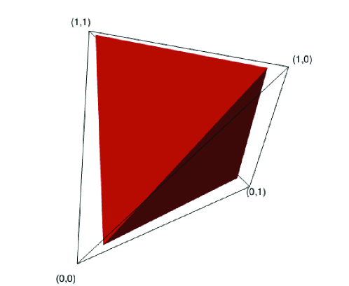
Figure 8: Boundary of the allowed simplex Eq. (15) for the parameters $\theta$, (black wire frame) and corresponding shrunken simplex containing allowed values of $\phi$ (red tetrahedron) for the case $n=2$ CpG sites, $\epsilon=0.05$, $\eta_{s}=0.02$. Numbers at the corners are the $2^{n}=4$ possible methylation patterns)

Instead we maximise the log likelihood over the allowed domain numerically by using the R function constrOptim(). Unfortunately the performance of this function becomes prohibitively slow for $n\gtrsim 8$ as the dimensionality of the parameter space grows exponentially. However, we have noticed in numerical simulations that if the observed counts $y_{k}$ are zero for a subset of the possible patterns, the corresponding estimates $\hat{\theta}_{k}$ are zero (or in rare cases, very close to zero) for the same subset. Thus we have implemented an algorithm which only searches over that part of the boundary of $S$ constrained by $\theta_{k}=0$ for those $k$ such that $y_{k}=0$. The algorithm remains reasonably efficient on a standard desktop computer provided the number of observed methylation patterns does not exceed about 200. This allows analysis of most realistic datasets while still addressing the biologically relevant question of identifying spurious methylation patterns which are the result of incomplete methylation.

Finally, to adjust for the fact that the function constrOptim() is of finite accuracy in locating the maximum of the log-likelihood, if the located maximum $\hat{\theta}$ is close to the boundary of the simplex, the value of the log-likelihood is also calculated at several nearby points on the boundary. If this results in a log-likelihood bigger than or equal to the maximum reported by constrOptim(), the appropriate point on the boundary is taken as the maximum likelihood estimate, and those patterns $m_{k}$ for which $\hat{\theta}_{k}\equiv 0$ are reported as being spurious reads.

Conclusions

We have developed an algorithm for estimating the true distribution of methylation patterns in at a genomic locus containing $n$ CpG sites. The algorithm, based on a constrained multinomial model, accounts for statistical variation due to incomplete bisulphite conversion and sequencing errors. The analysis differs from previous treatments in that the estimated distribution is a joint probability distribution over patterns which preserves maximal information pertaining to interaction between different CpG sites, as opposed to a pointwise measure of methylation at each site. A pointwise methylation estimate can, of course, be recovered from our estimated distribution as a marginal distribution. The algorithm is implemented as the R Bioconductor package MPFE.

Numerical experiments with realistic synthetic data indicate that the algorithm is able to identify the majority of the spurious observed methylation patterns, that is, patterns which are not present in the original library but are observed in the reads because of incomplete bisulphite conversion or sequencing errors. In general, our estimates are closer to the true distribution than the naive estimates given by the relative proportion of observed read counts for almost all patterns in each simulation (see Figures 2, 3, and Table 1).

Application of the algorithm to biological data consisting of bisulphite treated amplicon reads for a honeybee genomic sequence predicts that a correspondingly high proportion of observed methylation patterns in real data may indeed be spurious. However, our results also reveal an important number of real methylation patterns in this biological sample. This complexity of the methylation landscape is virtually undetectable when one only considers position-wise methylation level, but becomes apparent through our method.

Competing interests

The authors declare that they have no competing interests.

Author’s contributions

SF, CJB conceived and designed the project. SF prepared the datasets. PL, CJB developed the mathematical and statistical model, carried out the analysis and developed the software. PL, SF, CJB wrote the manuscript. All authors read and approved the final manuscript.

Additional Files

Additional file 1 — Comparison with Akman et al. (2014)

Analysis of the relationship of the statistical model used by Akman et al. [9] to our statistical model.

References

- [1] Cantone, I., Fisher, A.G.: Epigenetic programming and reprogramming during development. Nature structural & molecular biology 20(3), 282–289 (2013)
- [2] Day, J.J., Sweatt, J.D.: Dna methylation and memory formation. Nature neuroscience 13(11), 1319–1323 (2010)
- [3] Feinberg, A.P.: Phenotypic plasticity and the epigenetics of human disease. Nature 447(7143), 433–440 (2007)
- [4] Lyko, F., Foret, S., Kucharski, R., Wolf, S., Falckenhayn, C., Maleszka, R.: The honey bee epigenomes: differential methylation of brain DNA in queens and workers. PLoS Biol 8(11), 1000506 (2010)
- [5] Shukla, S., Kavak, E., Gregory, M., Imashimizu, M., Shutinoski, B., Kashlev, M., Oberdoerffer, P., Sandberg, R., Oberdoerffer, S.: Ctcf-promoted rna polymerase ii pausing links dna methylation to splicing. Nature 479(7371), 74–79 (2011)
- [6] Kucharski, R., Maleszka, J., Foret, S., Maleszka, R.: Nutritional control of reproductive status in honeybees via dna methylation. Science 319(5871), 1827–1830 (2008)
- [7] Hawkins, R.D., Hon, G.C., Lee, L.K., Ngo, Q., Lister, R., Pelizzola, M., Edsall, L.E., Kuan, S., Luu, Y., Klugman, S., et al.: Distinct epigenomic landscapes of pluripotent and lineage-committed human cells. Cell stem cell 6(5), 479–491 (2010)
- [8] Clark, S.J., Harrison, J., Paul, C.L., Frommer, M.: High sensitivity mapping of methylated cytosines. Nucleic Acids Res 22(15), 2990–2997 (1994)
- [9] Akman, K., Haaf, T., Gravina, S., Vijg, J., Tresch, A.: Genome-wide quantitative analysis of DNA methylation from bisulphite sequencing data. Bioinformatics 30(13), 1933–1934 (2014)
- [10] Lee, E.-J., Luo, J., Wilson, J.M., Shi, H.: Analyzing the cancer methylome through targeted bisulfite sequencing. Cancer Lett 340(2), 171–8 (2013). doi:10.1016/j.canlet.2012.10.040
- [11] Gentleman, R.C., Carey, V.J., Bates, D.M., et al.: Bioconductor: Open software development for computational biology and bioinformatics. Genome Biology 5, 80 (2004)