Stoner ferromagnetism of a strongly interacting Fermi gas in the quasirepulsive regime

Abstract

Recent advances in rapidly quenched ultracold atomic Fermi gases near a Feshbach resonance have brought about a number of interesting problems, in the context of observing the long-sought Stoner ferromagnetic phase transition. The possibility of experimentally obtaining a “quasirepulsive” regime in the upper branch of the energy spectrum due to the rapid quench is currently being debated, and the Stoner transition has mainly been investigated theoretically by using perturbation theory or at high polarization, due to the limited theoretical approaches in the strongly repulsive regime. In this work, we present a nonperturbative theoretical approach to the quasirepulsive upper branch of a Fermi gas near a broad Feshbach resonance, and we determine the finite-temperature phase diagram for the Stoner instability. Our results agree well with the known quantum Monte-Carlo simulations at zero temperature, and we recover the known virial expansion prediction at high temperature for arbitrary interaction strengths. At resonance, we find that the Stoner transition temperature becomes of the order of the Fermi temperature, around which the molecule formation rate becomes vanishingly small. This suggests a feasible way to observe Stoner ferromagnetism in the nondegenerate temperature regime.

I Introduction

An ultracold atomic Fermi gas with tunable contact interactions provides a paradigm to simulate strongly correlated many-body systems due to its unprecedented controllability Bloch2008 . With its strong attractions, it has paved the way for the crossover from Bardeen-Cooper-Schrieffer (BCS) superfluidity to Bose-Einstein condensation (BEC) of tightly bound fermionic pairs Giorgini2008 , while with its strong repulsions, it may lead to the confirmation of a text-book result of a ferromagnetic phase transition predicted nearly a century ago, the so-called Stoner ferromagnetism Stoner1933 . However, understanding the nature of this ferromagnetic transition is still an intriguing and controversial topic Massignan2014 . This is largely due to the fact that the experimental tunability of the repulsive interaction comes at the expense of severe atom loss Pekker2011 . The regime of strong effective repulsion can only be reached by rapidly quenching an attractively interacting atomic Fermi gas to the meta-stable upper branch of its energy spectrum near a Feshbach resonance Pricoupenko2004 . Initial experimental support of the Stoner ferromagnetic transition was reported in a strongly interacting Fermi gas of ⁶Li atoms Jo2009 . However, its existence in the same system was ruled out by more advanced spin-density fluctuation measurements Sanner2012 . Recent progress on repulsive polarons suggests that the Stoner transition may be observable by using a narrow Feshbach resonance Kohstall2012 or at low dimensions Koschorreck2012 . Triggered by these intriguing experimental observations, over the past few years, there has been considerable theoretical interests in Stoner ferromagnetism Duine2005 ; LeBlanc2009 ; Zhai2009 ; Conduit2009 ; Conduit2009-2 ; Dong2010 ; Liu2010a ; Liu2010b ; Zhang2010 ; Li2014 ; Pilati2010 ; Chang2011 ; Heiselberg2011 ; Saavedra2012 ; He2012 ; He2014a ; He2014b ; Cui2013 ; Massignan2013 .

Stoner’s original idea of a ferromagnetic transition is based on a simple first-order perturbation theory Stoner1933 , which at zero temperature predicts a smooth transition at $k_{F}a_{s}=\pi/2$ for a spin-population balanced system, where $k_{F}$ is the Fermi wave vector and $a_{s}$ is the s-wave scattering length. The application of the second-order perturbation theory improves the threshold to $k_{F}a_{s}\simeq 1.054$ Duine2005 , but the value is still too large to validate the perturbation theory. Recent zero-temperature quantum Monte Carlo simulations (QMC) Conduit2009-2 ; Pilati2010 ; Chang2011 , a lowest-order constraint variational calculation Heiselberg2011 , as well as a non-perturbative ladder approximation calculation He2012 , suggest instead a transition at $k_{F}a_{s}\simeq 0.8-0.9$. On the other hand, in the limit of large spin imbalance, where the system may behave like a weakly interacting gas of repulsive polarons, the ferromagnetic transition could be accurately determined Massignan2013 . Yet, a unified theoretical framework, which is valid at all temperatures and interaction strengths, has yet to be developed.

The purpose of this work is to present a nonperturbative theory of Stoner ferromagnetism at finite temperature, by performing controlled calculations both in a large-N expansion Nikolic2007 ; Veillette2007 ; Enss2012 and in a dimensional $\epsilon$ expansion Nishida2006 ; Nishida2007a ; Nishida2007b . Previously, the nonperturbative approach with a large-N expansion was applied to study the strongly interacting Bose gas LargeN-Bose , which is viewed as the upper branch of a Bose gas across a Feshbach resonance. Our prediction of Tan’s contact density agrees with the latest results from first-principles quantum Monte Carlo calculations Rossi2014 ; QMC-Bose , as shown in Fig. 1. In particular, the nonmonotonic temperature dependence of the two-body contact, predicted by our theory, is unambiguously confirmed. Therefore, we expect that the application of this nonperturbative theory to fermions will lead to a reliable description of the Stoner ferromagnetism at finite temperatures. A rigorous verification of our predictions can be obtained by confronting them with more advanced Monte Carlo simulations and experimental investigations of ferromagnetism at finite temperatures.

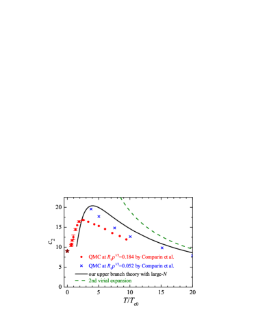
Figure 1: (Color online). The temperature dependence of the two-body contact $c_{2}$ of a unitary Bose gas. $c_{2}$ is in units of $\rho^{4/3}$, where $\rho$ is the density of the unitary Bose gas. $T_{c0}$ is the transition temperature of an ideal Bose gas with density $\rho$. The black solid line shows the prediction of our upper branch theory within the large-$N$ expansion approximation LargeN-Bose . It agrees reasonably well with the latest Monte Carlo simulation at both zero temperature (stars, from Ref. Rossi2014 ) and finite temperatures (solid circles and crosses at two different three-body parameters, from Ref. QMC-Bose ). The green dashed line is the second-order virial expansion result that is valid at high temperatures LargeN-Bose .

In this work, we find that the Stoner transition occurs at finite temperature in a strongly interacting but near-degenerate Fermi gas. The relatively high transition temperature makes the molecule formation rate vanishingly small, and thus the observation of the Stoner transition will no longer suffer from severe atom loss. Our prediction thereby paves the way towards experimental confirmation of the long-sought Stoner ferromagnetic phase transition. Our results may also be used to better understand the occurrence of ferromagnetism in many strongly correlated solid-state systems, including superconductors, metals, and insulators.

One crucial component of our finite-temperature theory is an appropriate definition of a many-body phase shift for the quasirepulsive upper branch. In an earlier study, it was realized that a description of quasirepulsive interaction may be achieved by excluding the in-medium bound-state contribution from the density equation within a Nozieres-Schmitt-Rink (NSR) approach Shenoy2011 . However, this treatment predicts an equilibrium switch between the upper and the lower branches near the resonance at high temperature and results in a wide forbidden area in the low-temperature phase diagram. Alternative spectral representation of the approach that takes into account an additional frequency-independent two-body term still suffers from a sudden drop in the spin susceptibility near the Feshbach resonance Palestini2012 . Here, we show that the clarification of the quasirepulsive upper branch, together with the controllable large-$N$ expansion and $\epsilon$ expansion, provides a reliable phase diagram at arbitrary temperatures and coupling strengths.

Our paper is organized as follows. In the next section (Sec. II), we review the theoretical framework of the large-$N$ expansion and the dimensional $\epsilon$ expansion, and we examine the usefulness of these two approaches for a strongly interacting Fermi gas in the attractive branch. We explain the definition of the upper branch, Eq. (12), and we provide a detailed proof of this definition from the viewpoint of the virial expansion. The technical proof may be skipped for the first reading. In Sec. III, we present the main results of our work, i.e., the Stoner transition at both zero temperature and finite temperature. A finite-temperature phase diagram is shown and the stability of the upper branch is briefly discussed. Finally, Sec. IV is devoted to conclusions and outlooks.

II Theory

We first adopt the large-N approach following the pioneering works by Nikolić et al. Nikolic2007 and Veillette et al. Veillette2007 for an attractive Fermi gas at the BEC-BCS crossover. An artificial small parameter, $1/N$, is introduced to organize the different diagrammatic contributions or scattering processes around the mean-field solution. The original theory is recovered in the limit of $N=1$. The motivation of the large-$N$ expansion is that there are no phase transitions with deceasing $N$, and the large-$N$ (i.e., mean-field) solution has the same symmetry as the original ground state at $N=1$. Therefore, we anticipate that the large-$N$ results connect smoothly to the physical results at $N=1$. One can then perform controlled calculations by including all diagrams up to a certain order in $1/N$. Although in our calculations we stop at the next-to-leading-order ($1/N$), systematic improvements could be achieved by going to higher orders. A complementary approach, which is similar in spirit, is the dimensional $\epsilon$ expansion. We will briefly discuss the $\epsilon$ expansion Nishida2006 ; Nishida2007a ; Nishida2007b at the end of this section.

II.1 Large-N expansion

We consider a three-dimensional spin-1/2 interacting Fermi gas with $N$ fermionic flavors ($i,j=1,\ldots,N$) for each spin degree of freedom $\sigma=\uparrow,\downarrow$, described by an action (setting the volume $V=1$ and $\hbar=k_{B}=1$) Nikolic2007 ; Veillette2007 ; Enss2012

$$\mathcal{S} = \int d^{3}\mathbf{x}d\tau\left[\sum_{i=1}^{N}\sum_{\sigma=\uparrow,\downarrow}\psi_{i\sigma}^{*}\left(\partial_{\tau}-\frac{\mathbf{\nabla}^{2}}{2m}-\mu\right)\psi_{i\sigma}\right.$$ (1)

$$\left.+\frac{U_{0}}{N}\sum_{i,j=1}^{N}\psi_{i\uparrow}^{*}\psi_{i\downarrow}^{*}\psi_{j\downarrow}\psi_{j\uparrow}\right],$$

where $\psi_{i\sigma}\left(\mathbf{x},\tau\right)$ are Grassmann fields representing fermionic species of equal mass $m$ and the imaginary time $\tau$ takes values from $0$ to the inverse temperature $\beta=1/T$. $\mu$ is the chemical potential and $U_{0}$ is the bare interaction strength to be renormalized in terms of the s-wave scattering length $a_{s}$ via the relation

$$\frac{m}{4\pi a_{s}}=\frac{1}{U_{0}}+\sum_{\mathbf{k}}\frac{1}{2\varepsilon_{{\bf k}}}$$ (2)

with $\varepsilon_{{\bf k}}=\mathbf{k}^{2}/(2m)$. The action possesses invariance under the symplectic group Sp(2N) and in the case of $N=1$ describes the usual spin-1/2 Fermi gas.

By decoupling the interaction term in the action via a standard Hubbard-Stratonovich transformation and integrating out the fermionic Grassmann fields, at the level of Gaussian fluctuations (i.e., the first nontrivial correction at the order of $1/N$), we obtain the pressure NSR1985 ; NSR1993 ; NSR2006 ; Liu2006

$$\frac{\mathcal{P}}{T}=2N\sum_{\mathbf{k}}\ln\left(1+e^{-\beta\xi_{\mathbf{k}}}\right)-\sum_{\mathbf{q},i\nu_{l}}\ln\left[-\Gamma^{-1}\left(\mathbf{q},i\nu_{l}\right)\right],$$ (3)

where $\xi_{\mathbf{k}}=\varepsilon_{{\bf k}}-\mu$ and $\Gamma(\mathbf{q},i\nu_{l})$ is the two-particle vertex function with bosonic Matsubara frequencies $\nu_{l}=2\pi lT$ ($l=0,\pm 1,\pm 2,\cdots$),

$$\Gamma^{-1}\left(\mathbf{q},i\nu_{l}\right)=\frac{m}{4\pi a_{s}}-\sum_{\mathbf{k}}\left[\frac{\gamma\left(\mathbf{q},\mathbf{k}\right)}{i\nu_{l}-\xi_{\mathbf{q}/2+\mathbf{k}}-\xi_{\mathbf{q}/2-\mathbf{k}}}+\frac{1}{2\varepsilon_{\mathbf{k}}}\right].$$ (4)

$\gamma(\mathbf{q},\mathbf{k})\equiv 1-f(\xi_{\mathbf{q}/2+\mathbf{k}})-f(\xi_{\mathbf{q}/2-\mathbf{k}})$ with the Fermi distribution $f(x)=1/(e^{\beta x}+1)$ includes (in-medium) Pauli blocking of pair fluctuations. By recalling that the vertex function is essentially the Green function of pairs, the pressure in Eq. (3) simply describes a non-interacting mixture of $2N$ fermionic species and the bosonic pairs Liu2006 . By converting the summation over Matsubara frequencies into an integral over real frequency and introducing an in-medium two-particle phase shift NSR1985 ; NSR1993 ; NSR2006

$$\delta(\mathbf{q},\omega)\equiv-{\rm Imln}[-\Gamma^{-1}(\mathbf{q},\omega+i0^{+})],$$ (5)

the contribution from the bosonic pairs can be rewritten as

$$\Delta\mathcal{P}=\sum_{\mathbf{q}}\int_{-\infty}^{+\infty}\frac{d\omega}{\pi}b(\omega)\delta\left(\mathbf{q},\omega\right),$$ (6)

where $b(\omega)=1/(e^{\beta\omega}-1)$ is the Bose distribution. According to standard scattering theory, the two-particle phase shift is associated with the density of state and increases by $\pi$ when a two-body bound state emerges NSR1985 . It should vanish precisely at $\omega=0$, as required by the integrability of Eq. (6).

For a unitary Fermi gas in the attractive (ground state) branch, the application of the large-$N$ expansion has been successful. At zero temperature, the predicted Bertsch parameter $\xi_{N}=0.279$ Veillette2007 is in reasonable agreement with the most recent experimental measurement $\xi=0.376\pm 0.005$ Ku2012 and quantum Monte Carlo result $\xi=0.37-0.38$ Forbes2011 ; Carlson2011 . The predicted inverse superfluid transition temperature, $(T_{F}/T_{c})_{N}=6.579$ Nikolic2007 , is also very close to the experimental data $(T_{F}/T_{c})_{N}=6.0\pm 0.5$ Ku2012 . Near the quantum critical point $\mu=0$, the large-N expansion approach was recently examined by Enss Enss2012 , by comparing the results for the equation of state and Tan’s contact with more favorable theoretical predictions (i.e., bold diagrammatic Monte Carlo, BDMC) or the accurate experimental data Ku2012 . It was shown that for the pressure $P$, there is excellent agreements (less than 4%) between the large-$N$ calculation $P_{N}=0.928nk_{B}T$ and the experimental data $P=0.891\pm 0.019nk_{B}T$ (or the BDMC data $P=0.90\pm 0.02nk_{B}T$) Enss2012 . There is also a similar good agreement for the entropy density $S/(Nk_{B})$. For Tan’s contact $C$, the large-$N$ prediction ($C_{N}=0.0789k_{F}^{4}$) is just 1.4% below the BDMC calculation ($C=0.080\pm 0.005k_{F}^{4}$). This is very impressive, given the simplicity of the large-$N$ calculation Enss2012 .

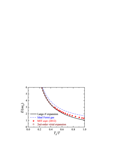
Figure 2: (Color online) Temperature dependence of the total energy of a unitary Fermi gas predicted by the large-$N$ expansion theory. The large-N expansion results (solid line) are compared with the accurate experimental measurement from the MIT group (solid circles) Ku2012 , as well as the second-order virial expansion prediction (empty squares) Liu2013 . The dot-dashed line is the energy of an ideal, non-interacting Fermi gas.

In Fig. 2, we provide our benchmark of the large-$N$ theory and systematically compare the large-$N$ predictions with the experimental results in the non-degenerate regime with $T>T_{F}$. The large-N expansion prediction for the universal energy agrees reasonably well with the recent experimental measurement by the MIT group Ku2012 and with the second-order virial expansion result at sufficiently large temperatures Liu2013 .

II.2 Phase shift of the upper branch

The above theory is only for the attractive branch (ground state). One crucial component of our finite-temperature theory for the quasirepulsive upper branch is an appropriate definition of a many-body phase shift.

For the attractive ground state, the phase shift $\delta_{\textrm{att}}\left(\mathbf{q},\omega\right)$ is generally positive, and the condition $\delta_{\textrm{att}}(\mathbf{q},\omega=0)=0$ is a sufficient criterion to determine the lowest temperature (i.e., $T_{c}$) for Cooper pairing instability. In the inset of Fig. 3, we show a typical phase shift for the attractive branch at $1/(k_{F}a_{s})=2$ with a chemical potential at Fermi energy, $\mu=\varepsilon_{F}=k_{F}^{2}/(2m)$. With increasing frequency, the phase shift jumps from 0 to $\pi$ at a critical value $\omega_{b}(\mathbf{q})$, where the vertex function develops a pole. This simply signals the existence of a two-body bound state. With further increasing frequency above the scattering threshold $\omega_{s}(\mathbf{q})=\mathbf{q}^{2}/(4m)-2\mu>\omega_{b}(\mathbf{q})$, the phase shift deviates from $\pi$ as the imaginary part of $-\Gamma^{-1}(\mathbf{q},\omega)$ is no longer zero, indicating the scattering continuum. We note that in this case the criterion $\delta_{\mathbf{\textrm{att}}}(\mathbf{q},\omega=0)=0$ is clearly not satisfied. This is because we have used an unrealistic large chemical potential for the attractive ground state. In a realistic solution, the chemical potential will be necessarily pinned by the Thouless criterion to a value slightly larger than half of the bound-state energy $-1/(ma_{s}^{2})$ NSR1985 .

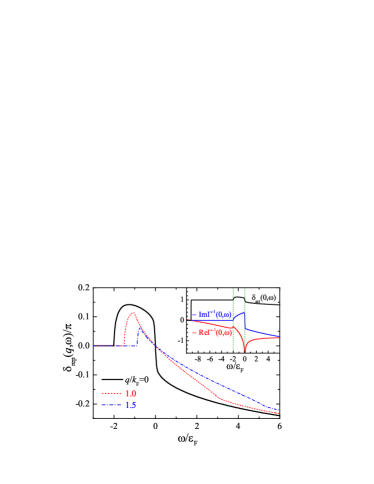
Figure 3: (Color online). The in-medium phase shift $\delta_{\textrm{rep}}(q,\omega)$ of a quasirepulsive Fermi gas at the interaction parameter $k_{F}a_{s}=0.5$ and $T=0$. We have taken a chemical potential $\mu=\varepsilon_{F}$, which is suitable for the weakly interacting regime. The inset shows the corresponding in-medium phase shift for an attractive Fermi gas $\delta_{\textrm{att}}(q=0,\omega)$, together with the real and imaginary parts of the negative inverse of the two-particle vertex function, $-\Gamma^{-1}(q=0,\omega)$.

For the quasirepulsive upper branch, we first notice that the two-body phase shift in vacuum is given by

$$\delta_{2{\rm B}}(E)=-{\rm Im}{\rm ln}\left[-\frac{1}{a_{s}}+\sqrt{-m(E+i0^{+})}\right].$$ (7)

For the BEC side with $a_{s}>0$, we have

$$\delta_{2{\rm B}}(E)=\left\{\begin{array}[]{r@{\quad,\quad}l}0&-\infty<E<\varepsilon_{{\rm B}}\\ \pi&\varepsilon_{{\rm B}}<E<0\\ \pi-\arctan(a_{s}\sqrt{mE})&E>0,\end{array}\right.$$ (11)

where $\varepsilon_{{\rm B}}=-1/(ma_{s}^{2})$ is the bound state energy level. The $\pi$-jump at $E=\varepsilon_{{\rm B}}$ shows clearly the existence of a bound state. Therefore, to define a quasirepulsive two-body system, the $\pi$-shift coming from the bound state should be subtracted. Inspired by this two-body picture, we find another repulsive solution for the phase shift, by considering a different branch cut for the argument of $-\Gamma^{-1}(\mathbf{q},\omega)$, which differs from $\delta_{\textrm{att}}$ by a constant shift $\pi$ from the scattering threshold:

$$\delta_{\textrm{rep}}\left(\mathbf{q},\omega\right)=\left[\delta_{\textrm{att}}\left(\mathbf{q},\omega\right)-\pi\right]\Theta\left[\omega-\omega_{s}\left(\mathbf{q}\right)\right].$$ (12)

In the following, we show that Eq. (12) is an appropriate prescription of the phase shift for the upper branch from the viewpoint of virial expansion Liu2013 . In brief, it is known that the bosonic contribution $\Delta\mathcal{P}$ contains all two-particle virial series to infinite order of the fugacity $z=e^{\beta\mu}$ Liu2013 . It can be expressed as

$$\Delta\mathcal{P}=\mathcal{P}^{(2)}=\sum_{n=2}^{\infty}\mathcal{P}_{n}^{(2)},$$ (13)

where $\mathcal{P}_{n}^{(2)}\propto z^{n}$ is the $n$-th two-particle virial contribution. Since the two-body energy spectrum is known exactly, we can precisely separate $\mathcal{P}_{n}^{(2)}$ into its contributions from the bound state and from the scattering continuum. By resumming only the scattering contributions to all orders in $z$, we obtain precisely the prescription (12).

At high temperature, the fugacity becomes small, $z=e^{\beta\mu}\ll 1$. The contribution of two-particle scattering process to the pressure can be expressed as Liu2013

$${\cal P}^{(2)}=\sum_{n=2}^{\infty}{\cal P}_{n}^{(2)}=\frac{2T}{\lambda_{{\rm dB}}^{3}}\sum_{n=2}^{\infty}b_{n}^{(2)}z^{n},$$ (14)

where $\lambda_{{\rm dB}}=[2\pi/(mT)]^{1/2}$ is the thermal de Broglie wavelength and $b_{n}^{(2)}$ is the two-particle contribution to the $n$-th virial coefficient.

The $n$-order contribution ${\cal P}_{n}^{(2)}$ can be obtained by making the virial expansion of the pressure $\Delta{\cal P}$. To this end, we put the dependence on the chemical potential $\mu$ into the distribution functions by using a new variable $E=\omega+2\mu-{\bf q}^{2}/(4m)$. Then we obtain

$${\cal P}^{(2)}=\sum_{{\bf q}}\int_{-\infty}^{\infty}\frac{dE}{\pi}b\left(E+\frac{{\bf q}^{2}}{4m}-2\mu\right)\delta(E,{\bf q}).$$ (15)

Here the phase shift $\delta(E,{\bf q})$ in terms of $E$ can be expressed as $\delta(E,{\bf q})=-{\rm Im}{\rm ln}\left[A(E,{\bf q})+iB(E,{\bf q})\right]$, where the functions $A(E,{\bf q})$ and $B(E,{\bf q})$ are given by

$$A(E,{\bf q}) = -\frac{1}{a_{s}}+\frac{4\pi}{m}{\rm p.v.}\sum_{{\bf k}}\left[\frac{\gamma({\bf k},{\bf q})}{E-2\varepsilon_{{\bf k}}}+\frac{1}{2\varepsilon_{{\bf k}}}\right],$$

$$B(E,{\bf q}) = -\frac{4\pi^{2}}{m}\sum_{{\bf k}}\gamma({\bf k},{\bf q})\delta(E-2\varepsilon_{{\bf k}}).$$ (16)

For $E>0$, p.v. stands for the principal value. The virial expansion of ${\cal P}^{(2)}$ can be worked out by making use of the expansions of the Bose and Fermi distribution functions. The distribution functions can be expanded as

$$b\left(E+\frac{{\bf q}^{2}}{4m}-2\mu\right)=\sum_{n=1}^{\infty}z^{2n}e^{-n\beta(E+\frac{{\bf q}^{2}}{4m})}$$ (17)

and

$$f\left(\varepsilon-\mu\right)=\sum_{n=1}^{\infty}z^{n}(-1)^{n-1}e^{-n\beta\varepsilon}.$$ (18)

Accordingly, the phase shift $\delta(E,{\bf q})$ can be expanded as

$$\delta(E,{\bf q})=\delta_{2{\rm B}}(E)+\sum_{n=1}^{\infty}z^{n}\phi_{n}(E,q),$$ (19)

where $\delta_{2{\rm B}}(E)$ is the two-body phase shift in the vacuum,

Now we consider the BEC side with $a_{s}>0$. According to the expansion (19) of the phase shift $\delta(E,{\bf q})$, we can divide the pressure ${\cal P}^{(2)}$ into four contributions.

(A) The first two contributions come from the leading-order expansion of the phase shift. Keeping only the vacuum two-body phase shift $\delta_{2{\rm B}}(E)$, we obtain

$${\cal P}_{2{\rm B}}^{(2)}=\sum_{n=1}^{\infty}z^{2n}\sum_{{\bf q}}e^{-\frac{n\beta{\bf q}^{2}}{4m}}\int_{-\infty}^{\infty}\frac{dE}{\pi}e^{-n\beta E}\delta_{2{\rm B}}(E).$$ (20)

The relative two-body motion and the center-of-mass motion are decoupled because $\delta_{2{\rm B}}(E)$ depends only on $E$. We can separate the two-body phase shift into its bound-state part $\delta_{{\rm b}}(E)$ and scattering-state part $\delta_{{\rm s}}(E)$. We have $\delta_{2{\rm B}}(E)=\delta_{{\rm b}}(E)+\delta_{{\rm s}}(E)$, where

$$\delta_{{\rm b}}(E) = \pi\Theta(E-\varepsilon_{{\rm B}}),$$

$$\delta_{{\rm s}}(E) = \left[\delta_{2{\rm B}}(E)-\pi\right]\Theta(E-\varepsilon_{{\rm B}}).$$ (21)

Accordingly, the pressure ${\cal P}_{2{\rm B}}^{(2)}$ can be divided into its bound-state contribution ${\cal P}_{{\rm b}}^{(2)}$ and its scattering-state contribution ${\cal P}_{{\rm s}}^{(2)}$. We have ${\cal P}_{2{\rm B}}^{(2)}={\cal P}_{{\rm b}}^{(2)}+{\cal P}_{{\rm s}}^{(2)}$, where

$${\cal P}_{{\rm b}}^{(2)} = \sum_{n=1}^{\infty}z^{2n}\sum_{{\bf q}}e^{-\frac{n\beta{\bf q}^{2}}{4m}}\int_{-\infty}^{\infty}\frac{dE}{\pi}e^{-n\beta E}\delta_{{\rm b}}(E),$$

$${\cal P}_{{\rm s}}^{(2)} = \sum_{n=1}^{\infty}z^{2n}\sum_{{\bf q}}e^{-\frac{n\beta{\bf q}^{2}}{4m}}\int_{-\infty}^{\infty}\frac{dE}{\pi}e^{-n\beta E}\delta_{{\rm s}}(E).$$ (22)

Notice that these two contributions are not simply separated by $E<0$ and $E>0$. Completing the integrals over ${\bf q}$ and $E$, we obtain

$${\cal P}_{{\rm b}}^{(2)} = \frac{2^{3/2}T}{\lambda_{{\rm dB}}^{3}}\sum_{n=1}^{\infty}\frac{z^{2n}}{n^{5/2}}e^{-n\beta\varepsilon_{{\rm B}}},$$

$${\cal P}_{{\rm s}}^{(2)} = \frac{2^{3/2}T}{\lambda_{{\rm dB}}^{3}}\sum_{n=1}^{\infty}\frac{z^{2n}}{n^{5/2}}\int_{0}^{\infty}\frac{dk}{\pi}e^{-\frac{n\beta k^{2}}{m}}\frac{d\delta(k)}{dk}.$$ (23)

Here $\delta(k)=-\arctan(ka_{s})$ is now the usual scattering phase shift without bound state. It becomes evident that ${\cal P}_{{\rm b}}^{(2)}$ and ${\cal P}_{{\rm s}}^{(2)}$ correspond to the bound-state and scattering-state contributions, respectively. For $n=1$, they recover the well-known Beth-Uhlenbeck formula of the second virial coefficient.

(B) The other two contributions come from the higher-order expansions of the phase shift which show explicitly the medium effect. These contributions can be called medium corrections and can be expressed as

$${\cal P}_{{\rm m}}^{(2)} = \sum_{n=1}^{\infty}\sum_{l=1}^{\infty}z^{2n+l}\sum_{{\bf q}}e^{-\frac{n\beta{\bf q}^{2}}{4m}}$$ (24)

$$\times\int_{-\infty}^{\infty}\frac{dE}{\pi}e^{-n\beta E}\phi_{l}(E,q).$$

We notice that the relative two-body motion and the center-of-mass motion cannot be separated for these contributions. To obtain the expansion coefficients $\phi_{n}(E,q)$, we need to evaluate the expansions for $A(E,{\bf q})$ and $B(E,{\bf q})$. We thus consider two regimes of $E$: $E<0$ and $E>0$. We will see that the bound-state and scattering-state contributions are separated by these two regimes.
(1) $E<0$. In this regime we have $B(E,{\bf q})=0$. The real part $A(E,{\bf q})$ can be expressed as

$$A(E,{\bf q})=-\frac{1}{a_{s}}+\sqrt{-mE}+\sum_{n=1}^{\infty}\frac{(-1)^{n-1}}{n}z^{n}{\cal A}_{n}(E,q),$$ (25)

where the expansion coefficients read

$${\cal A}_{n}(E,q)=\frac{16mT}{\pi q}e^{-\frac{n\beta q^{2}}{8m}}\int_{0}^{\infty}pdp\frac{e^{-\frac{n\beta p^{2}}{2m}}\sinh\frac{n\beta pq}{2m}}{p^{2}-mE}.$$ (26)

In this regime, the medium effect ($z\ll 1$) induces a shift of the bound state pole. Therefore, we have formally

$$\phi_{l}(E,q)=\pi\sum_{\nu=0}^{l-1}\delta^{(\nu)}(E-\varepsilon_{{\rm B}})\varphi_{l}^{\nu}(\varepsilon_{{\rm B}},q),$$ (27)

where $\delta^{(\nu)}(x)$ is the $\nu$-th derivative of the Dirac delta function. The expression of $\varphi_{l}^{\nu}(\varepsilon_{{\rm B}},q)$ is rather complicated and is not shown here. From this formal expression, the medium correction to the pressure in the region $E<0$ can be expressed as

$${\cal P}_{{\rm mb}}^{(2)} = \sum_{n=1}^{\infty}\sum_{l=1}^{\infty}z^{2n+l}\sum_{{\bf q}}e^{-\frac{n\beta{\bf q}^{2}}{4m}}\int_{-\infty}^{0}dEe^{-n\beta E}$$ (28)

$$\times\sum_{\nu=0}^{l-1}\delta^{(\nu)}(E-\varepsilon_{{\rm B}})\varphi_{l}^{\nu}(\varepsilon_{{\rm B}},q).$$

The integral over $E$ can be completed and finally ${\cal P}_{{\rm mb}}^{(2)}$ can be formally expressed as

$${\cal P}_{{\rm mb}}^{(2)}=\sum_{n=1}^{\infty}\sum_{l=1}^{\infty}z^{2n+l}e^{-n\beta\varepsilon_{{\rm B}}}{\cal H}_{nl}(\varepsilon_{{\rm B}}),$$ (29)

where ${\cal H}_{nl}(\varepsilon_{{\rm B}})$ is a rather complicated function of $\varepsilon_{{\rm B}}$ (and also $T$) and will not be shown here.
(2) $E>0$. In this regime we have

$$A(E,{\bf q}) = -\frac{1}{a_{s}}+\sum_{n=1}^{\infty}\frac{(-1)^{n-1}}{n}z^{n}{\cal A}_{n}(E,q),$$

$$B(E,{\bf q}) = -\sqrt{mE}+\sum_{n=1}^{\infty}\frac{(-1)^{n-1}}{n}z^{n}{\cal B}_{n}(E,q),$$ (30)

where

$${\cal A}_{n} = \frac{16mT}{\pi q}e^{-\frac{n\beta q^{2}}{8m}}{\rm v.p.}\int_{0}^{\infty}pdp\frac{e^{-\frac{n\beta p^{2}}{2m}}\sinh\frac{n\beta pq}{2m}}{p^{2}-mE},$$

$${\cal B}_{n} = \frac{4mT}{q}e^{-\frac{n\beta q^{2}}{8m}}e^{-\frac{n\beta E}{2}}\sinh\frac{n\beta q\sqrt{mE}}{2m}.$$ (31)

The expansion coefficients $\phi_{l}(E,q)$ can be worked out but rather lengthy. Formally, it can be expressed as

$$\phi_{l}(E,q)=\frac{m}{2k}\sum_{\nu=1}^{l}\frac{d^{\nu}\delta(k)}{dk^{\nu}}\eta_{l}^{\nu}(k,q),$$ (32)

where we have set $E=k^{2}/m$ and $\delta(k)=-\arctan(ka_{s})$ is again the usual scattering phase shift without bound state. The function $\eta_{l}^{\nu}(k,q)$ is also rather lengthy and will not be shown here. Then the medium correction to the pressure in the scattering continuum $E>0$ can be expressed as

$${\cal P}_{{\rm ms}}^{(2)} = \sum_{n=1}^{\infty}\sum_{l=1}^{\infty}z^{2n+l}\sum_{{\bf q}}e^{-\frac{n\beta{\bf q}^{2}}{4m}}$$ (33)

$$\times\int_{0}^{\infty}\frac{dk}{\pi}e^{-\frac{n\beta k^{2}}{m}}\sum_{\nu=1}^{l}\frac{d^{\nu}\delta(k)}{dk^{\nu}}\eta_{l}^{\nu}(k,q).$$

From the above discussions, we find that the pure two-body contributions ${\cal P}_{{\rm b}}^{(2)}$ and ${\cal P}_{{\rm s}}^{(2)}$ cannot be simply distinguished by the scattering threshold ($E<0$ and $E>0$). They are given by the separation of the phase shift in Eq. (21). On the other hand, the medium corrections ${\cal P}_{{\rm mb}}^{(2)}$ and ${\cal P}_{{\rm ms}}^{(2)}$ are separated by the scattering threshold. We therefore identify ${\cal P}_{{\rm b}}^{(2)}$ and ${\cal P}_{{\rm mb}}^{(2)}$ as the contributions from the bound state and ${\cal P}_{{\rm s}}^{(2)}$ and ${\cal P}_{{\rm ms}}^{(2)}$ as the contributions from the scattering continuum. Summing only the contributions from the scattering continuum, we obtain the pressure of the quasirepulsive upper branch,

$${\cal P}_{{\rm rep}}^{(2)}={\cal P}_{{\rm s}}^{(2)}+{\cal P}_{{\rm ms}}^{(2)}.$$ (34)

This result can be finally rewritten in a compact form by using the fact that

$${\cal P}_{{\rm s}}^{(2)}=\sum_{{\bf q}}\int_{0}^{\infty}\frac{dE}{\pi}b\left[E+\omega_{s}({\bf q})\right]\left[\delta_{2{\rm B}}(E)-\pi\right]$$ (35)

and

$${\cal P}_{{\rm ms}}^{(2)}=\sum_{{\bf q}}\int_{0}^{\infty}\frac{dE}{\pi}b\left[E+\omega_{s}({\bf q})\right]\left[\delta(E,{\bf q})-\delta_{2{\rm B}}(E)\right],$$ (36)

where $\omega_{s}({\bf q})={\bf q}^{2}/(4m)-2\mu$ is the scattering threshold as defined in the text. We finally obtain

$${\cal P}_{{\rm rep}}^{(2)}=\sum_{{\bf q}}\int_{0}^{\infty}\frac{dE}{\pi}b\left[E+\omega_{s}({\bf q})\right]\left[\delta(E,{\bf q})-\pi\right].$$ (37)

Converting to the variable $\omega$, we obtain

$${\cal P}_{{\rm rep}}^{(2)}=\sum_{{\bf q}}\int_{\omega_{s}({\bf q)}}^{\infty}\frac{d\omega}{\pi}b\left(\omega\right)\left[\delta({\bf q},\omega)-\pi\right].$$ (38)

This result can be re-expressed in terms of the phase shift $\delta_{{\rm rep}}$ for the upper branch,

$${\cal P}_{{\rm rep}}^{(2)}=\sum_{{\bf q}}\int_{-\infty}^{\infty}\frac{d\omega}{\pi}b\left(\omega\right)\delta_{{\rm rep}}({\bf q},\omega),$$ (39)

where the phase shift $\delta_{\textrm{rep}}\left(\mathbf{q},\omega\right)$ is given by Eq. (12). Therefore, we have shown that, by resumming the two-particle virial contributions from the scattering continuum to all orders in the fugacity $z$, we obtain precisely the formulation of the quasirepulsive upper branch, Eq. (39).

The above discussions are based on the assumption of a small fugacity $z\ll 1$. However, it is natural to generalize Eq. (39) to the low temperature region since we have resummed the two-body virial contributions from the scattering continuum to infinite order in the fugacity $z$.

The resulting phase shift $\delta_{\textrm{rep}}\left(\mathbf{q},\omega\right)$ for the upper branch is shown in Fig. 3. It varies smoothly as a function of frequency, vanishes identically at $\omega=0$ and has the correct negative (positive) sign at positive (negative) frequency, consistent with a phase shift for repulsive interactions. Our prescription of the upper branch is similar but different from the excluded-molecular-pole approximation (EMPA) proposed earlier Shenoy2011 . We can show that the EMPA adopts a different phase shift (see Appendix A) for the upper branch which leads to a sudden drop of the interaction energy near the resonance and hence an equilibrium switch between the upper and lower branches. With our prescription, one can reach the repulsive unitary limit. The violation of Tan’s adiabatic theorem near the resonance Tan2008a ; Tan2008b , as predicted by the EMPA Shenoy2011 , can be avoided. Together with the controllable large-$N$ expansion and $\epsilon$ expansion introduced below, we are able to access the widely forbidden low-temperature regime, which was previously found to be mechanically unstable Shenoy2011 . Furthermore, by extending the prescription (12) to the BCS side with $a_{s}<0$, we can recover the full upper branch as first suggested by Pricoupenko and Castin Pricoupenko2004 .

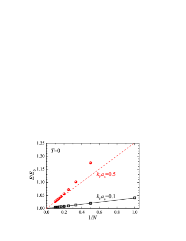
Figure 4: (Color online) The zero-temperature total energy of a quasi-repulsive Fermi gas. The energy is shown in units of the non-interacting energy $E_{0}=(3/5)n\varepsilon_{F}$, as a function of $1/N$ at two interaction parameters: $k_{F}a_{s}=0.1$ (empty squares) and $k_{F}a_{s}=0.5$ (solid circles). The lines are the contribution from the linear part.

In Fig. 4, we show the $1/N$-dependence of the energy of an upper branch Fermi gas at two interaction strengths. At weak interactions ($k_{F}a_{s}=0.1$), the dependence is essentially linear and the use of the leading $1/N$ term is reasonable. For strong interaction strengths ($k_{F}a_{s}=0.5$), the dependence is highly non-linear, due to the unrealistic account of high-order pair fluctuations. In this case, it is physical to keep only the leading linear term of the order $1/N$. The higher-order pair fluctuations should be taken into account by organizing more diagrams beyond Gaussian fluctuations (i.e., the single bosonic loop) and going to the next-to-next-to-leading order $O(1/N^{2})$.

II.3 Dimensional $\epsilon$ expansion

The dimensional $\epsilon$-expansion theory is another non-perturbative theory developed by Nishida and Son for strongly interacting unitary Fermi gases Nishida2006 ; Nishida2007a ; Nishida2007b . This approach is based on an expansion around four or two spatial dimensions, where the pair propagator (or Green function) of Cooper pairs is shown to be a small quantity Nishida2007a . Therefore, one may use the small number $\epsilon=4-d$ (near four spatial dimensions) or $\bar{\epsilon}=d-2$ (near two spatial dimensions) as a parameter to control the perturbation expansion. It was found that even at $\epsilon=1$ and $\bar{\epsilon}=1$ the expansion series is reasonably well-behaved, suggesting that it would be practically useful. Indeed, the next-to-leading-order (NLO) expansion of a unitary Fermi gas already leads to a surprisingly accurate Bertsch parameter at zero temperature, $\xi_{\rm{NLO}}=0.377\pm 0.014$ Nishida2009 , which is very close to the most recent experimental result $\xi=0.376\pm 0.005$ Ku2012 and quantum Monte Carlo result $\xi=0.37-0.38$ Forbes2011 ; Carlson2011 . The predicted superfluid transition temperature $(T_{c}/T_{F})_{\rm{NLO}}=0.183\pm 0.014$ Nishida2007b also agrees very well with the measurement $T_{c}/T_{F}=0.167\pm 0.013$ Ku2012 . For the attractive unitary Fermi gas, one advantage of the dimensional $\epsilon$ expansion is that the Padé (or Borel-Padé) approximation can be employed to match the expansions around four and two spatial dimensions and therefore improves the series summations Nishida2007a ; Nishida2007b ; Nishida2009 ; Arnold2007 .

However, at finite temperature so far the $\epsilon$ expansion theory has only been implemented right at the superfluid transition temperature $T_{c}$. We have re-formulated the $\epsilon$ expansion theory by using the functional path-integral approach and have made the numerical calculations practically easy at finite temperature Mulkerin2016 . In Fig. 5, we compare the $\epsilon$ expansion results (extrapolated from $d=4$) for the universal energy $E(T/T_{F})$ of a ground state unitary Fermi gas with the experimental measurement reported by the MIT group Ku2012 . The agreement is impressively good. This is consistent with the excellent agreement found earlier at zero temperature and at the superfluid transition temperature. All these agreements strongly suggest that the picture of the unitary Fermi gas as a mixture of weakly interacting fermionic and bosonic quasi-particles - which is true near four or two spatial dimensions - could also be a useful starting point even in three spatial dimensions.

Given the fact that there are no phase transitions by changing the dimensionality of the system between $d=4$ and $d=2$, we hope the predictive power of the $\epsilon$ expansion theory may persist as well for a unitary Fermi gas in its quasi-repulsive branch. We note that in the context of statistical physics, the dimensional $\epsilon$ expansion has been extremely successful and has been applied to describe the continuous phase transition close to a critical point Brezin1973 ; Ma1974 ; Moshe2003 .

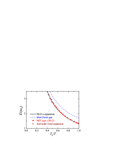
Figure 5: (Color online) Temperature dependence of the total energy of a unitary Fermi gas predicted by the dimensional $\epsilon$ expansion theory. As in Fig. 3, the next-to-leading-order (NLO) $\epsilon$ expansion results (solid line) are contrasted with the MIT data (solid circles), as well as the second-order virial expansion (empty squares).

III Results and discussion

We have performed numerical calculations for arbitrary coupling strength $k_{F}a_{s}>0$ and temperature $T$. For strong coupling at low temperature, the contribution $\Delta\mathcal{P}$ becomes very significant and highly nonlinear. However, our calculations are still controllable with the choice of a large $N$ or a dimensionality of space close to $d=4$. For the large-$N$ expansion, typically, we solve the chemical potential $\mu$ self-consistently by using the number equation $n=\partial\mathcal{P}/\partial\mu$ for $N=50-100$, where $n=Nk_{F}^{3}/(3\pi^{2})$ is the number density. Then, we use the large-$N$ expansion $\mu(N)=\mu_{0}+\mu_{1}/N+o(1/N)$ around the non-interacting chemical potential $\mu_{0}$ to extract the first nontrivial correction $\mu_{1}$ due to pair fluctuations. The final extrapolation to the $N=1$ limit leads to $\mu=\mu_{0}+\mu_{1}$. We apply similar expansions to the total energy, inverse compressibility and inverse spin susceptibility.

Figure 6 reports the interaction parameter dependence of the energy and inverse spin susceptibility at $T=0$ from the large-$N$ expansion. We find that at weak coupling our large-$N$ expansion results are consistent with the predictions from second-order perturbation theory Galitskii1958 . However, there is an apparent deviation when the interaction parameter $k_{F}a_{s}>0.4$. It is impressive that our results agree well with the latest QMC simulations that use different interaction potentials Pilati2010 ; Chang2011 . In particular, for the inverse spin susceptibility, the agreement between the large-$N$ expansion and the QMC data for the hard-sphere potential is exceptionally good. Thus, we determine that at $T=0$ there is a Stoner ferromagnetic transition occurring at $(k_{F}a_{s})_{c}\simeq 0.79$, close to the QMC prediction Pilati2010 .

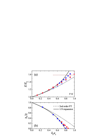
Figure 6: (Color online) The zero-temperature large-$N$ results for the energy (a) and spin susceptibility (b) of a repulsively interacting Fermi gas as functions of the interaction parameter $k_{F}a_{s}$, normalized by the non-interacting results at $T=0$ $E_{0}=(3/5)n\varepsilon_{F}$ and $\chi_{0}=3n/(2\varepsilon_{F})$. For comparison, we also plot the predictions from the second-order perturbation theory (dashed line) and quantum Monte-Carlo simulations (symbols). The blue squares and red circles are the data for the hard-sphere potential and the square-well potential, respectively. The closed symbols are from Ref. Pilati2010 and the open symbols are from Ref. Chang2011 . The dot-dashed horizontal line in (a) is the energy of a fully polarized Fermi gas $E=2^{2/3}E_{0}$.

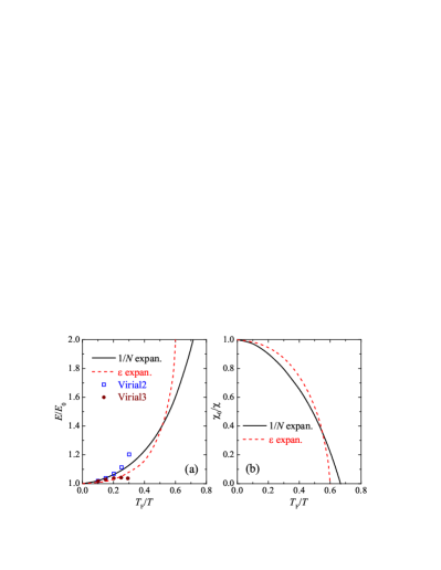
Figure 7: (Color online) The energy (a) and inverse spin susceptibility (b) of a resonantly interacting Fermi gas in the repulsive regime, normalized by the corresponding results of an ideal Fermi gas. In (a), we also show the predictions from the virial expansion theory, up to second or third order.

Figure 7 displays the inverse temperature dependence of the energy and inverse spin susceptibility of a unitary Fermi gas in the quasirepulsive branch. At high temperature, our results reproduce the virial expansion predictions Liu2010a ; Liu2010b ; Ho2004 ; Liu2009 ; Liu2013 , which are the only known results so far for a repulsive unitary Fermi gas. It is interesting that, with decreasing temperature down to $(T_{F}/T)_{c}\simeq 0.6-0.7$ or $T_{c}\simeq 1.5-1.7T_{F}$, both large-$N$ expansion and $\epsilon$ expansion predict a divergent spin susceptibility [see Fig. 7(b)], signifying the phase transition into a Stoner ferromagnetic state. The good agreement between the two different non-perturbative theories strongly indicates that such a transition is realistic and the predicted transition temperature $T_{c}\simeq 1.6T_{F}$ should be qualitatively reliable.

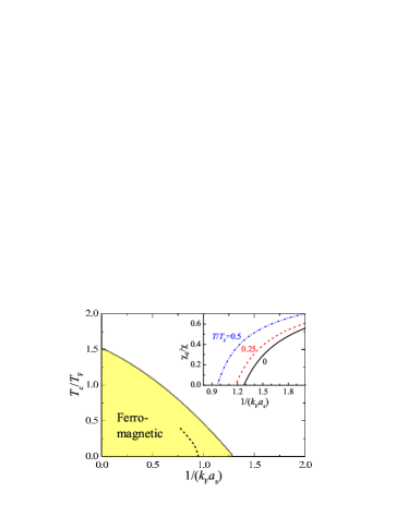
Figure 8: (Color online) Phase diagram of a strongly interacting Fermi gas in its repulsive regime. In the shadow area, the system energetically favors spin-domain formation and exhibits Stoner ferromagnetism. The critical temperature predicted by the second-order perturbation theory in the low-temperature regime is shown by a dashed line. The inset shows the inverse spin susceptibility (normalized by the corresponding non-interacting result) at $T/T_{F}=0$ (solid line), $0.25$ (dashed line), and $0.5$ (dot-dashed line).

We finally show in Fig. 8 a finite temperature phase diagram of the Stoner ferromagnetism. For comparison, we present also the prediction from the second order perturbation theory Duine2005 . At low temperature, it predicts larger critical interaction parameter; while close to the unitary limit, it gives unrealistically high transition temperature due to the strong overestimate of repulsions (not shown in the figure).

It is worth noting that, in all the cases, including the zero temperature in Fig. 6 or the unitary limit in Fig. 7, the compressibility of the quasirepulsive Fermi gas predicted by our theory is always positive. The spin susceptibility is also always well-defined. Therefore, our approach greatly improves the earlier treatments of the quasirepulsive upper branch Shenoy2011 ; Palestini2012 .

In the experimental studies of Stoner ferromagnetism, the Fermi gas was originally prepared with weak interactions and then the interactions were ramped to the strongly repulsive regime. Dynamic rather than adiabatic preparation was used in order to avoid molecule production. In the latest experiment of ⁶Li Fermi gas at temperature $T\sim 0.3T_{F}$, it was found that the rapid decay into bound pairs (molecules) prevents the study of equilibrium phases Sanner2012 . The decay rate can be theoretically estimated by studying the pair formation rate $\Delta$, which is given by the imaginary part of the complex pole of the two-body T-matrix Pekker2011 . At low temperatures ($T<0.5T_{F}$), one finds a large pair formation rate $\Delta>0.1\varepsilon_{F}$ in a wide range of the interaction parameter $k_{F}a_{s}$ Pekker2011 , consistent with the experimental observation of a rapid decay into bound pairs over times on the order of $10\hbar/\varepsilon_{F}$.

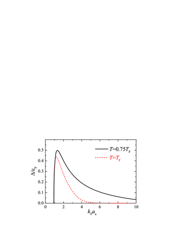
Figure 9: (Color online) The pair formation rate $\Delta$ as a function of the interaction parameter $k_{F}a_{s}$ at $T=0.75T_{F}$ and $T=T_{F}$.

The molecule formation rate can be well estimated by studying the in-medium two-body T-matrix Pekker2011 . The T-matrix is given by the vertex function $\Gamma({\bf q},\omega)$ but with the chemical potential $\mu$ replaced by the one for a noninteracting Fermi gas. The T-matrix normally has a complex pole $\omega({\bf q})=\Omega_{{\bf q}}+i\Delta_{{\bf q}}$, given by the equation $\Gamma^{-1}({\bf q},\omega({\bf q}))=0$. The imaginary part $\Delta_{{\bf q}}$ characterizes the growth rate of pair formation in these quenched experiments. For equal spin populations, the maximal pair formation rate occurs at ${\bf q}=0$. The maximum pair formation rate $\Delta\equiv\Delta_{{\bf q}=0}$ is determined by solving the complex pole from the following equation:

$$\frac{1}{a_{s}}-\sqrt{-mE}-\frac{8\pi}{m}\sum_{\mathbf{k}}\frac{f(\xi_{{\bf k}})}{E-2\varepsilon_{\mathbf{k}}}=0.$$ (40)

In Fig. 9, we examine the pair formation rate at higher temperatures $T=0.75T_{F}$ and $T=T_{F}$. At large $k_{F}a_{s}$, the rate is sensitive to the temperature effect. In particular, in the nondegenerate temperature regime $T\sim T_{F}$, the pair formation rate becomes vanishingly small for large $k_{F}a_{s}$. In this regime, it is possible to study the equilibrium phases of strongly repulsive fermions since the pair formation occurs on a very long time scale $\gg 10\hbar/\varepsilon_{F}$. Therefore, our phase diagram Fig. 8 suggests a promising and realistic way to observe Stoner ferromagnetism at high temperature and at large interaction parameter $k_{F}a_{s}$.

IV Summary

In summary, we have presented a nonperturbative theoretical approach to the quasirepulsive upper branch of a Fermi gas near a broad Feshbach resonance, and we determined the finite-temperature phase diagram for the Stoner instability. One crucial component of our finite-temperature theory is an appropriate definition of a many-body phase shift for the quasirepulsive upper branch. We proved this prescription by resumming the two-body virial contributions from the scattering continuum to infinite order in the fugacity. Our results agree well with the known quantum Monte Carlo simulations at zero temperature, and we recover the known virial expansion prediction at high temperature for arbitrary interaction strengths. At resonance, the predicted Stoner transition temperature becomes of order of the Fermi temperature, around which the molecule formation rate becomes vanishingly small. This suggests a feasible way to avoid the pairing instability and observe Stoner ferromagnetism in strongly interacting atomic Fermi gases.

Note Added. Recently, we became aware of an experimental work Roati2016 that reported the evidence for ferromagnetic instability in the same system as studied in this paper. In that work, the detrimental pairing instability was drastically limited by preparing the gas in a magnetic domain-wall configuration. The ferromagnetic instability was revealed by observing the softening of the spin-dipole collective mode that is linked to the increase of the spin susceptibility. The temperature-coupling phase diagram was determined Roati2016 . Our predictions of the critical gas parameter at $T=0$ [$(k_{F}a)_{c}=0.79$] and the critical temperature around resonance ($\sim T_{F}$) agrees with their experimental measurements.

Appendix A Comparison with the excluded-molecular-pole approximation

The concept of an upper branch is well-defined for a two-particle system, where the whole energy spectrum can be solved precisely Pricoupenko2004 ; Liu2010a . For many-particle systems, however, an unambiguous definition of an upper branch has yet to be established. Indeed, even for three fermions, the identification of the upper-branch energy levels turns out to be difficult Liu2010a . To the best of our knowledge, the quasi-repulsive upper branch of an interacting Fermi gas (at zero temperature) was first mentioned by Pricoupenko and Castin Pricoupenko2004 , when they used a lowest-order constraint variational approach to understand a strongly interacting Fermi gas at the BEC-BCS crossover. The upper branch prescription provided in this work is a useful extension of their idea. As a concrete example, in Fig. 10 we show the total energy of the upper branch and the ground-state branch at a finite temperature $T=3T_{F}$. The generic behavior is not sensitive to the temperature. The use of the temperature $T=3T_{F}$ makes it convenient for us to compare with the result from another approach Shenoy2011 . For the upper branch, in the BEC limit, the Fermi cloud has a weak repulsion and its energy approaches the ideal-gas result as $a_{s}\rightarrow 0^{+}$. In the unitary limit with a divergent scattering length, the energy saturates to a finite value that depends on the temperature.

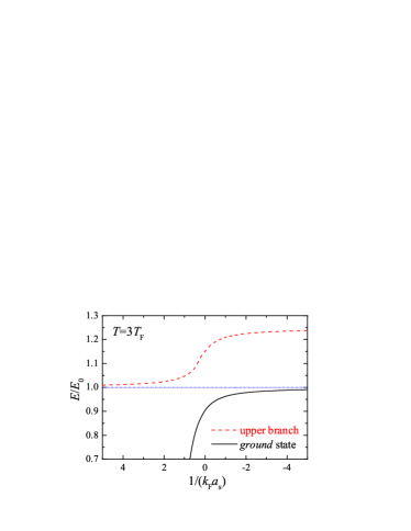
Figure 10: (Color online). The total energy of the upper branch (dashed line) and of the attractive ground state (solid line) at $T=3T_{F}$, measured in units of the energy of an ideal, non-interacting Fermi gas.

In an earlier work Shenoy2011 , Shenoy and Ho proposed a different prescription, the so-called excluded-molecular-pole approximation (EMPA), for the quasirepulsive upper branch of a strongly interacting Fermi gas. An important feature of the EMPA is that it predicts an equilibrium branch-switching phenomenon: The energy of the upper branch reaches a maximum when approaching the resonance from the BEC side and then changes continuously into the lower branch at the BCS side. Here we shall compare the EMPA with our approach.

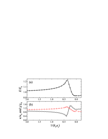
Figure 11: (Color online) The energy, spin susceptibility, and compressibility as functions of the interaction parameter $1/(k_{F}a_{s})$ at $T=3T_{{\rm F}}$ calculated by starting from the pressure (47) with a simple phase shift $\delta_{1}({\bf q},\omega)$ given by (44). The results are consistent with those reported in Shenoy2011 .

A key point of the EMPA is that it starts from the number equation. In the EMPA, the number density due to two-body interaction is given by

$$n_{{\rm rep}}^{(2)}(T,\mu)=\sum_{{\bf q}}\int_{\omega_{s}({\bf q})}^{\infty}\frac{d\omega}{\pi}b(\omega)\frac{\partial\delta({\bf q},\omega)}{\partial\mu},$$ (41)

where the phase shift is defined as

$$\delta({\bf q},\omega)=-{\rm Im}{\rm ln}\left[A({\bf q},\omega)+iB({\bf q},\omega)\right].$$ (42)

The functions $A$ and $B$ are given in Eq. (16). We notice that the ambiguity of the phase shift $\delta({\bf q},\omega)$ is avoided in the above number equation, since it contains only the derivative of the phase shift with respect to the chemical potential. In practice, they use the function ${\rm atan}2(y,x)$ Atan2 ; Shenoyp to evaluate the phase shift and its derivative. Then the two-body contribution to the pressure can be obtained by using the integration method,

$${\cal P}_{{\rm rep}}^{(2)}(T,\mu)=\int_{-\infty}^{\mu}d\mu^{\prime}n_{{\rm rep}}^{(2)}(T,\mu^{\prime}).$$ (43)

To compare the EMPA with our prescription, it is convenient to convert it to an alternative form that starts from the pressure. Toward that end, we first define a simple phase function

$$\delta_{1}({\bf q},\omega)=-\arctan\left[\frac{B({\bf q},\omega)}{A({\bf q},\omega)}\right].$$ (44)

Here $\arctan(x)$ is the usual inverse tangent function with a range $(-\pi/2,\pi/2)$. We have

$$\frac{\partial\delta({\bf q},\omega)}{\partial\mu}=\frac{\partial\delta_{1}({\bf q},\omega)}{\partial\mu}$$ (45)

for $\omega>\omega_{s}({\bf q})$. Hence the number equation of the EMPA can also be expressed as

$$n_{{\rm rep}}^{(2)}(T,\mu)=\sum_{{\bf q}}\int_{\omega_{s}({\bf q})}^{\infty}\frac{d\omega}{\pi}b(\omega)\frac{\partial\delta_{1}({\bf q},\omega)}{\partial\mu}.$$ (46)

The corresponding pressure can be expressed as

$${\cal P}_{{\rm rep}}^{(2)}(T,\mu)=\sum_{{\bf q}}\int_{\omega_{s}({\bf q})}^{\infty}\frac{d\omega}{\pi}b(\omega)\delta_{1}({\bf q},\omega).$$ (47)

The proof of the above result is easy. By taking the derivative of the above pressure with respect to $\mu$ and using the property of the phase $\delta_{1}({\bf q},\omega=\omega_{s}({\bf q}))=0$, we obtain the number equation (46) and hence (41). Therefore, the EMPA is equivalent to a scheme starting from the pressure (47) with a simple phase shift given by (44). This conclusion can also be confirmed numerically. In Fig. 11, we show the results of the energy, spin susceptibility, and compressibility at $T=3T_{F}$ calculated by starting from the pressure (47). They are consistent with the results reported in Shenoy2011 .

In our prescription, the two-body contribution to the pressure is given by

$${\cal P}_{{\rm rep}}^{(2)}(T,\mu)=\sum_{{\bf q}}\int_{\omega_{s}({\bf q})}^{\infty}\frac{d\omega}{\pi}b(\omega)\delta_{{\rm rep}}({\bf q},\omega),$$ (48)

where

$$\delta_{\textrm{rep}}\left(\mathbf{q},\omega\right)=\delta_{\textrm{att}}\left(\mathbf{q},\omega\right)-\pi.$$ (49)

Note that the attractive phase shift $\delta_{\textrm{att}}\left(\mathbf{q},\omega\right)$ should be appropriately determined from its definition $\delta_{{\rm att}}({\bf q},\omega)=-{\rm Im}{\rm ln}\left[A({\bf q},\omega)+iB({\bf q},\omega)\right]$ so that it changes smoothly as a function of $\omega$ for $\omega>\omega_{s}({\bf q})$. This ensures that the repulsive phase shift $\delta_{{\rm rep}}({\bf q},\omega)$ is also a smooth function of $\omega$ for $\omega>\omega_{s}({\bf q})$ and, in particular, $\delta_{{\rm rep}}({\bf q},\omega=0)=0$ (see Fig. 3 of the text).

In summary, the choice of the phase shift is a nontrivial issue for a prescription of the upper branch. The EMPA employs the phase shift $\delta_{1}({\bf q},\omega)$ given by (44), while our prescription adopts the phase shift $\delta_{{\rm rep}}({\bf q},\omega)$ given by (49). Note that our prescription for the phase shift can be proven by resumming the two-particle virial series to all orders in the fugacity, as we have shown in the last section. It is interesting that, in the vacuum, both the phase shifts $\delta_{1}({\bf q},\omega)$ and $\delta_{{\rm rep}}({\bf q},\omega)$ recover the repulsive two-body phase shift $\delta_{2{\rm B}}(k)=-\arctan(ka_{s})$ (for $a_{s}>0$) without bound state. On the other hand, we can show that both the EMPA and our prescription can recover correctly the known perturbative equation of state at weak coupling $k_{F}a_{s}\rightarrow 0^{+}$ and the second-order virial equation of state in the high temperature limit. The difference is that, in the EMPA, the upper branch switches to the lower branch near the resonance. At resonance, the EMPA recovers the virial equation of state for the lower branch, while our theory can reach the repulsive unitary limit.

In an early experiment Bourdel2003 , the interaction energy of a strongly interacting Fermi gas was measured by using the expansion properties of a ⁶Li gas. At temperature $T\simeq 0.6T_{{\rm F}}$, it was found that the interaction energy of the repulsive branch suddenly jumps to negative values at magnetic field $B\simeq 720$ G, which lies at the BEC side of the resonance ($k_{F}a_{s}\sim 1$). This may be an experimental support for the EMPA which predicts an equilibrium switch between the upper and the lower branches. However, to our knowledge, another reasonable explanation for the sudden jump of the interaction energy at $B\simeq 720$ G is the severe nonequilibrium atom loss due to three-body recombination Sanner2012 ; Bourdel2003 ; Massignan2014 . We believe that, once the atom loss rate can be suppressed by some effects (such as high temperature, narrow resonance, mass imbalance, and low dimensionality), one can reach the repulsive unitary limit experimentally.

References

- (1) I. Bloch , J. Dalibard, and W. Zwerger, Many-body physics with ultracold gases, Rev. Mod. Phys. 80, 885 (2008).
- (2) S. Giorgini, L. P. Pitaevskii, and S. Stringari, Theory of ultracold atomic Fermi gases, Rev. Mod. Phys. 80, 1215 (2008).
- (3) E. Stoner, Atomic moments in ferromagnetic metals and alloys with nonferromagnetic elements, Philos. Mag. 15, 1018 (1933).
- (4) P. Massignan, M. Zaccanti, G. M. Bruun, Polarons, dressed molecules, and itinerant ferromagnetism in ultracold Fermi gases, Rep. Prog. Phys. 77, 034401 (2014).
- (5) D. Pekker, M. Babadi, R. Sensarma, N. Zinner, L. Pollet, M. W. Zwierlein, and E. Demler, Competition between pairing and ferromagnetic instabilities in ultracold Fermi gases near Feshbach resonances, Phys. Rev. Lett. 106, 050402 (2011).
- (6) L. Pricoupenko and Y. Castin, One particle in a box: The simplest model for a Fermi gas in the unitary limit, Phys. Rev. A 69, 051601(R) (2004).
- (7) G.-B. Jo, Y.-R. Lee, J.-H. Choi, C. A. Christensen, T. H. Kim, J. H. Thywissen, D. E. Pritchard, and W. Ketterle, Itinerant ferromagnetism in a Fermi gas of ultracold atoms, Science 325, 1521 (2009).
- (8) C. Sanner, E. J. Su, W. Huang, A. Keshet, J. Gillen, and W. Ketterle, Correlations and pair formation in a repulsively interacting Fermi gas, Phys. Rev. Lett. 108, 240404 (2012).
- (9) C. Kohstall, M. Zaccanti, M. Jag, A. Trenkwalder, P. Massignan, G. M. Bruun, F. Schreck, and R. Grimm, Metastability and coherence of repulsive polarons in a strongly interacting Fermi mixture, Nature (London) 485, 615 (2012).
- (10) M. Koschorreck, D. Pertot, E. Vogt, B. Fröhlich, M. Feld, and M. Köhl, Attractive and repulsive Fermi polarons in two dimensions, Nature (London) 485, 619 (2012).
- (11) Duine R. A. & MacDonald A. H. Itinerant ferromagnetism in an ultracold atom Fermi gas Phys. Rev. Lett. 95, 230403 (2005).
- (12) LeBlanc L. J., Thywissen J. H., Burkov A. A. & Paramekanti A. Repulsive Fermi gas in a harmonic trap: Ferromagnetism and spin textures. Phys. Rev. A 80, 013607 (2009).
- (13) H. Zhai, Correlated versus ferromagnetic state in repulsively interacting two-component Fermi gases, Phys. Rev. A 80, 051605(R) (2009).
- (14) G. J. Conduit and B. D. Simons, Repulsive atomic gas in a harmonic trap on the border of itinerant ferromagnetism, Phys. Rev. Lett. 103, 200403 (2009).
- (15) G. J. Conduit, A. G. Green, and B. D. Simons, Inhomogeneous phase formation on the border of itinerant ferromagnetism, Phys. Rev. Lett. 103, 207201 (2009).
- (16) H. Dong, H. Hu, X.-J. Liu, and P. D. Drummond, Mean-field study of itinerant ferromagnetism in trapped ultracold Fermi gases: Beyond the local-density approximation, Phys. Rev. A 82, 013627 (2010).
- (17) X.-J. Liu, H. Hu, and P. D. Drummond, Three attractively interacting fermions in a harmonic trap: Exact solution, ferromagnetism, and high-temperature thermodynamics, Phys. Rev. A 82, 023619 (2010).
- (18) X.-J. Liu and H. Hu, Virial expansion for a strongly correlated Fermi gas with imbalanced spin populations, Phys. Rev. A 82, 043626 (2010).
- (19) S. Zhang, H. H. Hung, and C. Wu, Proposed realization of itinerant ferromagnetism in optical lattices, Phys. Rev. A 82, 053618 (2010).
- (20) Y. Li, E. H. Lieb, and C. Wu, Exact results on itinerant ferromagnetism in multi-orbital systems on square and cubic lattices, Phys. Rev. Lett. 112, 217201 (2014).
- (21) S. Pilati, G. Bertaina, S. Giorgini, and M. Troyer, Itinerant ferromagnetism of a repulsive atomic Fermi gas: A quantum Monte Carlo study, Phys. Rev. Lett. 105, 030405 (2010).
- (22) S. Y. Chang, M. Randeria, and N. Trivedi, Ferromagnetism in repulsive Fermi gases: Upper branch of Feshbach resonance versus hard spheres, Proc. Natl. Acad. Sci. (USA) 108, 51 (2011).
- (23) H. Heiselberg, Itinerant ferromagnetism in ultracold Fermi gases, Phys. Rev. A 83, 053635 (2011).
- (24) L. He and X.-G. Huang, Nonperturbative effects on the ferromagnetic transition in repulsive Fermi gases, Phys. Rev. A 85, 043624 (2012).
- (25) L. He, Finite range and upper branch effects on itinerant ferromagnetism in repulsive Fermi gases: Bethe-Goldstone ladder resummation approach, Ann. Phys. (NY) 351, 477 (2014).
- (26) L. He, Interaction energy and itinerant ferromagnetism in a strongly interacting Fermi gas in the absence of molecule formation, Phys. Rev. A90, 053633 (2014).
- (27) F. Arias de Saavedra, F. Mazzanti, J. Boronat, and A. Polls, Ferromagnetic transition of a two-component Fermi gas of hard spheres, Phys. Rev. A 85, 033615 (2012).
- (28) X. Cui and T.-L. Ho, Phase separation in mixtures of repulsive Fermi gases driven by mass difference, Phys. Rev. Lett. 110, 165302 (2013).
- (29) P. Massignan, Z. Yu, and G. M. Bruun, Itinerant ferromagnetism in a polarized two-component Fermi gas, Phys. Rev. Lett. 110, 230401 (2013).
- (30) P. Nikolić and S. Sachdev, Renormalization-group fixed points, universal phase diagram, and expansion for quantum liquids with interactions near the unitarity limit, Phys. Rev. A 75, 033608 (2007).
- (31) M. Y. Veillette, D. E. Sheehy, and L. Radzihovsky, Large- expansion for unitary superfluid Fermi gases, Phys. Rev. A 75, 043614 (2007).
- (32) T. Enss, Quantum critical transport in the unitary Fermi gas, Phys. Rev. A 86, 013616 (2012).
- (33) Y. Nishida and D. T. Son, expansion for a Fermi gas at infinite scattering length, Phys. Rev. Lett. 97, 050403 (2006).
- (34) Y. Nishida and D. T. Son, Fermi gas near unitarity around four and two spatial dimensions Phys. Rev. A 75, 063617 (2007).
- (35) Y. Nishida, Unitary Fermi gas at finite temperature in the expansion, Phys. Rev. A 75, 063618 (2007).
- (36) X.-J. Liu, B. Mulkerin, L. He, and H. Hu, Equation of state and contact of a strongly interacting Bose gas in the normal state, Phys. Rev. A 91, 043631 (2015).
- (37) M. Rossi, L. Salasnich, F. Ancilotto, and F. Toigo, Monte Carlo simulations of the unitary Bose gas, Phys. Rev. A 89, 041602(R) (2014).
- (38) T. Comparin and W. Krauth, Momentum distribution in the unitary Bose gas from first principles, arXiv: 1604.08870 (2016).
- (39) V. B. Shenoy and T.-L. Ho, Nature and properties of a repulsive Fermi gas in the upper branch of the energy spectrum, Phys. Rev. Lett. 107, 210401 (2011).
- (40) F. Palestini, P. Pieri, and G. C. Strinati, Density and spin response of a strongly interacting Fermi gas in the attractive and quasirepulsive regime, Phys. Rev. Lett. 108, 080401 (2012).
- (41) P. Nozieres and S. Schmitt-Rink, Bose condensation in an attractive fermion gas: From weak to strong coupling superconductivity, J. Low Temp. Phys. 59, 195 (1985).
- (42) C. A. R. Sade Melo, M. Randeria, and J. R. Engelbrecht, Crossover from BCS to Bose superconductivity: Transition temperature and time-dependent Ginzburg-Landau theory, Phys. Rev. Lett. 71, 3202 (1993).
- (43) H. Hu, X.-J. Liu, and P. D. Drummond, Equation of state of a superfluid Fermi gas in the BCS-BEC crossover, Europhys. Lett. 74, 574 (2006).
- (44) X.-J. Liu and H. Hu, BCS-BEC crossover in an asymmetric two-component Fermi gas, Europhys. Lett. 75, 364 (2006).
- (45) M. J. H. Ku, A. T. Sommer, L. W. Cheuk, and M. W. Zwierlein, Revealing the superfluid lambda transition in the universal thermodynamics of a unitary Fermi gas, Science 335, 563 (2012).
- (46) M. M. Forbes, S. Gandolfi, and A. Gezerlis, Resonantly interacting fermions in a box, Phys. Rev. Lett. 106, 235303 (2011).
- (47) J. Carlson, S. Gandolfi, K. E. Schmidt, and S. Zhang, Auxiliary-field quantum Monte Carlo method for strongly paired fermions, Phys. Rev. A84, 061602(R) (2011).
- (48) X.-J. Liu, Virial expansion for a strongly correlated Fermi system and its application to ultracold atomic Fermi gases, Phys. Rep. 524, 37 (2013).
- (49) S. Tan, Energetics of a strongly correlated Fermi gas, Ann. Phys. (NY) 323, 2952 (2008).
- (50) S. Tan, Large momentum part of a strongly correlated Fermi gas, Ann. Phys. (NY) 323, 2971 (2008).
- (51) Y. Nishida, Ground-state energy of the unitary Fermi gas from the expansion, Phys. Rev. A 79, 013627 (2009).
- (52) P. Arnold, J. E. Drut, and D. T. Son, Next-to-next-to-leading-order expansion for a Fermi gas at infinite scattering length, Phys. Rev. A 75, 043605 (2007).
- (53) B. C. Mulkerin, X.-J. Liu, and H. Hu, Beyond Gaussian pair fluctuation theory for strongly interacting Fermi gases, arXiv: 1602.07391 (2016).
- (54) E. Brezin and D. J. Wallace, Critical behavior of a classical Heisenberg ferromagnet with many degrees of freedom, Phys. Rev. B 7, 1967 (1973).
- (55) S. K. Ma, Scaling variables and dimensions, Phys. Rev. A 10, 1818 (1974).
- (56) M. Moshe and J. Zinn-Justin, Quantum field theory in the large N limit: A review, Phys. Rep. 385, 69 (2003).
- (57) V. M. Galitskii, The energy spectrum of a non-ideal Fermi gas, Sov. Phys. JETP 7, 104 (1958).
- (58) T.-L. Ho and E. J. Mueller, High temperature expansion applied to fermions near Feshbach resonance, Phys. Rev. Lett. 92, 160404 (2004).
- (59) X.-J. Liu, H. Hu, and P. D. Drummond, Virial expansion for a strongly correlated Fermi gas, Phys. Rev. Lett. 102, 160401 (2009).
- (60) For the definition of the function , see http://en.wikipedia.org/wiki/Atan2.
- (61) V. B. Shenoy and T.-L. Ho (private communications).
- (62) T. Bourdel, J. Cubizolles, L. Khaykovich, K. M. F. Magalhaes, S. J. J. M. F. Kokkelmans, G. V. Shlyapnikov, and C. Salomon, Measurement of the interaction energy near a Feshbach resonance in a 6Li Fermi gas Phys. Rev. Lett. 91, 020402 (2003).
- (63) G. Valtolina, F. Scazza, A. Amico, A. Burchianti, A. Recati, T. Enss, M. Inguscio, M. Zaccanti, and G. Roati, Evidence for ferromagnetic instability in a repulsive Fermi gas of ultracold atoms, arXiv: 1605.07850 (2016).