Abstract

Next generation of cellular networks deploying wireless distributed femtocaching infrastructure proposed by Golrezaei et. al. are studied. By taking advantage of multihop communications in each cell, the number of required femtocaching helpers is significantly reduced. This reduction is achieved by using the underutilized storage and communication capabilities in the User Terminals (UTs), which results in reducing the deployment costs of distributed femtocaches.

A multihop index coding technique is proposed to code the cached contents in helpers to achieve order optimal capacity gains. As an example, we consider a wireless cellular system in which contents have a popularity distribution and demonstrate that our approach can replace many unicast communications with multicast communication. We will prove that simple heuristic linear index code algorithms based on graph coloring can achieve order optimal capacity under Zipfian content popularity distribution.

Multihop Caching-Aided Coded Multicasting for the Next Generation of Cellular Networks

Mohsen Karimzadeh Kiskani^†, and Hamid R. Sadjadpour^†, Copyright (c) 2015 IEEE. Personal use of this material is permitted. However, permission to use this material for any other purposes must be obtained from the IEEE by sending a request to pubs-permissions@ieee.org. M. K. Kiskani^† and H. R. Sadjadpour^† are with the Department of Electrical Engineering, University of California, Santa Cruz. Email: {mohsen, hamid}@soe.ucsc.edu

I Introduction

With the recent pervasive surge in using wireless devices for video and high speed data transfer, it seems eminent that the current wireless cellular networks cannot be a robust solution to the ever-increasing wireless bandwidth utilization demand. Researchers have been recently focused on laying down the fundamental grounds for future cellular networks to overcome such problems.

Deploying home size base stations is proposed as a solution in [7]. The solution in [7] is based on the idea of femtocells in which many small cells are deployed throughout the network to cover the entire network. Deploying many small cells in the network with reliable backhaul links requires significant capital investment. Therefore, Golrezaei et. al. [14] proposed femtocaching as an alterante solution to overcome this problem. In this approach, in every cell along with the main base station, smaller base stations with low-bandwidth backhaul links and high storage capabilities are deployed to create a wireless distributed caching infrastructure. These small base stations which are called caching helpers (or simply helpers), will store popular contents in their caches and use their caches to serve User Terminal (UT) requests. Therefore, in networks with high content reuse, the backhaul utilization will be significantly reduced using this approach. If the requested content is not available in the helper’s cache, UTs can still download the content from their low-bandwidth backhaul links to the base station. The proposed technique in [14] requires deployment of large number of femtocaches in order to cover all the nodes in the network.

On the other hand, it is well-known that web content request popularity follows Zipfian-like distributions [6]. This content popularity distribution implies that few popular contents are widely requested by the network UTs. We assume UTs store their requested contents and therefore, helpers can multicast multiple requests by taking advantage of coding to reduce the total number of transmissions.

In this paper, we propose to use index coding to code the contents in helpers before transmission. Index coding is a source coding technique proposed in [3] which takes advantage of UTs’ side information in broadcast channels to minimize the required number of transmissions. In index coding, the source (e.g. base station) designs codes based on the side information stored in requesting nodes. The coded information is broadcasted to the UTs that use the information together with their cached contents to decode the desired content. Index coding improves bandwidth utilization by minimizing the number of required transmissions. We propose to extend index coding approach from broadcast one-hop communication to multihop scenarios which will be explained in details.

Our main motivation to use index coding is the high storage availability in UTs to improve the achievable throughput of the future wireless cellular networks. Current improvements in high density storage systems has made it possible to have personal devices with Terabytes of storage capability. This ever-increasing trend provides future personal wireless devices with huge under-utilized storage capabilities. Future wireless devices can use their storage capability to store the contents that they have already requested. In an index coding setting, many UTs that are requesting different contents can receive a coded file which is multicasted to them and then each UT uses the information in its cache to decode its requested content from the received coded file. There is an important equivalence between index coding and network coding as stated in [11, 10] and therefore, the results in this paper can also be stated based on a network coding terminology.

We will prove that index coding can be efficiently used to encode the contents by helpers under a Zipfian distribution model. The encoded contents can be relayed through multiple hops to all the UTs being served by that helper.

The optimal index coding solution is an NP-Hard problem [18]. However, we will show that even using linear index codes can result in order optimal capacity gains in these networks. We believe that this coding technique can serve as a complement to the solution proposed in [14]. As clearly articulated in [21], in any caching problem we are faced with two phases of cache placement and cache delivery. While [14] proposes efficient cache placement algorithms, we will be focusing on efficient delivery methods for their solution. We will show that the problem of delivery in [14] can be efficiently addressed by using index coding in the helpers.

Recent discussions on standards for future 5G cellular networks are focused on providing high bandwidth for Device-to-Device communications (D2D). Examples of such approaches are the IEEE 802.11ad standard (up to 60GHz [2]) and the millimeter-wave proposal which can potentially enable up to 300GHz of bandwidth for D2D communications [4, 1]. This potential abundant D2D bandwidth can be utilized to relay the coded contents inside an ad hoc network which is being served by a helper. It is indeed such excessive storage and bandwidth capabilities of future wireless systems that make our solution feasible.

Deploying many femtocaching helpers is not economically efficent. On the other hand, since UTs have significant D2D capabilities, they can efficiently participate in content delivery through multihop D2D communications. In our proposal, we suggest to deploy few helpers which can deliver the contents to neighboring UTs through multihop D2D communications. This can reduce the network deployment and maintenance costs.

The rest of this paper is organized as follows. Section II reviews the related works and section III describes the proposed network model that is similar to [14] with the addition of using multihop communications and index coding. In section IV, we will explain the scaling laws of capacity improvement using index coding and relaying. Section V demonstrates that index coding algorithms can achieve order optimal gains. Section VI describes the simulation results and the paper is concluded in section VII.

II Related work

The problem of caching when a server is transmitting contents to clients was studied in [21] from an information theoretic point of view. The authors introduced two phases of cache placement and content delivery. For a femtocaching solution, efficient cache placement algorithms are proposed in [14]. In this paper, we focus on efficient content delivery algorithms through index coding and multihop D2D communications for a femtocaching solution.

There has been significant research on index coding since it was proposed in [3]. The practical implementation of index coding for wireless applications was proposed in [8] by proposing cycle counting methods. A dynamic index coding solution for wireless broadcast channels is proposed in [23]. In [23], a wireless broadcast station is considered and a simple set of codes based on cycles in the dependency graph is provided. They show the optimality of these codes for a class of broadcast relay problems. In this paper, we prove that codes based on cycles can acheive order optimal capacity gains in networks with Zipfian content request distribution.

Approximating index coding solution is proved [3] to be an NP-Hard problem. However, efficient heuristics has been proposed in [9] which are based on well-known graph coloring algorithms. Other references like [11] and [10] have studied the connections and equivalence between index coding and network coding. Tran et al. [24] studied a single hop wireless link from a network coding approach and showed similar results to index coding. Ji et al. [16] studied theoretical limits of caching in D2D communication networks.

Study of coding techniques in networks with high content reuse has recently attracted the attention of researchers. Montpetit et al. [22] studied the applications of network coding in Information-Centric Networks (ICN). Wu et al. [25] studied network coding in Content Centric Networks (CCN) which is an implementation of ICN. Leong et al. [19] proposed a linear programming formulation to deliver contents optimally in today’s IP based Content Delivery Networks (CDN) using network coding. Llorca et at. [20] proposed a network-coded caching-aided multicasting technique for efficient content delivery in CDNs. This paper extends Index Coding to multihop communication and shows that linear codes can achieve order optimal capacity gains in such networks.

III Network Model

We assume a network model for future wireless cellular networks in which femtocaching helpers with significant storage capabilities are deployed throughout the network to assist the efficient delivery of contents to UTs through reliable D2D communications. Such helpers are characterized with low rate backhaul links which can be wired or wireless. They will also have localized, high-bandwidth communication capabilities. With their significant storage capacity, in a network with high content reuse, many of the content requests for the UTs inside a cell can be satisfied directly by the helpers.

Each helper is serving a wireless ad-hoc network in which the UTs are utilizing high bandwidth D2D communication techniques such as millimeter wave and IEEE 802.11ad technologies. This high bandwidth D2D communication enables the UTs to relay data from a nearby helper to all the UTs that are within transmission range. We assume that the path lifetime between the helper and UTs is longer than the time required to transmit the content. For large files and when UTs are moving fast, one solution is to divide the content into smaller files and treat each file separately. The paper assumes that the network is connected which can be justified by the large number of UTs that will be available in the future wireless cellular networks.

Further, we take advantage of index coding and the side information cached in UTs to significantly reduce the required number of helpers and consequently, reduce the infrastructure maintenance and deployment costs. To demonstrate the effectiveness of using multihop communications, we consider similar assumptions as [14] with a macro base station placed in the center of a cell with radius 400 meters serving 1000 UTs and a transmission range of 100 meters [1] for D2D communication. As shown in Figure 1, with only 4 helpers uniformly located in the cell, 100% and 80% of nodes are covered with 3 and 2 hop communications respectively. Covering all the UTs in the same cell with only one hop communication requires up to 27 helpers [14].

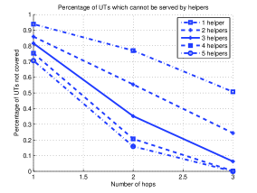
Figure 1: Pertentage of UTs not covered versus the maximum number of hops traveled. This simulation is carried over a cell with radius 400 meters and with a communication range of 100 meters.

Clearly, for a vehicle or a mobile UT operating in the cell, the handover probability will be significantly reduced if the number of helpers shrinks from 27 to 4.

We assume that $n$ UTs denoted by $\mathbb{N}=\{N_{1},N_{2},...,N_{n}\}$ are being served by a helper. There are $m$ contents $\mathbb{M}=\{M_{1},M_{2},...,M_{m}\}$ available with $M_{1}$ as the most popular content and $M_{m}$ as the least popular content in the network . Let’s assume UT $N_{i}$ requests a content with popularity index $r_{i}$ in the current time interval. Each UT has a cache of fixed size $\delta$ in which contents with indices $C_{i}=\{{c_{i1}},...,{c_{i\delta}}\}$ are stored. Therefore, we assume that UT $N_{i}$ caches contents $M_{{c_{i1}}},M_{{c_{i2}}},\dots,M_{{c_{i\delta}}}$ and the set of cached content indices in $N_{i}$ is represented by $C_{i}$. Therefore, if we denote the set of cached contents in UT $N_{i}$ by $\mathcal{M}_{i}$, then we have $\mathcal{M}_{i}=\{M_{j}~{}|~{}j\in C_{i}\}$. The requested content index is shown by $r_{i}$.

Let’s assume that we have $n$ UTs each with a set of side information $\mathcal{M}_{i}$. The formal definition of index code described in [3] is given below.

Definition 1.

An index code on a set of $n$ UTs each with a side information set $\mathcal{M}_{i}\subseteq\mathbb{M}$, and a requesting content ${M}_{r_{i}}\in\mathbb{M}$ for $i=1,2,\dots,n$ is defined as a set of codewords in $\{0,1\}^{l}$ toghether with

1. An encoding function $\mathcal{E}$ mapping inputs in $\{0,1\}^{m}$ to codewords and

2. A set of decoding functions $\mathcal{D}_{1},\mathcal{D}_{2},\dots,\mathcal{D}_{n}$ such that $\mathcal{D}_{i}(\mathcal{E}(\mathbb{M}),\mathcal{M}_{i})={M}_{r_{i}}$ for $i=1,2,\dots,n$.

In the above definition, the length of the index code $l$ denotes the number of required transmissions to satisfy all the content requests of the $n$ UTs. The encoding function $\mathcal{E}$ is applied to the contents by the helper and the decoding functions $\mathcal{D}_{i}$s are applied individually by UTs to decode their desired contents from the encoded content using their cached information.

Figure 2 shows a helper $H$ serving 6 UTs $N_{1},N_{2},N_{3},N_{4},N_{5},$ and $N_{6}$. Let’s assume UTs $N_{1},N_{2}$ and $N_{5}$ request contents $M_{3},M_{1}$ and $M_{4}$ while storing $\{M_{1},M_{4}\}$, $\{M_{3},M_{4}\}$ and $\{M_{1},M_{3}\}$ respectively. Using index coding requires 3 channel usages while without index coding, we need 5 channel usages. This is true since using index coding, the helper creates the XOR combination of contents $M_{1},M_{3}$ and $M_{4}$ as $M_{1}\oplus M_{3}\oplus M_{4}$ and broadcasts this coded content to its neighboring UTs. Either of $N_{1}$ and $N_{2}$ can immediately reconstruct their requested content from this coded content. For instance, $N_{1}$ which is requesting $M_{3}$ can decode its requested content by using it’s cached information and XOR operation on the encoded message to retrieve the requested content $M_{3}$, i.e., $(M_{1}\oplus M_{3}\oplus M_{4})\oplus M_{1}\oplus M_{4}=M_{3}$. After $N_{2}$ receives $M_{1}\oplus M_{3}\oplus M_{4}$, it relays it to node $N_{4}$ which simply broadcasts it to $N_{5}$. UT $N_{5}$ will again use XOR operation to decode it’s desired content $M_{4}$ by adding it’s cached contents to the coded content that it has received, i.e., $(M_{1}\oplus M_{3}\oplus M_{4})\oplus M_{1}\oplus M_{3}=M_{4}$. Therefore, only 3 transmissions are needed.

To satisfy the content requests through multihop D2D without index coding, 5 transmissions are needed as the helper should transmit $M_{3}$ to $N_{1}$, $M_{1}$ to $N_{2}$, $M_{4}$ to $N_{2}$, and $N_{2}$ relays $M_{4}$ to $N_{4}$ and $N_{4}$ relays it to $N_{5}$.

Figure 2: Example of a wireless multihop network being served by the helper $H$. Each arrow represents a link with high bandwidth D2D communication capability.

We assume a Zipfian distribution with parameter $s>1$ for content popularity distribution in the network. This means that the probability that UT $N_{i}$ requests any content with index $r_{i}$ at any time instant is given by

$$\textrm{Pr}[N_{i}~{}\textrm{requests content with index}~{}r_{i}]=\frac{r_{i}^{-s}}{H_{m,s}},$$ (1)

where $H_{m,s}=\sum_{j=1}^{m}\frac{1}{j^{s}}$ denotes the $m^{th}$ generalized harmonic number with parameter $s$.

Remark 1.

This paper only focuses on Zipfian content request probability with parameter $s>1$ which is a non-heavy-tailed probability distribution. Our results are correct for any type of non-heavy-tailed probability distribution and the extension to heavy-tailed probability distribution is the subject of future work.

Dependency graph is a useful analytical tool [3, 11, 8] that is widely used in index coding literature.

Definition 2.

(Dependency Graph): Given an instance of an index coding problem, the dependency graph $\overrightarrow{G}(V,E)$ is defined as

• each UT $N_{i}$ corresponds to a vertex in $V$, $N_{i}\in V$, and

• there is a directed edge in $E$ from $N_{i}$ to $N_{j}$ if and only if $N_{i}$ is requesting a content that is already cached in $N_{j}$.

This dependency graph does not represent the actual physical links between UTs in the network. This is a virtual graph in which each edge represents the connection between a UT that is requesting a content and a UT that caches this content. As discussed in [8, 23], every cycle in the dependency graph is representative of a connection between UTs and it can save one transmission. For every clique in the dependency graph, all the requesting UTs in the clique can be satisfied by a simple linear XOR index code. The complement of dependency graph is called conflict graph. This graph is of significant interest since any clique in the dependency graph gives rise to an independent set in the conflict graph. Therefore, well-known graph coloring algorithms over conflict graph can be used to find simple linear XOR index codes. The dependency and conflict graphs in our network are random directed graphs. In the next section, we will use the properties of these graphs to find the capacity gains and propose simple index coding solutions.

To prove our results in this paper, we have used Least Recently Used (LRU) or Least Frequently Used (LFU) cache policies. Similar results can be produced for other caching policies. LRU caching policy assumes that most recently requested contents are kept in the cache. In LRU caching, in each time slot the content that is requested in the previous time slot is stored in the first cache location. If this content was already available in the cache, it is moved from that location to the first cache location. If the content was not available, then the content that is least recently used is discarded and the most recently requested content is cached in the first cache location. Any other content is relocated to a new cache location such that the contents appear in the order that they have been requested.

In LFU caching policy, the contents are cached based on their request frequency. Highly popular contents are stored in the first locations of the cache and contents with lower request frequency are cached in the bottom locations of the cache.

Computing the probability of having content with index $r_{i}$ in cache $C_{j}$, $\textrm{Pr}[r_{i}\in C_{j}]$, turns out to be complicated for LRU or LFU caching policies. A simple lower bound on this probability for LRU can be found by noticing that $\textrm{Pr}[r_{i}\in C_{j}]$ is greater than the probability that UT $N_{j}$ have requested the content with index $r_{i}$ in the most recent time slot and therefore it is located at the top of the cache. This lower bound can be derived using equation (1).

$$\textrm{Pr}[r_{i}\in C_{j}] =\textrm{Pr}[c_{j1}=r_{i}]+\sum_{l=2}^{\delta}\textrm{Pr}[c_{jl}=r_{i}]$$

$$\geq\textrm{Pr}[c_{j1}=r_{i}]=\frac{r_{i}^{-s}}{H_{m,s}}.$$ (2)

To prove that the same lower bound holds for LFU, notice that $\textrm{Pr}[r_{i}\in C_{j}]$ is larger than the same probability when the cache size is $M=1$. Therefore,

$$\textrm{Pr}[r_{i}\in C_{j}]\geq\textrm{Pr}[r_{i}\in C_{j}~{}|~{}M=1]=\textrm{Pr}[c_{j1}=r_{i}]=\frac{r_{i}^{-s}}{H_{m,s}}.$$ (3)

In the subsequent sections, we will use these lower bounds to prove our results.

In this paper, we will state our results in terms of order bounds. To avoid any confusion, we use the following order notations [17]. We denote $f(n)=\operatorname{O}(g(n))$ if there exist $c>0$ and $n_{0}>0$ such that $f(n)\leq cg(n)$ for all $n\geq n_{0}$, $f(n)=\Omega(g(n))$ if $g(n)=\operatorname{O}(f(n))$, and $f(n)=\Theta(g(n))$ if $f(n)=\operatorname{O}(g(n))$ and $g(n)=\operatorname{O}(f(n))$.

IV Order optimal capacity gain

In this section, we will prove that index coding can significantly decrease the number of transmissions in the network. We will specifically use the Zipfian content distribution in the underlying content distribution network. To do so, we will first state and prove the following lemma.

Lemma 1.

Let’s consider a Zipfian content distribution with parameter $s>1$ and parameter $h_{\epsilon}={\epsilon}^{\frac{1}{1-s}}$ where $0<\epsilon<1$. For every $i$ with popularity index $r_{i}$ that is less than $h_{\epsilon}$, the request probability is at least $1-\epsilon$.

Proof.

Based on the Zipfian distribution assumption and equation (1), the probability that the requested content has a popularity of at most $h_{\epsilon}$ is equal to

$$\textrm{Pr}[r_{j}\leq h_{\epsilon}]=\frac{H_{h_{\epsilon},s}}{H_{m,s}}.$$ (4)

In order to satisfy $\textrm{Pr}[r_{j}\leq h_{\epsilon}]\geq 1-\epsilon$, we should have

$$\epsilon \geq 1-\textrm{Pr}[r_{j}\leq h_{\epsilon}]=1-\frac{H_{h_{\epsilon},s}}{H_{m,s}}=\dfrac{1}{H_{m,s}}\sum_{j=h_{\epsilon}+1}^{m}j^{-s}$$

$$=\dfrac{1}{H_{m,s}}\sum_{i=1}^{\lfloor\frac{m}{h_{\epsilon}}\rfloor-1}\sum_{j=ih_{\epsilon}+1}^{(i+1)h_{\epsilon}}j^{-s}+\dfrac{1}{H_{m,s}}\sum_{j=\lfloor\frac{m}{h_{\epsilon}}\rfloor h_{\epsilon}+1}^{m}j^{-s}.$$ (5)

If we have

$$\epsilon \geq\dfrac{1}{H_{m,s}}\sum_{i=1}^{\lfloor\frac{m}{h_{\epsilon}}\rfloor}\sum_{j=ih_{\epsilon}+1}^{(i+1)h_{\epsilon}}j^{-s},$$ (6)

then the inequality in (5) will certainly hold since the right hand side in (6) is larger than the right hand side in (5). Note that, for $ih_{\epsilon}+1\leq j\leq(i+1)h_{\epsilon}$ we have $j^{-s}<(ih_{\epsilon})^{-s}$. Hence,

$$\sum_{j=ih_{\epsilon}+1}^{(i+1)h_{\epsilon}}j^{-s}<\sum_{j=ih_{\epsilon}+1}^{(i+1)h_{\epsilon}}(ih_{\epsilon})^{-s}=h_{\epsilon}(ih_{\epsilon})^{-s}=i^{-s}h_{\epsilon}^{1-s}$$ (7)

This means that if

$$\epsilon \geq h_{\epsilon}^{1-s}\dfrac{1}{H_{m,s}}\sum_{i=1}^{\lfloor\frac{m}{h_{\epsilon}}\rfloor}i^{-s},$$ (8)

then (6) holds since the right hand side of inequality (6) is smaller than the right hand side of inequality (8) as shown by (7). Notice that since,

$$\dfrac{1}{H_{m,s}}\sum_{i=1}^{\lfloor\frac{m}{h_{\epsilon}}\rfloor}i^{-s}=\dfrac{\sum_{i=1}^{\lfloor\frac{m}{h_{\epsilon}}\rfloor}i^{-s}}{\sum_{i=1}^{\lfloor\frac{m}{h_{\epsilon}}\rfloor}i^{-s}+\sum_{\lfloor\frac{m}{h_{\epsilon}}\rfloor+1}^{m}i^{-s}}<1,$$

if $h_{\epsilon}$ is chosen such that

$$\epsilon \geq h_{\epsilon}^{1-s},$$ (9)

then all of the inequalities in equations (5), (6), (7) and (8) will be valid and hence $\textrm{Pr}[r_{j}\leq h_{\epsilon}]\geq 1-\epsilon$. Therefore, in order to have $\textrm{Pr}[r_{j}\leq h_{\epsilon}]\geq 1-\epsilon$, it is enough to choose $h_{\epsilon}$ such that (9) is valid. Hence, if $h_{\epsilon}$ is chosen to be at least equal to

$$h_{\epsilon}={\epsilon}^{\frac{1}{1-s}},$$ (10)

then we have $\textrm{Pr}[r_{j}\leq h_{\epsilon}]\geq 1-\epsilon$. Notice that the choice of $h_{\epsilon}$ in (10) is such that it only depends on $\epsilon$ and is independent of $m$. ∎

For instance for $s=2$ and $\epsilon=0.01$, $h_{\epsilon}$ can be chosen as 100 (regardless of the size of $m$). This implies that for a Zipfian distribution with $s=2$, 100 highly popular contents among any large number of contents would account for 99% of the total content requests. Therefore, if $h_{\epsilon}$ is chosen as in equation (10), with a probability of at least $1-\epsilon$ all content requests have popularity index of at most $h_{\epsilon}$. Now define $p_{\epsilon}$ as

$$p_{\epsilon}\triangleq\dfrac{h_{\epsilon}^{-s}}{H_{m,s}}=\dfrac{{\epsilon}^{-\frac{s}{1-s}}}{H_{m,s}}.$$ (11)

Based on above discussion, in our instance of index coding dependency graph, with a probability of at least $1-\epsilon$ edges are present with a probability of at least $p_{\epsilon}$. We will discuss this in more details later in the proof for Theorem 1. Notice that for large values of $m$, $p_{\epsilon}$ is also independent of $m$ since in that case $H_{m,s}\approx\zeta(s)$ and $p_{\epsilon}$ only depends on $\epsilon$ and $s$.

As stated in [8], if we choose the right encoding vectors for any index coding problem, for any vertex disjoint cycle in the dependency graph we can save one transmission. Therefore, the number of vertex-disjoint cycles in the dependency graph can serve as a lower bound for the number of saved transmissions in any index coding problem. Number of vertex disjoint cycles is also used in [23] as a way of finding the lower bound for index coding gain. To count the number of vertex-disjoint cycles in our random dependency graph, we will use the following lemma originally proved as Theorem 1 in [12].

Lemma 2.

Let $d>1$ and $v\geq 24d$ be integers. Then any graph $G^{v}_{f(v,d)}$ with $v$ vertices and at least $f(v,d)=(2d-1)v-2d^{2}+d$ edges contains $d$ disjoint cycles or $2d-1$ vertices of degree $v-1$.

Note that the dependency graph is a directed graph and in order to use Lemma 2, we need to construct an undirected graph. Let’s denote the directed and undirected random graphs on $n$ vertices and edge presence probability $p_{\epsilon}$ by $\overrightarrow{G}(n,p_{\epsilon})$ and ${G}(n,p_{\epsilon})$, respectively. In a directed graph $\overrightarrow{G}(n,p_{\epsilon})$, the probability that two vertices are connected by two opposite directed edges is $p_{\epsilon}^{2}$. Therefore, we can build an undirected graph ${G}(n,p_{\epsilon}^{2})$ with the same number of vertices and an edge between two vertices if there are two opposite directed edges in the directed graph $\overrightarrow{G}(n,p_{\epsilon})$ between these two UTs. Hence, $\overrightarrow{G}(n,p_{\epsilon})$ essentially contains a copy of $G(n,p_{\epsilon}^{2})$. Note that there are some edges between UTs in $\overrightarrow{G}(n,p_{\epsilon})$ that do not appear in $G(n,p_{\epsilon}^{2}).$ This fact was also observed in [15]. Therefore, a lower bound on the number of disjoint cycles for $G(n,p_{\epsilon}^{2})$ implies a lower bound on the number of disjoint cycles for $\overrightarrow{G}(n,p_{\epsilon})$.

In the following theorems, we will use Lemma 2 to prove that using index coding to code the contents can be very efficient.

Theorem 1.

Assume all UTs are utilizing LRU or LFU caching policies for a Zipfian content request distribution with parameter $s>1$. Index coding can save $\Omega(np_{\epsilon}^{2})$ transmissions for any helper serving $n$ UTs with a probability of at least $1-\epsilon$ for any $0<\epsilon<1$.

Proof.

Consider a Zipfian distribution with parameter $s>1$ and let $0<\epsilon<1$ be fixed. The dependency graph $\overrightarrow{G}(V,E)$ in our problem is composed of $n$ vertices $N_{1},N_{2},\dots,N_{n}$ which correspond to the $n$ UTs that are served by a helper. Note that the existence of an edge in dependency graph depends on the probability that a UT is requesting a content and another UT has already cached that content. Therefore, this is a non-deterministic graph with some probability for the existence of each edge between the two vertices. In this non-deterministic dependency graph, the probability of existence of edge $(N_{i},N_{j})$ in $E$ is equal to the probability that content $r_{i}$ requested by $N_{i}$, is already cached in $N_{j}$. Therefore, with LRU or LFU caching policy assumption and using equations (2) and (3), we arrive at

$$\textrm{Pr}[(N_{i},N_{j})\in E]=\textrm{Pr}[r_{i}\in C_{j}]\geq\frac{r_{i}^{-s}}{H_{m,s}}.$$ (12)

Using Lemma 1 for any $0<\epsilon<1$, if $h_{\epsilon}$ is chosen as $h_{\epsilon}={\epsilon}^{\frac{1}{1-s}}$, then with a probability of at least $1-\epsilon$, any requested content has a popularity index $r_{i}$ less than $h_{\epsilon}$. This means that with a probability of at least $1-\epsilon$, the edge presence probability in equation (12) can be lower bounded by $p_{\epsilon}$. Therefore, with a probability of at least $1-\epsilon$, maximum number of vertex-disjoint cycles in our directed dependency graph $\overrightarrow{G}(V,E)$ can be lower bounded by the maximum number of vertex-disjoint cycles in an Erdős-Réyni random graph $\overrightarrow{G}(n,p_{\epsilon})$ with $n$ vertices and edge presence probability $p_{\epsilon}$. Now we can use Lemma 2 and undirected graph ${G}(n,p_{\epsilon}^{2})$ to find a lower bound on the number of vertex disjoint cycles in $\overrightarrow{G}(n,p_{\epsilon})$. This in turn, will give us a lower bound on the number of vertex-disjoint cycles in $\overrightarrow{G}(V,E)$.

Note that $G(n,p_{\epsilon}^{2})$ is an undirected Erdős-Réyni random graph on $n$ vertices and edge presence probability $p_{\epsilon}^{2}$. This graph has a maximum of $n(n-1)$ undirected edges. However, since every undirected edge in this graph exists with a probability of $p_{\epsilon}^{2}$, the expected value of the number of edges in graph $G(n,p_{\epsilon}^{2})$ is $n(n-1)p_{\epsilon}^{2}$. This means that if $d$ in Lemma 2 with $v=n$ is chosen to be an integer such that

$$n(n-1)p_{\epsilon}^{2}\geq(2d-1)n-2d^{2}+d,$$ (13)

then on average, $G(n,p_{\epsilon}^{2})$ will have either $d$ disjoint cycles or $2d-1$ vertices of degree $n-1$. For the purpose of our paper we can easily verify that for large enough values of $n$, $d^{\star}=\lfloor\frac{np_{\epsilon}^{2}}{24}\rfloor$ satisfies equation (13) (Notice that the condition $24d^{\star}\leq n$ in Lemma 2 is also met). Therefore based on Lemma 2, the graph $G(n,p_{\epsilon}^{2})$ either has at least $d^{\star}=\lfloor\frac{np_{\epsilon}^{2}}{24}\rfloor$ disjoint cycles or $2d^{\star}-1=2\lfloor\frac{np_{\epsilon}^{2}}{24}\rfloor-1$ vertices with degree $n-1$. As mentioned before, $\overrightarrow{G}(n,p_{\epsilon})$ essentially contains a copy of $G(n,p_{\epsilon}^{2})$. Consequently, $\overrightarrow{G}(n,p_{\epsilon})$ either has at least $d^{\star}=\lfloor\frac{np_{\epsilon}^{2}}{24}\rfloor$ disjoint cycles or $2d^{\star}-1=2\lfloor\frac{np_{\epsilon}^{2}}{24}\rfloor-1$ vertices with degree $n-1$. The number of vertices in graph $\overrightarrow{G}(n,p_{\epsilon})$ is $n$. Therefore, the latter case gives rise to a situation where there are $2d^{\star}-1=2\lfloor\frac{np_{\epsilon}^{2}}{24}\rfloor-1$ vertices which are connected to any other vertex in $\overrightarrow{G}(n,p_{\epsilon})$ through undirected edges. This condition results in having a clique of size $2\lfloor\frac{np_{\epsilon}^{2}}{24}\rfloor-1$ in $\overrightarrow{G}(n,p_{\epsilon})$.

In summary, $\overrightarrow{G}(n,p_{\epsilon})$ has either $d^{\star}$ disjoint cycles or it contains a clique of size $2d^{\star}-1$. Hence, with a probability of at least $1-\epsilon$, the dependency graph $\overrightarrow{G}(V,E)$ on average has either $d^{\star}$ disjoint cycles or it contains a clique of size $2d^{\star}-1$. In either of these cases $d^{\star}=\lfloor\frac{np_{\epsilon}^{2}}{24}\rfloor$ transmissions can be saved using index coding. This proves the theorem. ∎

Theorem 2.

Index coding through cycle counting and clique partitioning can save $\Theta(n)$ transmissions in a network with $n$ UTs and Zipfian content request distribution with parameter $s>1$.

Proof.

In Theorem 1, we proved that in a network with Zipfian content request distribution and for a fixed $0<\epsilon<1$, with a probability of at least $1-\epsilon$, the index coding dependency graph either has $d^{\star}=\lfloor\frac{np_{\epsilon}^{2}}{24}\rfloor$ disjoint cycles or it contains a clique of size $2d^{\star}-1=2\lfloor\frac{np_{\epsilon}^{2}}{24}\rfloor-1$. Consider the following situations,

1. The dependency graph has $d^{\star}=\lfloor\frac{np_{\epsilon}^{2}}{24}\rfloor$ disjoint cycles. In this case, for a fixed $\epsilon$, $p_{\epsilon}$ is a constant which does not depend on $n$. Hence, cycle counting can result in at least $d^{\star}=\lfloor\frac{np_{\epsilon}^{2}}{24}\rfloor=\Omega(n)$ transmission savings. This is a lower bound on the number of transmission savings.

   On the other hand, notice that the maximum number of vertex-disjoint cycles in any graph with $n$ vertices cannot be greater than $\frac{n}{2}$ as shown in Figure 3. Therefore, the maximum number of transmission savings using cycle counting is $\frac{n}{2}=O(n)$. This is an upper bound on the number of saved transmissions. Since the order of upper and lower bounds are the same, it can be concluded that the number of saved transmissions scales as $\Theta(n)$ .

2. The dependency graph contains a clique of size $\mathrm{k}^{\star}=2d^{\star}-1=2\lfloor\frac{np_{\epsilon}^{2}}{24}\rfloor-1$. Through clique partitioning we will be able to save at least $\mathrm{k}^{\star}-1$ transmissions by sending only one transmission. Hence, through clique partitioning, we will be able to save at least $\mathrm{k}^{\star}-1=\Omega(\frac{np_{\epsilon}^{2}}{12})=\Omega(n)$ transmissions by sending only one transmission to the UTs forming that specific clique. This is a lower bound on the number of saved transmissions.

   On the other hand, if the dependency graph is a perfectly complete graph on $n$ nodes which means that every requested content is available in all other UTs’ caches, then all the requested transmissions can be satisfied by one transmission which is a linear XOR combination of all requested contents. Hence, the number of transmission savings is equal to $n-1=O(n)$. Notice that this is the maximum number of transmission savings since we at least need 1 transmission to satisfy all content requests. This means that the number of transmission savings is upper bounded by $\operatorname{O}\bigl{(}n\bigr{)}$. Since the upper and lower order bounds are the same, we conclude that the transmission saving scales as $\Theta(n)$.

∎

Figure 3: Example of a dependency graph on $n=8$ nodes with maximum possible number of vertex disjoint cycles $n/2=4$.

We can further prove that many properties of the dependency graph are independent of the total number of contents and only depends on the most popular contents in the network. As an example of these properties, we can consider the problem of finding a clique of size $k$ in the dependency graph. A clique of size $k$ in the dependency graph has an interesting interpretation since all the requests in this clique can be satisfied with one multicast transmission. The following theorem proves that the probability of existence of a clique of size $k$ is lower bounded by a value which is independent of the total number of contents in the network, $m$, and only depends on the popularity index $s$.

Theorem 3.

If LRU or LFU caching policy is used and the content request probability is Zipfian distribution, then the probability of finding a set of $k$ UTs $N_{b}=\{N_{b_{1}},N_{b_{2}},...,N_{b_{k}}\}\subseteq\mathbb{N}$ for which a single linear index code (XOR operation) can be used to transmit the requested content $r_{b_{i}}$ to $N_{b_{i}}$ for $1\leq i\leq k$ can be lower bounded by a value that with a probability close to one is independent of the total number of contents in the network.

Proof.

The probability that a specific set of UTs $\{N_{b_{1}},N_{b_{2}},...,N_{b_{k}}\}$ form a clique of size $k$ is

$$P_{b_{1},b_{2},...,b_{k}}=\textrm{Pr}[r_{b_{i}}\in C_{b_{j}}~{}\textrm{for}~{}1\leq\forall i,j\leq k,j\neq i~{}].$$ (14)

Assuming that the UTs are requesting contents independently of each other, this probability can be simplified as

$$P_{b_{1},b_{2},...,b_{k}}=\prod_{i=1}^{k}\prod_{j=1,j\neq i}^{k}\textrm{Pr}[r_{b_{i}}\in C_{b_{j}}].$$ (15)

Using equations (2) and (3), we arrive at

$$\textrm{Pr}[r_{b_{i}}\in C_{b_{j}}]\geq\frac{{r_{b_{i}}}^{-s}}{H_{m,s}}.$$ (16)

Equation (15) can be lower bounded as

$$P_{b_{1},b_{2},...,b_{k}}\geq\prod_{i=1}^{k}\left(\frac{{r_{b_{i}}}^{-s}}{H_{m,s}}\right)^{k-1}.$$ (17)

The probability to have a clique of size $k$ is computed by considering all $\binom{n}{k}$groups of $k$ UTs. Hence, the probability of having a clique of size $k$ denoted by $P_{k}$ is given by

$$P_{k} =\sum_{b_{1},b_{2},...,b_{k}\subseteq N}P_{b_{1},b_{2},...,b_{k}}\geq\sum_{b_{1},b_{2},...,b_{k}\subseteq N}\prod_{i=1}^{k}\left(\frac{{r_{b_{i}}}^{-s}}{H_{m,s}}\right)^{k-1}$$

$$=\frac{\sum_{b_{1},b_{2},...,b_{k}\subseteq N}\prod_{i=1}^{k}r_{b_{i}}^{-s(k-1)}}{H_{m,s}^{k-1}}.$$ (18)

In order to simplify this expression, we use the elementary symmetric polynomial notation. If we have a vector $V_{n}=(v_{1},v_{2},...,v_{n})$ of length $n$, then the $k$-th degree elementary symmetric polynomial of these variables is denoted as

$$\sigma_{k}({V_{n}})=\sigma_{k}(v_{1},...,v_{n})=\sum_{1\leq i_{1}<i_{2}<..<i_{k}\leq n}v_{i_{1}}...v_{i_{k}}.$$ (19)

Using this notation and by defining $Y_{n}\triangleq(r_{1}^{-s(k-1)},r_{2}^{-s(k-1)},...,r_{n}^{-s(k-1)})$, we have $P_{k}\geq\frac{\sigma_{k}({Y_{n}})}{H_{m,s}^{k-1}}$. Since the content request probability follows a Zipfian distribution, we have $\textrm{Pr}[r_{j}\leq h_{\epsilon}]=\frac{H_{h_{\epsilon},s}}{H_{m,s}}$. Therefore, for a specific group of UTs $N_{b_{1}},N_{b_{2}},...,N_{b_{k}}$, the probability that they all request contents from the top $h_{\epsilon}$ most popular contents is given by

$$\textrm{Pr}[r_{b_{1}}\leq h,...,r_{b_{k}}\leq h_{\epsilon}]=\prod_{j=1}^{k}\textrm{Pr}[r_{b_{j}}\leq h_{\epsilon}]=\left(\frac{H_{h_{\epsilon},s}}{H_{m,s}}\right)^{k}.$$ (20)

We have already proved in Lemma 1 that for large values of $m$ and $h_{\epsilon}={\epsilon}^{\frac{1}{1-s}}$, the ratio $\frac{H_{h_{\epsilon},s}}{H_{m,s}}$ is greater than $1-\epsilon$. Besides this, the fact that $n$ is most likely much larger than $k$, means that with a very high probability, for each set of UTs $\{N_{b_{1}},N_{b_{2}},...,N_{b_{k}}\}$, the requests come only from the $h_{\epsilon}$ most popular contents. This implies that with a high probability, $\sigma_{k}({Y_{n}})\geq\binom{n}{k}h_{\epsilon}^{-ks(k-1)}$. Also, notice that $H_{m,s}<\zeta(s)<\infty$. Therefore, with a probability close to one, $P_{k}$ can be lower bounded as

$$P_{k}\geq\binom{n}{k}\left(\frac{h_{\epsilon}^{-ks}}{\zeta(s)}\right)^{k-1}.$$ (21)

This lower bound does not depend on $m$ and only depends on $n,\epsilon,s$ and $k$. ∎

Theorem 3 states that regardless of the number of contents in the network, there is always a constant lower bound for the probability of finding a clique of size $k$. The result hints the potential use of linear index coding in these networks. In the next section, we will prove that linear index coding can indeed be very useful and can be used to construct codes acheiving order optimal capacity gains.

Remark 2.

The above capacity improvement is found for a traditional single hop index coding scenario. For our proposed multihop setup, similar gains still hold. In our proposed setting, we consider communications for a small number of hops and therefore multihop communication can only affect the capacity gain by a constant factor and the order bound results will not be affected.

V Heuristics acheiving order optimal capacity

Both optimal and approximate solutions [3, 18] for the general index coding problem are NP-hard problems. Some efficient heuristic algorithms for the index coding problem were proposed [9] which can provide near optimal solutions. In some of these heuristic algorithms, the authors reduce the index coding problem to the graph coloring problem.

Notice that every clique in the dependency graph of a specific index coding problem, can be satisfied with only one transmission which is a linear combination of all contents requested by the UTs corresponding to the clique. Therefore, solving the clique partitioning problem, which is the problem of finding a clique cover of minimum size for a graph [13], yields a simple linear index coding solution. The minimum number of cliques required to cover a graph can be regarded as an upper bound on the minimum number of index codes required to satisfy the UTs. Index coding rate is defined as the minimum number of required index codes to satisfy all the UTs. Since lower index coding rates translate into higher values of transmission savings (or index coding gains) as discussed in [8], the number of transmission savings found in the clique partitioning problem is in fact a lower bound on the total number of transmission savings found from the optimal index coding scheme (or the optimal index coding gain).

On the other hand, solving the clique partitioning problem for any graph $G(V,E)$ is equivalent to solving the graph coloring problem for the complement graph $\bar{G}(V,\bar{E})$ which is a graph on the same set of vertices $V$ but containing only the edges that are not present in $E$. This is true because every clique in the dependency graph, gives rise to an independent set in the complement graph. Therefore, if we have a clique partitioning of size $\chi$ in the dependency graph, we have $\chi$ distinct independent sets in the complement graph. In other words, the chromatic number of the complement graph is $\chi$.

The above argument allows us to use the rich literature on the chromatic number of graphs to study the index coding problem. In fact, any graph coloring algorithm running over the conflict graph can be directly used to obtain an achievable index coding rate. If running such an algorithm over the conflict graph results in a coloring of size $\chi$, this coloring gives rise to a clique cover of size $\chi$ in the dependency graph and an index coding of rate $\chi$ with index coding gain of $n-\chi$ which is a lower bound for the total number of transmission savings using the optimal index code. Therefore, considering the chromatic number of the conflict graph, we can find a lower bound on the asymptotic index coding gain. To do so, we use the following theorem from [5],

Theorem 4.

For a fixed probability $p$, $0<p<1$, almost every random graph $G(n,p)$ (a graph with $n$ UTs and the edge presence probability of $p$) has chromatic number,

$$\chi_{G(n,p)}=-\left(\frac{1}{2}+o(1)\right)\log(1-p)\frac{n}{\log n}$$ (22)

We will now use Theorem 22 and the designed undirected graph $G(n,p_{\epsilon}^{2})$ to find the number of transmission savings using a graph coloring based heuristic in our network.

Theorem 5.

Using a graph coloring algorithm, in a network with $n$ UTs almost surely gives us a linear index code with gain

$$l=\Theta\left(n+\left(\frac{1}{2}+o(1)\right)\frac{n}{\log n}\log p_{\epsilon}^{2}\right).$$ (23)

Proof.

Assume that a helper is serving $n$ UTs where $n$ is a large number. As discussed in Theorem 22, the index coding gain is lower bounded by $n-\chi$ where $\chi$ is the chromatic number of the conflict graph. However, notice that on average the chromatic number of our non-deterministic conflict graph is upper bounded by the chromatic number of an undirected random graph with edge existence probability of $1-p_{\epsilon}^{2}$. To prove this, notice that in the dependency graph, the probability of edge existence between two vertices is at least $p_{\epsilon}$ which implies that the number of edges in the dependency graph is on average greater than or equal to the number of edges in a directed Erdos-Reyni random graph $\overrightarrow{G}(n,p_{\epsilon})$. However, we know that the number of edges in $\overrightarrow{G}(n,p_{\epsilon})$ is at least equal to the number of edges in an undirected Erdos-Reyni random graph $G(n,p_{\epsilon}^{2})$. Therefore, the conflict graph which is the complement of dependency graph, on average has less edges compared to a random graph with edge existence probability of $1-p_{\epsilon}^{2}$ and consequently, its chromatic number cannot be greater than the chromatic number of $G(n,1-p_{\epsilon}^{2})$. Given these facts, the index coding gain is lower bounded by $n-\chi_{G(n,1-p_{\epsilon}^{2})}$. Since $1-p_{\epsilon}^{2}$ is fixed, Theorem 22 implies that the chromatic number of the conflict graph is equal to

$$\chi_{G(n,1-p_{\epsilon}^{2})}=-\left(\frac{1}{2}+o(1)\right)\log p_{\epsilon}^{2}~{}\frac{n}{\log n}$$ (24)

This proves that the index coding gain is lower bounded by $\Omega(n\times\{1+\left(\frac{1}{2}+o(1)\right)\frac{1}{\log n}\log p_{\epsilon}^{2}\})$ which asymptotically tends to $n$. However, the maximum index coding gain of $n$ UTs is also $n$. Therefore, this coding gain is also a tight bound. ∎

Remark 3.

Theorem 23 presents the index coding gain using a graph coloring algorithm which only counts the number of cliques in the dependency graph. The gain in Theorem 1 counts the number of disjoint cycles in the dependency graph. Theorem 2 proves that index coding gain in Theorem 1 is $\Theta(n)$ which means that it is order optimal. Theorem 23 is also proving the same result. Therefore, a graph coloring algorithm can acheive order optimal capacity gains.

Algorithm 1 Multihop Caching-Aided Coded Multicasting

1:procedure Cache Placement

2:     Use greedy cache placement algorithm in [14]

3:    to populate helper caches.

4:end procedure

5:

6:procedure Helper Assignment

7:     Use a greedy algorithm to assign the closest helper

8:    which has the requested content, to the UT.

9:end procedure

10:

11:procedure Content Delivery

12:      Form the dependency graph and conflict graph.

13:      Color the conflict graph by a graph coloring

14:      heuristic to find independent sets in dependency graph.

15:     for  every independet set ${S}$ found do

16:         Helper multicasts coded XOR of requested

17:         contents $\oplus_{k\in{S}}~{}M_{r_{k}}$.

18:     end for

19:end procedure

20:

21:procedure Content Decoding

22:     UT $j$ XORs some of it’s cached contents with the

23:     received coded content $\oplus_{k\in{S}}~{}M_{r_{k}}$ to decode $M_{r_{j}}$

24:end procedure

Remark 4.

We have shown our proposed algorithm in pseudo-code in Algorithm 1. As we mentioned earlier, in our solution we only focus on content delivery. For cache placement, we assume that the greedy approximate algorithm proposed in [14] is used to populate helper caches. For helper assignment, the greedy algorithm is used. In other words, we suggest that the closest helper which has the content in its cache be assigned to the UT. During the content delivery phase, we use our proposed heuristic for index coding. We use a graph coloring heuristic for the conflict graph and find independent sets in the dependency graph. Then for each independent set only one multicast transmission is needed which will be sent by the helper. Our main contribution is to propose better content delivery algorithm compared to the baseline. In the decoding phase, UTs use their cached contents and the received content to decode their desired contents.

VI Simulations

In this section, we will show our simulation results. To show the performance of our coding technique, we have plotted the simulation results for five different sets of parameters in Figure 4. In this simulation, we assume that index coding is done in the packet level. We plotted the average packets sent in each transmission. We have assumed that the UTs are requesting contents based on a Poisson distribution with an average rate of $\frac{1}{n}$. This way we can assure that the average total request rate is one and we are efficiently using the time resource without generating unstable queues. The optimum solution is an NP-hard problem. However, we used a very simple heuristic algorithm to count the number of cliques and cycles of maximum size 4. Even with this simple algorithm, we were able to show that the index coding can double the average number of packets per transmission in each time slot for certain values of the Zipfian parameter. Clearly, optimal index coding or more sophisticated algorithms can achieve better results compared to what we obtained by our simple algorithm.

For small values of $s$, the content request distribution is close to uniform, the dependency graph is very sparse and there is little benefit of using index coding. For large values of $s$, most UTs are requesting similar contents which results in broadcasting the same content to all nodes which is equal to one content per transmission. The main benefit of index coding happens for values of $s$ between 0.5 and 2 which is usually the case in practical networks. Note that a wireless distributed caching system with no index coding, will always have one content per transmission.

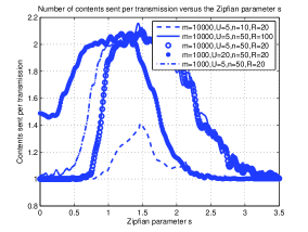
Figure 4: Average number of contents transmitted in each time slot when using index coding as a function of the Zipfian parameter $s$ using a suboptimal search.

Figure 5 compares the average number of requests satisfied per time slot by a helper between our proposed scheme and the baseline approach. For this simulation, a Zipfian content request distribution with parameter $s=2$ is assumed. The cell radius is 400 meters, D2D transmission range is assumed to be 100 meters and 1000 UTs are considered in this figure similar to the simulations in [14] and Figure 1. Notice that with the baseline approach at least 27 helpers are required to cover the entire network and 24, 20, 14 and 10 helpers can cover 97%, 93%, 78% and 62% of the network, respectively. Using multihop D2D communications with a maximum of three hops, 4 helpers can cover the entire network while 3 helpers can cover 95% of the network nodes. We have shown that even with our very simple heuristic algorithm, multihop D2D can significantly improve the helper utilization ratio. Note that in baseline approach, each helper can at most transmit one content per transmission, however, our approach can satisfy more than one request per transmission by taking advantage of the side information that is stored in nodes’ caches. As the number of requests per user increases, there are more possibilities of creation of cliques of large size which results in increasing the efficiency of helper nodes. The simulation is carried for content request probability of up to 0.3 since realistically, no more than one third of nodes at any given time, request contents in the network.

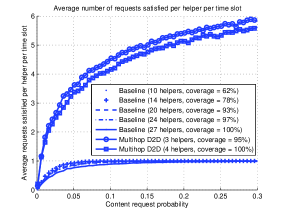
Figure 5: Comparing our proposed and baseline solution on average number of requests satisfied per time slot per helper versus the content request probability.

VII Conclusion

An efficient order optimal content delivery approach is proposed for future wireless cellular systems. We take advantage of femtocaches [14] and multihop communication using index coding. We proved that using index coding is very efficient technique by taking advantage of side information stored in UTs. Further, it was shown that under Zipfian content distribution, linear index coding could be order optimal. A heuristic graph coloring algorithm is proposed that achieves order optimal capacity bounds. Our simulation result demonstrates the gains that can be achieved with this approach.

Our proposed scheme improves the efficiency of femtocaches by taking advantage of multihop communications and index coding. One challenge of multihop communication is connectivity when nodes are moving fast. One solution is to divide the contents into equal smaller chunks and treat each chuck as a content. Another challenge is the additional delay imposed by using multihop communications. However, it is not readily clear that baseline approach provides lower delays. The reason is the fact that by using multihop communication, larger portion of the cell can be covered when the same number of femtocaches are used in both approaches as shown in Figure 1. A more detailed comparison of mobility and delay in single hop and multihop communication is the subject of future study. Security, overhead, routing are other issues that should be investigated in future works.

Mohsen Karimzadeh Kiskani received his bachelors degree in mechanical engineering from Sharif University of Technology in 2008. He got his Masters degree in electrical engineering from Sharif University of Technology in 2010. He got a Masters degree in computer science from University of California Santa Cruz in 2016. He is currently a PhD candidate in electrical engineering department at University of California, Santa Cruz. His main areas of interest include wireless communications and information theory. He is also interested in the complexity study of Constraint Satisfaction Problems (CSP) in computer science.

Hamid Sadjadpour (S’94-M’95-SM’00) received his B.S. and M.S. degrees from Sharif University of Technology and Ph.D. degree from University of Southern California, respectively. After graduation, he joined AT&T as a member of technical staff and finally Principal member of technical staff until 2001. In fall 2001, he joined University of California, Santa Cruz (UCSC) where he is now a Professor. Dr. Sadjadpour has served as technical program committee member and chair in numerous conferences. He has published more than 170 publications and has awarded 17 patents. His research interests are in the general area of wireless communications and networks. He is the co-recipient of best paper awards at 2007 International Symposium on Performance Evaluation of Computer and Telecommunication Systems (SPECTS), 2008 Military Communications (MILCOM) conference, and 2010 European Wireless Conference.

References

- [1] http://spectrum.ieee.org/telecom/wireless/millimeter-waves-may-be-the-future-of-5g-phones.
- [2] Amendments in IEEE 802.11ad™ enable multi-gigabit data throughput and groundbreaking improvements in capacity. https://standards.ieee.org/news/2013/802.11ad.html, 2013. [Online; accessed 9-October-2015].
- [3] Ziv Bar-Yossef, Yitzhak Birk, TS Jayram, and Tomer Kol. Index coding with side information. Information Theory, IEEE Transactions on, 57(3):1479–1494, 2011.
- [4] Federico Boccardi, Robert W Heath, Aurelie Lozano, Thomas L Marzetta, and Petar Popovski. Five disruptive technology directions for 5G. Communications Magazine, IEEE, 52(2):74–80, 2014.
- [5] Béla Bollobás. The chromatic number of random graphs. Combinatorica, 8(1):49–55, 1988.
- [6] Lee Breslau, Pei Cao, Li Fan, Graham Phillips, and Scott Shenker. Web caching and Zipf-like distributions: Evidence and implications. In INFOCOM’99. Eighteenth Annual Joint Conference of the IEEE Computer and Communications Societies. Proceedings. IEEE, volume 1, pages 126–134, New York, NY, 1999. IEEE.
- [7] Vikram Chandrasekhar, Jeffrey G Andrews, and Alan Gatherer. Femtocell networks: a survey. Communications Magazine, IEEE, 46(9):59–67, 2008.
- [8] Mohammad Asad R Chaudhry, Zakia Asad, Alex Sprintson, and Michael Langberg. On the complementary index coding problem. In Proceedings of Information Theory (ISIT), IEEE International Symposium on, pages 244–248, Saint Petersburg, Russia, 2011. IEEE.
- [9] Mohammad Asad R Chaudhry and Alex Sprintson. Efficient algorithms for index coding. In INFOCOM Workshops, IEEE, pages 1–4, Phoenix, AZ, 2008. IEEE.
- [10] Michelle Effros, Salim El Rouayheb, and Michael Langberg. An equivalence between network coding and index coding. Information Theory, IEEE Transactions on, 61(5):2478–2487, 2015.
- [11] Salim El Rouayheb, Alex Sprintson, and Costas Georghiades. On the index coding problem and its relation to network coding and matroid theory. Information Theory, IEEE Transactions on, 56(7):3187–3195, 2010.
- [12] P Erdős and L Pósa. On the maximal number of disjoint circuits of a graph. Publ. Math. Debrecen, 9:3–12, 1962.
- [13] Michael R Garey and David S Johnson. Computers and intractability. W. H. Freeman, San Francisco, 2002.
- [14] Negin Golrezaei, Karthikeyan Shanmugam, Alexandros G Dimakis, Andreas F Molisch, and Giuseppe Caire. Femtocaching: Wireless video content delivery through distributed caching helpers. In INFOCOM, Proceedings IEEE, pages 1107–1115, Orlando, FL, 2012. IEEE.
- [15] Ishay Haviv and Michael Langberg. On linear index coding for random graphs. In Information Theory Proceedings (ISIT), IEEE International Symposium on, pages 2231–2235, Cambridge, MA, 2012. IEEE.
- [16] Mingyue Ji, Giuseppe Caire, and Andreas F Molisch. Fundamental limits of caching in wireless D2D networks. Information Theory, IEEE Transactions on, 62(2):849–869, 2016.
- [17] Donald E Knuth. Big omicron and big omega and big theta. ACM Sigact News, 8(2):18–24, 1976.
- [18] Michael Langberg and Alex Sprintson. On the hardness of approximating the network coding capacity. Information Theory, IEEE Transactions on, 57(2):1008–1014, 2011.
- [19] Derek Leong, Tracey Ho, and Rebecca Cathey. Optimal content delivery with network coding. In Information Sciences and Systems, CISS, 43rd Annual Conference on, pages 414–419, Baltimore, MD, 2009. IEEE.
- [20] Jaime Llorca, Antonia M Tulino, Ke Guan, and Daniel Kilper. Network-coded caching-aided multicast for efficient content delivery. In Communications (ICC), IEEE International Conference on, pages 3557–3562, Budapest, Hungary, 2013. IEEE.
- [21] Mohammad Ali Maddah-Ali and Urs Niesen. Fundamental limits of caching. Information Theory, IEEE Transactions on, 60(5):2856–2867, 2014.
- [22] Marie-Jose Montpetit, Cedric Westphal, and Dirk Trossen. Network coding meets information-centric networking: an architectural case for information dispersion through native network coding. In Proceedings of the 1st ACM workshop on Emerging Name-Oriented Mobile Networking Design-Architecture, Algorithms, and Applications, pages 31–36, Hilton Head, SC, 2012. ACM.
- [23] Michael J Neely, Arash Saber Tehrani, and Zhen Zhang. Dynamic index coding for wireless broadcast networks. Information Theory, IEEE Transactions on, 59(11):7525–7540, 2013.
- [24] Tuan Tran, Thinh Nguyen, Bella Bose, and Vinodh Gopal. A hybrid network coding technique for single-hop wireless networks. Selected Areas in Communications, IEEE Journal on, 27(5):685–698, 2009.
- [25] Qinghua Wu, Zhenyu Li, and Gaogang Xie. Codingcache: multipath-aware CCN cache with network coding. In Proceedings of the 3rd ACM SIGCOMM Workshop on Information-Centric Networking, pages 41–42, Hong Kong, 2013. ACM.