Exciton-driven quantum phase transitions in holography

Abstract

We study phase transitions driven by fermionic double-trace deformations in gauge-gravity duality. Both the strength of the double trace deformation and the infrared conformal dimension/self-energy scaling of the quasiparticle can be used to decrease the critical temperature to zero, leading to a line of quantum critical points. The self-energy scaling is controlled indirectly through an applied magnetic field and the quantum phase transition naturally involves the condensation of a fermion bilinear which models the spin density wave in an antiferromagnetic state. The nature of the quantum critical points depends on the parameters and we find either a Berezinskii-Kosterlitz-Thouless-type transition or one of two distinct second order transitions with non-mean field exponents. One of these is an anomalous branch where the order parameter of constituent non-Fermi liquid quasiparticles is enhanced by the magnetic field. Stabilization of ordered non-Fermi liquids by a strong magnetic field is observed in experiments with highly oriented pyrolytic graphite.

Keywords: AdS/CFT, strongly correlated electrons, quantum criticality, graphene

I Introduction

The anti-de Sitter/conformal Field Theory correspondence (AdS/CFT) or gauge/gravity duality is a new proving ground to describe strongly correlated systems, and its application to unresolved questions in condensed matter is an exciting new direction. It is especially compelling, as conventional methods, such as large-$N$ Ref.largeN and $(4-\epsilon)$-type Ref.epsilon expansions fail to describe quantum critical behavior in $2+1$-dimensional systems. The primary examples of such are the strange metal states in the high $T_{c}$ cuprates and heavy fermion systems. Both systems are characterized by anomalous behavior of transport and thermodynamic quantities. In heavy fermions, the Sommerfeld coefficient grows as the temperature is lowered, meaning that the effective mass of the electrons on the Fermi surface diverges or the Fermi energy of the electrons vanishes Ref.Schofield:2005 . In the strange metal phase of the high $T_{c}$ superconductors as well as in heavy fermions near a quantum phase transition, the resistivity is linear with temperature $\rho\sim T$. These anomalous behaviors are partly explained by the phenomenological marginal Fermi liquid model Ref.Varma:1989zz , and it is an early success of AdS/CFT that the marginal Fermi liquid can be seen to emerge as the low-energy dynamics of a consistent theory.

A particularly simple gravity description for strongly interacting finite density matter is the planar AdS-Reissner-Nordström (AdS-RN) black hole (BH), which is dual to a system at finite chemical potential. While the AdS-RN black hole is a natural starting point to study the universal aspects of finite charge density systems, the universality of a black hole makes it difficult to explain experiments that are keen on the nature of the charge carriers, such as transport properties (e. g. conductivity). In particular the dominance of Pauli blocking for observed physics, requires that at the minimum one needs to add free Dirac fermions to the AdS-RN background. A self-consistent treatment shows that this system is unstable to a quasi-Lifshitz geometry in the bulk Refs.Review:2010 ; Hartnoll:es ; czs2010 , that encodes for a deconfined Fermi liquid system Refs.Hartnoll:2010xj ; Sachdev:2010um ; Huijse:2011hp ; Sachdev:2011ze . Here we shall initiate the study of instabilities in the unstable metallic AdS-RN phase that are driven by Fermi bilinears.

The essential low-energy property of the metallic system dual to the AdS-RN black hole background is the emergence of Fermi surfaces Refs.Leiden:2009 ; MIT where the notion of a quasiparticle needs not be well defined, i.e. stable Ref.Faulkner:2009 . In Ref.Leiden:2010 , we used the magnetic field as an external probe to change the characteristics of the Fermi surface excitations and as a consequence the transport properties of the system. It strongly suggested that a quantum phase transition should occur when the underlying quasiparticle becomes (un)stable as a function of the magnetic field. The study in this article of the influence on stability of Fermi bilinears allows us to show that there is a phase transition between the two regimes and that for a specific set of parameters the critical temperature vanishes. Our work is therefore also a fermionic companion to Ref.Faulkner:2011 .

Continuing the connection of AdS models to actual observations, the results we find resemble other experimental findings in quantum-critical systems. At low temperatures and in high magnetic fields, the resistance of single-layer graphene at the Dirac point undergoes a thousandfold increase within a narrow interval of field strengths Ref.Novoselov-Geim:2007 . The abruptness of the increase suggests that a transition to a field-induced insulating, ordered state occurs at the critical field $h_{c}$ Ref.Checkelsky:2009 . In bilayer graphene, measurements taken at the filling factor $\nu=0$ point show that, similar to single layer graphene, the bilayer becomes insulating at strong magnetic field Ref.Cadden-Zimansky:2009 . In these systems, the divergent resistivity in strong magnetic fields was analyzed in terms of Kosterlitz-Thouless localization Ref.Checkelsky:2009 and the gap opening in the zeroth Landau level Ref.Novoselov:2009 . However, it remains a theoretical challenge to explain a highly unusual approach to the insulating state. Despite the steep divergence of resistivity, the profile of $\rho$ vs. $T$ at fixed $h$ saturates to a $T$-independent value at low temperatures, which is consistent with gapless charge-carrying excitations Ref.Checkelsky:2009 . Moreover, in highly oriented pyrolytic graphite in the magnetic field, the temperature of the metal-insulator phase transition $T_{c}(h)$ increases with increasing field strength, contrary to the $T_{c}(h)$ dependence in the classical low field limit Ref.Kopelevich:1999 . The anomalous $T_{c}(h)$ behavior has been successfully modeled within a dynamical gap picture Ref.Shovkovy:2d . The available data suggest that by tuning the magnetic field graphene approaches a quantum critical point, beyond which a new insulating phase develops with anomalous behavior $T_{c}(h)$. This picture is in agreement with expectations of quantum critical behavior, where e. g. in heavy fermion metal a new magnetically ordered state (antiferromagnet) emerges when tuned through the quantum critical point Ref.Schofield:2005 .

We shall see that the same qualitative physics emerges with our use of the the magnetic field as a knob to tune to the IR fixed point to gain some insight into the quantum critical behavior driven by fermion bilinears. In our gauge/gravity dual prescription, the unusual properties characteristic for quantum criticality can be understood as being controlled by the scaling dimension of the fermion operator in the emergent IR fixed point. The novel insight of AdS/CFT is that the low-energy behavior of a strongly coupled quantum critical system is governed by a nontrivial unstable fixed point which exhibits nonanalytic scaling behavior in the temporal direction only (the retarded Green’s function of the IR CFT is $G_{IR}^{R}\sim\omega^{2\nu}$) Ref.Faulkner:2009 . This fixed point manifests itself as a near-horizon region of the black hole with AdS₂ geometry which is (presumably) dual to a one-dimensional IR CFT. Building on the semilocal description of the quasiparticle characteristics by simple Dyson summation in a Fermi gas coupled to this 1+1-dimensional IR CFT Ref.FaulknerPol an appealing picture arises that quantum critical fermionic fluctuations in the IR CFT generate relevant order parameter perturbations of the Fermi liquid theory. Whether this is truly what is driving the physics is an open question. Regardless, quantum critical matter is universal in the sense that no information about the microscopic nature of the material enters. Qualitatively our study should apply to any bilinear instability in the strange metal phase of unconventional superconductors, heavy fermions as well as for a critical point in graphene. Universality makes applications of AdS/CFT to quantum critical phenomena justifiable and appealing.

The paper is organized as follows. In Sec. II, we review the AdS-RN black hole solution in AdS-Einstein-Maxwell gravity coupled to charged fermions and the dual interpretation as a quantum critical fermion system at finite density. In Sec. III we use the bilinear formalism put forward in Ref.czs2010 to explore an instability of a quantum system towards a quantum phase transition using the AdS dual description. We study a quantum phase transition to an insulating phase as a function of the magnetic field. For completeness we test the various phases by a spectral analysis in Sec. IV. We conclude by discussing a phase space in $(h,T)$ variables for a quantum critical matter at nonzero temperatures.

II Holographic fermions in the background of a dyonic black hole

The gravity dual to a $2+1$-dimensional CFT at finite density in the presence of a magnetic field starts with the Einstein-Maxwell action describing an asymptotically AdS₄ geometry

$$S_{g}=\frac{1}{2\kappa^{2}}\int d^{4}x\sqrt{-g}\left({\mathcal{R}}+6-\frac{1}{g_{F}^{2}}F_{MN}F^{MN}\right).$$ (1)

Here $A_{M}$ is the gauge field, $g_{F}^{2}$ is an effective dimensionless gauge coupling and the curvature radius of AdS₄ is set to unity. The equations of motion following from eq.(1) are solved by a dyonic AdS black hole, having both electric and magnetic charge

$$ds^{2}=\frac{1}{(1-z)^{2}}\left(-fdt^{2}+dx^{2}+dy^{2}+\frac{dz^{2}}{f}\right)$$ (2)

where the redshift factor $f$ and the vector field $A_{M}$ are given by

$$f = z\left(3-3z+z^{2}-(Q^{2}+H^{2})(1-z)^{3}\right),$$

$$A_{t} = \mu z,\;\;A_{y}=hx,\;\mathrm{with}~{}~{}\mu=g_{F}Q,\;\;h=g_{F}H.$$ (3)

The AdS boundary is reached for $z\rightarrow 1$, the black hole horizon is at $z\rightarrow 0$ and the electric and magnetic charge of the black hole $Q$ and $H$, encoding the chemical potential $\mu$ and magnetic field $h$ of the dual CFT, are scaled such that the black hole temperature equals

$$T=\frac{1}{4\pi}\left(3-(Q^{2}+H^{2})\right).$$ (4)

In these units, the extremal $T=0$ black hole corresponds to $Q^{2}+H^{2}=3$ and in this case the red shift factor develops a double zero at the horizon

$$f=3z^{2}(z-z_{*})(z-\bar{z}_{*}),\;\;z_{*}=(4+i\sqrt{2})/3.$$ (5)

To include the bulk fermions, we consider a spinor field $\psi$ in the AdS₄ of charge $q$ and mass $m$, which is dual to a fermionic operator ${\mathcal{O}}$ in the boundary CFT₃ of charge $q$ and dimension

$$\Delta_{\Psi}=\frac{3}{2}+m,$$ (6)

with $m\geq-\frac{1}{2}$ (in units of the AdS radius). The quadratic action for $\psi$ reads

$$S_{\psi}=\int d^{4}x\sqrt{-g}\left(\bar{\psi}\Gamma^{M}{\mathcal{D}}_{M}\psi-m\bar{\psi}\psi\right),$$ (7)

where $\bar{\psi}=\psi^{\dagger}i\Gamma^{\hat{t}}$, and

$${\mathcal{D}}_{M}=\partial_{M}+\frac{1}{4}\omega_{Mab}\Gamma^{ab}-iqA_{M},$$ (8)

where $\omega_{Mab}$ is the spin connection, and $\Gamma^{ab}=\frac{1}{2}[\Gamma^{a},\Gamma^{b}]$. Here, $M$ and $a,b$ denote the bulk space-time and tangent-space indices respectively, while $\mu,\nu$ are indices along the boundary directions, i. e. $M=(z,\mu)$. The Dirac equation in the dyonic AdS-black hole background becomes

$$\left(\Gamma^{\hat{z}}\sqrt{f}\partial_{z}+\Gamma^{\hat{z}}\frac{\sqrt{f}}{2(1-z)}(3+\frac{(1-z)f^{\prime}}{2f})-\Gamma^{\hat{t}}\frac{i(\omega+q\mu z)}{\sqrt{f}}-\frac{1}{(1-z)}m+\Gamma^{\hat{x}}\partial_{x}+\Gamma^{\hat{y}}i(k_{y}-qhx)\phantom{\sqrt{f}}\right)\psi=0$$ (9)

where $\psi$ is the Fourier transform in the $y$ directions and time. The $z$ and $x$ dependences can be separated as in Refs.Albash:2009wz ; Albash:2010yr ; Leiden:2010 . Define

$$P = \Gamma^{\hat{z}}\sqrt{f}\left(\partial_{z}+\frac{1}{2(1-z)}(3+\frac{(1-z)f^{\prime}}{2f})\right)-\Gamma^{\hat{t}}\frac{i(\omega+q\mu z)}{\sqrt{f}}-\frac{1}{(1-z)}m$$

$$Q = \Gamma^{\hat{x}}\partial_{x}+\Gamma^{\hat{y}}(ik_{y}-iqhx),$$ (10)

in terms of which the Dirac equation is $(P+Q)\psi=0$. In order to separate the variables, we can proceed by finding the matrix $U$ such that $UP\psi=-UQ\psi=\lambda\psi$. The idea is that, although $P$ and $Q$ do not commute, we can find $U$ so that $[UP,UQ]$ commute and can be diagonalized simultaneously Ref.Leiden:2010 . To this end, $U$ must satisfy the relations $\{U,\Gamma^{z}\}=0$, $\{U,\Gamma^{t}\}=0$, $[U,\Gamma^{x}]=0$, $[U,\Gamma^{y}]=0$. A clear solution is $U=[\Gamma^{z},\Gamma^{t}]$.

In a convenient gamma matrix basis (Minkowski signature) Ref.Faulkner:2009

$$\Gamma^{\hat{z}}=\left(\begin{array}[]{cc}-\sigma^{3}&0\\ 0&-\sigma^{3}\end{array}\right),\;\;\Gamma^{\hat{t}}=\left(\begin{array}[]{cc}i\sigma^{1}&0\\ 0&i\sigma^{1}\end{array}\right),\;\;\Gamma^{\hat{x}}=\left(\begin{array}[]{cc}-\sigma^{2}&0\\ 0&\sigma^{2}\end{array}\right),\;\;$$ (17)

$$\Gamma^{\hat{y}}=\left(\begin{array}[]{cc}0&\sigma^{2}\\ \sigma^{2}&0\end{array}\right),\;\;\Gamma^{\hat{5}}=\left(\begin{array}[]{cc}0&i\sigma^{2}\\ -i\sigma^{2}&0\end{array}\right)\equiv i\Gamma^{\hat{t}}\Gamma^{\hat{x}}\Gamma^{\hat{y}}\Gamma^{\hat{z}}.$$ (22)

the matrix $U$ equals

$$U=\left(\begin{array}[]{cc}-i\sigma^{2}&0\\ 0&-i\sigma^{2}\end{array}\right).$$ (25)

This choice of the basis allows one to obtain $k_{y}=0$ spectral functions in a simple way. In the absence of a magnetic field one can use rotational invariance to rotate to a frame where this is so. The gauge choice for the a magnetic field obviously breaks the isotropy, but the physical isotropy still ensures that the spectral functions simplify in this basis Ref.Leiden:2010 . The $x$-dependent part of the Dirac equation can be solved analytically in terms of Gaussian-damped Hermite polynomials $H_{n}(\sqrt{qh}(x+\frac{k_{y}}{qh}))$ with eigenvalues $\lambda_{n}=\sqrt{|qh|n}$ quantized in terms of the Landau index $n=0,1,\dots$ Refs.Albash:2009wz ; Albash:2010yr ; Leiden:2010 . The Dirac equation $(P-U^{-1}\lambda)\psi=0$, where $\lambda$ is a diagonal matrix in terms of $\lambda_{n}$ and whose square is proportional to the identity, then reduces to

$$\left((\partial_{z}+\frac{1}{2(1-z)}(3+\frac{(1-z)f^{\prime}}{2f}))\Gamma^{\hat{z}}-\frac{i(\omega+q\mu z)}{f}\Gamma^{\hat{t}}-\frac{m}{\sqrt{f}(1-z)}-U^{-1}\frac{\lambda_{n}}{\sqrt{f}}\right)\psi=0.$$ (26)

We introduce now the projectors $\Pi_{\alpha}$ that split the four-component bispinors into two two-component spinors $\Psi=(\psi_{1},\psi_{2})^{T}$ where the index $\alpha=1,2$ is the Dirac index of the boundary theory

$$\Pi_{\alpha}=\frac{1}{2}(1-(-1)^{\alpha}\Gamma^{\hat{z}}\Gamma^{\hat{t}}\frac{1}{|\lambda|}Q),\;\;\alpha=1,2,\;\;\Pi_{1}+\Pi_{2}=1.$$ (27)

The projectors commute with both $P$ and $Q$ (recall that $Q^{2}=\lambda^{2}1\!\!1$). At zero magnetic field projectors are given by $\Pi_{\alpha}=\frac{1}{2}(1-(-1)^{\alpha}\Gamma^{\hat{z}}\Gamma^{\hat{t}}\hat{k}_{i}\Gamma^{i})$ with unit vector $\hat{k}_{i}=\vec{k}/|\vec{k}|$. The projections $\psi_{\alpha}=\Pi_{\alpha}\psi$ with $\alpha=1,2$ therefore decouple from each other and one finds two independent copies of the two-component Dirac equation

$$\left(\partial_{z}+\frac{1}{2}(\frac{3}{1-z}+\frac{f^{\prime}}{2f})-\frac{i(\omega+\mu_{q}z)}{f}\sigma^{2}+\frac{m}{\sqrt{f}(1-z)}\sigma^{3}+\frac{\lambda_{n}}{\sqrt{f}}\sigma^{1}\right)\psi_{1;2}=0,$$ (28)

where the magnetic momentum $\lambda_{n}=\sqrt{2|qh|n}$ is Landau quantized with integer values $n=0,1,\dots$ and $\mu_{q}\equiv\mu q$. It is identical to the AdS-Dirac equation for an AdS-RN black hole with zero magnetic charge when the discrete eigenvalue $\lambda$ is identified with the (size of the) momentum $k$.

As we have shown in Ref.Leiden:2010 , solving eq.(28) is equivalent to solving the Dirac equation at zero magnetic field but with a rescaled chemical potential and fermion charge. At $T=0$ the mapping is given by Ref.Leiden:2010

$$(\mu_{q},h,q)\mapsto(\mu_{q,eff},\,h_{eff},\,q_{eff})=(\sqrt{3}q\sqrt{1-\frac{h^{2}}{3}},\,0,\,q\sqrt{1-\frac{h^{2}}{3}}),$$ (29)

which we will use further.

III Bilinear approach to particle-hole pairing

The objective of this paper is to use the magnetic field as a tool to probe our unstable quantum critical system dual to the dyonic AdS-RN geometry. We show that the instability is manifest in the appearance of ordering in the system: the magnetic field acts as a catalyzer for the particle-hole pairing. In particular, we will find an unusual behavior for the critical temperature of the normal to paired phase transition as the dialing of the magnetic field drives the system to a quantum crtitical point: for a critical magnetic field the critical temperature vanishes indicating a new emergent quantum critical point.

We will identify the bulk quantities in the bilinear approach which are dual to the sought-for quantities on the CFT side. We have given the setup of the bilinear formalism in Ref.czs2010 . Here, we will first give a concise review with the focus on the transport properties and the influence of magnetic fields, and then derive the bilinear equations relevant for computing the pairing gap.

III.1 Bulk propagators and currents

A controlled method for calculating the expectation value of some composite operator $J$ with the structure of a fermion bilinear ($J\sim\psi^{\dagger}\psi$) has been put forward in Ref.czs2010 and it is based on a relation between the bulk and the boundary propagator in the isotropic single-particle approximation. This allows us to identify the familiar quantities at the boundary by matching the resulting expression to known thermodynamic relations. The crucial object was identified in Ref.czs2010

$$J^{\mu}(E,p,z)=\int d\omega\int d^{2}k\bar{\psi}(\omega,k,z)\Gamma^{\mu}\psi(E-\omega,p-k,z)$$ (30)

and it is the spatial average of the $U(1)$ current four-vector in the bulk. The metric then assumes the form given in the first section by eq.(2) (so that the horizon is located at $z_{H}=0$ and the boundary is at $z_{0}\to 1$). Having defined the radial projection of the bulk Dirac equation in eq.(27) we can also define the radial projections of the current as

$$J^{\mu}_{\alpha}(E,p,z)=\int d\omega\int d^{2}k\bar{\psi}_{\alpha}(\omega,k,z)\gamma^{\mu}\psi_{\alpha}(E-\omega,p-k,z),$$ (31)

where $\alpha=1,2$ and $\gamma^{\mu}$ is a Pauli matrix acting in the boundary frame.

The boundary interpretation of this current is, however, subtler than the simple $U(1)$ conserved current which it is in the bulk Ref.czs2010 : it expresses the Migdal theorem, i.e. the density of quasiparticles in the vicinity of the Fermi surface. To see this, express the bulk spinors $\psi_{\alpha}(z)$ at an arbitrary value of $z$ through the bulk-to-boundary propagators $\mathcal{G}_{\alpha}(z,z^{\prime})$ and the boundary spinors $\psi_{\alpha}(z_{0})$ as

$$\psi_{\alpha}(z)=\mathcal{G}_{\alpha}(z_{H},z)\mathcal{G}_{\alpha}^{-1}(z_{H},z_{0})\psi_{\alpha}(z_{0}).$$ (32)

The meaning of the above expressions is clear: the spinors evolve from their horizon values toward the values in the bulk at some $z$, under the action of the bulk-to-boundary propagator $\mathcal{G}_{\alpha}(z,z^{\prime})$ acting upon them (normalized by its value at the boundary). To find the relation with the boundary Green’s function we need to know the asymptotics of the solutions of the Dirac equation (28) at the boundary, see eq.(158) in Appendix A

$$\psi_{1} \sim a_{1}(1-z)^{3/2-m}\psi_{0,+}^{in}+b_{1}(1-z)^{3/2+m}\psi_{0,-}^{in}$$

$$\psi_{2} \sim a_{2}(1-z)^{5/2-m}\psi_{0,+}^{in}+b_{2}(1-z)^{5/2+m}\psi_{0,-}^{in}.$$ (33)

On the other hand, the boundary retarded propagator is given by the dictionary entry Ref.Vegh:2009 , eq.(161), where $\gamma^{0}=i\sigma^{1}$.

The bulk-to-boundary Green’s function (in dimensionless units) can be constructed from the solutions to the Dirac equation Ref.Hartman:2010 as in eq.(156). Using eq.(158) and the expression for the Wronskian, we arrive at the following relation between the boundary asymptotics of the solutions $\psi^{in}$ and $\psi^{bdy}$

$$\psi^{in}_{\alpha}(z_{0})=\left(\frac{(1-z)^{-2m}}{G_{\alpha}}(-i\gamma^{0})+1\right)\psi^{bdy}_{\alpha}(z_{0}).$$ (34)

Taking into account the dictionary entry for the boundary propagator from eq.(161) and the representation eq.(32) for $\psi^{in}$ and $\psi^{bdy}$, the retarded propagator at the boundary is

$$G_{\alpha}=\lim_{z_{0}\to 1}(1-z_{0})^{-2m}\psi^{bdy}_{\alpha}(z_{0})(\psi^{in}_{\alpha}(z_{0}))^{-1}=\lim_{z_{0}\to 1}\mathcal{G}_{\alpha}(z_{H},z_{0})\gamma^{0}\mathcal{G}_{\alpha}(z_{H},z_{0})$$ (35)

with $z_{H}=0$. Using eq.(35) and the definition for the current in eq.(31) it can now be shown that the current $J^{\mu}_{1}\sim\int\bar{G}_{1}\gamma^{\mu}G_{1}$ for an on-shell solution becomes at the boundary Ref.czs2010

$$J^{\mu}_{1}(\omega=0,k=k_{F},z_{0}\to 1)=\frac{1+2m}{\mu}\int d\omega\gamma^{\mu}G_{1}(\omega,k_{F}).$$ (36)

It is well known Ref.Landau9 that the integral of the propagator is related to the charge density. In particular, for $\gamma^{\mu}=\gamma^{0}$ and for the horizon boundary conditions chosen so that $G=G_{F}$ (Feynman propagator), we obtain

$$J^{0}_{1}\equiv\int d\omega\psi_{1}^{\dagger}\psi_{1}=\frac{1+2m}{\mu}n_{F},$$ (37)

i.e. the bilinear $J^{0}$ directly expresses the charge density $n_{F}={\rm tr}\left(i\gamma^{0}G\right)|_{on-shell}\sim|b_{1}(k_{F})|^{2}$. Notice that to achieve this we need to set $\omega=k-k_{F}=0$, i.e. look at the location of the Fermi surface. By analogy, we can now see that the components $J^{1,2}$ correspond to current densities. In particular, the ratio of the spatial components $J^{i}_{1}/E^{j}$ in the external electric field $\mathbf{E}$ readily gives the expression for the conductivity tensor $\sigma_{ij}$. Finally, the formalism outlined above allows us to define an arbitrary bilinear $J^{A}=\int\bar{\psi}\hat{A}\psi$ and to compute its expectation value. By choosing the matrix $\hat{A}$ appropriately we are able to model particle-hole, particle-particle or any other current. Notice however that all bilinears $J^{A}$ are proportional on shell, as can be seen from eqs.(35-36), which hold also for any other matrix $\hat{A}$ sandwiched between the two bulk propagators. The proportionality is at fixed parameters ($\mu$, $T$, etc) so the dependences of the form $J^{A}(\mu)$ and $J^{A}(T)$ will be different for different choices of $\hat{A}$.

To introduce another crucial current, we will study the form of the action. (We will define our action to model the quantum phase transition and to define the pairing excitonic gap in section III.2.) We pick a gauge, eq.(3), so that the Maxwell field is $A_{\mu}=\left(\Phi(z),0,h(z)x,0,0\right)$, meaning that the non-zero components of $F^{\mu\nu}$ are $F^{z0}=\partial_{z}\Phi$, $F^{z2}=x\partial_{z}h$, $F^{12}=h$ and their antisymmetric pairs. The total action eqs.(1,7) is now

$$S = \int dzd^{3}x\sqrt{-g}\left(\frac{1}{2\kappa^{2}}\left({\mathcal{R}}+6-\frac{1}{4g_{F}^{2}}F_{MN}F^{MN}\right)+\bar{\psi}\Gamma^{M}{\mathcal{D}}_{M}\psi-m\bar{\psi}\psi\right)$$ (38)

$$+ \int d^{3}x\sqrt{-h}\left({\mathcal{R}}_{bnd}A_{\mu}n_{\nu}F^{\mu\nu}+\sum_{\alpha}\bar{\psi}_{\alpha}(-i\sigma^{3})\psi_{\alpha}\right),$$

where $\bar{\psi}_{\alpha}=i\psi_{\alpha}^{\dagger}\sigma^{1}$. The second integral is the boundary term added to regularize the bulk action, for which the fermion part vanishes on shell. Knowing the metric eq.(2) and the form of $A^{\mu}$, we find that the total action (free energy, from the dictionary) can be expressed as Ref.czs2010

$$\mathcal{F}=\mathcal{F}_{\mathrm{hor}}-\frac{1}{2}(\mu\rho+h\mathcal{M})+\frac{3}{2}K$$ (39)

where $\mathcal{F}_{\mathrm{hor}}$ is the free energy at the horizon, which does not depend on the physical quantities on the boundary as long as the metric is fixed Ref.czs2010 so we can disregard it here. In eq.(39), $\mu,\rho$ and $h,\mathcal{M}$ are the leading and subleading terms in the electric and magnetic field

$$\Phi(z\to z_{0})=\mu,\;\;\partial_{z}\Phi(z\to z_{0})=\rho,$$

$$h(z\to z_{0})=h,\;\;\partial_{z}h(z\to z_{0})=\mathcal{M},$$ (40)

and the fermionic contribution is proportional to

$$K=\int d\omega\int d^{2}k\sum_{\alpha}\bar{\psi}_{\alpha}(\omega,k,z)\psi_{\alpha}(E-\omega,p-k,z)$$ (41)

which brings us to the second crucial bilinear. Along the lines of the derivation eqs.(31-36), we see that the fermionic contribution to the boundary action eq.(38) is proportional to

$$K=2\sum_{\alpha}{\rm Re}G_{\alpha},$$ (42)

i. e. it is the real part of the boundary propagator. The bulk fermionic term does not contribute, being proportional to the equation of motion, while the boundary terms include the holographic factors of the form $(1-z_{0})^{n}$. In accordance with our earlier conclusion that the on-shell bilinears are all proportional, we can reexpress the free energy in eq.(39) as

$$\mathcal{F}=\mathcal{F}_{\mathrm{hor}}-\frac{1}{2}(\mu\rho+h\mathcal{M})+\frac{3}{4m+2}\mu J^{0}_{1}$$ (43)

where the chemical potential reappears in the prefactor and the fermionic term becomes of the form $\mu J^{0}_{1}$, confirming again that $J^{0}_{1}$ can be associated with the number density.

III.2 Pairing currents

Now we will put to work our bilinear approach in order to explicitly compute the particle-hole (excitonic) pairing operator. We add a scalar field which interacts with fermions by the Yukawa coupling as done in Ref.Faulkner_photoemission:2009 . Both scalar and fermion fields are dynamical. The matter action is given by

$$S_{\psi} = i\int dzd^{3}x\sqrt{-g}\left(\bar{\psi}\Gamma^{M}D_{M}^{\psi}\psi-m_{\psi}\bar{\psi}\psi-\lambda|\phi|^{2}\bar{\psi}\psi\right)$$

$$S_{G} = \int dzd^{3}x\sqrt{-g}\frac{1}{2}G_{int}\left(\phi\bar{\psi}\Gamma\psi+\phi^{\star}\bar{\psi}\bar{\Gamma}\psi\right)$$

$$S_{\phi} = -\int dzd^{3}x\sqrt{-g}\left(|D_{M}^{\phi}\phi|^{2}+V(|\phi|)\right)$$ (44)

where the covariant derivatives are $D_{M}^{\psi}=\nabla_{M}+\frac{1}{4}\omega_{Mab}\Gamma^{ab}-iq_{\psi}A_{M}$, $D_{M}^{\phi}=\nabla_{M}-iq_{\phi}A_{M}$, and $\bar{\psi}=\psi^{\dagger}i\Gamma^{t}$. The gamma-matrix structure of the Yukawa interaction is specified further. Matter action is supplemented by the gauge-gravity action

$$S_{A}=\frac{1}{2\kappa^{2}}\int dzd^{3}x\sqrt{-g}\left(R+\frac{6}{L^{2}}-\frac{1}{4g_{F}^{2}}F_{MN}F^{MN}\right).$$ (45)

we take the AdS radius $L=1$ and $g_{F}=1$. The gauge field components $A_{0}$ and $A_{2}$ are responsible for the chemical potential and magnetic field, respectively, in the boundary theory. As in Ref.Faulkner_photoemission:2009 , we assume $\lambda=0$ and $V(|\phi|)=m_{\phi}^{2}|\phi|^{2}$ and the scalar is real $\phi^{\star}=\phi$. For the particle-hole sector, the scalar field is neutral $q_{\phi}=0$.

The Yukawa coupling $G_{int}$ is allowed to be positive and negative. When the coupling is positive $G_{int}>0$, a repulsive interaction makes it harder to form the particle-hole condesate. Therefore it lowers the critical temperature and can be used as a knob to tune to a vanishing critical temperature $T_{c}=0$ at a critical value $G_{int}^{c}$ which defines a quantum critical point. When the coupling is negative $G_{int}<0$, an attractive interaction facilitates pairing and helps to form the condensate.

Both situations can be described when the interaction term is viewed as a dynamical mass of either sign due to the fact that it is in $\bar{\psi}\psi$ channel. For $G_{int}>0$, interaction $G_{int}\phi$ introduces a new massive pole: massless free fermion field aquires a mass which makes it harder to condense. For $G_{int}<0$, there is a tachyonic instability. The exponentially growing tachyonic mode is resolved by a condensate formation, a new stable ground state. It can be shown that we do not need a nonzero chemical potential to form a condensate in this case. A similar situation was considered in Ref.Faulkner:2011 for the superconducting instability where the spontaneous symmetry breaking of $U(1)$ was achieved by the boundary double-trace deformation. In our case for the electron-hole pairing, $Z_{2}$ symmetry is spontaneously broken by a neutral order parameter. Next we discuss the choice for the gamma-matrix structure $\Gamma$ of the Yukawa interaction eq.(44) and the corresponding pairing parameter $\Delta$

$$\Delta=G_{int}\langle\bar{\psi}\Gamma\psi\rangle.$$ (46)

Now we explain our choice of the pairing operator and give a rigorous justification for this choice.

In principle, any operator that creates a particle and a hole with the same quantum numbers could be taken to define $\Delta$. This translates into the requirements

$$\left[\Gamma,\Gamma^{i}\right]=0,\{\Gamma,\Gamma^{0}\}=0,\left[\Gamma,\hat{C}\right]=0.$$ (47)

(Anti) commutation with (time) space gamma matrices is required for the preservation of homogeneity and isotropy, and the last one is there to preserve the particle-hole symmetry. In the basis we have adopted, eq.(22), $\left(\Gamma^{t}\right)^{\star}=-\Gamma^{t}$ and $\Gamma^{z\star}=\Gamma^{z}$, and therefore the charge conjugation is represented as

$$\hat{C}:\;\psi\rightarrow\Gamma^{0}\Gamma^{3}\psi^{\star}.$$ (48)

We will also consider the parity of the order parameter. As defined in Ref.Stefano-Bolognesi , parity in the presence of the AdS boundary acts as $x^{1}\rightarrow-x^{1}$ with $x^{2},z$ unchanged, while the transformation of the spinor is given by

$$\hat{P}:\;\psi\rightarrow\Gamma^{1}\Gamma^{5}\psi.$$ (49)

We can now expand $\Gamma$ in the usual basis

$$\mathbb{B}=\{I,\Gamma^{\mu},\Gamma^{5},\Gamma^{5}\Gamma^{\mu},\left[\Gamma^{\mu},\Gamma^{\nu}\right]\}$$ (50)

where the indices in the commutators $[\Gamma^{\mu},\Gamma^{\nu}]$ run along the six different combinations, and check directly that the conditions eq.(47) can only be satisfied by the matrices $I$, $\Gamma^{5}\Gamma^{i}$ and $[\Gamma^{0},\Gamma^{z}]$. This gives three candidate bilinears

• For $\Gamma=I$ we get the bulk current $\bar{\psi}\psi=-(\psi_{1}^{\dagger}\sigma^{1}\psi_{1}+\psi_{2}^{\dagger}\sigma^{1}\psi_{2})$, i.e. the mass operator in the bulk. As noted in this section and in more detail in Ref.czs2010 , it can be identified as proportional to the bulk mass term. As such, it describes the free energy per particle, as can be seen from the expression for the free energy eq.(39). The equation of motion for $K=\langle\bar{\psi}\psi\rangle$ eq.(41) exclusively depends on the $U(1)$ current and thus cannot encapsulate the density of the neutral particle-hole pairs: indeed, we directly see that the right-hand side equals zero if the total charge current vanishes.

• For $\Gamma=i\Gamma^{y}\Gamma^{5}$, the bulk current is $\bar{\psi}i\Gamma^{y}\Gamma^{5}\psi=-(\psi_{1}^{\dagger}\sigma^{1}\psi_{1}-\psi_{2}^{\dagger}\sigma^{1}\psi_{2})$. The crucial difference with respect to the first case is the relative minus sign. It is due to this sign that the current couples to itself, i.e. it is a response to a nonzero parameter $G_{int}$, as we will see soon.

• For $\Gamma=\Gamma^{z}$, the resulting bulk current is $\bar{\psi}\Gamma^{3}\psi=-i(\psi_{1}^{\dagger}\sigma^{2}\psi_{1}+\psi_{2}^{\dagger}\sigma^{2}\psi_{2})$. It sources the radial gauge field $A_{z}$ which is believed to be equal to zero in all meaningful holographic setups, as the radial direction corresponds to the renormalization group (RG) scale. Thus, this operator is again not the response to the attractive pairing interaction.

We are therefore left with one possibility only: $\Gamma=i\Gamma^{2}\Gamma^{5}$ which is also consistent with the choice of our gauge at nonzero magnetic field. We will therefore work with the channel

$$\Gamma\equiv i\Gamma^{y}\Gamma^{5}=\left(\begin{array}[]{cc}1&0\\ 0&-1\end{array}\right).$$ (51)

As we have discussed earlier, the isotropy in the $x-y$ plane remains unbroken by the radial magnetic field, and hence the expectation value should in fact be ascribed to the current $I^{\mu}=i\bar{\psi}\Gamma^{\mu}\Gamma^{5}\psi$ with $\mu=1,2$. We show the equivalence of the $i\Gamma^{x}\Gamma^{5}$ and $i\Gamma^{y}\Gamma^{5}$ order parameters below. The choice of the $y$ channel is motivated by technical simplicity due to the form of the projection operator and the fermion basis we use, eq.(27): $\Pi_{\alpha}=\frac{1}{2}\left(1-(-1)^{\alpha}\Gamma^{3}\Gamma^{0}\Gamma^{1}\right)$ with $\alpha=1,2$, since $\Gamma^{3}\Gamma^{0}\Gamma^{1}=-i\Gamma^{2}\Gamma^{5}$ with $\Gamma^{5}=i\Gamma^{0}\Gamma^{1}\Gamma^{2}\Gamma^{3}$. Finally, we note that the structure of the currents defined in eqs.(30,31) depends on the basis choice and that the currents as such have no physical interpretation in the boundary theory: physical meaning can only be ascribed to the expectation values Ref.czs2010 . It is exactly the expectation values that encode for the condensation (order) on the field theory side Refs.czs2010 , Stefano-Bolognesi .

The AdS/CFT correspondence does not provide a straightforward way to match a double-trace condensate to a boundary operator, though only single-trace fields are easy to identify with the operators at the boundary. Indeed, in holographic superconductors a superconducting condensate is modeled by a charged scalar field $\langle\Phi\rangle$ (see e.g. Ref.Horowitz:2009 ). As in Ref.Stefano-Bolognesi , we argue by matching discrete symmetries on the gravity and field theory sides, that the expectation of the bulk current $\langle\bar{\psi}i\Gamma^{2}\Gamma^{5}\psi\rangle$ is gravity dual of the pairing particle-hole gap. Let us consider properties of the corresponding condensates with respect to discrete symmetries, parity and charge conjugation, in the AdS four-dimensional space. According to eq.(49), $\langle\bar{\psi}\psi\rangle$ and $\langle\bar{\psi}\Gamma^{3}\psi\rangle$ are scalars and parity even, while $\langle\bar{\psi}i\Gamma^{2}\Gamma^{5}\psi\rangle$ is a pseudoscalar and parity odd. As for the charge conjugation, we easily find that $\langle\bar{\psi}\psi\rangle$ and $\langle\bar{\psi}i\Gamma^{2}\Gamma^{5}\psi\rangle$ commute with $\hat{C}$, while $\langle\bar{\psi}\Gamma^{3}\psi\rangle$ anticommutes. Since the latter is the component of a vector current while the former two are (pseudo)scalars, we find that all operators preserve the particle number, as promised. The magnetic field $H$ is odd under both parity and charge conjugation, and therefore it is unaffected by $\hat{C}\hat{P}$. The condensate $\langle\bar{\psi}\psi\rangle$ is also unaffected by $\hat{C}\hat{P}$, however $\langle\bar{\psi}i\Gamma^{2}\Gamma^{5}\psi\rangle$ and $\langle\bar{\psi}\Gamma^{3}\psi\rangle$ spontaneously break the $\hat{C}\hat{P}$ symmetry.

In the three-dimensional boundary theory, gamma matrices can be deduced from the four-dimensional bulk gamma matrices; and the four component Dirac spinor $\psi$ is dual to a two-component spinor operator $\Psi$. As has been also found in Ref.Stefano-Bolognesi , the three-dimensional condensate $\bar{\Psi}\Psi$ is odd under parity and even under charge conjugation, and therefore it is odd under $\hat{C}\hat{P}$. We summarize the transformation properties of the four- and three-dimensional condensates together with the magnetic field

$$\begin{array}[]{|c|c|c|c|c|c|}\hline\cr&\langle\bar{\psi}\psi\rangle_{4d}&\langle\bar{\psi}\Gamma^{3}\psi\rangle_{4d}&\langle\bar{\psi}i\Gamma^{2}\Gamma^{5}\psi\rangle_{4d}&\langle\bar{\Psi}\Psi\rangle_{3d}&H\\ \hline\cr\hat{P}&+&+&-&-&-\\ \hat{C}&+&-&+&+&-\\ \hat{C}\hat{P}&+&-&-&-&+\\ \hline\cr\end{array}$$ (52)

which shows that the symmetry properties are matched between $\langle\bar{\psi}i\Gamma^{2}\Gamma^{5}\psi\rangle_{4d}$ and $\langle\bar{\Psi}\Psi\rangle_{3d}$ condensates: they spontaneously break the CP symmetry while the magnetic field leaves it intact. Therefore our AdS/CFT dictionary between the bulk and boundary quantities is $\psi\leftrightarrow\Psi$ and $\langle\bar{\psi}i\Gamma^{2}\Gamma^{5}\psi\rangle\leftrightarrow\langle\bar{\Psi}\Psi\rangle$, with the corresponding conformal dimensions of boundary operators given by eq.(104) and eq.(103).

The natural bulk extension is now the current

$$I=(-i)\int d\omega\int d^{2}k\bar{\psi}(\omega,k,z)\Gamma\psi(E-\omega,p-k,z)$$ (53)

and it is understood that in nonzero magnetic field the integration over $k$ degenerates into the sum over Landau levels (this holds for all currents in this section). We will soon show that a complete set of bulk equations of motion for the operator eq.(53) requires a set of currents that we label $J_{\pm}$, $I_{\pm}$ and $K_{\pm}$. In the representation eq.(22) we introduce the following bilinears of the fermion field

$$J_{\pm}(E,p,z) = (-i)\int d\omega\int d^{2}k\left(\bar{\psi}_{1}(\omega,k,z)\sigma^{1}\psi_{1}(E-\omega,p-k,z)\pm\bar{\psi}_{2}(\omega,k,z)\sigma^{1}\psi_{2}(E-\omega,p-k,z)\right)$$

$$\equiv J_{1}(E,p,z)\pm J_{2}(E,p,z),$$

$$I_{\pm}(E,p,z) = (-i)\int d\omega\int d^{2}k\left(\bar{\psi}_{1}(\omega,k,z)\psi_{1}(E-\omega,p-k,z)\pm\bar{\psi}_{2}(\omega,k,z)\psi_{2}(E-\omega,p-k,z)\right)$$

$$\equiv I_{1}(E,p,z)\pm I_{2}(E,p,z),$$

$$K_{\pm}(E,p,z) = -\int d\omega\int d^{2}k\left(\bar{\psi}_{1}(\omega,k,z)\sigma^{2}\psi_{1}(E-\omega,p-k,z)\pm\bar{\psi}_{2}(\omega,k,z)\sigma^{2}\psi_{2}(E-\omega,p-k,z)\right)$$ (54)

$$\equiv K_{1}(E,p,z)\pm K_{2}(E,p,z),$$

where the pairing parameter $\langle\bar{\psi}\Gamma\psi\rangle$ in eq.(53) is $I\equiv I_{-}$, the index $0$ for the zeroth component is omitted in $J_{\pm}$, and $\bar{\psi}_{\alpha}=i\psi^{\dagger}_{\alpha}\sigma^{1}$.

Let us now study the dynamics of the system. We need to know the evolution equations for the currents and the scalar field and to complement them with the Maxwell equations. We will show that the equations of motion for all currents generically have nonzero solutions. This suggests that, due to the coupling with the UV CFT, the pairing can occur spontaneously, without explicitly adding new terms to the action (there is no need to add an interaction for fermions in the bulk). Nevertheless, we will also analyze the situation with nonzero $G_{int}$ and show what new phenomena it brings as compared to UV CFT-only coupling (i.e. no bulk coupling).

Let us start from the equations of motion. The Dirac and Klein-Gordon equations are to be complemented with the Maxwell equation

$$\nabla^{M}F_{MN}=iq_{\phi}\left(\phantom{1\over 1}\phi^{\star}(\nabla_{N}-iq_{\phi}A_{N})\phi-\phi(\nabla_{N}+iq_{\phi}A_{n})\phi^{\star}\phantom{1\over 1}\right)-iq_{\psi}\bar{\psi}\Gamma_{N}\psi$$ (55)

which is reduced when the scalar is real, $\phi^{\star}=\phi$, to

$$\nabla^{M}F_{MN}=2q_{\phi}^{2}\phi^{2}A_{N}-iq_{\psi}\bar{\psi}\Gamma_{N}\psi$$ (56)

In the background of a dyonic black hole with the metric

$$ds^{2}=\frac{1}{(1-z)^{2}}\left(-fdt^{2}+\frac{dz^{2}}{f}+dx^{2}+dy^{2}\right)$$ (57)

the Maxwell equation for the component $A_{0}$ is

$$\partial_{z}^{2}A_{0}-\frac{2q_{\phi}^{2}\phi^{2}}{(1-z)^{2}f}A_{0}-\frac{iq_{\psi}J_{+}}{(1-z)^{2}f}=0$$ (58)

where we have used $\bar{\psi}\Gamma_{0}\psi\rightarrow-J_{+}$.

In our setup we ignore the backreaction to $A_{2}=Hx$, treating it as a fixed external field. The justification comes from the physics on the field theory side: we consider a stationary nonmagnetic system with zero current and magnetization density. In the bulk, this means that the currents sourced by — and backreacting to — the magnetic field arise as corrections of higher order that can be neglected to a good approximation. Inclusion of the second Maxwell equation for $A_{2}$ would likely only lead to a renormalization of the magnetic field $H\mapsto H+\delta H$ without quantitative changes of the physics.

The equations of motion for the matter fields read

$$e_{A}^{M}\Gamma^{M}\left(\tilde{D}_{M}^{\psi}-iq_{\psi}A_{M}\right)\psi-m_{\psi}\psi-iG_{int}\phi\Gamma\psi=0$$

$$-(\partial_{M}-iq_{\phi}A_{M})(\partial^{M}-iq_{\phi}A^{M})\phi+\frac{1}{2}\frac{\phi}{|\phi|}V^{\prime}(|\phi|)-\frac{1}{2}G_{int}\bar{\psi}\Gamma\psi=0$$ (60)

where we included the connection to the definition $\tilde{D}_{M}=\nabla_{M}+\frac{1}{4}\omega_{Mab}\Gamma^{ab}$. In the dyonic black hole background, the Dirac equation is

$$\left[(\partial_{z}+{\mathcal{A}})\Gamma^{z}-\frac{i(\omega+qA_{0})}{f}\Gamma^{t}-\frac{m}{\sqrt{f}(1-z)}\mp\frac{iG_{int}\phi}{\sqrt{f}(1-z)}-U^{-1}\frac{\lambda_{n}}{\sqrt{f}}\right]\psi=0$$ (61)

where $q_{\psi}\equiv q$, the scalar is neutral $q_{\phi}=0$, $m_{\psi}\equiv m$ and

$${\mathcal{A}}=\frac{1}{2}\left(\frac{3}{(1-z)}+\frac{f^{\prime}}{2f}\right),\;\;A_{0}=\mu z,\;\;\lambda_{n}=\sqrt{2qhn},\;\;U^{-1}=\left(\begin{array}[]{cc}i\sigma^{2}&0\\ 0&i\sigma^{2}\end{array}\right)$$ (64)

with $f^{\prime}\equiv\partial_{z}f$. In the limit $\omega=0$ it is written as follows

$$\left(\partial_{z}+{\mathcal{A}}-\frac{iqA_{0}}{f}\sigma^{2}+\frac{m}{\sqrt{f}(1-z)}\sigma^{3}\pm\frac{iG_{int}\phi}{\sqrt{f}(1-z)}\sigma^{3}+\frac{\lambda_{n}}{\sqrt{f}}\sigma^{1}\right)\psi_{1;2}=0$$ (65)

We write the bilinears in short as

$$I_{\pm} = \psi_{1}^{\dagger}\sigma^{1}\psi_{1}\pm\psi_{2}^{\dagger}\sigma^{1}\psi_{2},$$

$$J_{\pm} = \psi_{1}^{\dagger}\psi_{1}\pm\psi_{2}^{\dagger}\psi_{2},$$

$$K_{\pm} = \psi_{1}^{\dagger}\sigma^{3}\psi_{1}\pm\psi_{2}^{\dagger}\sigma^{3}\psi_{2},$$ (66)

with $\bar{\psi}_{1}\equiv\psi_{1}^{\dagger}i\sigma^{1}$. Therefore $I_{-}=(-i)\bar{\psi}\Gamma\psi$ because $\bar{\psi}=\psi^{\dagger}\Gamma^{t}$. We rewrite the Dirac equation for the bilinears

$$(\partial_{z}+2{\mathcal{A}})J_{\pm}+\frac{2m}{\sqrt{f}(1-z)}K_{\pm}+\frac{2\lambda_{n}}{\sqrt{f}}I_{\pm}+\frac{2iG_{int}}{\sqrt{f}(1-z)}\phi K_{\mp}=0,$$

$$(\partial_{z}+2{\mathcal{A}})I_{\pm}+\frac{2qA_{0}}{f}K_{\pm}+\frac{2\lambda_{n}}{\sqrt{f}}J_{\pm}=0,$$

$$(\partial_{z}+2{\mathcal{A}})K_{\pm}-\frac{2qA_{0}}{f}I_{\pm}+\frac{2m}{\sqrt{f}(1-z)}J_{\pm}+\frac{2iG_{int}}{\sqrt{f}(1-z)}\phi J_{\mp}=0.$$ (67)

The pairing parameter is obtained by averaging the current $I_{-}$

$$\Delta=iG_{int}\langle I_{-}\rangle.$$ (68)

This system should be accompanied by the equation of motion for the neutral scalar field. In the limit of $\omega=0$ and $k_{i}=0$ it is given by

$$-\frac{1}{\sqrt{-g}}\partial_{z}\left(\sqrt{-g}\frac{1}{g_{zz}}\partial_{z}\phi\right)+\frac{1}{2}V^{\prime}(|\phi|)-\frac{1}{2}G_{int}\bar{\psi}\Gamma\psi=0$$ (69)

where $g\equiv{\rm det}g_{MN}$. In the dyonic black hole background, the equation of motion for the scalar is

$$\partial^{2}_{z}\phi+{\mathcal{B}}\partial_{z}\phi-\frac{m_{\phi}^{2}}{f(1-z)^{2}}\phi+\frac{iG_{int}}{2f(1-z)^{2}}I_{-}=0$$ (70)

where

$${\mathcal{B}}=\frac{2}{(1-z)}+\frac{f^{\prime}}{f}$$ (71)

The system of equations eq.(67) and eq.(70) is solved, at the lowest Landau level, for the unknown $I_{\pm},J_{\pm},K_{\pm}$ and $\phi$. We do not consider the backreaction of the spinor and scalar fields to the gauge field, and therefore we omit the Maxwell equation eq.(58).

Since the magnetic field is encapsulated in the parameter mapping eq.(29), we may put $\lambda_{n}=0$ and use the rescaled fermion charge; furthermore, the terms proportional to off-shell (discrete) momentum cancel out due to symmetry reasons, as explained in Ref.czs2010 . Another key property of the magnetic systems is that, at high magnetic fields, the ratio $\mu_{eff}/T$ can approach zero at arbitrarily small temperatures (including $T\to 0$).

Next we set up boundary conditions at the IR and UV for the system of equations eq.(67). It is enough to establish the boundary conditions for the fermion components. At the horizon we choose the incoming wave into the black hole. However, as we consider static solutions $\omega=0$, it is enough to take a regular solution, not growing to infinity as we approach horizon. We write the Dirac equation at the horizon $z\sim 0$ for the upper component $\psi_{1}=(y_{1},y_{2})$,

$$\left(\partial_{z}+{\mathcal{A}}-\frac{i\mu qz}{f}\sigma^{2}+\frac{m+G_{int}\phi}{\sqrt{f}(1-z)}\sigma^{3}+\frac{\lambda_{n}}{\sqrt{f}}\sigma^{1}\right)\left(\begin{array}[]{c}y_{1}\\ y_{2}\end{array}\right)=0$$ (74)

$${\mathcal{A}}=\frac{1}{2}\left(\frac{3}{1-z}+\frac{f^{\prime}}{2f}\right)$$ (75)

where at $T=0$ the metric factor is $f=z(3-3z+z^{2}-3(1-z)^{3})$. Near the horizon it becomes

$$\left(\partial_{z}+\frac{1}{2z}-\frac{i\mu_{q}}{6z}\sigma^{2}+\frac{m+G\phi}{z\sqrt{6}}\sigma^{3}+\frac{\lambda_{n}}{z\sqrt{6}}\sigma^{1}\right)\left(\begin{array}[]{c}y_{1}\\ y_{2}\end{array}\right)=0.$$ (78)

Explicitly, the system is written as

$$\partial_{z}y_{1}+\frac{1}{z}\left(\frac{1}{2}+\frac{m+G_{int}\phi}{\sqrt{6}}\right)y_{1}+\frac{1}{z}\left(\frac{\lambda_{n}}{\sqrt{6}}-\frac{\mu_{q}}{6}\right)y_{2}=0$$

$$\partial_{z}y_{2}+\frac{1}{z}\left(\frac{1}{2}-\frac{m+G_{int}\phi}{\sqrt{6}}\right)y_{2}+\frac{1}{z}\left(\frac{\lambda_{n}}{\sqrt{6}}+\frac{\mu_{q}}{6}\right)y_{1}=0.$$ (79)

The solution reads

$$y_{1} = C_{1}z^{-\frac{1}{2}-\nu}+C_{2}z^{-\frac{1}{2}+\nu}$$

$$y_{2} = \frac{1}{\frac{\mu_{q}}{6}-\frac{\lambda_{n}}{\sqrt{6}}}\left(C_{1}(\frac{m+G_{int}\phi}{\sqrt{6}}-\nu)z^{-\frac{1}{2}-\nu}+C_{2}(\frac{m+G_{int}\phi}{\sqrt{6}}+\nu)z^{-\frac{1}{2}+\nu}\right)$$ (80)

where $C_{1},C_{2}$ are constants and

$$\nu=\frac{1}{6}\sqrt{6(m+G_{int}\phi)^{2}+6\lambda_{n}^{2}-\mu_{q}^{2}}$$ (81)

We choose the solution with the regular behavior $y\sim z^{-\frac{1}{2}+\nu}$. The solution for $z_{i}$ in the lower component $\psi_{2}=(z_{1},z_{2})$ where $\psi=(\psi_{1},\psi_{2})$ is obtained from $y_{i}$ by a substitute $G_{int}\rightarrow-G_{int}$. We have for the bilinear combinations

$$I_{\pm} = y_{1}^{\dagger}y_{2}+y_{2}^{\dagger}y_{1}\pm(y\rightarrow z)$$

$$J_{\pm} = y_{1}^{\dagger}y_{1}+y_{2}^{\dagger}y_{2}\pm(y\rightarrow z)$$

$$I_{\pm} = y_{1}^{\dagger}y_{1}-y_{2}^{\dagger}y_{2}\pm(y\rightarrow z),$$ (82)

where $\psi_{1}=(y_{1},y_{2})$ and $\psi_{2}=(z_{1},z_{2})$.

We impose two boundary conditions for eq.(70): at the horizon $\phi^{\prime}(z=0)=0$ and at the AdS boundary $\phi(z=1)=0$.

At the AdS boundary, the boundary conditions for the currents are known from Ref.czs2010 : one should extract the normalizable components of $J,I,K$ in order to read off the expectation values. However, a normalizable solution is defined in terms of an absence of a source for the fundamental Dirac field $\psi_{\alpha}$ rather than the composite fields such as $J_{\pm}$. The solution is to put the source of the Dirac field to zero and then to read off the desired normalizable solution for $J_{\pm}$ directly. Under the assumption that the electrostatic potential $A_{0}$ is regular, from eq.(33) the composite field densities behave near the AdS boundary $z_{0}=1$ as

$$\mathcal{J}_{1}=\psi_{1}^{\dagger}\psi_{1}\rightarrow a_{1}^{2}(1-z)^{3-2m}+b_{1}^{2}(1-z)^{3+2m},$$

$$\mathcal{I}_{1}=\psi_{1}^{\dagger}\sigma^{1}\psi_{1}\rightarrow a_{1}b_{1}(1-z)^{3},$$

$$\mathcal{K}_{1}=\psi_{1}^{\dagger}\sigma^{3}\psi_{1}\rightarrow a_{1}^{2}(1-z)^{3-2m}-b_{1}^{2}(1-z)^{3+2m},$$ (83)

and

$$\mathcal{J}_{2}=\psi_{2}^{\dagger}\psi_{2}\rightarrow a_{2}^{2}(1-z)^{5-2m}+b_{2}^{2}(1-z)^{5+2m},$$

$$\mathcal{I}_{2}=\psi_{2}^{\dagger}\sigma^{1}\psi_{2}\rightarrow a_{2}b_{2}(1-z)^{5},$$

$$\mathcal{K}_{2}=\psi_{2}^{\dagger}\sigma^{3}\psi_{2}\rightarrow a_{2}^{2}(1-z)^{5-2m}-b_{2}^{2}(1-z)^{5+2m}.$$ (84)

The currents we have defined in eq.(54) are the averaged densities, e.g. $J_{1}=\int d\omega d^{2}k\mathcal{J}_{1}$. A normalizable solution in $\mathcal{J}_{\pm}=\mathcal{J}_{1}\pm\mathcal{J}_{2}$ is thus defined by the vanishing of both the leading and the subleading term.

In what follows the AdS evolution equations eq.(67) and eq.(70) with appropriate boundary conditions are solved numerically with a shooting method from the horizon. Unlike the recent study in Ref.Stefano-Bolognesi where only in the presence of the four-Fermi bulk coupling $G_{int}$ one finds a nontrivial solution for the averaged current $\langle I_{-}\rangle$ with the IR boundary taken at $z=0$, we will generically have a nonzero expectation value even for $G_{int}=0$. In Ref.Stefano-Bolognesi , one needed to introduce an IR cutoff, such as the hard wall, positioned at a radial slice $z=z_{\star}$. In our setup, the choice of the boundary conditions in the UV guarantees that the condensate will form irrespectively of the IR geometry, as it specifically picks the quasinormal mode of the fermion.

We repeat the same calculations for the $x$-component order parameter

$$\tilde{\Gamma}\equiv i\Gamma^{x}\Gamma^{5}=\left(\begin{array}[]{cc}0&1\\ 1&0\end{array}\right).$$ (85)

The pairing current defined as

$$\tilde{I}=(-i)\int d\omega\int d^{2}k\bar{\psi}(\omega,k,z)\tilde{\Gamma}\psi(E-\omega,p-k,z)$$ (86)

requires us to introduce the following currents

$$\tilde{J}_{\pm}(E,p,z) = (-i)\int d\omega\int d^{2}k\left(\bar{\psi}_{1}(\omega,k,z)\sigma^{1}\psi_{2}(E-\omega,p-k,z)\pm\bar{\psi}_{2}(\omega,k,z)\sigma^{1}\psi_{1}(E-\omega,p-k,z)\right)$$

$$\equiv \tilde{J}_{1}(E,p,z)\pm\tilde{J}_{2}(E,p,z),$$

$$\tilde{I}_{\pm}(E,p,z) = (-i)\int d\omega\int d^{2}k\left(\bar{\psi}_{1}(\omega,k,z)\psi_{2}(E-\omega,p-k,z)\pm\bar{\psi}_{2}(\omega,k,z)\psi_{1}(E-\omega,p-k,z)\right)$$

$$\equiv \tilde{I}_{1}(E,p,z)\pm\tilde{I}_{2}(E,p,z),$$

$$\tilde{K}_{\pm}(E,p,z) = -\int d\omega\int d^{2}k\left(\bar{\psi}_{1}(\omega,k,z)\sigma^{2}\psi_{2}(E-\omega,p-k,z)\pm\bar{\psi}_{2}(\omega,k,z)\sigma^{2}\psi_{1}(E-\omega,p-k,z)\right)$$ (87)

$$\equiv \tilde{K}_{1}(E,p,z)\pm\tilde{K}_{2}(E,p,z),$$

A tilde is used to distinguish the two cases of pairings involving $x$ and $y$ components. Using the Dirac equation at $\omega=0$

$$\left(\partial_{z}+{\mathcal{A}}-\frac{iqA_{0}}{f}\sigma^{2}+\frac{m}{\sqrt{f}(1-z)}\sigma^{3}+\frac{\lambda_{n}}{\sqrt{f}}\sigma^{1}\right)\psi_{1;2}+\frac{iG_{int}\phi}{\sqrt{f}(1-z)}\sigma^{3}\psi_{2;1}=0$$ (88)

where the pairing parameter is obtained by averaging the current $\tilde{I}_{+}$

$$\tilde{\Delta}=iG_{int}\langle\tilde{I}_{+}\rangle$$ (89)

we get the following set of coupled equations for the bilinears defined in eq.(87)

$$(\partial_{z}+2{\mathcal{A}})\tilde{J}_{\pm}+\frac{2m}{\sqrt{f}(1-z)}\tilde{K}_{\pm}+\frac{2\lambda_{n}}{\sqrt{f}}\tilde{I}_{\pm}+\frac{2iG_{int}}{\sqrt{f}(1-z)}\phi K_{+}=0,$$

$$(\partial_{z}+2{\mathcal{A}})\tilde{I}_{\pm}+\frac{2q\Phi}{f}\tilde{K}_{\pm}+\frac{2\lambda_{n}}{\sqrt{f}}\tilde{J}_{\pm}=0,$$

$$(\partial_{z}+2{\mathcal{A}})\tilde{K}_{\pm}-\frac{2q\Phi}{f}\tilde{I}_{\pm}+\frac{2m}{\sqrt{f}(1-z)}\tilde{J}_{\pm}+\frac{2iG_{int}}{\sqrt{f}(1-z)}\phi J_{+}=0.$$ (90)

There are no minus components for the $G_{int}\phi$ term in the first and third equations of eq.(90), and these terms contain currents without tildes defined in eq.(54). The equation of motion for the scalar is

$$\partial^{2}_{z}\phi+{\mathcal{B}}\partial_{z}\phi-\frac{m_{\phi}^{2}}{f(1-z)^{2}}\phi+\frac{iG_{int}}{2f(1-z)^{2}}\tilde{I}_{+}=0.$$ (91)

The system of equations (67), (70) and (90), (91) differ only in the $G_{int}$ term: they are identical without it, though currents are defined differently. Therefore, provided there is no ”source” in the equations of motion, i.e. there is no Yukawa interaction $G_{int}=0$, the $x$ and $y$ components of gamma matrices produce the vacuum expectation values (VEVs)

$$\langle I_{\pm}\rangle=\langle\tilde{I}_{\pm}\rangle$$ (92)

and according to the definitions of the pairing parameters

$$\Delta\to\langle I_{-}\rangle,\;\;\;\tilde{\Delta}\to\langle I_{+}\rangle$$ (93)

where $I_{\pm}$ is found from eq.(67). However, the equations for the plus and minus components in eq.(67) are identical. In particular,

$$\langle I_{+}\rangle=\langle I_{-}\rangle$$ (94)

which proves that $x$-$y$ rotational symmetry is intact and

$$\Delta=\tilde{\Delta}.$$ (95)

Further we consider only the $y$ component for simplicity.

III.3 Quantum criticality in the electron-hole channel

III.3.1 Thermodynamic behavior

We will first use the bilinear formalism to inspect the thermodynamics, in particular the phase transition that happens at high magnetic fields and the behavior of the pair density after the phase transition has occurred. To detect the transition, we can simply plot the free energy eq.(39) at a fixed temperature as a function of the magnetic field. The action can be rewritten in terms of the gauge field and currents as

$$S=\int dzd^{3}x\left(\frac{1}{2}\Phi\partial_{zz}\Phi+\frac{1}{2}H^{2}-I_{-}\Delta\right)$$ (96)

and we need to include also the boundary term that fixes the boundary values of the gauge field

$$S_{bnd}=\int d^{3}x\sqrt{-h}A_{\mu}n_{\nu}F^{\mu\nu}=\int d^{3}x\Phi\partial_{z}\Phi$$ (97)

where $n_{\mu}=(0,0,0,1)$ is the unit normal to the AdS₄ boundary, and $h$ is the induced metric for which $\sqrt{-h}=z_{0}^{-3}$. Identifying $\Phi(z_{0})=\mu$ and $\partial_{z}\Phi(z_{0})=\rho$ and using the Maxwell equation (58), we arrive at the final expression

$$\mathcal{F}=\mathcal{F}_{bulk}+\mathcal{F}_{bnd}=\int d^{3}x\left(\frac{(1-z_{0})^{1+2m}}{2\sqrt{f}}J_{+}\Phi+\frac{1}{2}h^{2}-I_{-}\Delta\right)+\int d^{3}x\left(\frac{\mu}{2m+1}J^{0}_{1}(1-z_{0})^{1+2m}+\frac{1}{2}\mu\rho\right)$$ (98)

In particular, we see that $I_{-}$ is indeed the response to the bulk order parameter $\Delta$. When the coupling $G_{int}$ is set to zero, the $I_{-}$ term in the bulk part of eq.(98) will be absent. Let us first see what happens in that case. The free energy is then unaffected by the pairing, and we can only follow the dependence on the magnetic field Fig.(1). We see the nonanalyticity in the free energy at the point $h=h_{c}$. The underlying mechanism can be understood from the mapping eq.(29): it is the disappearance of the coherent quasiparticle due to the lowering of the effective chemical potential $\mu_{eff}$. The pairing arises as a byproduct of the interaction with the boundary CFT and does not influence the transition.

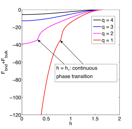
Figure 1: Total (bulk plus boundary) free energy of the system $\mathcal{F}(h)$ for increasing values of the charge $q$. An explicit pairing term $G_{int}=2$ has been chosen in order to suppress the stable Fermi surfaces and emphasize the phase transition at $h=h_{\star}$. Still, for higher $q$ values, the $\nu<1/2$ quasiparticles become subdominant compared to $\nu>1/2$ ones and the transition is lost. The bulk mass is $m=0.10$.

With the contact interaction, corresponding to electron-hole attraction in the infrared, we can further rewrite eq.(98) observing that generically

$$J_{1}(z,\omega)=\frac{1}{2}G_{R}(z,\omega)I_{-}(z,\omega),$$ (99)

which gives the following result for the fermionic free energy

$$\mathcal{F}_{f}=(1-z_{0})^{1+2m}J_{1}(z_{0},\omega=0)\left(\frac{3\mu}{4m+2}-2\Delta G_{R}^{-1}(\omega=0)\right).$$ (100)

The minus sign already makes it obvious that the derivative of the free energy can change sign, signifying a new critical point. To probe the transition point itself, however, we need to rewrite the relation eq.(99) for on-shell values. Then the denominator of $G_{R}$ vanishes, the current $J_{1}$ exactly captures the jump of the particle number on the Fermi surface Ref.czs2010 and eq.(37) becomes $J_{1}=3\mu/(2m+1)\times Z$, so we need to replace $G_{R}\mapsto Z$, which gives the equation for the critical point

$$\mathcal{F}_{f}=(1-z_{0})^{-2m}J_{1}(h)\left[\frac{3^{3/2}q}{4(\Delta_{\Psi}-1)}\sqrt{1-\frac{h^{2}}{3}}-\frac{2G_{int}I_{-}\left(h\right)}{Z(h)}\right].$$ (101)

We have also used $\Delta_{\Psi}=3/2+m$ in order to write the equation purely in terms of the boundary quantities, and emphasized that $Z$ and $J_{1}$ are also complicated functions of $h$, since $h$ determines the effective chemical potential. Notice that only $\mathcal{F}_{bnd}$ contributes to the fermionic term, while both $\mathcal{F}_{bulk}$ and $\mathcal{F}_{bnd}$ contribute to the gauge field term. For $G_{int}=0$, the second term vanishes and the free energy can only have a nonanalyticity when $J_{1}(h_{c})$ has it. It is a first order transition already identified in the magnetic case in Ref.Leiden:2010 and studied from a more general viewpoint in Ref.czs2010 : the magnetic field depletes the Landau levels of their quasiparticles and the Fermi surface vanishes. This first-order jump happens at some critical $\mu_{eff}$ and we will denote the corresponding value of the magnetic field by $h_{c}$. If, however, $G_{int}$ becomes finite, we can see that the first term decreases with $h$ while the second increases, since $Z(h)$ decreases. Thus, the overall free energy $\mathcal{F}=\mathcal{F}_{f}+\mathcal{F}_{gauge}$ will have a saddle point ($\mathcal{F}_{gauge}$ always decreases with $h$). We can now conclude that the following behavior with respect to $G_{int}$ can take place

• For $0\leq G_{int}<G_{int}^{0}$, the second term in eq.(101) is always negligible and the system only has the first-order transition at $h=h_{c}$.

• For $G_{int}^{0}<G_{int}<G_{int}^{1}$, the interplay of the first and the second term in eq.(101) gives rise to a local stationary point (but not an extremum) at some $h=h_{\star}$. This can potentially be a new critical point. In order to understand it better we will later perform a detailed analysis of the infrared behavior of the currents. It will turn out that it can be either a second order transition or an infinite order Berezinskii-Kosterlitz-Thouless (BKT)-type transition.

• For $G_{int}>G_{int}^{1}$, the Dirac hair cannot be formed and we have $J_{1}=0$ for any magnetic field, including zero. Since in this regime the pairing cannot occur even though $G_{int}$ is large, this means we are in fact outside the applicability of the mean field approach.

In Fig.(1) we show the second, arguably most interesting case. A second-order nonanalyticity in the free energy is obvious, as long as the stable quasiparticles with $\nu>1/2$ do not overpower the unstable quasiparticles that govern the transition at $h=h_{\star}$.

The conclusion we wish to emphasize is that order parameter physics is able to stabilize the non-Fermi liquids, while it is known Ref.Hartnoll:es ; czs2010 that in the absence of additional degrees of freedom a consistent backreaction treatment tends to leave only the stable, Fermi liquid surfaces. The physical nature of the point $h_{\star}$ will be the object of further analysis. The next section will reveal more on the actual pairing phenomenology, showing the new phase to be characterized by an anomalous, growing dependence $\Delta(h)$.

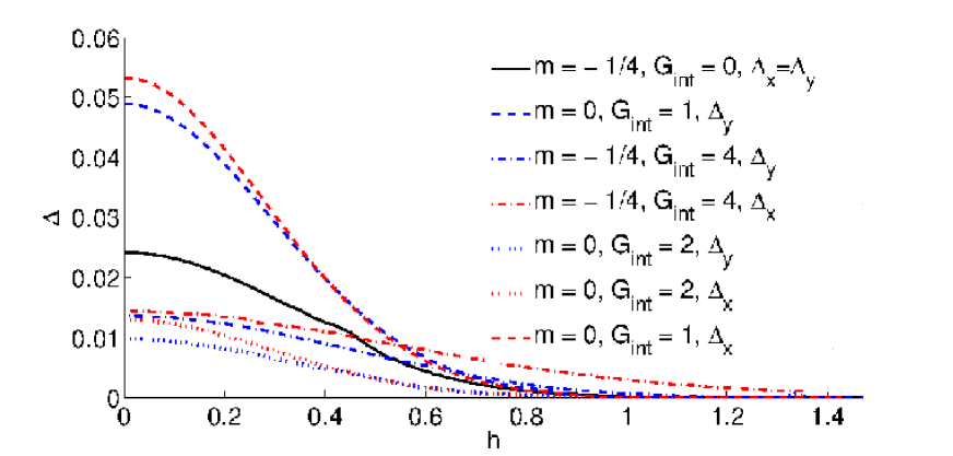
Figure 2: Dependence for the $x$ and $y$ components of the pairing order $\Delta_{x}(h)$ and $\Delta_{y}(h)$ for $G_{int}=0$ (coinciding solid line) and for $G_{int}=1,2,4$ (dashed, dotted and dashed-dotted lines). The coinciding solid line $\Delta_{x}=\Delta_{y}$ demonstrates the $x-y$ rotational invariance. For $G_{int}>0$, increasing the bare coupling decreases $\Delta$ (and lowers $T_{c}$) which provides a way to tune to the quantum critical point. Lowering the mass of the bulk fermion enhances pairing and increases $\Delta$ as seen for $m=0$ and $m=-1/4$.

III.3.2 Analysis of critical points

Having analyzed the thermodynamics and found the existence of critical points, we will now study the behavior of the order parameter $\Delta$ in the most interesting regime, for $G_{int}^{0}<G_{int}<G_{int}^{1}$, where the critical points are expected to appear.

In a nutshell, we will find that the region between $G_{int}^{0}$ and $G_{int}^{1}$ can be further subdivided into three regions, delimited by the values $G_{c}^{\star}$, $G_{c}^{\star\star}$ and $G_{c}$, characterized by one or two second order transitions or a BKT transition. We will also show that the pairing is favored for high effective chemical potentials when the density is high enough for the gravitational interaction to produce bound states. Finally, at small $h$ values the pairs vanish as $\Delta\propto\exp\left(\left(T_{c}-T\right)^{\beta}\right)$ with $0<\beta<1$ (presumably $\beta=1/2$) and finally reach zero density $\Delta=0$ for $T\leq T_{c}$, while for higher magnetic fields the trend is reversed and the order parameter starts growing with $h$.

In order to construct the phase diagram, we will first study $\Delta(h)$ at fixed temperature Fig.(3A). We see that for $m=-1/4$ (smooth curves) the gap vanishes following a function which is smoother than a power law. Indeed, it turns out that for $h<h_{c}$ we have the infinite order BKT scaling behavior

$$\Delta\sim\mu{\rm exp}\left(-\frac{C}{2\sqrt{q(h_{c}-h)}}\right).$$ (102)

The scaling eq.(102) will be proven in section IV. Similar behavior has been obtained in Ref.Iqbal:2010 where the scalar mass has been tuned to the quantum phase transition: $\Delta\sim\mu{\rm exp}\left(-\frac{C^{\prime}}{2\sqrt{m_{c}^{2}-m^{2}}}\right)$. Notice also that the value $h_{c}$ is very high, corresponding to the magnetic length of the order $\sqrt{h\mu_{eff}^{2}}\sim 10^{2}$ (we use $1/\mu_{eff}$ as the natural unit of length).

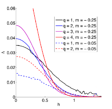
(A) (B)

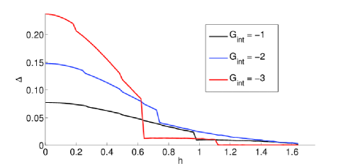
Figure 3: (A) Dependence $\Delta(h)$ (in dimensionless units) for $m=-1/4$ (smooth lines) and $m=-1/20$ and for increasing values of the fermion charge. At fixed fermion charge in the Fermi liquid regime ($\nu_{k_{F}}<1/2$), the magnetic field reduces the pair density, while small charges reduce the number of pairing particles, thus also reducing $\langle\Delta\rangle$. In the non-Fermi liquid regime ($\nu_{k_{F}}>1/2$) for $h>h_{c}$ we observe an anomalous, power-law growing behavior of the gap. (B) Dependence $\Delta(h)$ for $m=-1/4$ and the negative bulk coupling $G_{int}$. For increasing absolute values of the bulk coupling $G_{int}$ the pairing order $\Delta$ is enhanced. A new value $h_{\star}$ arises where the order parameter drops to zero due to competition between the channel $K_{1}$ and the quasiparticle density channel $I_{1}$. For large absolute value of $G_{int}$ eventually $h_{\star}=0$ and we are out of the mean field regime. The temperature is $T=5.6\times 10^{-4}$.

The above behavior is characteristic of the normal metal parent materials, i.e. $\nu_{k_{F}}>1/2$. At small values of $\nu_{k_{F}}$ (i. e. $\Delta_{\Psi}$ close to $3/2$ or small $\mu_{q}$), the anomalous growing dependence $\Delta(h)$ appears (found also in the previous section at strong enough magnetic fields) as shown by the dashed curves in Fig.(3A). The nature of the dependence $\Delta(h)$ is rooted in the unstable Fermi surfaces with $\nu_{k_{F}}\to 0$ and can be understood from the analysis of the bilinear equations in the AdS₂ region, which we postpone until the next section.

We study the relation $\Delta(h)$ at different values of the pairing coupling $G_{int}$. For $G_{int}>0$, $\Delta$ decreases as we increase $G_{int}$: repulsive interaction destructs the pairing, as given in Fig.(2). For $G_{int}<0$, $\Delta$ increases as absolute value of $G_{int}$ is increased: attractive interaction triggers and enhances the pairing, as given in Fig.(3B). Combining the two cases, when the sign of $G_{int}$ is taken into account, the dependence $\Delta$ versus $G_{int}$ is decaying. Lowering the mass of the bulk fermion enhances pairing as can be seen by comparing cases $m=0$ and $m=-1/4$ in Fig.(2). As shown in Fig.(2), pairing parameters with the $x$ and $y$ component are identical for $G_{int}=0$, which proves that the $x-y$ plane rotational symmetry is intact. As $G_{int}$ is switched on, it disrupts pairing in both channels in a slightly different way causing $\Delta_{x}$ and $\Delta_{y}$ to deviate from each other. An important novel feature distinguishing $G_{int}>0$ and $G_{int}<0$ is the appearance of the second anomalous branch for $G_{int}<0$ as seen in Fig.(3) where the magnetic field enhances pairing: the rising $\Delta(h)$ manifests magnetic catalysis (MC).

The motivation to consider $G_{int}>0$ was the ability to reduce the critical temperature to zero and to tune to the quantum critical point. On the other hand, adding $G_{int}<0$ increases the critical temperature; however we can tune to vanishing $T_{c}$ by adjusting other parameters such as the magnetic field. Figures (2) and(3B) can be used to extract the quantum critical point (QCP) $h=h_{c}$ when $\Delta=0$ (or $T_{c}=0$) at fixed $G_{int}$. Upon varying the coupling $G_{int}$, the QCP becomes the quantum critical line (QCL) $h_{c}(G_{c})$ or $G_{c}(h_{c})$. In Fig.(3B), for growing $G_{c}$, $h_{c}$ decreases in the normal branch and $h_{c}$ increases in the anomalous branch. In the normal branch, $h$ depletes the particles from the Fermi surface decreasing the pairing density. Therefore $h$ destroys condensate. In the anomalous branch though, $h$ enhances the condensation (magnetic catalysis).

The next step toward the phase diagram is the dependence of the critical temperature on the external magnetic field $T_{c}(h)$. A typical situation is given in Fig.(4A). We have captured both branches so we see the expected twofold behavior, with the decrease of $T_{c}$ up to $h=h_{c}$ and subsequent increase. A precise tuning of the mass toward zero is necessary to enter the quantum critical regime where $T_{c}(h_{c})=0$. For reference, we have also shown the cases $m=-0.10$ and $m=-0.05$, where the approach of the critical point is seen but $T_{c}(h_{c})$ is still a finite minimum.

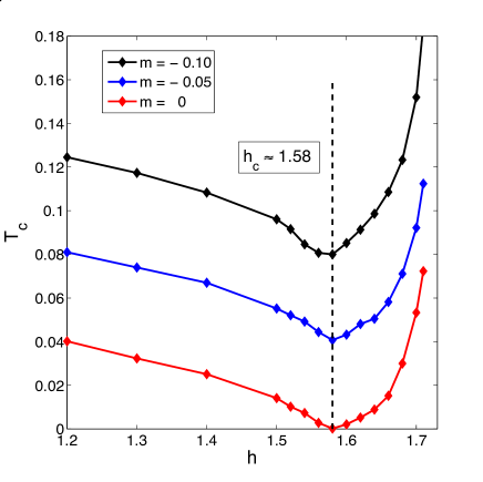
(A) (B)

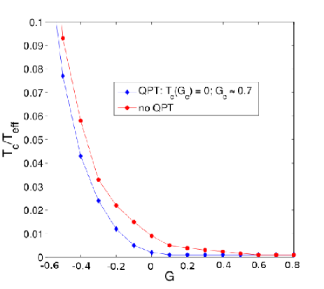
Figure 4: Critical temperature $T_{c}$ vs the magnetic field (A) and the coupling $G_{int}$ (B), for $q=1$. In (A), we again see the anomalous branch starting at $h_{c}\approx 1.58$, that signifies the exit from the Landau-Ginzburg regime and the mean field scaling into a new phase. Higher curves do not possess the QCP and arise when the system is always in the condensed phase. The coupling is $G=0.7$. In (B), we see $T_{c}$ vanish at the QCP $G_{c}\approx 1.1$, corresponding to the quantum phase transition (QPT) with a non-mean field exponent $T_{c}\sim|G_{c}-G|^{\beta}$, $\beta>1$. In the higher curve, $T_{c}$ remains nonzero for all $G_{int}$, with no QPT for this set of parameters. The bulk mass is $m=-0.10$.

Fig.(4B) shows the decreasing dependence of the critical temperature $T_{c}$ vs. the coupling strength $G_{int}$. For the blue curve $T_{c}$ vanishes at the QCP $G_{c}\approx 1.1$. It corresponds to the quantum phase transition (QPT) of the second order with a non-mean field exponent $T_{c}\sim|G_{c}-G|^{\beta}$, $\beta>1$. For the red curve, $T_{c}$ remains nonzero for all couplings $G_{int}$. It happens when the system is always in the condensed phase (an extreme RN AdS black hole is unstable) Ref.Faulkner:2010 . As seen from Fig.(4B), $G_{int}$ is a sensitive ”knob” to adjust the critical temperature $T_{c}$.

Finally, after studying the influence of the fermion charge $q$ and the bulk mass $m$ on the relation $T_{c}(h)$, we conclude with the Fig.(5), showing the critical temperature versus the magnetic field for different couplings $G_{int}$. We find four distinct regimes located in the interval $G^{0}<G<G^{1}$ (we omit the ”$int$” subscript in $G_{int}$ for now). The delimiting points are denoted by $G_{c}^{\star}$, $G_{c}^{\star\star}$ and $G_{c}$, with $G^{0}<G_{c}^{\star}<G_{c}^{\star\star}<G_{c}<G^{1}$.

• For $G<G_{c}^{\star}$ the critical temperature is nonzero, as demonstrated in Fig.(4B) and also by the red curve in Fig.(5). There is thus no QCP and the normal and anomalous regimes are separated by a crossover.

• For $G_{c}^{\star}<G<G_{c}^{\star\star}$, there are two second order phase transitions, one for the normal and one for the anomalous branch. This case is represented by the blue curve in Fig.(5), and can also be seen in Fig.(3A). The quantum phase transition corresponding to the anomalous branch scales with the non-mean field exponent $T_{c}\sim|h_{c}-h|^{\delta^{\prime}}$, $\delta^{\prime}>1$. The limiting case of $G=G_{c}^{\star}$ is given by the magenta curve, where the two critical points coincide.

• For $G_{c}^{\star\star}<G<G_{c}$, there is the second order phase transition with the non-mean field exponent $T_{c}\sim(h_{c}-h)^{\delta}$, $\delta<1$, which describes the normal branch. This is the dark violet curve in Fig.(5), similar to the regime in Fig.(3B).
  

• For $G>G_{c}$, there is an infinite order phase transition of the Berezinsky-Kosterliz-Touless (BKT) type with the characteristic exponential scaling $T_{c}\sim{\rm exp}\left(-\frac{C}{\sqrt{h_{c}-h}}\right)$. This is the black curve in the figure.

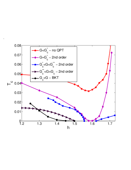
Figure 5: Critical temperature $T_{c}$ vs. the magnetic field $h$ for different couplings $G_{int}$. Depending on the coupling $G_{int}$, there are the BKT and second order phase transitions. At $T_{c}=0$, the QCP becomes QCL $(h_{c},G_{c})$ with a decreasing/increasing dependence on $h_{c}$ as $G_{c}$ is increased which corresponds to the normal/anomalous branch.

Finally, based on the data from Fig.(5) and some additional calculations, we can draw the phase diagram in terms of the magnetic field $h$ and the coupling $G_{int}$, given in Fig.(6). The QCL (solid line) separates the condensed (ordered) from uncondensed (disordered) phases. The position of the QCL is extracted from the phase transition curve of the critical temperature vs the magnetic field: the QCL where the critical temperature vanishes is given by the relation $G_{c}(h_{c})$. From the dependence $G_{c}(h)$, one can translate the scaling exponents $T_{c}$ vs. $G$ into $T_{c}$ vs. $h$: $T_{c}\sim|G_{c}-G|^{\beta}\to|G_{c}(h_{c})-G|^{\beta}\to|h_{c}-h|^{\delta}$.

In Fig.(6), increasing the coupling $G$ and the magnetic field $h$ destroy the pairing condensate except in the non-Fermi liquid regime. This twofold behavior manifests itself through a double-valued function $h_{c}(G_{c})$ in some parameter range. Indeed, the region with a condensed non-Fermi liquid is enhanced by the magnetic field, which is a consequence of the magnetic catalysis and the Callan-Rubakov effect discussed in the next section.

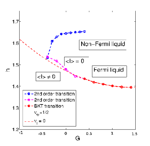
Figure 6: Phase diagram $h$ vs. $G$ for the condensed/normal (non-)Fermi liquids. $G$ and $h$ destroy the condensate except for the non-Fermi liquid. The ordered non-Fermi liquid is enhanced and stabilized by the strong magnetic field, which is also seen experimentally in pyrolytic graphite.

A deeper understanding of the phase diagram can be reached by considering the scaling dimensions of the condensate and the fermion field. With some foresight from the next subsection, we note that the IR conformal dimension of the operator which condenses $\delta_{\tilde{I}}=1/2+\nu_{\tilde{I}}$, where the bulk pairing current $\tilde{I}=\sqrt{\zeta}I$ is the gravity dual of the excitonic condensate, is given by eq.(115)

$$\nu_{\tilde{I}}=\sqrt{\frac{2}{3}}\sqrt{(m+\Delta)^{2}+2qh-\frac{\mu_{q}^{2}}{6}}.$$ (103)

On the other hand, the IR conformal dimension of the fermion operator $\delta_{\psi}=1/2+\nu_{\psi}$, where the bulk fermion field $\psi$ is dual to the boundary fermion $\Psi$, is given by

$$\nu_{\psi}=\frac{1}{6}\sqrt{m^{2}+k_{F}^{2}(h)-\frac{\mu_{q,eff}^{2}}{6}},\;\;\mu_{q,eff}=\sqrt{3}q\sqrt{1-h^{2}/3}.$$ (104)

Importantly, the ratio $\nu_{\tilde{I}}/\nu_{\psi}$ is first a decreasing and then an increasing function of the magnetic field $h$ (see left panel of Fig.(8) in Ref.Leiden:2010 for $\nu_{\psi}$). At the dashed line the IR dimension $\nu_{I}$ of the operator with gravity dual pairing current becomes imaginary, signaling the pairing instability. This is analogous to the instability of a scalar operator, when the Breitenlochner-Freedman (BF) bound in the AdS₂ is violated but the BF bound in the AdS₄ remains unbroken. The dash-dotted line corresponds to the locus of points in the phase diagram where $\nu_{\psi}=1/2$, separating the Fermi liquid from the non-Fermi liquid behavior as discussed in Ref.Faulkner:2009 . Since $\nu_{\psi}(h)$ is a monotonically decreasing function, coherent quasiparticles disappear at large magnetic field resulting in the non-Fermi liquid regime at $\nu_{\psi}\leq\frac{1}{2}$ (upper part of the phase diagram). Notably, there is a similarity between our phase diagram Fig.(6) and the phase diagram obtained for a scalar field Fig.(14) in Ref.Faulkner:2011 , which uses the double-trace deformation as the control parameter. This may provide an insight of a mechanism of suppression/enhancement of the ordered phase at small/large magnetic fields.

We can redraw our phase diagram in terms of the magnetic field $h$ vs. the chemical potential $\mu$, Fig.(7), to be able to compare our result with the literature Ref.Schmitt:2010 .

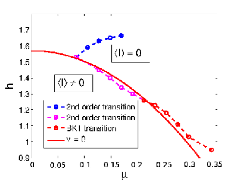
Figure 7: Phase diagram $h$ vs. $q$ for the condensed/normal (non-) Fermi liquids. Increasing the fermion charge at zero temperature is equivalent to increasing the chemical potential. It stabilizes the condensate in the anomalous regime and then destabilizes it in the normal branch. We can thus qualitatively relate $q$ to $G$, the coupling constant from the previous figure.

It is worth noting that our phase diagram exhibits the same main features as the analogous phase diagram obtained using the Sakai-Suggimoto model (Fig.(8) in Ref.Schmitt:2010 ). Primarily, it also has two regions of weak magnetic field where the condensate is destroyed by the magnetic field (”inverse” magnetic catalysis) and a regime of strong magnetic field which enhances the condensate (magnetic catalysis). Likewise, Fig.(5) shows the same structure as the analogous Fig.(9b) in Ref.Schmitt:2010 . Thus there are the two regimes with opposite dependence $\Delta(h)$. We will discuss the reasons for it in the next section.

III.3.3 Pairing, double-trace deformations and conformal field theory

We will conclude our study of the phase diagram by offering an alternative viewpoint of the observed critical phenomena. Dialing the pairing coupling to drive the system toward QPT can also be understood as dialing the double-trace deformation in the boundary theory Ref.Faulkner:2011 . For example, in the Gross-Neveu model with vector $SU(N_{f})$ symmetry, the four-fermion coupling operator is relevant at the UV fixed point. Hence, as a relevant deformation in UV, it can drive the RG flow of the system to a new IR fixed point with spontaneous symmetry breaking. In holography, the multitrace deformations which are introduced on the boundary and correspond to the multiparticle states in gravity are a powerful knob that can drive the theory either to a free CFT at the IR fixed point or to a CFT with the spontaneously broken symmetry. An RG flow of this kind has been considered in Ref.Gubser:2002 , where the relevant double-trace deformation at the UV fixed point drives the theory toward the asymptotically free IR fixed point. In the gravity dual theory, it corresponds to different boundary conditions imposed at the AdS₄ boundary (alternative/standard quantization), and the UV and IR CFTs are related by a Legendre transform Ref.Gubser:2002 .

As an illustration, consider a scalar theory in the bulk as in Ref.Iqbal:2010 . One can hope that this case captures the behavior of our system at least qualitatively as a bilinear fermion combination bosonizes into a scalar field. Fig.(8) shows schematically the two loop beta function for the double-trace coupling for decreasing magnetic field value. At strong magnetic fields, Fig.(8) top, the theory exhibits the usual RG flow from the strongly coupled UV fixed point (with a Landau pole at the QCP: $g_{c}\to\infty$) to a free fermion (a noninteracting theory at $g\to 0$) at the IR fixed point, with no expectation value for the scalar operator $O$. At the QCP i.e. $h=h_{c}$, Fig.(8) middle, the UV and IR fixed points merge and annihilate, leading to the BKT scaling Ref.Kaplan:2009

$$\Lambda_{IR}\sim\mu{\rm exp}\left(-\frac{C}{\sqrt{h_{c}-h}}\right)\sim\mu{\rm exp}\left(-\frac{C^{\prime}}{\sqrt{g-g_{c}}}\right),$$ (105)

which can be interpreted as a distance along the RG trajectory to get to the nontrivial IR fixed point with broken symmetry. In this case, the QPT is of infinite order and where the critical temperature $T_{c}$ and the order parameter $\langle O\rangle$ are governed by the exponential BKT scaling of eq.(105) as $T_{c}\sim\langle O\rangle\sim\Lambda_{IR}$. When the magnetic field $h$ is further decreased, Fig.(8) bottom, the theory becomes gapped leading to an apparent conformality loss Ref.Kaplan:2009 and the QPT is now of second order.

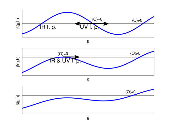
Figure 8: Two loop beta-function for the double trace coupling for decreasing magnetic field values. The disappearance of the original UV and IR fixed points at the critical magnetic field $h=h_{c}$ leads to conformality loss and the BKT scaling behavior, middle panel. At $h<h_{c}$, bottom panel, the system flows to a new IR fixed point with spontaneous symmetry breaking and nonzero condensate of a scalar field $\langle O\rangle\neq 0$.

In this paper we use the Yukawa coupling (or four-fermion coupling) in the bulk. However, the results we obtain are in line with the theory having a double-trace deformation on the boundary as described by Fig.(8): we have observed the rise of a new critical point. Fig.(3B) in particular conveys the message: at some $h_{\star}<h_{c}$ we observe a transition from the quasiparticle regime to an electron-hole condensate. Formally, it comes from the competition between the pairing channel and the particle-photon interaction, encoded by the bilinears $K_{1}$ and $I_{1}$. Physically, it corresponds to the competition between the Fermi surface ”order” and the pairing order. At $h=h_{c}$, it is the entrance into the non-Fermi liquid region ($\nu<1/2$) that drives the transition. At very high $G_{int}$ values, the pairing is again suppressed which we interpret as the consequence of the Fermi surface depletion. The number density near the Fermi momentum is given by the current $J_{0}$. In eq.(67), it is clear that the gauge field term, encoding for the chemical potential (and implicitly density), is competing with the term containing $\Delta(r)$, i.e. the term proportional to the coupling $G_{int}$. When the latter is dominant, the pairing is highly enhanced but only up to the point that all electrons are ”used up”, and their total number density is small. Notice also how $\Delta$ drastically increases at nonzero $G_{int}$, growing by about an order of magnitude.

III.4 AdS₂ analysis of the critical exponents

Most of our conclusions so far were driven by numerical results, with some qualitative analytical insight. A somewhat more detailed analytical understanding of the model can be gained by considering the far IR region, corresponding to the AdS₂ throat of the RN black hole.

We will follow the arguments of Ref.Iqbal:2010 , where it was shown by analyzing the AdS₂ region that a new IR scale $\Lambda_{IR}$ is generated which leads to the scaling behavior for the critical temperature $T_{c}$ and the condensate $\Delta$ vs a tuning parameter (the magnetic field in our case). The key point of this analysis is to show that an instability for a scalar field develops in a certain parameter range. In particular, for a neutral scalar field the mass should be lower than the AdS₂ BF bound, $m^{2}R^{2}<-\frac{3}{2}$ (where $R$ is the AdS₄ radius), which corresponds to a point where the IR conformal dimension becomes imaginary. For a charged scalar, the mass value can be slightly higher if the product of the charge and the chemical potential, $\mu_{q}$ is sufficiently large. We therefore consider a composite bosonic field, which can be constructed as a bilinear combination of $\psi$’s and in our case it is given by a bulk current.

Let us start by recalling that at $T=0$, the redshift factor develops a double zero near the horizon: $f\approx 6z^{2}$. Adopting the rescaled coordinates $\zeta,\tau$ instead of the dimensionless coordinates $z,t$:

$$\frac{1}{\frac{1}{z}-1}=\frac{\omega}{6\zeta},\;\;t=\frac{\tau}{\omega},$$ (106)

with $\omega\to 0$ and $\zeta,\tau$ finite, the metric eq.(2) becomes near the horizon

$$ds^{2}=\frac{1}{6\zeta^{2}}\left(-d\tau^{2}+d\zeta^{2}\right)+dx^{2}+dy^{2},$$ (107)

where the gauge field is

$$A_{\tau}=\frac{\mu}{6\zeta}.$$ (108)

In this metric, the currents defined in eq.(54) become

$$J(E,p,z) = (-i)\int d\omega\int d^{2}k\bar{\psi}(\omega,k,z)\sigma^{1}\psi(E-\omega,p-k,z),$$

$$I(E,p,z) = (-i)\int d\omega\int d^{2}k\bar{\psi}(\omega,k,z)\psi(E-\omega,p-k,z),$$

$$K(E,p,z) = -\int d\omega\int d^{2}k\bar{\psi}(\omega,k,z)\sigma^{2}\psi(E-\omega,p-k,z),$$ (109)

with $\bar{\psi}=i\psi^{\dagger}\sigma^{1}$. The Dirac equation at $\omega=k=0$ assumes the form

$$\left(\partial_{\zeta}-i\frac{\mu_{q}}{\sqrt{6}e_{\hat{\zeta}}}\sigma^{2}+\frac{(m+\Delta)}{e_{\hat{\zeta}}}\sigma^{3}+\frac{\lambda}{e_{\hat{\zeta}}}\sigma^{1},\right)\psi=0,$$ (110)

giving the following equations of motion for the currents

$$\partial_{\zeta}J+\frac{2(m+\Delta)}{e_{\hat{\zeta}}}K+\frac{2\lambda}{e_{\hat{\zeta}}}I=0$$ (111)

$$\partial_{\zeta}I+2\frac{\mu_{q}}{\sqrt{6}e_{\hat{\zeta}}}K+\frac{2\lambda}{e_{\hat{\zeta}}}J=0$$ (112)

$$\partial_{\zeta}K-2\frac{\mu_{q}}{\sqrt{6}e_{\hat{\zeta}}}I+\frac{2(m+\Delta)}{e_{\hat{\zeta}}}J=0$$ (113)

where $e_{\hat{\zeta}}=\sqrt{6}\zeta$, $\mu_{q}=\mu q$, $h_{q}=hq$, $\lambda=2|h_{q}|l$, $l=1,2,\dots$ and $\Delta=-\langle I\rangle$. Differentiating the second equation for $I$ with respect to $\zeta$ and eliminating the derivatives of $J$ and $K$ currents from the other two equations, we obtain the zero energy Schrödinger equation

$$\partial_{\zeta}^{2}\tilde{I}-\frac{\nu_{\tilde{I}}^{2}-1/4}{\zeta^{2}}\tilde{I}=0,$$ (114)

$$\nu_{\tilde{I}}=\sqrt{\frac{2\lambda^{2}}{3}-\frac{\mu_{q}^{2}}{9}},$$ (115)

where $\tilde{I}=I\sqrt{\zeta}$. We assume that condensation occurs for the lowest (first) Landau level ($l=1$) and it is caused by an instability when $\nu_{\tilde{I}}$ becomes imaginary. Therefore we can represent the conformal dimension as

$$\tilde{\nu}_{\tilde{I}}=\sqrt{\frac{4}{3}(h_{q}^{c}-h_{q})},\;\;h_{q}^{c}=\frac{\mu_{q}^{2}}{12}$$ (116)

where $\nu_{\tilde{I}}\equiv i\tilde{\nu}_{\tilde{I}}$, and $h_{q}^{c}$ is found from the condition $\nu_{\tilde{I}}=0$. Generalizing for $m\neq 0$ we get

$$\nu_{\tilde{I}}=\sqrt{\frac{2}{3}(\lambda^{2}+m^{2})-\frac{\mu_{q}^{2}}{9}},$$ (117)

$$h_{q}^{c}=-\frac{m^{2}}{2}+\frac{\mu_{q}^{2}}{12},$$ (118)

in dimensionless units.

Now consider the scaling behavior near the quantum critical point, $h\approx h_{c}$ or $G\approx G_{c}$ (solid red line in the phase diagram Fig.(6). As in Ref.Iqbal:2010 , imposing the Dirichlet boundary condition $\tilde{I}(\zeta=\zeta_{IR})=0$ gives an oscillatory solution of eq.(114)

$$I(\zeta)=\sin\left(\tilde{\nu}\log\frac{\zeta}{\zeta_{UV}}\right),$$ (119)

where $\zeta_{UV}$ is the location of the boundary of the AdS₂ throat. In order to satisfy the boundary condition we should have

$$\tilde{\nu}\log\frac{\zeta_{IR}}{\zeta_{UV}}=\pi.$$ (120)

According to the discussion in section IV of Ref.Iqbal:2010 , this means that a new IR scale is generated

$$\Lambda_{IR}\sim\frac{1}{\zeta_{h}}\sim\mu\rm{exp}\left(-\frac{\pi}{\tilde{\nu}}\right),$$ (121)

where $\mu$ is the UV scale, that leads to the infinite order BKT scaling behavior

$$T_{c}\sim\mu\rm{exp}\left(-\frac{C}{\sqrt{h_{q}^{c}-h_{q}}}\right),\;\;\Delta\sim\mu\rm{exp}\left(-\frac{C}{2\sqrt{h_{q}^{c}-h_{q}}}\right),$$ (122)

with $C=\frac{\pi}{\sqrt{4/3}}$ and $h_{q}^{c}$ given by eq.(118). The factor of $2$ in the exponent comes from the difference in operator dimensions in the intermediate conformal regime: the current $I$ scales as a dimension $1/2$ operator and the temperature scales with dimension $1$. Eq.(122) describes the behavior below the critical magnetic field $h<h_{c}$, which can be seen in Fig.(5). Since $h_{q}=hq$, increasing the charge $q$ would produce higher curves.

Choosing the mass $m$ as a tuning parameter, we obtain the infinite order BKT scaling behavior from the condition $\nu_{\tilde{I}}=0$ in eq.(118)

$$T_{c}\sim\mu\rm{exp}\left(-\frac{C^{\prime}}{\sqrt{m_{c}^{2}-m^{2}}}\right),\;\;\Delta\sim\mu\rm{exp}\left(-\frac{C^{\prime}}{2\sqrt{m_{c}^{2}-m^{2}}}\right),$$ (123)

with $C^{\prime}=\frac{\pi}{\sqrt{2/3}}$ and $m_{c}^{2}=-2h_{q}+\mu_{q}^{2}/6$. The scaling behavior from eqs.(122-123) describes the BKT regime found also for the condensation of a scalar field in Ref.Iqbal:2010 , with the condensed phase for $h<h_{c}$ (or at $m^{2}<m_{c}^{2}$) and the normal state with zero condensate at $h>h_{c}$ (or at $m^{2}>m_{c}^{2}$).

While the above analysis fits well into the results we have found for the normal branch, the anomalous branch, where at high $h>h_{c}$ the magnetic field catalyzes and enhances the condensate is still to be explained. The scaling behavior in this region is given by

$$T_{c}\sim\Delta\sim|h-h_{c}|^{\delta},$$ (124)

where $\delta>1$. In Figs.(3A,4A), a sharp increase with $h$ is found, which is in agreement with field theory calculations of magnetic catalysis Ref.Shovkovy:2d and experiments on graphite in strong magnetic fields Ref.Checkelsky:2009 . We leave the explanation of this regime within the AdS₂ analysis for further work.

For $m=0$, the equation of motion for $I$ can be reduced to a Schrödinger-like equation also in the general AdS₄ case. This is what we will do in the next subsection.

III.5 The $m=0$ formalism

As elucidated before in a slightly different context Ref.Faulkner:2009 , nonzero contributions to the current (corresponding to the quasiparticles at the boundary) are quantified by counting the bound states at zero energy for the formal wavefunction $I_{-}$ of the above equation. An important novel feature in our setup is that the momentum is quantized due to the magnetic field, and thus we cannot use the usual quasiclassical (WKB) formalism. Still, in the massless limit we will be able to gain some more insight by constructing an effective Schrödinger equation with a formal WKB momentum, that can be studied analytically.

Notice first that the RN geometry allows the spin connection term from eq.(8) to be absorbed in the definition of the currents as it is a total derivative Ref.Faulkner:2009

$$\mathcal{A}=\partial_{z}\left(-gg^{zz}\right)^{1/4}$$ (125)

Upon implementing eq.(125), the system of eqs.(67) for $m=0$ and in the static limit $\omega\to 0$ is simplified to

$$e_{\hat{z}}\partial_{z}J_{\pm}+2\Delta K_{\mp}+2e_{\hat{i}}\lambda I_{\pm}=0$$ (126a)

$$e_{\hat{z}}\partial_{z}I_{\pm}+2e_{\hat{t}}\Phi K_{\pm}+2\lambda e_{\hat{i}}J_{\pm}=0$$ (126b)

$$e_{\hat{z}}\partial_{z}K_{\pm}-2e_{\hat{t}}\Phi I_{\pm}+2\Delta J_{\mp}=0,$$ (126c)

where the vierbeine of the metric eq.(2) are $e_{\hat{z}}=(1-z)\sqrt{f}$, $e_{\hat{t}}=(1-z)/\sqrt{f}$, $e_{\hat{i}}=(1-z)$, and the scalar potential is rescaled as $q\Phi\to\Phi$ to absorb $q$. As before, the magnetic field is implemented by rescaling the chemical potential and the fermion charge as given by eq.(29), meaning that we can put $\lambda=0$. The expectation values are given by the minus component, with only three coupled equations for $J_{-},K_{-},I_{-}$ remaining to be solved. In order to understand the phenomenology of the bulk pair current, it is useful to eliminate $J_{-}$ from eq.(126). Rescaling $I_{-}$ as

$$I_{-}\mapsto\tilde{I}_{-}\equiv I_{-}\frac{e_{\hat{t}}\Phi}{e_{\hat{z}}}\equiv I_{-}\tilde{\Phi}$$ (127)

we first easily eliminate $J_{-}$ and differentiate eq.(126b) with respect to $z$. The derivative $\partial_{z}K_{-}$ can be expressed from eq.(126c) and $K_{-}$ from eq.(126b). In this way we arrive at the second order equation involving $I_{-}$ only and having the form of the Schrödinger equation for $\tilde{I}_{-}$

$$\partial_{zz}\tilde{I}_{-}-\left[\frac{2\partial_{z}\tilde{\Phi}}{\tilde{\Phi}}+4\tilde{\Phi}^{2}-\Delta\partial_{zz}\log\tilde{\Phi}\right]\tilde{I}_{-}=0.$$ (128)

Notice that the term containing the first derivative vanishes automatically due to the transform eq.(127).

We are interested in the behavior of the current in the limit $z\to z_{0}=1$. While the Schrödinger formulation might in some cases be more convenient also for computational reasons, the real benefit is that we can use a formal WKB scheme to arrive at surprisingly accurate solutions without solving the differential equation. Eq.(128) has the form $(\partial_{zz}-V_{eff}(z))\tilde{I}_{-}=0$, where the effective potential obeys the inverse square law near the boundary (we also use the relation eq.(89))

$$V_{eff}(z\to 1)=\delta^{2}(1-z)-\frac{8\Delta}{(1-z)^{2}}+\mu^{2}(1-z)^{2}+O(1)$$ (129)

where $\Delta\equiv\Delta(z\to z_{0})\approx\mathrm{const.}$: although, strictly speaking, one needs to compute $\Delta$ self-consistently given the value of $G_{int}$, for qualitative considerations we may assume a constant $\Delta$ proportional to $G_{int}$. The formal squared Dirac delta function is there to enforce the condition $J_{\pm}(z_{0})=I_{\pm}(z_{0})=K_{\pm}(z_{0})=0$. The typical appearance of the potential is given in Fig.(9). The development of the electron-hole condensate can be seen as the accumulation of bound states inside the potential well, analogously to the similar logic for electron states in Fermi and non-Fermi liquids, elucidated in Ref.Faulkner:2009 and applied in Ref.Leiden:2011 . We can easily visualize our findings on the transition points $h=h_{\star}$ and $h=h_{c}$ by looking at the potential Fig.(9). In the figures, we have left out the Dirac-delta squared spike at the boundary, as it is completely localized and only ensures that the currents reach zero at $z=1$, exerting no influence on the behavior at small but finite $1-z$ values. Importantly, the near-boundary gap opens with $\Delta>0$, supporting the electron-hole pair condensate near the boundary. The influence of the magnetic field through the relation $q\mapsto q\sqrt{1-H^{2}/(Q^{2}+H^{2})}$ is subtler: it makes the potential well both broader and shallower. The former generally facilitates the formation of bound states, while the latter acts against it. It is this competition that gives rise to the transition from the normal toward the anomalous region at $h=h_{c}$.

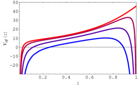
(A) (B)

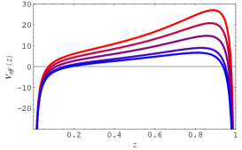
Figure 9: Effective potential for the current $\tilde{I}_{-}$ for $m=0,q=2,T=0.001\times 10^{-3}$ and $h=0$, $G_{int}=0,1/3,2/3,1$ (red to blue, A) and $G_{int}=0.2$, $h=0,0.50,1.00,1.50,1.71$ (red to blue, B). The pairing interaction opens the near-boundary gap (A), which gets wider but shallower as the magnetic field increases (B). The competition between the broadening and the shallowing effect gives rise to the transition between the normal and anomalous regime at $h=h_{c}$.

Within the WKB approximation, the solution to eq.(128) can be written as

$$\tilde{I}_{-}(z)=\frac{(1-z)^{2}}{\sqrt{V_{eff}(z)}}\left(\exp\left(-\sqrt{-V_{eff}(z)}\right)+\exp\left(\frac{3\pi}{4}i-\sqrt{V_{eff}(z)}\right)\right).$$ (130)

We have constructed the solution by equating the WKB expansion with the near-boundary expansion (eqs.(83,84)). Notice that the phase shift is $3\pi/4$ instead of the usual $\pi/4$, as the boundary itself provides an additional $\pi/2$ shift due to the condition $I_{-}(z_{0})\to 0$. The radial profile of the condensate is depicted in Fig.(10). It can be shown to have $\frac{1}{r^{3}}$ behavior at the UV boundary $r\to\infty$, and it diverges as $\frac{1}{r-1}$ at the horizon in the IR $r\to 1$. We obtain the same asymptotic behavior when $\Delta=0$ in eq.(129), but we impose the hard wall near the horizon in the IR, which brings us in agreement with the results of Ref.Stefano-Bolognesi . The UV behavior follows from the boundary condition on the fermion currents at the AdS boundary (putting the source term to zero) and the appearance of a fermion mass gap, to be discussed in more detail later.

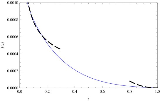
Figure 10: Radial profile of the excitonic condensate (solid line) from the numerical solution of the effective Schrödinger equation. The transformation law between radial coordinates is $r=\frac{1}{1-z}$. The fits (dashed lines) are the asymptotic behaviors $(1-z)^{3}\to\frac{1}{r^{3}}$ at $z\sim 1$ in the UV and $\frac{1}{z}\to\frac{1}{r-1}$ at $z\sim 0$ in the IR.

Another advantage of the Schrödinger approach is that solving the Schrödinger equation numerically is easier than solving the current equations. In Figs.(11-12) we give the dependences $\Delta(h)$ and $\Delta(q)$, produced by solving the equation (128). Qualitatively similar behavior is seen in both cases. The WKB approach makes it feasible to study also the dependence on the fermion charge $q$. Fig.(12) already shows that there is a critical value $q=q_{c}$ below which no pairing can occur at all. We conjecture that this value corresponds to $\nu<1/2$, i. e. only stable quasiparticles can pair up. While plausible, this is not easy to see from the relations $\Delta(h)$ and $\Delta(T)$ that we obtained in the $m\neq 0$ case.

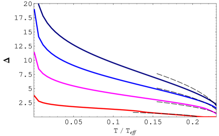
(A) (B)

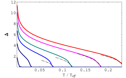
Figure 11: Order parameter of the pair density $\Delta$ vs the temperature (all in dimensionless units) (A) for $h=1$ and different values of the coupling strength $q=1,3,5,7$ (red, magenta, blue, black) and (B) for $q=3$ and different values of the magnetic field $h=0,0.8,1.2,1.4,1.6,1.7$ (red to black). Pairing is favored in the overdamped phase, with stable quasiparticles for $q\gg 1$ and $\nu\sim 1$, and suppressed at very high magnetic fields when the effective chemical potential is lowered and thus only a small number of electrons is available for pairing.

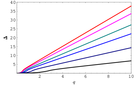
(A) (B)

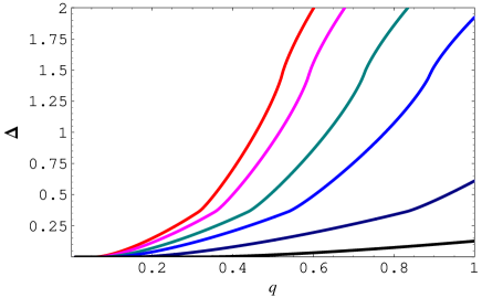
Figure 12: (A) Order parameter of the pair density $\Delta$ vs. the fermion charge $q$, for $T=5.6\times 10^{-4}$ and different values of the magnetic field $h=0,0.8,1.2,1.4,1.6,1.7$ (red to black). The critical value $q_{c}$ is shifted again due to the shifting of the effective potential. (B) Zoom-in near $q=0$ to better appreciate the transition.

IV Spectra and the pseudogap

In this section we will compute the spectra for the fermionic system with particle-hole pairs. We invoke again eqs.(28) to derive the equations of motion for the retarded propagator, which will directly give us the spectral function as $A(\omega,k)=\rm{Im}G_{R}$.

Following Ref.Faulkner:2009 , we can write a single nonlinear evolution equation for $G_{R}$. It will generically be a matrix equation, due to the additional, pairing channel. Of course, we can rewrite it as a system of four scalar equations for the four components of the bispinor. We adopt the basis given in eq.(22) and the metric given by eq.(2). Introducing the notation $\psi=(\psi_{1},\psi_{2})^{T}$ with $\psi_{\alpha}=(y_{\alpha},z_{\alpha})^{T}$ where $\alpha=1,2$, the resulting system reads

$$\left(\partial_{z}\mp m\sqrt{g_{zz}}\right)y_{1;2}=\mp i\sqrt{\frac{g_{zz}}{g_{ii}}}(\lambda-u)z_{2;1}-\Delta\sqrt{g_{zz}}y_{1;2}=0$$ (131a)

$$\left(\partial_{z}\mp m\sqrt{g_{zz}}\right)z_{1;2}=\pm i\sqrt{\frac{g_{zz}}{g_{ii}}}(\lambda+u)y_{2;1}+\Delta\sqrt{g_{zz}}z_{1;2}=0,$$ (131b)

with

$$u=\sqrt{\frac{g_{ii}}{-g_{tt}}}\left(\omega+q\Phi(z)\right).$$ (132)

Introducing $\xi_{\alpha}=iy_{\alpha}/z_{\alpha}$ as in Ref.Faulkner:2009 , where the boundary Green’s function is found from the asymptotics of the solution at the boundary (eqs.(33))

$$G_{\alpha}=\lim_{z\to 1}\left(\frac{1}{1-z}\right)^{2m}\xi_{\alpha}(z)=\lim_{\epsilon\to 0}\epsilon^{-2m}\xi_{\alpha}(1-z=\epsilon),$$ (133)

the equations of motion for $\xi_{\alpha}$ become

$$\partial_{z}\xi_{1;2}=-2m\sqrt{g_{zz}}\xi_{1;2}-\sqrt{\frac{g_{zz}}{g_{ii}}}(\lambda-u)+\sqrt{\frac{g_{zz}}{g_{ii}}}(\lambda+u)\xi_{1;2}^{2}\mp 2\Delta\sqrt{g_{zz}}\xi_{1;2}$$ (134)

The infalling boundary conditions at the horizon are imposed $\xi_{\alpha}=i$, while the amplitude of $y_{\alpha}$ remains free (it cancels out in the propagator $G_{R}$) and can be chosen to be of order unity for convenience in the numerical integration.

With no pairing channel, the morphology of the spectra is well known and has been analyzed in detail in Refs.Faulkner:2009 ; Leiden:2010 : near $k=k_{F}$, gapless quasiparticle excitations appear, belying a Fermi surface. Let us now repeat the AdS₂ analysis of Ref.Faulkner:2009 for the equations with pairing. We will use the $(\zeta,\tau)$ coordinates introduced in the eq.(106). The near-horizon equation of motion now assumes the following form

$$\zeta\partial_{\zeta}\psi=\left(i\sigma^{2}\frac{\mu_{q}}{6}-\sigma^{3}\frac{(m+s\Delta)}{\sqrt{6}}-\sigma^{1}\frac{k}{\sqrt{6}}\right)\psi,$$ (135)

where $s=\pm 1$, and in the presence of magnetic field the role of the momentum $k$ is taken over by Landau levels $\lambda=\sqrt{2|qh|l}$. Near the AdS₂ boundary ($\zeta\to 0$), the equation can be solved analytically at the leading order

$$\psi=A\left(\begin{matrix}\frac{m+s\Delta}{\sqrt{6}}+\nu\\ \frac{k}{\sqrt{6}}+\frac{\mu_{q}}{6}\end{matrix}\right)\zeta^{-\nu}+B\left(\begin{matrix}\frac{m+s\Delta}{\sqrt{6}}-\nu\\ \frac{k}{\sqrt{6}}+\frac{\mu_{q}}{6}\end{matrix}\right)\zeta^{\nu}$$ (136)

with

$$\nu=\frac{1}{6}\sqrt{\mu_{q}^{2}-6\left(\left(m+s\Delta\right)^{2}+k^{2}\right)},$$ (137)

and the self-energy scales as

$$\rm{Im}\Sigma\sim\omega^{2\nu}.$$ (138)

As usual, the Fermi surface is stable for $\nu^{2}>1/4$, unstable for $\nu^{2}<1/4$ and nonexistent for $\nu^{2}<0$.

In the bulk (and also as we move toward the boundary), the pairing term acts by shifting the mass as $m\mapsto m\pm\Delta$, meaning that the position of the quasiparticle pole is shifted, effectively modifying the $k_{F}$ value, which removes the spectral weight from the vicinity of $\omega=0$. It thus resembles a gap even though it is, strictly speaking, not a gap since the poles in $\psi_{1}$ and $\psi_{2}$ do not coincide (see also Ref.Faulkner_photoemission:2009 ). Nevertheless, we expect the size of the zero-weight region to be a useful benchmark for the degree to which the pairing eats up the (non-)Fermi liquid quasiparticles.

The typical appearance of the spectrum is given in Fig.(13), where we plot the spectra for $\Delta=0.2$ and for increasing magnetic field values. Increasing the magnetic field leads to destabilization of the quasiparticle (A,B), leading to a gap-like behavior, destabilization of the quasiparticle as seen from the asymmetry of the peak which loses its Fermi-liquid-like scaling. Eventually (C,D) the effective chemical potential is so low that we enter the ”almost conformal” regime. Fig.(14) shows the dependence on the pairing coupling: the peak at $\omega=0$ turns into a dip, a ”pseudogap” develops and we lose the quasiparticle.

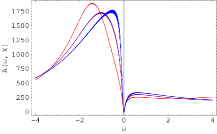
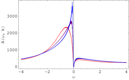
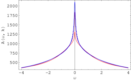
(A) (B) (C) (D)

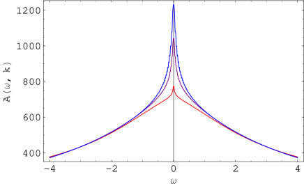
Figure 13: The spectral function $A(\omega,\lambda)$ for $\Delta=0.2$, $h=0.9,1.11,1.3,1.5$ (A,B,C,D) and three momentum values around $k_{F}^{\mathrm{eff}}$. At $h<h_{\star}$ (A,B) we see that $\nu^{2}<0$, corresponding to zero weight at $\omega\approx 0$, the phenomenon we have dubbed the pseudogap. For $h>h_{\star}$ (C,D) we enter the quasiconformal regime, with no Fermi surfaces left, the conformality being only slightly broken by nonzero $\Delta$.

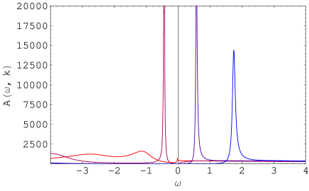
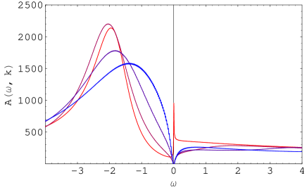
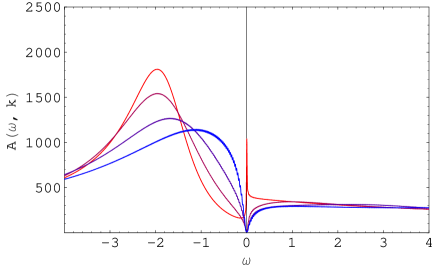
(A) (B) (C) (D)

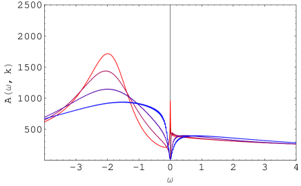
Figure 14: The spectral function $A(\omega,\lambda)$ for $h=0.2$, $\Delta=0.9,1.11,1.3,1.5$ (A,B,C,D) and four momentum values around $k_{F}^{\mathrm{eff}}$. At $\Delta<\Delta_{c}\approx 0.2$ (A), the quasiparticle peak survives; for higher $\Delta$ the influence of the exact value of the pairing term is negligible, and the spectrum always shows the pseudogap behavior.

V Discussion and conclusions

Before concluding the paper, we will discuss possible universal aspects of our findings, and show that the formation and enhancement of the particle-hole condensate in a strong magnetic field is a robust phenomenon seen in a number of distinct systems. We will limit ourselves to short remarks only, as more detailed comparisons with earlier work can be made by consulting the appropriate references.

We found the exciton instability using a Dirac hair or bilinear approach. A Dirac hair method uses bilinear combinations where a bilinear in a given channel develops an expectation value at the UV boundary provided a source is switched off. Dirac hair is equivalent to a Tamm-Dancoff approximation (TDA), planar diagrams of processes $2\rightarrow 2$ are included with no bulk fermion loops. In this sense, Dirac hair is a quantum mechanical treatment with one single classical wave function. It is quite remarkable to see that the condensate develops on a ”classical” level due to a nontrivial nature of the curved space-time with the help of the AdS/CFT dictionary, a phenomenon that was first obtained as a holographic superconductor Ref.Review:2010 .

We have associated the rising critical temperature vs magnetic field with the magnetic catalysis (MC), and the decreasing $T_{c}$ vs $h$ with the inverse MC (anomalous and normal branches in Fig.(5) for $G_{c}^{\star}<G<G_{c}^{\star\star}$, respectively). We adopted the terminology from Ref.Schmitt:2010 . It corresponds to a double-valued regime in the phase diagram Fig.(6). Similar behavior of increasing $T_{c}$ vs. the scalar mass $m$ has been observed in Ref.Iqbal:2010 under the action of a double-trace deformation, for the alternative quantization starting at the critical mass $m^{2}R^{2}\geq-\frac{27}{16}$. There it was associated with the formation of a new condensed phase corresponding to the high temperature regime. However, it was suggested that the high-T condensed phase is thermodynamically unstable Ref.Iqbal:2010 . Likewise, in Ref.Wang:2011 , exploring the phase diagram for a nonrelativistic conformal field theory, the authors found the high temperature condensate for $T\geq T_{H}$. The similarity of the dependences $\langle O\rangle(T)$ at different chemical potentials $\mu$ and $T_{c}(h)$ at different couplings $G$ to our Fig.(5) is obvious. In that work, the high temperature condensate was related to the high temperature instability predicted by Cremonesi et al. Ref.Cremonesi , and it was found to be thermodynamically disfavored over the trivial vacuum by direct calculation of the difference in the free energies Ref.Wang:2011 . However, the particle-hole condensate found at high magnetic fields in our case is crucially different from the unstable high temperature condensate in Refs.Iqbal:2010 ; Wang:2011 . Though naively both the magnetic field $h$ and the fermion mass $m$ destroy the condensate, increasing $m^{2}$ (or $h$) drives the bulk system to the UV(or the IR). Indeed, from the radial profile of the wave functions: at large $m$ the system resides near the UV boundary and at strong $h$ it resides near the RN black hole horizon in the IR, Fig.(5) in Ref.Leiden:2010 . Therefore, from holographic viewpoint large magnetic fields can lead to low-energy behavior and possible quantum critical phenomena, involving different ordering in the system. The main argument in favor of robustness and stability of our high-$h$ condensate is provided by the magnetic catalysis effect. In strong magnetic fields only the lowest Landau level contributes significantly to the ground state. Therefore, the dynamics is effectively dimensionally reduced as $d\to d-2$. In field theory this dimensional reduction leads to an increase in the density of states Ref.Shovkovy:1994 or in QCD to one-gluon exchange with a linear binding potential Ref.Chernodub:2010 , with both effects working towards pairing and enhancement of the condensate. In the AdS space, dimensional reduction leads to a Schwinger model showing an instability which is very similar to the Bardeen-Cooper-Schrieffer (BCS) pairing instability, where also the dynamics is effectively one-dimensional at the Fermi surface. The exact mapping between the magnetic catalysis at $h\neq 0$ and the BCS Cooper pairing at $\mu\neq 0$ has been established in Ref.Shovkovy:1994 .

We obtained a nontrivial radial profile and a boundary VEV for the bulk excitonic condensate $\langle\bar{\psi}\Gamma\psi\rangle$ at vanishing source, with the relation

$$\langle\bar{\psi}_{1}\psi_{1}\rangle=\frac{1}{2}\langle\bar{\psi}\psi\rangle-\frac{1}{2}\langle\bar{\psi}\Gamma\psi\rangle,\;\;\langle\bar{\psi}_{2}\psi_{2}\rangle=\frac{1}{2}\langle\bar{\psi}\psi\rangle+\frac{1}{2}\langle\bar{\psi}\Gamma\psi\rangle,$$ (139)

where $\Gamma=i\Gamma^{2}\Gamma^{5}$ and $\psi_{1,2}=\frac{1}{2}(1\mp\Gamma)\psi$ are the eigenvalues of the Dirac operator eq.(26) (the projectors $\Pi_{1,2}=\frac{1}{2}(1\mp\Gamma)$ are constructed out of gamma matrices which enter the Dirac operator only Ref.Faulkner:2009 ). We need to find the boundary condensate whose gravity dual is $\langle\bar{\psi}\Gamma\psi\rangle$ where the bulk Dirac field $\psi$ corresponds to a fermionic operator $\Psi$, $\psi\to\Psi$. The AdS/CFT correspondence does not provide a straightforward way to match a double-trace condensate to a boundary operator, though only gravity dual single-trace fields are easy to identify with the operators at the boundary. For example, in holographic superconductors a superconducting condensate is modeled by a charged scalar field $\langle\Phi\rangle$ (see e.g. Ref.Horowitz:2009 ). As in Ref.Stefano-Bolognesi , we find a boundary operator by matching discrete symmetries on the gravity and field theory sides and considering the asymptotic behavior of the gravity dual condensate at the boundary. As a result we associate a gravity dual excitonic order to some sort of a chiral condensate

$$\langle\bar{\psi}\Gamma\psi\rangle\leftrightarrow\bar{\Psi}\Psi$$ (140)

or some combination of condensates which break chiral symmetry. In Ref.Stefano-Bolognesi , this strategy provided the correspondence: $\langle\bar{\psi}\Gamma^{5}\psi\rangle\leftrightarrow\bar{\Psi}\Psi$. There an explicit use of the chiral basis $\psi_{L,R}=\frac{1}{2}(1\mp\Gamma^{5})\psi$ and the relation $\bar{\psi}_{L}\psi_{R}=\frac{1}{2}\langle\bar{\psi}\psi\rangle+\frac{1}{2}\langle\bar{\psi}\Gamma^{5}\psi\rangle$ made the correspondence evident. Specifically, by matching symmetries with respect to the discrete transformations eq.(52) we found that $\langle\bar{\psi}\Gamma\psi\rangle$ and $\langle\bar{\Psi}\Psi\rangle$ are pseudoscalars under parity and are unaffected by the charge conjugation, therefore they both spontaneously break the combination $\hat{C}\hat{P}$-symmetry. This finding is consistent with the existence of the parity odd mass in graphene associated with the excitonic order parameter in the $2+1$-dimensional effective field theory of graphene Refs.Shovkovy:2d ; Semenoff:2011 . Also the asymptotic behavior of the bulk condensate at the boundary, which was found numerically Fig.(10) to be $\langle\bar{\psi}\Gamma\psi\rangle\rightarrow C/r^{3}$ as $r\rightarrow\infty$, allows us to use a standard AdS/CFT dictionary to identify $C$ as the response or VEV of the boundary operator. The third power in the decay exponent indicates an extra mass scale. Indeed provided the response $\langle\Phi\rangle\sim 1/r^{3}$, the gauge-gravity duality gives a strong coupling form of the magnetic catalysis in $2+1$-dimensional Ref.Stefano-Bolognesi

$$\langle\bar{\Psi}\Psi\rangle\sim h\,M_{F},$$ (141)

with the magnetic field $h$ and mass gap $M_{F}$ Ref.Stefano-Bolognesi . It can be compared to the weak coupling field theory result $\langle\bar{\Psi}\Psi\rangle\sim h$ (we absorbed dimensional electric charge in the definition of magnetic field $h$, i.e. in $2+1$-dimensions the operator dimension is given by $[e]=\frac{1}{2}$ and $[h]=\frac{3}{2}$ with $[eh]=2$ and therefore we substitute $|e|h\rightarrow h$) Ref.Shovkovy:2d . Strong coupling realization follows from the anomalous fermion dimension $[\Psi]=\frac{3}{2}$ compared to the weak coupling conformal dimension $[\Psi]=1$ (free value dimension) in $2+1$-dimensional field theory. An extra fermion mass gap $M_{F}$ appears as a consequence of the dimensional four-fermion coupling $G_{int}=1/M_{F}$ in the bulk or introduction of the IR cutoff thought of as a hard wall at the radial slice $z_{\star}=1/M$. The authors of Ref.Stefano-Bolognesi have used the hard wall construction to obtain the strong coupling realization of the magnetic catalysis eq.(141). It is remarkable that the chiral condensate is proportional to the magnetic field even at strong coupling, that manifests the essence of the magnetic catalysis.

Another aspect of the chiral condensate is related to the Callan-Rubakov effect. As found in the field theory and also shown in the context of the gauge-gravity duality Ref.Stefano-Bolognesi2 , the chiral condensate can be spontaneously created in the field of a magnetic monopole. Due to the chiral anomaly $\partial j_{5}=F\tilde{F}$, the chiral symmetry is spontaneously broken and the chiral condensate $\langle\bar{\psi}\psi\rangle\sim{\rm e}^{i\Theta}/r^{3}$ is generated in the field of a monopole. In AdS, a construction involving a monopole wall (more precisely, a dyonic wall) and light fermions in the bulk produces an analog of the Callan-Rubakov effect resulting in the formation of the chiral-symmetry-breaking (CSB) condensate: $\langle\bar{\psi}\psi\rangle\neq 0$ Ref.Stefano-Bolognesi2 . The scaling behavior of the condensate is, however, different in our setup: as pointed out before, due to the lowest Landau level (LLL), the dimensional reduction $3d\to 1d$ takes place in the bulk. This reduces the equation of motion to an effective Schrödinger equation for the condensate, given by eq.(128) with the potential eq.(129). Solving the equation, we have found the IR behavior of the condensate near the horizon of the RN black hole ($1/r$) to be less divergent than the one near the monopole $\frac{1}{r^{3}}$ or the monopole wall $\frac{1}{(r-r_{w})^{3}}$ Ref.Stefano-Bolognesi2 .

It turns out that the AdS space with two boundaries: the UV boundary and the IR hard wall, plays an additional role in stabilizing the chiral condensate Refs.Stefano-Bolognesi ; Stefano-Bolognesi2 . It also provides an important hint for the interpretation of our current $\bar{\psi}\Gamma\psi$ in the boundary theory. In particular, for the lightest states to condense, we should take the LLL which only has one spin state available (instead of two states available for the higher LLs). This means that for a given charge, the spin direction is fixed. Therefore, fixing the direction of motion and the charge fixes also the helicity. Out of eight possibilities with a given charge, helicity and direction, only four are available for the LLL, as depicted at Fig.(15) (left). The charge $\pm$ denotes $e^{\pm}$, positive/negative helicity is denoted by R/L, and $S$ gives the spin orientation, lines with arrows show the momentum direction and $h$ stands for the magnetic field. The following bilinear combinations are possible when only LLL participate

• $\langle\bar{\psi}_{R\uparrow}\psi_{R\downarrow}\rangle$, $\langle\bar{\psi}_{L\uparrow}\psi_{L\downarrow}\rangle$ - (spin) scalar, charge neutral, momentum of the pair $\vec{P}=0$, chiral symmetry (CS) is not broken

• $\langle\bar{\psi}_{R\uparrow}\psi_{L\downarrow}\rangle$, $\langle\bar{\psi}_{L\uparrow}\psi_{R\downarrow}\rangle$ - (spin) scalar, charge neutral, momentum of the pair $\vec{P}\neq 0$, CS is broken

• $\langle\bar{\psi}_{R\uparrow}\bar{\psi}_{L\uparrow}\rangle$, $\langle\psi_{L\downarrow}\psi_{R\downarrow}\rangle$ - (spin) vector triplet, charged, momentum of the pair $\vec{P}=0$, CS is broken

We will not consider the first combination because it does not break the CS, and in our case CS is broken otherwise there would be no preferred scale for the current $I_{-}$. As for the third combination, it has been considered in the context of nonzero density QCD, where it describes the condensate of charged $\rho^{\pm}$ vector mesons Ref.Chernodub:2010 . It cannot be our order parameter either, since our current is a spin singlet. It is tempting to regard the doublet $\Gamma^{i}\Gamma^{5}$, $i=1,2$ as a vector, and we leave it for a future work.

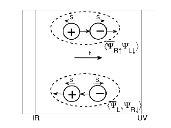
Figure 15: Formation of the chiral symmetry breaking excitonic condensate in the AdS space-time. Individual ”bouncing” events are shown schematically by the dashed lines. In an individual event, helicity flips while spin and charge are conserved.

We are thus left with the second combination. One can think of this order parameter as a spin-density wave, or magnetization which precesses around the direction of the magnetic field. The analog of the second combination has been considered within the Sakai-Sugimoto model as a holographic top-down approach to QCD Ref.Schmitt:2010 . The setting of Ref.Schmitt:2010 is very different from ours: it identifies the embedding coordinate of a probe D-brane with a scalar field dual to a single-trace fermion bilinear operator; the magnetic catalysis is modeled as bending of the probe brane under the influence of the magnetic field. There the anisotropic spatially modulated CSB condensate in the form of a single plane wave of Larkin-Ovchinnikov-Fulde-Ferrell (LOFF) state has been found. To have a condensate in the form of the second combination, we need to introduce the $SU(2)$ spin symmetry as in Ref.Iqbal:2010 . We should note the difference with our case where the construction of the condensate is done in the bulk and there is a special effort involved to identify the boundary operator. Provided the condensate of the second form is realized, the AdS boundary and the IR hard wall play a stabilizing role in its formation Ref.Stefano-Bolognesi2 . As the pair $\langle\bar{\psi}_{R\uparrow}\psi_{L\downarrow}\rangle$ ”bounces” from either of the boundaries it converts into the pair $\langle\bar{\psi}_{L\uparrow}\psi_{R\downarrow}\rangle$ conserving the total charge. This process can be decomposed into elementary ”bouncing” events

• $\bar{\psi}_{R\uparrow}\to\psi_{R\downarrow}$, $\psi_{L\downarrow}\to\bar{\psi}_{L\uparrow}$ - helicity is conserved, spin flips, mixing of charge occurs

• $\bar{\psi}_{R\uparrow}\to\psi_{L\uparrow}$, $\psi_{L\downarrow}\to\bar{\psi}_{R\downarrow}$ - helicity flips, spin and charge are unaffected

In the first case a particle deposits the charge at the boundary, which is picked up by the antiparticle, thus conserving the total charge of the particle-hole pair. The main difference between the two cases is either the ”bouncing” event involves spin flip or not, therefore either helicity is conserved or broken, respectively. By imposing the AdS boundary condition which breaks CS, helicity gets inverted by the boundary and CS breaking propagates from the boundary into the bulk. Then CS breaking occurs due to the boundary condition before the chiral condensate forms, which affects the propagation of the fields in the bulk in accordance with the second case stabilizing the condensate Ref.Stefano-Bolognesi .

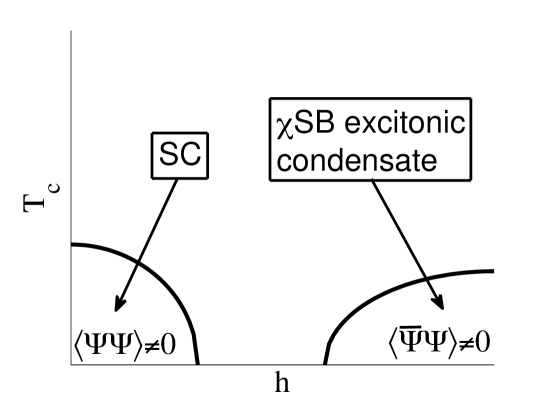
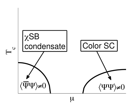
Figure 16: Analogy between the phase diagram of a condensed matter system at nonzero magnetic field and the QCD phase diagram at nonzero density. In strong magnetic fields, the excitonic condensate is mapped to the asymptotic regime of high chemical potential QCD with the color superconductor phase.

Next we discuss an analogy between the MC and the BCS Cooper pairing, and mapping between the Gross-Neveu model (or the Nambu-Jona-Lasinio (NJL)) in the presence of the magnetic field and the BCS model at nonzero chemical potential. The reason this mapping works is that effectively the dynamics in both cases is one dimensional: in the strong magnetic field the motion is constrained to Larmor orbits and includes only states from the lowest Landau level, while in a high density system only states at the Fermi surface contribute to the dynamics. We can draw the following analogy Ref.Schmitt-talk:2012

$$\begin{array}[]{|c|c|}\hline\cr{\rm MC}&{\rm BCS}\\ \hline\cr(3+1){\rm d}\to(1+1){\rm d}&(1+1){\rm d}\\ {\rm LLL\;\;and}\;\;\varepsilon=0\;\;{\rm surface}&{\rm Fermi\;\;surface}\;\;\varepsilon=\mu\\ \varepsilon=\sqrt{k_{z}^{2}+2|eh|n}&\varepsilon=k-k_{F},\;k=\sqrt{\vec{k}^{2}}\\ {\rm excitonic:}\;\;\Delta\sim G\langle\bar{\psi}\psi\rangle&{\rm SC:}\;\;\Delta\sim G\langle\psi\psi\rangle\\ \Delta\sim\sqrt{eh}\;{\rm exp}(-\frac{const}{G\nu_{0}})&\Delta\sim\mu\;{\rm exp}(-\frac{const}{G\nu_{F}})\\ \nu_{0}\;\;{\rm is\;\;DOS\;\;at}\;\;\varepsilon=0&\nu_{F}\;\;{\rm is\;\;DOS\;\;at}\;\;\varepsilon=\mu\\ h\;\;{\rm enhances},\;\;\mu\;\;{\rm destroys}\;\;\Delta&\mu\;\;{\rm enhances},\;\;h\;\;{\rm destroys}\;\;\Delta\\ \delta\Omega\sim h(\mu^{2}-\frac{\Delta^{2}}{2})&\delta\Omega\sim\mu^{2}(\delta\mu^{2}-\frac{\Delta^{2}}{2})\\ h\gg\mu,\Delta&\mu\gg\delta\mu,\Delta\\ {\rm it\;\;can\;\;have}\;\;\mu=0&{\rm it\;\;can\;\;have}\;\;h=0\\ T_{c}\;\;{\rm grows\;\;with}\;\;h\;\;({\rm MC})&T_{c}\;\;{\rm decreases\;\;with}\;\;h\\ T_{c}\;\;{\rm decreases\;\;with}\;\;\mu&T_{c}\;\;{\rm grows\;\;with}\;\;\mu\;\;({\rm SC})\\ \hline\cr\end{array}$$ (142)

where the acronym DOS stands for the density of states. Effectively one dimensional dynamics in both cases leads to similarities in formulas for the pairing gap $\Delta$ and the gain in thermodynamic potential $\delta\Omega$ as compared to the normal unpaired state. In the BCS, the density of states at the Fermi surface $\varepsilon=\mu$ defines the gap $\Delta$, and there is a an energy cost $\mu^{2}\delta\mu^{2}$ to bring two Fermi surfaces together to pair in case of nonzero mismatch $\delta\mu$ between them. In MC, the density of states at the $\varepsilon=0$ surface separating electrons and holes contributes to the gap, and a similar cost in energy $h\mu^{2}$ exists to involve both particles and holes to pair. The gain from the pairing is proportional to $\Delta^{2}$ in both cases, and is linear in $\mu^{2}$ for the BCS and in $h$ for the MC, manifesting the essence of both phenomena. These simple formulas for $\delta\Omega$ can be obtained when there is a hierarchy of scales: the largest scale is $\mu$ in the BCS and it is $h$ in the MC.

The comparison given in eq.(142) provides the following mapping between parameters in the two systems at a nonzero density and at a nonzero magnetic field Ref.Shovkovy:1994

$$\begin{array}[]{ccc}{\rm MC}&\longleftrightarrow&{\rm BCS}\\ \langle\bar{\psi}\psi\rangle\neq 0&\longleftrightarrow&\langle\psi\psi\rangle\neq 0\\ {\rm finite}\;\;h&\longleftrightarrow&{\rm finite}\;\;\mu\\ {\rm small}\;\;\mu&\longleftrightarrow&{\rm small}\;\;\delta\mu\\ h\gg\mu&\longleftrightarrow&\mu\gg\delta\mu\end{array}$$ (148)

where the last line expresses the hierarchy of scales. A similar mapping has been obtained in case of the Gross-Neveu and the BCS models, where the magnetic field $h$ maps to the chemical potential mismatch $\delta\mu$ and is relevant for the inhomogeneous superconductors in the incommensurate phase Ref.Thies:2006 . Based on Fig.(5) and using the above described mapping, we can speculate and draw an analogy between the condensed matter phase diagram in $T_{c}$ vs. $h$ and the QCD phase diagram in $T_{c}$ vs. $\mu$, as depicted in Fig.(16). The high magnetic field phase is mapped to the color superconductor state at very large densities (for example color-flavor-locked (CFL) phase) in QCD, while weak magnetic fields which do not destroy superconductivity are mapped to the chirality-broken phase in QCD. The robust feature of the phase diagram in Fig.(5) is the existence of two regions, with small and large-$h$ where the condensate is destroyed and enhanced, respectively, by the magnetic field. We found numerically that both branches are thermodynamically favored compared to the normal states, as can be seen in Fig.(1). In the Sakai-Sugimoto model Ref.Schmitt:2010 , analytical formulas for the free energy difference between condensed and normal states have been obtained, proving the stability of both condensed states. The strong-$h$ regime (”direct” magnetic catalyses) has a remarkably simple form Ref.Schmitt:2010

$$\delta\Omega\sim-h\left(\frac{\Delta(h)^{2}}{2}-\mu^{2}\right),$$ (149)

which is exactly the result obtained in the field theory eq.(142); compare also with Fig.(1). The condition for a thermodynamically stable ordered phase with the excitonic condensate is given by

$$\mu\leq\frac{\Delta(h)}{\sqrt{2}},$$ (150)

which according to the mapping eq.(148) coincides with the familiar Clogston limit in the SC: $\delta\mu\leq\frac{\Delta}{\sqrt{2}}$. However, there is an important difference between formation of the excitonic and superconducting condensates. In MC the excitonic condensate $\Delta(h)$ is a growing function with $h$ Fig.(3A) which insures that eq.(149) is always satisfied at high enough magnetic fields. This finding is important, since it demonstrates the robustness of the chiral condensate.

Though MC and BCS both have one dimensional dynamics, the mapping between the two models may come as a surprise. Indeed properties of both systems (one is a magnetic and the other is a dense medium) including the symmetry breaking pattern when a condensate forms are quite different. However, we speculate that these two systems can be unified on the gravity side using the duality between electric and magnetic fields. In the gravity dual description the two phenomena can be represented as follows

$$\begin{array}[]{|c|c|}\hline\cr{\rm Holographic\;\;MC}&{\rm Holographic\;\;SC}\\ \hline\cr{\rm dyonic\;\;AdS\;\;RN\;\;BH,}&{\rm AdS\;\;RN\;\;BH}\\ {\rm Schwarzschild\;\;BH}&\\ |H|>|Q|&|Q|>|H|\\ {\rm it\;\;can\;\;be}\;\;Q=0&{\rm it\;\;can\;\;be}\;\;H=0\\ Z_{2}({\rm chiral\;\;SB})\;\;{\rm broken}&U(1)\;\;{\rm broken}\\ {\rm magnetic\;\;field\;\;enhances\;\;it}&{\rm magnetic\;\;field\;\;destroyes\;\;it}\\ {\rm electric\;\;field\;\;destroyes\;\;it}&{\rm electric\;\;field\;\;enhances\;\;it}\\ \hline\cr{\rm Callan}-{\rm Rubakov\;\;effect}&{\rm dual\;\;Callan}-{\rm Rubakov\;\;effect}\\ \hline\cr\end{array}$$ (151)

which shows the electromagnetic duality: the invariance under an interchange of the electric and magnetic charges of the black-hole $(|Q|,|H|)\longrightarrow(|H|,|Q|)$. The motivation for this duality is a similarity in expressions for the gap and the energy gain of the ordered phase between two systems as given by eq.(142). Probably the underlying reason for the duality is a symmetry of how both charges of the black hole enter in the redshift factor. They always enter in the combination $Q^{2}+H^{2}$, which defines also the Hawking temperature of the black hole or the temperature of the system $T\sim r_{0}(1-\frac{Q^{2}+H^{2}}{3r_{0}^{4}})$ where $r_{0}$ is the radius of the horizon of the BH. Similarly, according to the Montonen-Olive conjecture, the spectrum in the Georgi-Glashow model is invariant under the electromagnetic $Z_{2}$ duality $(q,g)\longrightarrow(g,-q)$ as a consequence of the fact that the Bogomol’nyi bound is invariant under electromagnetic duality (Bogomol’nyi bound for the mass of the ’t Hooft-Polyakov monopole is $M\geq a\sqrt{q^{2}+g^{2}}$), and the spectrum of the Georgi-Glashow model saturates this bound Ref.Figueroa-O'Farrill:1998 . Notably, the mass of the black hole

$$M=r_{0}^{3}+\frac{Q^{2}+H^{2}}{r_{0}}$$ (152)

is also invariant under the electromagnetic duality. The electromagnetic duality eq.(151) holds on a classical level and is destroyed by quantum corrections. It stays intact for the supersymmetric theories though.

In this work a four-fermi interaction has been used as a control parameter to go from one regime mimicking the SC to the other one of MC. The robustness of both regimes can be seen in a symmetric form of the dependence $T_{c}$ vs $h$, top of Fig.(16). In the application to nonzero density QCD, this means that at strong enough magnetic fields the chiral symmetry is spontaneously broken by a chiral condensate. Moreover, due to a dimensional reduction QCD as well as plain QED are in the confined regime even on the perturbative level: they can be reduced to a Schwinger model where one-gluon (one-photon) exchange in one dimension leads to a linear rising potential in the configuration space (a similar argument provides confinement along the boost direction for theories in the light-front quantization). Evidence of the QED confinement in a strong magnetic field can be provided by the existence of a $2{\rm e}$ bound state which contributes to the fractional quantum Hall effect (QHE) Ref.Kopelevich:2012 . Summarizing, quark gluon plasma (QGP) at strong magnetic fields is probably confined and has a broken chiral symmetry, as opposed to QGP at zero magnetic fields which is in a deconfined and chiral symmetry invariant phase. This finding might have some implications for the chiral magnetic effect in heavy-ion collisions at the RHIC Ref.Dima .

A general note is that the low-energy behavior of the non-Fermi liquids is governed by a nontrivial IR fixed point which arises from the near-horizon region with AdS₂ geometry Ref.Faulkner:2009 . This IR fixed point arises as a consequence of the interplay between the emergent quantum critical bosonic modes and the fermions at finite density. In other words, the class of systems studied is both metallic and quantum critical at low energies. On the gravity side, this is reflected by the instability of the background (Reisner-Nordstrom black hole in the AdS space) unless order parameter fields are introduced to stabilize it Ref.Hartnoll:es .

We have explored the quantum critical aspects of the system by using the magnetic field as a knob to tune the system to a quantum critical point. Indeed, the magnetic field as an external parameter driving the system to quantum criticality is used in experiments on heavy fermions and graphene. We have shown that by increasing the magnetic field, the system evolves from the normal metallic to a quantum critical phase, where the stable quasiparticle is destroyed. The quantum critical point is controlled by the IR fixed point with the scaling dimension $\nu=\frac{1}{2}$, where the Fermi velocity vanishes $v_{F}=0$ (see Fig.(10) in Ref.Leiden:2010 ) but the Fermi momentum stays finite $k_{F}\neq 0$ (see Fig.(9) in Ref.Leiden:2010 ). It is important that we are able to deduce the position of the quantum critical point from our calculations. The phase transition can be understood as the formation of a semiclassical condensate on the gravity side near the AdS₄ boundary. Using the bilinear formalism developed in Ref.czs2010 , we have also calculated the thermodynamic parameters of both phases. We found that the particle-hole pairing instability arises for both $\nu>\frac{1}{2}$ corresponding to $h<h_{c}$ and $\nu<\frac{1}{2}$ corresponding to $h>h_{c}$. In a holographic superconductor, a superconducting instability has been shown to exist only for $\nu>\frac{1}{2}$ Ref.Hartman:2010 . This shows the remarkable difference in nature between superconducting and excitonic instabilities: the existence of an excitonic condensate beyond the critical point $\nu=\frac{1}{2}$ is a quantum critical phenomenon. The magnetic field acts as a catalyzer of the particle-hole pairing because of the dimensional reduction $d\rightarrow d-2$ in the magnetic field Ref.Shovkovy:2d .

Other thermodynamic and transport quantities including the heat capacity and DC conductivity are calculated for both normal- and anomalous- paired phases in Appendix B. The results support our findings obtained from the bilinear holographic approach on the nature and scaling behavior of the two phases.

The critical temperature of the normal-paired phase transition follows the expected behavior for $h<h_{c}$: the critical temperature $T_{c}$ decreases with increasing $h$, with the scaling $T_{c}\propto\mu{\rm exp}\left(-C/\sqrt{q(h_{c}-h)}\right)$. At $h>h_{c}$, however, we find anomalous behavior: $T_{c}$ grows with increasing $h$. To the best of our knowledge, this is the first example of non-mean field scaling from an AdS₄ holographic model. Mathematically, it follows from the fact that, for $\nu<\frac{1}{2}$, we have the scaling $T_{c}\sim\delta^{2\nu-1}$ with $\delta$ small and decreasing. Physically, such behavior is consistent with the fact that the system is driven through the quantum critical point at $h_{c}$ where $T_{c}=0$, and beyond the quantum critical point at $h>h_{c}$ it can be characterized as a quantum critical metal possessing new properties. In the existing literature, a novel antiferromagnetic vior has been predicted for heavy fermions driven through the quantum critical point Ref.Schofield:2005 . Such an anomalous behabehavior for $T_{c}$ vs. $h$ has been seen in experiments on highly oriented pyrolytic graphite at strong magnetic fields $h>h_{c}$ Ref.Kopelevich:1999 . Furthermore, the anomalous branch matches the properties of excitons in bilayer interfaces and cold atom realizations Ref.excitonrev , and can further be related to the behavior of chiral condensates in holographic QCD models, signaling the universal significance of the twofold normal-anomalous regime in the phase diagram.

Appendix A Bulk Green’s function and zero modes

We express the bulk Green’s function through the boundary one as in Ref.Hartman:2010 . The bulk Green’s function is a solution of the free Dirac equation,

$$\hat{D}(\Omega,k_{l}){\mathcal{G}}^{R}(z,z^{\prime},\Omega,k_{l})=\frac{1}{\sqrt{-g}}i\delta(z,z^{\prime}),$$ (153)

with the free radial Dirac operator $\hat{D}(\Omega,k)=\Gamma^{i}D_{i}$, which includes the mass term, chemical potential and the magnetic field but has zero gap, $\Delta=0$, i.e. the equation (28). The bulk Green’s function is constructed from the modes $\psi(z)$ which are solutions of the free Dirac equation

$$\hat{D}(\Omega,k_{l})\psi_{radial}(z)=0.$$ (154)

Due to the choice of the Dirac matrices in eq.(22), $\psi$ decouples into two-component spinors, $\psi_{radial}=(\psi_{1},\psi_{2})^{T}$. Therefore the bulk retarded Green’s function has a block-diagonal form

$${\mathcal{G}}^{R}(z,z^{\prime},\Omega,k_{l})=\left(\begin{array}[]{cc}{\mathcal{G}}_{1}^{R}&0\\ 0&{\mathcal{G}}_{2}^{R}\end{array}\right),$$ (155)

where the components ${\mathcal{G}}_{\alpha}$, $\alpha=1,2$ are constructed from the solutions to the Dirac equation Ref.Hartman:2010

$${\mathcal{G}}^{R}_{\alpha}(z,z^{\prime},\Omega,k_{l})=\frac{i}{W(\psi^{in}_{\alpha},\psi^{bdy}_{\alpha})}\times\left\{\begin{array}[]{c}\psi_{\alpha}^{in}(z)\bar{\psi}_{\alpha}^{bdy}(z^{\prime})\;\;z<z^{\prime}\\[7.22743pt] \psi_{\alpha}^{bdy}(z)\bar{\psi}_{\alpha}^{in}(z^{\prime})\;\;z>z^{\prime}\end{array}\right.,$$ (156)

with $\bar{\psi}_{\alpha}=i\psi_{\alpha}^{\dagger}\sigma^{1}$ and $W_{\alpha}$ are the components of the Wronskian

$$W(\psi^{in}_{\alpha},\psi^{bdy}_{\alpha})=-\frac{\sqrt{-g}}{2\sqrt{g_{zz}}}\left(\bar{\psi}^{bdy}_{\alpha}\sigma^{3}\psi^{in}_{\alpha}-\bar{\psi}^{in}_{\alpha}\sigma^{3}\psi^{bdy}_{\alpha}\right).$$ (157)

The retarded Green’s function eq.(156) must satisfy the following two conditions. At the boundary ($z,z^{\prime}\rightarrow 1$) where $\psi^{radial}_{\alpha}\sim a_{\alpha}(1-z)^{3-\Delta_{\psi}}+b_{\alpha}(1-z)^{\Delta_{\psi}}+\ldots$ with $\Delta_{\psi}=\frac{3}{2}+m$ it must be the normalizable solution, i.e. $\psi^{bdy}_{\alpha}=b_{\alpha}(1-z)^{\Delta_{\psi}}+\ldots$. At the horizon ($z,z^{\prime}\rightarrow 0$) where $\psi_{radial}\sim{A_{\alpha}z}^{-i\omega/4\pi T}+B_{\alpha}{z}^{i\omega/4\pi T}$, the retarded propagator corresponds to the ingoing solution $\psi^{in}_{\alpha}={z}^{-i\omega/4\pi T}A_{\alpha}$. This infalling solution behaves near the boundary as

$$\psi_{\alpha}^{in}\sim a_{\alpha}(1-z)^{3-\Delta_{\Psi}}+b_{\alpha}(1-z)^{\Delta_{\Psi}}+\ldots.$$ (158)

In principle, the coefficients in $\psi^{bdy}$ and $\psi^{in}$ are different, i.e. $b^{bdy}$ and $b^{in}$ (we omit the difference for simplicity). This determines the $z$-independent Wronskian $W_{\alpha}=-i\mathrm{Re}(b_{\alpha}^{bdy\dagger}\sigma_{1}\sigma_{3}a^{in}_{\alpha})$ after substituting the asymptotic behavior near the AdS-boundary. The Wronskian is directly proportional to the spectral function of the dual CFT. The two spinor components of each spinor $a_{\alpha}$ and $b_{\alpha}$ are not independent, but are related by the Dirac equation Refs.Vegh:2009 ; Leiden:2009 ; Pomarol . Defining up/down spin eigenstates with respect to $\gamma^{z}=-\sigma^{3}$,

$$a_{\alpha}\equiv\left(\begin{matrix}a_{\uparrow}\\ a_{\downarrow}\end{matrix}\right)=\left(\begin{matrix}1\\ 0\end{matrix}\right)\;,\;\;b_{\alpha}\equiv\left(\begin{matrix}b_{\uparrow}\\ b_{\downarrow}\end{matrix}\right)=\left(\begin{matrix}0\\ 1\end{matrix}\right)$$ (159)

Substituting this into the Wronskian

$$W=-ib_{\alpha\downarrow}^{\dagger}a_{\alpha\uparrow}$$ (160)

and recalling the expression for the boundary propagator,

$${G}_{\alpha}=\frac{b_{\alpha\downarrow}}{a_{\alpha\uparrow}}.$$ (161)

one finds that

$$W(\psi^{in}_{\alpha},\psi^{bdy}_{\alpha})=-i|b_{\alpha\downarrow}|^{2}G_{\alpha}^{-1}=-\frac{i}{G_{\alpha}}$$ (162)

The result is similar to the one for fermion transport in Ref.Faulkner:2010 .

This expression for the bulk propagator in terms of boundary spectral functions shows us that the contribution to the effective action is dominated by the poles of the boundary Green’s function. These poles precisely correspond to the values where $\psi^{in}\propto\psi^{bdy}\equiv\psi^{0}$ is the zero mode with $a_{\alpha}=0$.

Appendix B Thermodynamics and transport at zero magnetic field

Quantum critical behavior is associated, among other things, with unusual scaling exponents of the heat capacity and the resistivity with temperature. In this section, we obtain an equation of state and find the scaling behavior of the specific heat and the DC conductivity with temperature. Following a prescription worked out in detail for conductivity Ref.Faulkner:2010 , we bypass the bulk calculations and do our calculations directly in the boundary field theory making use of the gravity-“dressed“ fermion propagators Ref.Faulkner:2009 . Since the two-point Green’s function is obtained from the AdS/CFT correspondence, it is “exact“ in terms of gauge coupling corrections, and the lowest order diagrams on the field theory side should suffice. However, we lack the knowledge of the gravity-“dressed“ gauge-fermion vertex. Nevertheless, for the quantities considered below, the scaling behavior should not change when vertex corrections are taken into account.

B.1 Single-particle spectral functions and dispersion relations

Using AdS/CFT, one finds that, close to the Fermi surface ($\omega/\mu\ll 1$) and at low temperatures ($T/\omega\ll 1$), the retarded fermion Green’s function is given by Ref.Faulkner:2009

$$G_{R}(\omega,\vec{k})=\frac{h_{1}v_{F}}{v_{F}k_{\perp}-\omega+v_{F}h_{2}{\rm e}^{i\theta-i\pi\nu_{k_{F}}}\omega^{2\nu_{k_{F}}}}+O\left(\frac{\omega}{\mu}\right).$$ (163)

Here $k_{\perp}=k-k_{F}$, the last term in the denominator defines the self-energy $\Sigma$, $h_{1}$ and $v_{F}$ are real constants obtained from the UV (bulk) physics, $h_{2}$ is positive with contributions from both the UV and IR regions, the phase $\theta$ is such that the poles of eq.(163) are in the bottom frequency half-plane corresponding to stable quasiparticle poles and $\nu_{k_{F}}$ is the IR conformal dimension at the Fermi momentum. At $T=0$, it is given by (in dimensionless units)

$$\nu_{k_{F}}=\frac{1}{6}\sqrt{6(m^{2}+k_{F}^{2})-\mu_{q}^{2}},$$ (164)

with $\mu_{q}=\mu q$. The IR conformal dimension $\nu_{k_{F}}$ defines the quasiparticle dispersion. Writing the Green’s function pole in eq.(163) as $\omega_{c}(k)=\omega_{*}(k)-i\Gamma(k)$, at leading order $\omega\sim 0$ we get the following dispersion relations

$$\omega_{*}\sim\left\{\begin{array}[]{cc}v_{F}k_{\perp},&\nu_{k_{F}}>\frac{1}{2}\\ k_{\perp}/\ln k_{\perp},&\nu_{k_{F}}=\frac{1}{2}\\ k_{\perp}^{1/2\nu_{k_{F}}},&\nu_{k_{F}}<\frac{1}{2}\\ \end{array}\right..$$ (165)

For $\nu_{k_{F}}=1/2$, the leading order coefficients in front of $\omega$ and $\omega^{2\nu_{k_{F}}}$ diverge and cancel exactly, leaving the subleading logarithmic dependence $\tilde{c}_{1}\omega\ln\omega$ where $\tilde{c}_{1}$ is a real constant . As $\nu_{k_{F}}$ is decreased we move from a metal (Fermi liquid) at $\nu>1/2$ to a marginal metal at $\nu=1/2$ to a quantum critical metal (non-Fermi liquid) at $\nu_{k_{F}}<1/2$, the dispersion eq.(165) becomes softer. This has consequences for the behavior of thermodynamic properties, e. g. the heat capacity.

The imaginary part of the self-energy $\Sigma\sim\omega^{2\nu_{k_{F}}}$ gives rise to the following width of the quasiparticle dispersion

$$\Gamma\sim\left\{\begin{array}[]{cc}k_{\perp}^{2\nu_{k_{F}}},&\nu_{k_{F}}>\frac{1}{2}\\ k_{\perp}/\ln k_{\perp},&\nu_{k_{F}}=\frac{1}{2}\\ k_{\perp}^{1/2\nu_{k_{F}}},&\nu_{k_{F}}<\frac{1}{2}\\ \end{array}\right..$$ (166)

Comparing eqs.(165) and (166), we see that the pole represents a stable quasiparticle only for $\nu_{k_{F}}>1/2$ when the width is much smaller than the real part: $\Gamma/\omega_{*}\ll 1$, while a coherent quasiparticle is replaced by an unstable pole for $\nu_{k_{F}}\leq 1/2$ where $\Gamma/\omega_{*}=const$. The imaginary part of the self-energy becomes important for the behavior of transport coefficients, e. g. conductivity, where the dissipation processes play the key role.

We rewrite eq.(163) as

$$G_{R}(\omega,\vec{k})=\frac{h_{1}v_{F}}{v_{F}k_{\perp}-\omega+\Sigma(\omega,k_{F})},$$ (167)

with the self-energy $\Sigma=\Sigma_{1}+i\Sigma_{2}$. Therefore the spectral function defined as $A(\omega,\vec{k})=\frac{1}{\pi}{\rm Im}G_{R}(\omega,\vec{k})$ is given by

$$A(\omega,\vec{k}) = \frac{1}{\pi}\frac{h_{1}v_{F}\Sigma_{2}(\omega,k_{F})}{(\omega-v_{F}k_{\perp}+\Sigma_{1}(\omega,k_{F}))^{2}+\Sigma_{2}(\omega,k_{F})^{2}}.$$ (168)

From the above form we can directly read off the structure: a sharp quasiparticle near $k=k_{F}$ and $\omega=0$ goes through the infrared scaling region for $\omega/T<1$ and eventually asymptotes to the universal conformal scaling in the UV, i. e. for $\omega,k\gg 1$.

B.2 Equation of state and specific heat

Having established the formal structure of the single-particle propagator, we can use it to construct the Landau-Ginzburg action for our system. An effective potential in the Cornwall-Jackiw-Tomboulis (CJT) formalism is given by Ref.CJT

$$\Gamma_{eff}=\frac{1}{2}{\rm Tr}\ln S^{-1}+\frac{1}{2}{\rm Tr}(S_{0}^{-1}S-1)+\Gamma_{2}[S],$$ (169)

where $S$ is a dressed fermion propagator, $\Gamma_{2}$ is the sum of all two-particle irreducible (2PI) diagrams, and the trace ${\rm Tr}$ involves also the summation over the Matsubara frequencies and the integration $\int d^{2}x$. The last two terms can be simplified with the help of the Dyson-Schwinger equation, to give

$$\Gamma_{eff}=\frac{1}{2}{\rm Tr}\ln S^{-1}-\frac{1}{4}{\rm Tr}(\Sigma S),$$ (170)

where the self-energy is $\Sigma=S^{-1}-S_{0}^{-1}$.

The fact that we have a finite quasiparticle width, encoding for inelastic/dissipative processes, allows us to calculate the transport coefficients, which would otherwise be infinite. However, the imaginary part of the self-energy gives rise to a branch cut in the fermion propagator along ${\rm Im}\omega=0$ in a complex $\omega$ plane Refs.Denef1:2009 ; Denef2:2009 ; Basagoiti:2002 ; Tomoi . In the calculation of the Matsubara sum we should take into account the contributions from poles and from the discontinuities along the branch cuts Refs.Basagoiti:2002 ; Tomoi

$$T\sum_{odd\;m}F(i\omega_{m})=\sum_{poles}n(z_{i})Res(F,z=z_{i})-\sum_{cuts}\int_{-\infty}^{\infty}\frac{d\zeta}{2\pi i}n(\zeta)Disc\;F,$$ (171)

with the analytical continuation $i\omega_{m}\rightarrow z$, and the Fermi distribution function $n(x)$. In the contour integral one can use either $n(x)\equiv n(\frac{x}{T})$ or $\tanh(\frac{x}{2T})$ functions with prefactors $(-\frac{1}{2\pi i})$ and $(-\frac{1}{4\pi i})$ respectively, as both give the same result for the observables. The calculation of Matsubara sums using a perturbative expansion in the imaginary part of the self-energy has been developed in Ref.Armen .

For simplicity we will take $h_{1}v_{F}\rightarrow-1$ which will not change our results qualitatively. Using the retarded fermion propagator, an effective potential is found to be

$$\Gamma_{eff} \rightarrow -\frac{1}{4\pi i}\frac{V_{2}}{T}\int\frac{d^{2}k}{(2\pi)^{2}}\int_{C}dz\tanh\frac{z}{2T}\times$$ (172)

$$\hskip 42.67912ptT\left(\frac{1}{2}\ln\frac{z-v_{F}k_{\perp}+\Sigma(z,k_{F})}{T}-\frac{1}{4}\frac{\Sigma(z,k_{F})}{z-v_{F}k_{\perp}+\Sigma(z,k_{F})}\right),$$

where we have substituted the Matsubara sum by the contour integral. The original contour $C_{0}$ going around the poles along the imaginary $z$ axis was deformed into the contour $C$ going along the real $z$ axis and then along the arcs at infinity with vanishing contribution, denoted by $\Gamma$ Ref.Basagoiti:2002 . In the case of a pure real self-energy the result for the contour integration is (see Ref.Denef1:2009 )

$$\Gamma_{eff} \rightarrow \frac{V_{2}}{T}\int\frac{d^{2}k}{(2\pi)^{2}}\sum_{z_{*}}\left(\frac{1}{2}T\ln\left(2\cosh\frac{z_{*}}{2T}\right)+\frac{1}{4}\Sigma(z_{*})\tanh\frac{z_{*}}{2T}\right),$$ (173)

where $z_{*}$ are the poles of the retarded propagator, and the sum over all allowed poles is taken. As was shown in Ref.Denef1:2009 , when the self-energy and hence the poles include an imaginary part, the following substitution of hyperbolic functions with $\Gamma$ functions should be made Ref.GradsteinRyzhik

$$|\Gamma(\frac{1}{2}+iz)|^{2} = \frac{\pi}{\cosh(\pi z)},$$

$$|\Gamma(iz)|^{2} = \frac{\pi}{z\sinh(\pi z)}.$$ (174)

We can now use $\Gamma_{eff}$ to compute all thermodynamic quantities, using the relations

$$p=\frac{T}{V_{2}}\Gamma_{eff},\;\;s=\frac{\partial p}{\partial T},\;\;c=T\frac{\partial s}{\partial T},\;\;n=\frac{\partial p}{\partial\mu},$$ (175)

where the role of $\mu$ is played by $k_{F}$, and we get the equation of state

$$p=\int\frac{d^{2}k}{(2\pi)^{2}}\sum_{z_{*}}\left(-\frac{1}{2}T\ln\left(\frac{1}{2\pi}|\Gamma(\frac{iz_{*}}{2\pi T}+\frac{1}{2})|^{2}\right)+\frac{1}{4}\frac{\Sigma(z_{*})|\Gamma(\frac{iz_{*}}{2\pi T}+\frac{1}{2})|^{2}}{\frac{|z_{*}|}{2\pi T}|\Gamma(\frac{iz_{*}}{2\pi T})|^{2}}\right),$$ (176)

where the summation over complex poles $z_{*}$ is performed. We only take into account the contribution of the pole closest to $\omega=0$, with the imaginary part of the self-energy scaling as $\Sigma(z)\sim z^{2\nu}$. Near the Fermi surface, the one-loop contribution dominates over the self-energy term for Fermi liquids $\nu>\frac{1}{2}$, while the self-energy becomes leading for non-Fermi liquids $\nu<\frac{1}{2}$.

What we are truly interested in are the temperature scaling relations for these quantities, in particular for the specific heat $c$. The first term in eq.(176) gives the following contributions to $c$

$$\sim\frac{1}{T^{2}}\int\frac{d^{2}k}{(2\pi)^{2}}{\rm Re}\left(z_{*}^{2}\Psi^{\prime}(\frac{iz_{*}}{2\pi T}+\frac{1}{2})+z_{*}^{*\,2}\Psi^{\prime}(-\frac{iz^{*}}{2\pi T}+\frac{1}{2})\right),$$

$$\frac{1}{T^{2}}\int\frac{d^{2}k}{(2\pi)^{2}}{\rm Re}\left(\sim z_{*}T\Psi(\frac{iz_{*}}{2\pi T}+\frac{1}{2});\;\sim z_{*}^{*}T\Psi(\frac{-iz_{*}^{*}}{2\pi T}+\frac{1}{2})\right)$$ (177)

where $\Psi^{\prime}(x)=\frac{d\Psi}{dx}=\frac{d^{2}\ln\Gamma}{dx^{2}}$. The second term gives the following contribution

$$\frac{1}{T^{2}}\int\frac{d^{2}k}{(2\pi)^{2}}{\rm Re}\left(\sim T\Sigma(z_{*})F[\Gamma];\;\sim z_{*}\Sigma(z_{*})F[\Gamma];\;\sim\frac{z_{*}^{2}\Sigma(z_{*})}{T}F[\Gamma]\right),$$ (178)

where $F[\Gamma]$ denotes a combination of $\Gamma$ functions and their first and second derivatives. Here, the momentum integration is performed around the Fermi surface, $d^{2}k\rightarrow k_{F}dk_{\perp}$ with $k_{\perp}=k-k_{F}$, the poles $z_{*}=\omega_{c}-i\Gamma$ are given by eqs.(165,166) for the three cases of interest, and $\Sigma(z)\sim z^{2\nu}$.

For a Fermi liquid, one has $\nu>\frac{1}{2}$ and $z_{\perp}\sim k_{\perp}$ (the real part is dominant). The first term then gives $\frac{1}{T^{2}}\int dk_{\perp}z_{*}^{2}\rightarrow T$ and the same behavior from the other combination, while in the second term we have $\Sigma\sim k_{\perp}^{2\nu}$. Therefore, the second term gives $\frac{1}{T^{2}}\int dk_{\perp}\Sigma(z_{*})z_{*}\rightarrow T^{2\nu}$ and the same behavior for the other two combinations . Thus for a Fermi liquid at low temperatures we have

$$c\sim T.$$ (179)

We thus reproduce the linear temperature dependence of the heat capacity known for Fermi liquids.

For a non-Fermi liquid, we have instead $\nu<\frac{1}{2}$ and $z_{\perp}\sim k_{\perp}^{\frac{1}{2\nu}}$ (for both real and imaginary parts). The first term gives $\frac{1}{T^{2}}\int dk_{\perp}k_{\perp}^{\frac{1}{\nu}}\rightarrow T^{\frac{1}{\nu}-1}$ and $\frac{1}{T^{2}}\int dk_{\perp}k_{\perp}^{\frac{1}{2\nu}}T\rightarrow T^{\frac{1}{2\nu}}$. The second term gives $\frac{1}{T^{2}}\int dk_{\perp}\Sigma(z_{*})T\rightarrow T^{2\nu}$ and subleading behavior for the other two combinations. For $\nu<\frac{1}{2}$, the self-energy dominates over the one-loop contributions in the pressure and at low temperatures we have

$$c\sim T^{2\nu}.$$ (180)

This result for the heat capacity reflects the scaling behavior of the self-energy. Finally, for $\nu=\frac{1}{2}$, all the terms are $\sim T$, so for the marginal liquids we have $c\sim T$. One can understand it physically from the dispersion relation eq.(165). As the dispersion becomes softer, the number of states per energy interval increases, and thus the heat capacity increases as well

$$c_{\rm qcm}>c_{\rm m},$$ (181)

where $``{\rm m}``$ stands for the normal metal and $``{\rm qcm}``$ for the quantum critical metal.

It is illustrative to repeat the derivation of the equation of state using the spectral function as given in eq.(168). The density of states can be written through a spectral function as follows

$$n=T\sum_{m}\int\frac{d^{2}k}{(2\pi)^{2}}A(i\omega_{m},\vec{k})\rightarrow-\frac{1}{4\pi i}\int\frac{d^{2}k}{(2\pi)^{2}}\int_{C}dzA(z,\vec{k})f(z),$$ (182)

where $f(z)=\tanh(\frac{z}{2T})$. One can also use the Fermi distribution function $f(z)=n(z)$ with a prefactor $(-\frac{1}{2\pi i})$, which gives the same result for the observables. The pressure is given by

$$p=\int_{-\infty}^{\mu}d\mu^{\prime}n,$$ (183)

where in our case $\mu\equiv k_{F}$. For simplicity we again take $h_{1}v_{F}\rightarrow 1$. We expand the spectral function with respect to the imaginary part of the self-energy, which we treat as a small parameter in this calculation Ref.Armen

$$A(z,\vec{k})\approx 2\pi\delta(z-z_{*})-\Sigma_{2}(z,k_{F}){\cal P^{\prime}}\frac{1}{z-z_{*}},$$

$${\cal P^{\prime}}\frac{1}{z-z_{*}}\equiv\frac{\partial}{\partial z}\left({\cal P}\frac{1}{z-z_{*}}\right).$$ (184)

The pole of the propagator $z_{*}$ is a solution of the equation $z-v_{F}k_{\perp}-\Sigma_{1}(z,k_{F})=0$ which does not contain the imaginary part of the self-energy $\Sigma_{2}$. Substituting this representation into the equation for the pressure, we have

$$p=-\frac{1}{4\pi i}\int\frac{d^{2}k}{(2\pi)^{2}}\int_{-\infty}^{k_{F}}dk_{F}^{\prime}\int_{-\infty}^{\infty}dz\left(2\pi\delta(z-z_{*})+\Sigma_{2}(z){\cal P^{\prime}}\frac{1}{z_{*}-z}\right)f(z).$$ (185)

The frequency integral in the first term gives the familiar expression for the number density

$$n=\int\frac{d^{2}k}{(2\pi)^{2}}f(z_{*}),$$ (186)

where usually $f$ is a Fermi distribution function, and the dispersion relation is given by $z_{*}$ (in standard notation $z_{*}\rightarrow\varepsilon_{k}$). Here we have $f(x)=\tanh(\frac{x}{2})$, and therefore integrating over $k_{F}$ gives $\int dk_{F}^{\prime}\tanh\frac{z_{*}}{2}\rightarrow\ln(2\cosh\frac{z_{*}}{2})$ where, at the leading order $z_{*}\sim(k-k_{F})$. In the second term we exchange the order of integrations in $z$ and $k_{F}$. Therefore, $\int_{-\infty}^{k_{F}}dk_{F}^{\prime}{\cal P^{\prime}}\frac{1}{z_{*}(k_{F}^{\prime})-z}\rightarrow-\frac{1}{z_{*}(k_{F})-z}$, and there is no $k_{F}$ dependence in $\Sigma_{2}(z)\sim z^{2\nu}$ at the leading order. The second integral is $\frac{1}{2\pi i}\int_{-\infty}^{\infty}dz\Sigma_{2}(z,k_{F})f(z)\frac{1}{z_{*}-z}\rightarrow\Sigma_{2}(z_{*})f(z_{*})$. Combining all terms together we have

$$p = \int\frac{d^{2}k}{(2\pi)^{2}}\sum_{z_{*}}\left(\frac{1}{2}T\ln\left(2\cosh\frac{z_{*}}{2T}\right)+\frac{1}{4}\Sigma_{2}(z_{*})\tanh\frac{z_{*}}{2T}\right),$$ (187)

which is exactly eq.(173). Here, $z_{*}$ is the pole of the fermion propagator without the imaginary part $\Sigma_{2}$, and summing over the poles is understood. If we take $z_{*}$ to be the pole of the full propagator, $z_{*}$ becomes imaginary and a generalization of hyperbolic functions to the $\Gamma$ functions is necessary as in eq.(174). Then we arrive at eq.(176) for the pressure of the system.

B.3 DC conductivity from the Kubo formula

We calculate the DC conductivity in the boundary theory using the gravity-“dressed” retarded/advanced fermion propagators. Strictly speaking, we need also the “dressed” vertex, to satisfy the Ward identities. As argued in Ref.Faulkner:2010 however, the boundary vertex which is obtained from the bulk one can be approximated by a constant in the low temperature limit. Also, according to Ref.Basagoiti:2002 , the vertex only carries the singularities of the product of the Green’s functions. Therefore, dressing the vertex will not change the temperature dependence of the DC conductivity at low $\omega$ Ref.Basagoiti:2002 .

We can start from the Kubo formula for conductivity

$$\sigma=-\frac{\partial}{\partial\omega}{\rm Im}\Pi_{AA}(\omega,\vec{k}=0)|_{\omega=0}.$$ (188)

The polarization operator $\Pi_{AA}$ is given by

$$\Pi_{AA}(i\nu_{n},0)=\int\frac{d^{2}k}{(2\pi)^{2}}T\sum_{\omega_{m}}G(i\omega_{m}+i\nu_{n},\vec{k})\Lambda_{A}(i\omega_{m}+i\nu_{n},i\omega_{m},\vec{k})G(i\omega_{m},\vec{k})\Lambda_{A}^{(0)}(\vec{k}),$$

where the fermion frequency is $\omega_{m}=(2m+1)\pi T$, and the boson frequency is $\nu_{n}=2n\pi T$, and in the low temperature limit $\Lambda_{A}(i\omega_{m}+i\nu_{n},i\omega_{m},\vec{k})=\Lambda_{A}^{(0)}(\vec{k})$. Usually the most difficult step is to take the Matsubara sum. Here we can do it in two ways. The first way consists of analytically continuing in the complex plane $i\omega_{m}\rightarrow z$ and replacing the Matsubara sum by a contour integral with the Fermi distribution function $n(x)=\frac{1}{{\rm e}^{x}+1}$ whose poles sit at the Matsubara frequencies along the imaginary axis. The second way is to use the spectral representation. In both cases we follow Ref.Basagoiti:2002 , where transport coefficients were calculated with propagators including their imaginary parts.

Taking the first way, we have for the fermion Matsubara sum

$$H(i\nu_{n},\vec{k})=T\sum_{\omega_{m}}G(i\omega_{m}+i\nu_{n},\vec{k})G(i\omega_{m},\vec{k})\rightarrow-\frac{1}{2\pi i}\int_{C}dzG(z+i\nu_{n},\vec{k})G(z,\vec{k})n(z),$$

(190)

where the contour along the imaginary $z$ axis can be deformed to the contour C which goes along two branch cuts, ${\rm Im}Z=0$ and ${\rm Im}z=-\nu_{n}$, and the large arcs $\Gamma$ with vanishing contribution Ref.Basagoiti:2002 . The fermion propagator has a branch cut along ${\rm Im}z=0$ Refs.Tomoi ; Basagoiti:2002 . Therefore we can rewrite

$$H(i\nu_{n}) = -\frac{1}{2\pi i}\int_{-\infty}^{\infty}d\zeta n(\zeta)G(i\nu_{n}+\zeta)(G_{R}(\zeta)-G_{A}(\zeta))$$ (191)

$$- \frac{1}{2\pi i}\int_{-\infty}^{\infty}d\zeta n(\zeta)G(-i\nu_{n}+\zeta)(G_{R}(\zeta)-G_{A}(\zeta)),$$

where the difference of the retarded and advanced functions in the first bracket is due to the discontinuity along ${\rm Im}z=0$ and in the second bracket it is due to the discontinuity along ${\rm Im}z=-\nu_{n}$. This contribution corresponds to the second term in eq.(190), and there are no pole contributions Ref.Basagoiti:2002 . We use the usual prescription for retarded and advanced Green’s functions, $G_{R}=G(\omega+i0^{+})$ and $G_{A}=G(\omega-i0^{+})$ and suppress the momentum indices. Taking $i\nu_{n}\rightarrow\omega+i0^{+}$, we have

$$H(\omega) = -\frac{1}{2\pi i}\int_{-\infty}^{\infty}d\zeta n(\zeta)G_{R}(\omega+\zeta)(G_{R}(\zeta)-G_{A}(\zeta))$$ (192)

$$- \frac{1}{2\pi i}\int_{-\infty}^{\infty}d\zeta n(\zeta+\omega)G_{A}(\omega+\zeta)(G_{R}(\zeta+\omega)-G_{A}(\zeta+\omega)),$$

where we changed the integration variable in the second integral $\zeta-\omega\rightarrow\zeta$. In the limit $\omega\rightarrow 0$, the dominant contribution comes from the pair $G_{R}G_{A}$, and it is inversely proportional to the distance between the poles given by the imaginary part $\Sigma_{2}$. The combinations $G_{R}G_{R}$ and $G_{A}G_{A}$ with the poles on one side of the real axis make a much smaller contribution due to the cancellation between the residues at the poles. Therefore, as $\omega\sim 0$, we have

$$H(\omega,\vec{k})\rightarrow-\frac{1}{2\pi i}\int_{-\infty}^{\infty}d\zeta(n(\zeta+\omega)-n(\zeta))G_{R}(\zeta+\omega)G_{A}(\zeta),$$ (193)

and

$${\rm Im}\Pi_{AA}(\omega,0) = \frac{1}{2\pi}\int\frac{d^{2}k}{(2\pi)^{2}}\Lambda_{A}^{(0)}(\vec{k})\int_{-\infty}^{\infty}\frac{d\zeta}{2\pi}(n(\zeta+\omega)-n(\zeta))G_{R}(\zeta+\omega,\vec{k})\times$$ (194)

$$\Lambda_{A}(\zeta+\omega+i0^{+},\zeta-i0^{-},\vec{k})G_{A}(\zeta,\vec{k}).$$

In the small-$T$ limit the vertex is a constant. We integrate around the Fermi surface, and therefore the momentum integral is $\int\frac{d^{2}k}{(2\pi)^{2}}\rightarrow\frac{k_{F}dk_{\perp}}{(2\pi)^{2}}$ with $k_{\perp}=k-k_{F}$. We exchange the order of integration and perform first the momentum integration Refs.Hartman:2010 ; Faulkner:2010 . For $\omega\sim 0$, we have

$$\int_{-\infty}^{\infty}\frac{dk_{\perp}}{2\pi}\frac{1}{(\frac{\zeta}{v_{F}}-k_{\perp}+\Sigma(\zeta,k_{F})+i0^{+})(\frac{\zeta}{v_{F}}-k_{\perp}+\Sigma^{*}(\zeta,k_{F})-i0^{+})}=$$

$$\frac{i}{\Sigma(\zeta,k_{F})-\Sigma^{*}(\zeta,k_{F})}=\frac{1}{2{\rm Im}\Sigma(\zeta,k_{F})}.$$ (195)

Writing $n^{\prime}(\zeta)=-\beta n(\zeta)(1-n(\zeta))$, we have for $\omega\sim 0$

$$\sigma\rightarrow\Lambda^{(0)\;2}k_{F}h_{1}^{2}\int_{-\infty}^{\infty}\frac{\beta d\zeta}{2\pi}\frac{n(\zeta)(1-n(\zeta))}{{\rm Im}\Sigma(\zeta,k_{F})},$$ (196)

where we have dropped constant terms. Note that we get the same result for the conductivity also if we use $\tanh\frac{x}{2}$ in the contour integral eq.(190) since $n^{\prime}(x)=-2\tanh^{\prime}(\frac{x}{2})$. For the Landau Fermi liquid $\Sigma(\omega)\sim\omega^{2}$ at small $T$ Refs.Landau ; Faulkner:2010 . We get

$$\sigma\sim T^{-2},$$ (197)

meaning that we recover the standard result for the resistivity of the Fermi liquid: $\rho\sim T^{2}$.

In our case, $\Sigma(\omega)\sim\omega^{2\nu_{k_{F}}}$, which produces

$$\sigma\sim T^{-2\nu_{k_{F}}},.$$ (198)

This result agrees with the DC conductivity obtained in Ref.Faulkner:2010 . For the marginal liquid, $\nu_{k_{F}}=\frac{1}{2}$, we recover the resistivity $\rho\sim T$, which is empirically found in the strange metal phase.

• It is interesting that the scaling behavior of the DC conductivity is the same as the single particle scattering rate. On the gravity side it is explained by the fact that the dissipative part of the current-current correlator is controlled by the rate of the bulk fermion falling in the horizon, given by the single-particle scattering rate. Comparing the resistivity in the quantum critical metal $``{\rm qcm}``$ to the one in the normal metal $``{\rm m}``$,

  $$\rho_{\rm qcm}>\rho_{\rm m},$$ (199)

  which indicates that the quantum critical metal becomes increasingly insulating as $\nu_{k_{F}}$ is decreased. This suggests that there is some sort of ordering in the system, not necessarily associated with a gap.

To check our calculation, we get the DC conductivity using the spectral representation

$$G(i\omega_{m},\vec{k})=\int\frac{dk_{0}}{2\pi}\frac{A(k_{0},\vec{k})}{k_{0}-i\omega_{m}},$$ (200)

where the spectral function $A(k_{0},\vec{k})$ is given by eq.(168). For the product of the Green functions we use the following formula

$$T\sum_{m}\frac{1}{i\omega_{m}-\omega_{1}}\frac{1}{i\omega_{m}+i\nu_{n}-\omega_{2}}=\frac{n(\omega_{1})-n(\omega_{2})}{i\nu_{n}+\omega_{1}-\omega_{2}}.$$ (201)

Taking $i\nu_{n}\rightarrow\omega+i0^{+}$, the polarization operator is given by

$$\Pi_{AA}(\omega,0)=\int\frac{d^{2}k}{(2\pi)^{2}}\frac{d\omega_{1}}{2\pi}\frac{d\omega_{2}}{2\pi}\frac{n(\omega_{1})-n(\omega_{2})}{\omega+\omega_{1}-\omega_{2}}\Lambda_{A}^{(0)2}A(\omega_{1},k_{\perp})A(\omega_{2},k_{\perp}).$$ (202)

Performing the integration over $\omega_{2}$, we have

$${\rm Im}\Pi_{AA}(\omega,0)=\int\frac{d^{2}k}{(2\pi)^{2}}\frac{d\omega_{1}}{2\pi}(n(\omega_{1})-n(\omega_{2}))\Lambda_{A}^{(0)2}A(\omega_{1},k_{\perp})A(\omega_{1}+\omega,k_{\perp}).$$ (203)

In the limit $\omega\sim 0$, the momentum integration proceeds as

$$\int\frac{d^{2}k}{(2\pi)^{2}}A^{2}(\omega_{1},k_{\perp})\rightarrow k_{F}\int\frac{dk_{\perp}}{2\pi}A^{2}(\omega_{1},k_{\perp})\rightarrow\frac{k_{F}h_{1}^{2}}{\Sigma_{2}(\omega_{1},k_{F})},$$ (204)

with $\Sigma_{2}={\rm Im}\Sigma$. Therefore, the DC conductivity given by eq.(188) is

$$\sigma\rightarrow\Lambda_{A}^{(0)2}k_{F}h_{1}^{2}\int\frac{\beta d\omega_{1}}{2\pi}\frac{n(\omega_{1})(1-n(\omega_{1}))}{{\rm Im}\Sigma(\omega_{1},k_{F})}$$ (205)

which is the same as eq.(196) obtained by the contour integration.

References

- (1) S. A. Hartnoll, J. Polchinski, E. Silverstein, D. Tong, ”Towards strange metallic holography”, JHEP 1004, 120 (2010) [arXiv:0912.1061[hep-th]].
- (2) T. Faulkner, H. Liu, J. McGreevy and D. Vegh, ”Emergent quantum criticality, Fermi surfaces, and AdS2”, [arXiv:0907.2694 [hep-th]].
- (3) E. Gubankova, J. Brill, M. Cubrovic, K. Schalm, P. Schijven, J. Zaanen, ”Holographic fermions in external magnetic fields”, [arXiv:1011.4051[hep-th]].
- (4) S. S. Lee, ”A Non-Fermi Liquid from a Charged Black Hole: A Critical Fermi Ball”, Phys. Rev. D 79, 086006 (2009) [arXiv:0809.3402 [hep-th]].
- (5) D. F. Mross, J. McGreevy, H. Liu, T. Senthil, ”A controlled expansion for certain non-Fermi liquid metals”, Phys. Rev. B 82, 045121 (2010) [arXiv:1003.0894[hep-th]].
- (6) P. Coleman, A. J. Schofield, ”Quantum criticality”, Nature 433, 226 (2005) [arXiv:0503002[cond-mat]].
- (7) A. H. Castro Neto, F. Guinea, N. M. R. Peres, K. S. Novoselov, A. K. Geim, ”The electronic properties of graphene”, Rev. Mod. Phys. 81, 109 (2009) [arXiv:0709.1163[cond-mat]].
- (8) J. G. Checkelsky, L. Li, N. P. Ong, ”Divergent resistance at the Dirac point in graphene: Evidence for a transition in a high magnetic field”, Phys. Rev. B 79, 115434 (2009) [arXiv:0808.0906[cond-mat]]; J. G. Checkelsky, L. Li, N. P. Ong, ”The zero-energy state in graphene in a high magnetic field”, Phys. Rev. Lett. 100, 206801 (2008) [arXiv:0708.1959[cond-mat]].
- (9) Y. Zhao, P. Cadden-Zimansky, Z. Jiang, P. Kim, ”Symmetry breaking of the zero energy Landau level in bilayer graphene”, [arXiv:0910.0217].
- (10) A. J. M. Giesbers, L. A. Ponomarenko, K. S. Novoselov, A. K. Geim, M. I. Katsnelson, J. C. Maan, U. Zeitler, ”Gap opening in the zeroth Landau level of graphene”, Phys. Rev. B 80, 201430(R) (2009) [arXiv:0904.0948[cond-mat]].
- (11) Y. Kopelevich, V. V. Lemanov, S. Moehlecke, J. H. S. Torres, ”Landau level quantization and possible superconducting instabilities in highly oriented pyrolitic graphite”, Phys. of the Solid State 41, 12, 1959 (19999); H. Kempa, Y. Kopelevich, F. Mrowka, A. Setzer, J. H. S. Torres, R. Höhne, P. Esquinazi, ”Magnetic-Field-Driven Superconductor-Insulator-Type Transition in Graphite”, [arXiv:0005439[cond-mat]].
- (12) E. V. Gorbar, V. P. Gusynin, V. A. Miransky, I. A. Shovkovy, ”Dynamics in the quantum Hall effect and the phase diagram of graphene”, Phys. Rev. B 78, 085437 (2008) [arXiv:0806.0846[hep-ph]], ”Coulomb interaction and magnetic catalysis in the quantum Hall effect in graphene”, [arXiv:1105.1360[hep-ph]], E. V. Gorbar, V. P. Gusynin, V. A. Miransky, ”Toward theory of quantum Hall effect in graphene”, LowTemp. Phys. 34, 790 (2008) [arXiv:0710.3527[hep-ph]].
- (13) T. Faulkner and J. Polchinski, ”Semi-holographic Fermi liquids”, JHEP 1106, 012 (2011) [arXiv:1001.5049[hep-th]]
- (14) N Iqbal, H. Liu and M. Mezei, ”Semi-local quantum liquids”, [arXiv:1105.4621[hep-th]]
- (15) T. Faulkner, N. Iqbal, H. Liu, J. McGreevy and D. Vegh, ”Strange metal transport realized by gauge/gravity duality”, Science 329, 1043 (2010) [arXiv:1003.1728[hep-th]].
- (16) T. Faulkner, G. T. Horowitz, J. McGreevy, M. M. Roberts, D. Vegh, ”Photoemission ”experiments” on holographic superconductors”, JHEP 1003, 121 (2010) [arXiv:0911.3402[hep-th]].
- (17) H. Liu, J. McGreevy, D. Vegh, ”Non-Fermi liquids from holography”, Phys. Rev. D 83, 065029 (2011) [arXiv:0903.2477[hep-th]].
- (18) S. B. Rüster, I. A. Shovkovy, D. H. Rischke, ”Phase diagram of dense neutral three-flavor quark matter”, Nucl. Phys. A 743, 127-146 (2004) [arXiv:hep-ph/0405170]; S. B. Rüster, D. H. Rischke, ”Effect of color superconductivity on the mass and radius of a quark star”, Phys. Rev. D 69, 045011 (2004) [arXiv:nucl-th/0309022]
- (19) R. Contino and A. Pomarol, ”Holography for fermions”, JHEP 0411, 058 (2004). [arXiv:hep-th/0406257].
- (20) F. Denef, S. A. Hartnoll and S. Sachdev, ”Quantum oscillations and black hole ringing”, [arXiv:0908.1788 [hep-th]].
- (21) F. Denef, S. A. Hartnoll and S. Sachdev, ”Black hole determinants and quasinormal modes”, [arXiv:0908.2657 [hep-th]].
- (22) M. A. V. Basagoiti, ”Transport coefficients and ladder summation in hot gauge theories”, Phys. Rev. D 66, 045005 (2002) [arXiv:hep-ph/0204334]; J. M. M. Resco, M. A. V. Basagoiti, ”Color conductivity and ladder summation in hot QCD”, Phys. Rev. D 63, 056008 (2001), [arXiv:hep-ph/0009331].
- (23) Unpublished notes of Tomoi Koide on branch cut in the integrals where is imaginary.
- (24) A. Sedrakian, G. Röpke, ”A quantum kinetic equation for Fermi-systems including three-body correlations”, Annals Phys.266, 524 (1998). [arXiv:nucl-th/9712074].
- (25) Landau, Lifshitz., Vol. 10. ”Physical Kinetics”, chapter 76.
- (26) I. S. Gradshteyn, I. W. Ryzhik, ”Tables of integrals, series, and products”, Academic press, 1965.
- (27) T. Hartman, S. A. Hartnoll, ”Cooper pairing near charged black holes”, [arXiv:1003.1918[hep-th]]
- (28) N. Iqbal and H. Liu, ”Real-time response in AdS/CFT with application to spinors”, Fortsch. Phys. 57, 367 (2009) [arXiv:0903.2596 [hep-th]].
- (29) E. Gubankova, ”Particle-hole instability in the holography”, [arXiv:1006.4789[hep-th]].
- (30) P. Basu, J. He, A. Mukherjee, H. Shieh, ”Holographic Non-Fermi Liquid in a Background Magnetic Field”, [arXiv:0908.1436[hep-th]].
- (31) Landau, Lifshitz., Vol. 9. ”Statistical Physics 2”, chapter 41.
- (32) M. Čubrović, J. Zaanen and K. Schalm, ”String Theory, Quantum Phase Transitions and the Emergent Fermi-Liquid”, Science 325, 439 (2009), [arXiv:0904.1993[hep-th]].
- (33) M. Čubrović, J. Zaanen, K. Schalm, ”Constructing the AdS dual of a Fermi liquid: AdS Black holes with Dirac hair”, JHEP 2011, 17 (2011). [arXiv:1012.5681[hep-th]].
- (34) J. P. Eisenstein, A. P. MacDonald, Nature 432, 691 (2004).
- (35) G. T. Horowitz, ”Zero-temperature limit of holographic superconductors”, JHEP 0911, 015 (2009) [arXiv:0908.3677[hep-th]]
- (36) S. A. Hartnoll, A. Tavanfar, ”Electron stars for holographic metallic criticallity”, Phys. Rev. D 83, 046003 (2011) [arXiv:1008.2828[hep-th]].
- (37) T. Faulkner, G. T. Horowitz, M. M. Roberts, ”Holographic quantum criticality from multi-trace deformations”, JHEP 1104, 051 (2011) [arXiv:1008.1581[hep-th]].
- (38) S. S. Gubser, I. R. Klebanov, ”A universal result on central charges in the presence of double-trace deformations”, Nucl. Phys. B 656, 23 (2003) [arXiv:hep-th/0212138].
- (39) D. B. Kaplan, J.-W. Lee, D. T. Son, M. A. Stephanov, ”Conformality Lost”, [arXiv:0905.4752[hep-th]].
- (40) N. Iqbal, H. Liu, M. Mezei, Q. Si, ”Quantum phase transitions in holographic models of magnetism and superconductors”, Phys. Rev. D 82, 045002 (2010) [arXiv:1003.0010[hep-th]].
- (41) A. Adams, J. Wang, ”Towards a Non-Relativistic Holographic Superfluid”, [arXiv:1103.3472[hep-th]].
- (42) S. Cremonesi, D. Melnikov, Y. Oz, ”Stability of Asymptotically Schroedinger RN Black Hole and Superconductivity”, JHEP 1004 048 (2010), [arXiv:0911.3806[hep-th]].
- (43) M. Chernodub, ”Can nothing be a superconductor and a superfluid?”, [arXiv:1104.4404[hep-ph]]; ”Superconductivity of QCD vacuum in strong magnetic field”, [arXiv:1008.1055[hep-ph]].
- (44) V. Gusynin, V. Miransky, I. Shovkovy, ”Catalysis of Dynamical Flavor Symmetry Breaking by a Magnetic Field in Dimensions”, Phys. Rev. Lett. 73, 3499 (1994) [arXiv:hep-ph/9405262], ”Dynamical Flavor Symmetry Breaking by a Magnetic Field in Dimensions”, Phys. Rev. D52, 4718 (1995) [arXiv:hep-th/9407168], ”Dimensional Reduction and Dynamical Chiral Symmetry Breaking by a Magnetic Field in Dimensions”, Phys. Lett. B349, 477 (1995), [arXiv:hep-ph/9412257], ”Dynamical Chiral Symmetry Breaking by a Magnetic Field in QED”, Phys. Rev. D52, 4747 (1995), [arXiv:hep-ph/9501304].
- (45) A. F. Andreev, Zh. Eksp. Teor. Fiz. 46, 1823 (1964); M. Sadzikowski, M. Tachibana, ”Andreev reflection in superconducting QCD”, Acta Phys.Polon. B33, 4141 (2002) [arXiv:0208037[hep-ph]].
- (46) F. Preis, A. Rebhan, A. Schmitt, ”Inverse magnetic catalysis in dense holographic matter”, JHEP 1103, 033 (2011) [arXiv:1012.4785[hep-th]].
- (47) S. Bolognesi, D. Tong, ”Magnetic Catalysis in AdS4”, [arXiv:1110.5902[hep-th]].
- (48) S. Bolognesi, ”Monopoles and Holography”, talk at the workshop ”Continuous Advances in QCD”, May 12-15, 2011, Minnesota, http://www.ftpi.umn.edu/workshops/.
- (49) A. Ritz, ”Hall transport at strong coupling and axions in AdS”, talk at the workshop ”Continuous Advances in QCD”, May 12-15, 2011, Minnesota, http://www.ftpi.umn.edu/workshops/.
- (50) N. Iqbal, H. Liu, M. Mezei, ”Quantum phase transitions in semi-local quantum liquids”, [arXiv:1108.0425[hep-th]], ”Lectures on holographic non-Fermi liquids and quantum phase transitions”, [arXiv:1110.3814[hep-th]].
- (51) M. Thies, ”From relativistic quantum fields to condensed matter and back again: Updating the Gross-Neveu phase diagram”, J. Phys. A39, 12707 (2006) [arXiv:0601049[hep-th]]; J. Hofmann, ”Dimensional reduction in quantum field theories at finite temperature and density”, Phys. Rev. D82, 125027 (2010) [arXiv:1009.4071[hep-th]].
- (52) B. Allen, C. Lütken, ”Spinor two-point functions in maximally symmetric space”, Commun. Math. Phys. 106, 201 (1986); R. Rattazzi, M. Redi, ”Gauge Boson Mass Generation in AdS4”, JHEP 0912, 025 (2009) [arXiv:0908.4150[hep-th]].
- (53) T. Albash, C. V. Johnson, “Holographic Aspects of Fermi Liquids in a Background Magnetic Field,” J. Phys. A43, 345405 (2010). [arXiv:0907.5406 [hep-th]].
- (54) T. Albash, C. V. Johnson, “Landau Levels, Magnetic Fields and Holographic Fermi Liquids,” J. Phys. A43, 345404 (2010). [arXiv:1001.3700 [hep-th]].
- (55) S. A. Hartnoll, D. M. Hofman, A. Tavanfar, “Holographically smeared Fermi surface: Quantum oscillations and Luttinger count in electron stars,” Europhys. Lett. 95, 31002 (2011). [arXiv:1011.2502 [hep-th]].
- (56) S. Sachdev, “A model of a Fermi liquid using gauge-gravity duality,” Phys. Rev. D84, 066009 (2011). [arXiv:1107.5321 [hep-th]].
- (57) L. Huijse, S. Sachdev, “Fermi surfaces and gauge-gravity duality,” Phys. Rev. D84, 026001 (2011). [arXiv:1104.5022 [hep-th]].
- (58) S. Sachdev, “Holographic metals and the fractionalized Fermi liquid,” Phys. Rev. Lett. 105, 151602 (2010). [arXiv:1006.3794 [hep-th]].
- (59) C. M. Varma, P. B. Littlewood, S. Schmitt-Rink, E. Abrahams, A. E. Ruckenstein, “Phenomenology of the normal state of Cu-O high-temperature superconductors,” Phys. Rev. Lett. 63, 1996-1999 (1989).
- (60) G. T. Horowitz, M. M. Roberts, ”Zero Temperature Limit of Holographic Superconductors”, JHEP 0911,015 (2009), [arXiv:0908.3677[hep-th]].
- (61) G. W. Semenoff, ”Chiral Symmetry Breaking in Graphene”, Proceedings of the Nobel Symposium on Graphene and Quantum Matter [arXiv:1108.2945[hep-th]].
- (62) M. Čubrović, Y. Liu, K. Schalm, Y.-W. Sun and J. Zaanen, “Spectral probes of the holographic Fermi groundstate: Dialing between the electron star and AdS Dirac hair” Phys. Rev. D84, 086002 (2011), [arXiv:1106.1798 [hep-th]].
- (63) H. Liu, J. McGreevy, D. Vegh, “Non-Fermi liquids from holography” Phys. Rev. D83, 065029 (2011), [arXiv:0903.2477 [hep-th]].
- (64) A. Schmitt, ”Inverse Magnetic Catalysis in dense holographic matter”, CSC seminar at Goethe University, Frankfurt, Feb.6, 2012, http://hep.itp.tuwien.ac.at/ aschmitt/frankfurt.pdf.
- (65) J. Figueroa-O’Farrill, ”Electromagnetic duality for chldren”, unpublished notes, 1998, J.M.Figueroa@ed.ac.uk.
- (66) B. I. Halperin, Helv. Phys. Acta 56, 75 (1983); Y. Kopelevich, B. Raquet, M. Goiran, W. Escoffier, R. R. da Silva, J. C. Medina Pantoja, I. A. Lukyanchuk, A. Sinchenko, P. Monceau, Phys. Rev. Lett. 103, 116802 (2009), arxiv: 0903.2369.
- (67) D. E. Kharzeev, H. J. Warringa, ”Chiral Magnetic conductivity”, Phys. Rev. D 80,034028 (2009), [arXiv:0907.5007[hep-ph]]; K. Fukushima, D. E. Kharzeev, H. J. Warringa, ”Electric-current Susceptibility and the Chiral Magnetic Effect”, [arXiv:0912.2961[hep-ph]], ”Real-time dynamics of the Chiral Magnetic Effect”, [arXiv:1002.2495[hep-ph]].