Anisotropic membrane curvature sensing by amphipathic peptides

Abstract

Many proteins and peptides have an intrinsic capacity to sense and induce membrane curvature, and play crucial roles for organizing and remodelling cell membranes. However, the molecular driving forces behind these processes are not well understood. Here, we describe a new approach to study curvature sensing, by simulating the direction-dependent interactions of single molecules with a buckled lipid bilayer. We analyse three amphipathic antimicrobial peptides, a class of membrane-associated molecules that specifically target and destabilize bacterial membranes, and find qualitatively different sensing characteristics that would be difficult to resolve with other methods. These findings provide new insights into the curvature sensing mechanisms of amphipathic peptides and challenge existing theories of hydrophobic insertion. Our approach is generally applicable to a wide range of curvature sensing molecules, and our results provide strong motivation to develop new experimental methods to track position and orientation of membrane proteins.

Published version available at 10.1016/j.bpj.2015.11.3512.

Introduction

Curvature sensing and generation by membrane proteins and lipids is ubiquitous in cell biology, for example to maintain highly curved shapes of organelles, or drive membrane remodelling processes Zimmerberg and Kozlov (2006). Membrane curvature sensing occurs if a molecule’s binding energy depends on the local curvature Baumgart et al. (2011). For proteins, the presence of multiple conformations with different curvature preferences can couple protein function to membrane curvature Tonnesen et al. (2014), with interesting but largely unexplored biological implications.

Curvature sensing by lipids is often rationalized by a lipid shape factor, classifying lipids as ‘cylindrical’ or ‘conical’ when they prefer flat or curved membranes, respectively Zimmerberg and Kozlov (2006); Baumgart et al. (2011). Membrane proteins offer a wider range of sizes, shapes, and anchoring mechanisms Engelman (2005), and thus potentially more diverse sensing mechanisms. In particular, shape asymmetry implies that the binding energy depends on the protein orientation in the membrane plane Fournier (1996), and thus cannot be a function of only mean and Gaussian curvature, which are rotationally invariant. This calls for more complex descriptions, and one natural extension is to model the binding energy in terms of the local curvature tensor $C_{ij}$ in a frame rotating with the protein Fournier (1996); Perutková et al. (2010); Ramakrishnan et al. (2010, 2011, 2013); Akabori and Santangelo (2011); Walani et al. (2014), which allows different curvature preferences in different directions. For example, a preference for longitudinal curvature is generally associated with proteins that are curved in this direction, such as BAR domains Peter et al. (2004); Blood and Voth (2006), whereas amphipathic helices Drin et al. (2007) are expected to sense transverse curvature, since their insertion into the membrane-water interface is energetically favored if the membrane curves away in the transverse direction Campelo et al. (2008); Campelo and Kozlov (2014); Sodt and Pastor (2014).

Anisotropic curvature sensing is potentially complex, and theoretical investigations have demonstrated a wide range of qualitative behavior in local curvature models Fournier (1996); Perutková et al. (2010); Ramakrishnan et al. (2010, 2011, 2013); Akabori and Santangelo (2011); Walani et al. (2014), but the models have not been rigorously tested. In principle, the curvature-dependent binding energy landscape $E(C_{ij})$ could be determined by measuring the Boltzmann distribution of protein configurations on curved membranes of known shape. However, current experimental techniques track only protein positions Zhu et al. (2012); Sorre et al. (2012); Aimon et al. (2014); Shi and Baumgart (2015); Hsieh et al. (2012); Ramesh et al. (2013); Black et al. (2014), and hence orientational information is averaged out. Here, we track both position and orientation of single molecules, using a computational approach based on simulated membrane buckling.

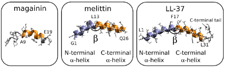
Figure 1: Structures of magainin Hara et al. (2001), melittin Terwilliger et al. (1982) and LL-37 Wang (2008). The melittin and LL-37 structures contain two $\alpha$-helices that form an angle $\beta$ (not the same for both structures). The $\alpha$-helices used in the analysis are colored in blue (N-terminal) and orange (C-terminal), with the limiting amino acids labeled on the structure. Side chain and non-helical residues are colored in gray.

The method is applied to three amphipathic antimicrobial model peptides: magainin, which is found in the skin of the African clawed frog Zasloff (1987), melittin, an active component in bee venom Habermann (1972), and LL-37, a peptide derived from the human protein cathelicidin which is involved in the innate immune defense system Gudmundsson et al. (1996). As shown in Fig. 1, the peptides vary in length and shape, and can thus be expected to display different sensing characteristics. Many antimicrobial peptides are believed to work by mediating membrane disruption Melo et al. (2009). The peptides studied here are thought to mediate the formation of toroidal membrane pores with a highly curved inner surface partly lined with lipids Ludtke et al. (1996); Yang et al. (2001); Leontiadou et al. (2006); Henzler Wildman et al. (2003); Anthony G. (2011); Sun et al. (2015), although the evidence appears less clear for LL-37 Wang et al. (2014). The ability to stabilize highly curved membrane structures suggests an intrinsic preference for curved membranes, as is generally expected for amphipathic peptides.

Our method uses simulated membrane buckling to sample the unconstrained interaction of single biomolecules with a range of membrane curvatures, and extends previous simulation studies of buckling mechanics Noguchi (2011); Hu et al. (2013), curvature-dependent folding and binding of amphipathic helices Cui et al. (2011), and lipid partitioning Wang (2008). We obtain joint distributions of peptide positions and orientations that yield new biophysical insights about curvature sensing. The three model peptides display similar rotation-averaged curvature preferences but differ in orientational preferences, which demonstrates the value of directional information. The asymmetry of the position-orientational distributions challenges continuum models of amphipathic helices as cylindrical membrane inclusions Campelo et al. (2008); Campelo and Kozlov (2014). We speculate that such asymmetry is important for certain modes of antibacterial activity, and argue that it might be common also for larger curvature sensing proteins. Finally, we discuss the limitations of characterizing curvature sensing mechanisms from assays with zero Gaussian curvature, and conclude that this uncertainty affects the overall binding energy, but not the orientational preferences. These results motivate efforts to track positions and orientations of membrane proteins experimentally, and to develop assays with a broader range of local curvatures.

Methods

To study curvature sensing by single peptides, we simulate their interactions with a buckled membrane using the coarse-grained Martini model Marrink et al. (2007), and track their position and orientation, as shown in Fig. 2. On a microscopic level, curvature sensing by amphipathic helices is associated with the density and size of bilayer surface defects Hatzakis et al. (2009a); Cui et al. (2011), which are well described by the Martini model Vanni et al. (2014).

Simulation parameters

We performed molecular dynamics simulations using Gromacs 4.6.1 Pronk et al. (2013), and the coarse-grained Martini force-field with polarizable water model Marrink et al. (2007); Monticelli et al. (2008); Yesylevskyy et al. (2010), and a relative dielectric constant of 2.5 (as recommended Yesylevskyy et al. (2010)). We used standard lipid parameters for 1-palmitoyl-2-oleoyl phosphatidylethanolamine (POPE) Marrink et al. (2004), 1-palmitoyl-2-oleoyl phosphatidylglycerol (POPG) Baoukina et al. (2007), and peptides de Jong et al. (2013). The peptide structures for magainin (PDB ID:1DUM), melittin (PDB ID:2MLT), and LL-37 (PDB ID: 2K6O) were obtained from the Protein Data Bank, and coarse-grained with the martinize script provided by the MARTINI developers. Constant temperature was maintained with the velocity rescaling thermostat Bussi et al. (2007) with a $1.0\text{\,}\mathrm{ps}$ time constant, and pressure was controlled with the Berendsen barostat Berendsen et al. (1984) using a time constant of $12\text{\,}\mathrm{ps}$ and a compressibility of $3\text{\times}{10}^{-4}\text{\,}{\mathrm{bar}}^{-1}$. Peptide (when present), lipids and solvent were coupled separately to the temperature bath. Coulomb interactions were modelled with the particle mesh Ewald method Essmann et al. (1995) setting the real-space cut-off to 1.4 nm and the Fourier grid spacing to 0.12 nm. Lennard-Jones interactions were shifted to zero between 0.9 and 1.2 nm. A time step of 25 fs was used in all simulations.

System assembly and membrane buckling

We assembled and equilibrated three rectangular ($L_{x}=2L_{y}$) bilayer patches of 1024 lipids each, with 70% POPE and 30% POPG, solvated with $\sim 21000$ coarse-grained water beads and neutralized with sodium ion beads. POPG is negatively charged, which promotes peptide binding. These patches were equilibrated for 25 ns in an NPT ensemble at 300 K and 1 bar, with pressure coupling applied semi-isotropically.

After equilibration, all systems were laterally compressed in the x direction by a factor $\gamma=(L-L_{x})/L=0.2$, where $L$ is the linear size of the flat system, and $L_{x}$ the size of the compressed simulation box, in the $x$ direction. This was done by scaling all $x$-coordinates, and the box size $L_{x}$, by a factor $1-\gamma=0.8$ at the end of the equilibration run, yielding $L_{x}=20.88$, 20.81 and 20.89 nm for the three patches, respectively. After rescaling, the compressibilities were set to 0 in the $x$ and $y$ directions to keep the system size constant in those directions for subsequent simulations. Pressure coupling was then applied anisotropically in the z direction only. We then performed an energy minimization and a short equilibration run (25 ns) to let the bilayer buckle.

Next, we added one peptide to each system, using the three independent patches to create three independent replicas for each peptide. The peptide was initially placed about 3 nm above the membrane surface, but quickly attached to the bilayer. After the binding event, we equilibrated the system for another $5\text{\,}\mathrm{\SIUnitSymbolMicro s}$ before starting a production run of $15\text{\,}\mathrm{\SIUnitSymbolMicro s}$, where we collected data every $5\text{\,}\mathrm{ns}$. All peptides remained essentially parallel to the membrane surface as expected , in agreement with experimental results for low peptide concentrations Hara et al. (2001); Terwilliger et al. (1982); Lee et al. (2013); Wang et al. (2014).

Membrane alignment and peptide tracking

The buckled membrane profile diffuses as a traveling wave the simulation (movie S1), but curvature sensing by a peptide is reflected in its distribution relative to the buckled shape. Hence, the buckled configurations must be aligned in order to extract useful information. To do this, we fit the $xz$-profile of the membrane by the ground state of the Helfrich model with periodic boundary conditions, which is one of the Euler buckling profiles of an elastic beam Noguchi (2011); Hu et al. (2013). This shape depends only on the dimensionless buckling parameter $\gamma$ ($\gamma=0$ is the flat state). Hence, if we compute the shape for some reference system, the general case can be obtained by shifting and scaling. We chose $L_{x}=1$ as reference, and write the buckling profile as a parametric curve $x=s+\xi(s,\gamma),z=\zeta(s,\gamma)$, parameterized by a normalized arclength coordinate $0<s<1$ (the absolute arclength is given by $sL=sL_{x}(1-\gamma)^{-1}$).

For fast evaluation, we expanded $\xi(s,\gamma)$ and $\zeta(s,\gamma)$ in truncated Fourier series in $s$, and created look-up tables for Fourier coefficients vs. $\gamma$. We defined $s$ to give the curve $z(x)$ a maximum at $s=0.5$, minima at $s=0,1$, and inflection points at $s=0.5\pm 0.25$, and aligned the buckled shapes by fitting the bilayer in each frame to the buckling profile and aligning the inflection points (Fig. 2, movies S2-S3). Specifically, we fit the rescaled buckling profile to the innermost tail beads of all lipids in each frame using least-squares in the $x$ and $z$ directions, i.e., minimizing

$$\sum_{i}(x_{0}+L_{x}\big{(}s+\xi(s_{i},\gamma)\big{)}-x_{i})^{2}+(z_{0}+L_{x}\zeta(s_{i},\gamma)-z_{i})^{2}$$ (1)

with respect to $\gamma$, the translations $x_{0},z_{0}$, and the normalized arc-length coordinates $s_{i}$ of each bead ($x_{i},z_{i}$ are bead positions). The time-averaged bilayer shape, after alignment, agrees well with the theoretical buckled shape (Fig. 3a).

The normalized arclength coordinate $s$ of the peptide was computed by projecting the peptide center of mass onto the buckled profile fitted to the membrane midplane. The in-plane orientation $\theta$ was then computed by fitting a line through the backbone particles of the $\alpha$-helical part of the peptide, projecting it onto the tangent plane at $s$, and computing the in-plane angle to the tangent vector $\mathbf{t}$ (see Fig. 2a). The local curvature at $s$, in the tangent direction of the buckled shape, is given by

$$C(s)=\frac{1-\gamma}{L_{x}}\frac{d\psi}{ds},$$ (2)

where $\psi$ is the bilayer mid-plane tangent angle of Fig. 2a,b Kreyszig (1991). (Note that the opposite sign convention is also common Zimmerberg and Kozlov (2006)) . In the theoretical analysis, we neglect small shape and area fluctuations ($\mathrm{std}(\gamma)\approx 0.005$) and use the nominal value $\gamma=0.2$.

Fitting

We used least-squares routines in MATLAB (MathWorks, Natick, MA) to fit the Boltzmann distributions $e^{-E(s_{i},\theta_{i})}/Z$ of the $E_{C}$ (Eq. 8) and $E_{2}$ (Table S1) models to $(s,\theta)$-histograms built from the aggregated data with 50 bins for each coordinate. Both data and model histograms were normalized numerically. Error bars in Fig. 4d are boot-strap standard deviations from 1000 bootstrap realizations, using blocks of length 100 (500 ns) as the elementary data unit for resampling Künsch (1989).

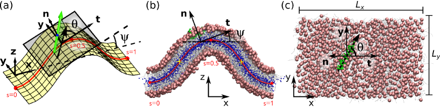
Figure 2: Buckled simulation and analysis. (a) The position $s$ of a peptide is defined by the projection of the center-of-mass (blue dot) onto the midplane surface (yellow). The in-plane orientation $\theta$ is defined by projecting the peptide backbone direction (green arrow, pointing towards the C-terminal end) onto the local tangent plane (gray) at $s$. The local tangent and normal vectors are indicated by t and n, respectively. (b) Side and (c) top view of a simulation snapshot with peptide position and orientation indicated using the notation and local coordinate system in (a). The system size is $L_{x}=20.88$ nm and $L_{y}=13.05$ nm. The peptide (LL-37 in this case) is shown in green, and lipids in gray (tails), light red (phosphate groups) and blue (innermost tail beads). The side view (b) also shows the Euler buckling profile (red line) fitted to the bilayer mid-plane, and the inflection points at $s=0.5\pm 0.25$ (yellow crosses) used to align the buckled configurations. Molecular graphics generated with VMD Humphrey et al. (1996).

Results

Preferred curvature and orientations

We simulated single peptides interacting with a buckled bilayer, using three independent production runs of 15 $\mu s$ for each peptide, and tracked their normalized arc-length coordinates $s\in[0,1]$ and in-plane orientations $\theta$ (Fig. 2a). Aggregated $(s,\theta)$-histograms are shown in Fig. 3b-d, and convergence is discussed in Sec. S1.

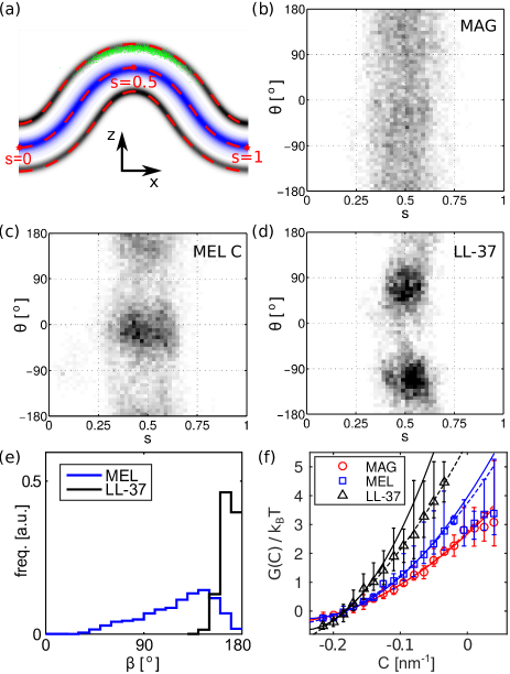
Figure 3: Distributions of peptide positions and orientations in the buckled bilayer. (a) Average buckled shape in terms of densities of inner lipid tail beads (blue) and phosphate groups (gray) after alignment, for one production run with LL-37. Green dots show representative peptide center-of-mass positions. Dashed red lines indicate the average fitted mid-plane $\pm 2.15$ nm offsets in the normal direction. (b-d) Aggregated $(s,\theta)$-histograms for (b) magainin, (c) melittin (using the orientation of the C-terminal helix), and (d) LL-37. (e) Distributions of internal angle $\beta$ (see Fig. 1) for melittin and LL-37. (f) Orientation-averaged binding free energy vs. curvature at the peptide center-of-mass (Eq. (4)) for the three peptides. Error bars show max and min values from three independent simulations. Dashed lines are guides to the eye (fits to quadratic curves), and solid lines are results for the $E_{C}$ model (Eq. (8)) using the fit parameters in Fig. 4.

All three peptides prefer the concave high curvature regions with a maximum at $s=0.5$, as expected for hydrophobic insertion mechanisms Campelo et al. (2008); Campelo and Kozlov (2014); Sodt and Pastor (2014); Hatzakis et al. (2009b); Cui et al. (2011); Vanni et al. (2014). Regarding the angle distributions, the three peptides behave differently. Magainin displays a rather uniform angle distribution, probably because its short $\alpha$-helical segment creates a fairly symmetric insertion footprint. For melittin, the joint between the N- and C-terminal helices appears very flexible, resulting in a broad distribution of the internal angle $\beta$ (Fig. 3e). Both helices prefer directions nearly parallel to the x-axis, the direction of maximum curvature, but the preference is stronger and slightly offset ($\theta_{max}\approx-15^{\circ},165^{\circ}$) for the C-terminal helix shown in Fig. 3c, while the N-terminal helix is more symmetrically oriented (Fig. S2).

LL-37 maintains a linear structure, and its $\theta$-distribution displays two sharp maxima near $\theta=70^{\circ}$ and $\theta=-110^{\circ}$ (Fig. 3d). This is remarkable since, by reflection symmetry around $s=0.5$, the curvatures in those directions are the same as along $-70^{\circ}$ and $110^{\circ}$, orientations that are clearly not preferred. As we will argue below, this can be understood as curvature sensing along directions different from that of the peptide itself. These sensing directions adopt $\theta=0,90^{\circ}$, and thus map onto themselves under reflection. Notably, none of the peptides orient directly along the flat direction $\theta=90^{\circ}$ as commonly assumed in mechanical models Campelo et al. (2008); Campelo and Kozlov (2014).

Orientation-averaged binding free energy

Next, we look at the orientation-averaged binding free energy, corresponding to the curvature-dependent enrichment measured in many in vitro assays Zhu et al. (2012); Sorre et al. (2012); Aimon et al. (2014); Shi and Baumgart (2015); Hsieh et al. (2012); Ramesh et al. (2013); Black et al. (2014). To extract the curvature dependence of the binding energy, we analyse center-of-mass positions along the buckled shape. These should follow a Boltzmann distribution, proportional to $e^{-G(s)}$, where $G(s)$ is the orientation-averaged binding free energy in units of $k_{B}T$. We model this as depending on the local curvature only, and hence set $G(s)=G(C(s))$, and extract $G(C)$ from curvature histograms, weighted according to the change-of-variable transformation that relates the density of curvatures, $\rho(C)$, to the density of positions $\rho(s)$. Indeed, dropping normalization constants, we have

$$\rho_{s}(s)ds\propto e^{-G(C(s))}ds\propto e^{-G(C)}|dC/ds|^{-1}dC\propto\rho_{C}(C)dC,$$ (3)

from which it follows that

$$G(C)=-\ln\big{(}\rho_{C}(C)|dC/ds|\big{)}+const.$$ (4)

The weights $|dC/ds|$ can be understood as compensating for the fact that not all curvatures have equal arclength footprints along the buckled profile. To estimate $G(C)$, we estimated $\rho(C)$ using a simple histogram, and the weights as the mean of $|dC/ds|$ for all contributions to each bin.

Fig. 3f shows the binding free energy profiles $G(C)$ for the different peptides, which are more similar than the $(\theta,s)$-distributions, and well fit by quadratic curves. Note that Eq. (4) does not yield absolute binding energies of the peptides, and the $G(C)$ curves are instead offset vertically for easy visualization. Experimental binding free energies of these peptides to flat membranes with anionic lipids range from -15 to -10 $k_{B}T$ He and Lazaridis (2013).

Quantitative models

We now turn to quantitative models of the peptides’ curvature sensing. As described in the introduction, we model the binding energy of a peptide as a function of the local curvature tensor in a frame rotating with the peptide, and treat the bilayer itself as having fixed shape and thus a fixed deformation energy which we neglect. Generally, if the principal curvatures and directions are $c_{1,2}$ and $\vec{e}_{1,2}$, the curvature tensor, or second fundamental form, in a frame rotated by an in-plane angle $\theta$ relative to $\vec{e}_{1}$, is given by

$$C_{ij}=\left[\begin{array}[]{cc}H\!\!+\!\!D\cos 2\theta&D\sin 2\theta\\ D\sin 2\theta&H\!\!-\!\!D\cos 2\theta\end{array}\right]=\left[\begin{array}[]{cc}C_{\parallel}&C_{X}\\ C_{X}&C_{\perp}\end{array}\right],$$ (5)

where $H=(c_{1}+c_{2})/2$ and $D=(c_{1}-c_{2})/2$ are the mean and deviatoric curvatures, and the Gaussian curvature is given by $K=c_{1}c_{2}=C_{\parallel}C_{\perp}-C_{X}^{2}$. Note the symmetry under rotations by $180^{\circ}$, since the curvature of a line is the same in both directions. For the buckled surface, $c_{1}=C(s),\,c_{2}=0$ (and hence $K=0$, $H=D=C(s)/2$), $\vec{e}_{1}=\mathbf{t}$, $\vec{e}_{2}=\mathbf{y}$. As shown in Fig. 2, we define the rotating frame using the peptide’s center of mass and the direction of the $\alpha$-helical parts, and thus $\theta$ is the peptide in-plane orientation, and $\parallel,\perp$ denote the longitudinal ($\theta$) and transverse ($\theta+90^{\circ}$) directions.

The simplest models are linear in $C_{ij}$, but can be ruled out since they cannot reproduce the convex binding free energies in Fig. 3f. To see this, we write a general linear model in the form $E_{1}=aH+bD\cos(2(\theta-\alpha))$ Fournier (1996), and integrate out the angular dependence to get

$$G_{1}=-\ln\int_{0}^{2\pi}e^{-E_{1}}d\theta=aH-\ln I_{0}(bD)+const.$$ (6)

Since $H=D=C(s)/2$ on the buckled surface, and the modified Bessel function $I_{0}$ is convex, $G_{1}$ will be either downward convex (if $b\neq 0$) or linear and direction insensitive (when $b\to 0$), in disagreement with Fig. 3.

Moving on to quadratic terms, Akabori and Santangelo Akabori and Santangelo (2011) explored a model of the form

$$E_{X}=\!\frac{k_{\parallel}}{2}(C_{\parallel}\!-C_{\parallel 0})^{2}\!\!+k_{X}(C_{X}-C_{X0})^{2}\!\!+\frac{k_{\perp}}{2}(C_{\perp}\!-C_{\perp 0})^{2},$$ (7)

where $C_{\parallel 0}$, $C_{X0}$ and $C_{\perp 0}$ are preferred curvatures. Further simplifications $k_{X}$=0 and $k_{X}$=$k_{\perp}$=0 have also been studied Perutková et al. (2010); Ramakrishnan et al. (2010, 2011, 2013). While these models can all display non-trivial behavior, $E_{X}$ is not the most general quadratic model, which would include all 9 linear and quadratic combinations of the three independent curvature tensor components. In particular, $E_{X}$ does not contain a simple preferred mean curvature as a special case, because $H=(C_{\parallel}+C_{\perp})/2$, and hence $(H-H_{0})^{2}$ contains a term $C_{\parallel}C_{\perp}$ which is absent in Eq. (7).

However, the general quadratic model is not identifiable on surfaces with only one non-zero principal curvature. This is because the Gaussian curvature $K$ is zero, and hence the model can only be specified up to a term proportional to $K$. Also, $E_{X}$ can then be made to behave as a mean curvature sensor, since all angular dependence cancels if $k_{\parallel}=k_{\perp}=k_{X}$, $C_{\parallel 0}=C_{\perp 0}$, and $C_{X0}=0$. These limitations apply to our buckled surface, as well as to tubular and plane-wave geometries used experimentally Sorre et al. (2012); Zhu et al. (2012); Hsieh et al. (2012); Ramesh et al. (2013); Black et al. (2014). A curvature sensing mechanism therefore cannot be completely characterized using such surfaces, but some conclusions can be drawn.

In particular, setting $k_{X}=0$ in Eq. (7) yields an intuitive model with curvature sensing only along the longitudinal and transverse directions Perutková et al. (2010); Ramakrishnan et al. (2010, 2011, 2013). From Eq. (5), this means angular dependence only in the form $\cos 2\theta$, which is symmetric around $\theta=0$, $\pm\frac{\pi}{2}$, and $\pm\pi$. However, the orientational distributions in Fig. 4a do not display this symmetry, although the statistics is not quite clear in the case of melittin (see Fig. S2). Apparently, the curvature sensing directions are not generally aligned with the actual helices. This resembles results for $\alpha$-synuclein, where peptides and induced membrane deformations appear similarly misaligned Braun et al. (2012). A simple quadratic model incorporating these observations is

$$E_{C}=\frac{\kappa}{2}(2H-C_{0})^{2}+bD\cos\big{(}2(\theta-\alpha)\big{)}+\kappa_{G}K,$$ (8)

where the Gaussian curvature coefficient $\kappa_{G}$ is unidentifiable since $K=0$ in our data. As shown in Fig. 4, $E_{C}$ describes all peptides reasonably well, and using the full quadratic model does not significantly improve the fit.

To better understand the physical meaning of this model, we explore some alternative formulations. First, using Eq. (5) to trade $H,D$ for the $C_{ij}$, and rearranging the terms, we find an equivalent formulation that resembles the $E_{X}$ model,

$$E_{C}^{\prime}=\frac{\kappa}{2}\big{(}C_{\parallel}-C_{0}+\frac{b}{2\kappa}\cos 2\alpha\big{)}^{2}+\kappa\big{(}C_{X}+\frac{b}{2\kappa}\sin 2\alpha\big{)}^{2}\\ +\frac{\kappa}{2}\big{(}C_{\perp}-C_{0}-\frac{b}{2\kappa}\cos 2\alpha\big{)}^{2}+(\kappa+\kappa_{G})K.$$ (9)

Continuing, we can rotate the basis attached to the peptide by $\alpha$, and thus generate a transformed curvature tensor with elements $C_{ij}^{(\alpha)}(\theta)=C_{ij}(\theta+\alpha)$ satisfying

$$C_{\parallel}^{(\alpha)}+C_{\perp}^{(\alpha)}=2H,\quad C_{\parallel}^{(\alpha)}-C_{\perp}^{(\alpha)}=2D\cos\big{(}2(\theta-\alpha)\big{)}.$$ (10)

In this basis, there is an $E_{X}$-like equivalent model that lacks ’off-diagonal’ elements,

$$E_{C}^{\prime\prime}=\frac{\kappa}{2}\big{(}C_{\parallel}^{(\alpha)}-C_{0}+\frac{b}{2\kappa}\big{)}^{2}+\frac{\kappa}{2}\big{(}C_{\perp}^{(\alpha)}-C_{0}-\frac{b}{2\kappa}\big{)}^{2}+(\kappa+\kappa_{G})K,$$ (11)

i.e., sensing curvature along two orthogonal directions that are rotated by an angle $\alpha$ with respect to the peptide backbone. Note that since Gaussian curvature is rotationally invariant, the unidentifiable Gaussian curvature term only affects the overall affinity to membranes with Gaussian curvature, and not the orientational preferences of the peptides.

As a consistency check, we integrated out $\theta$ from $E_{C}$. Proceeding as for $G_{1}$ in Eq. (6) and setting $H=D=C(s)/2$, $K=0$, we get

$$G_{C}=-\ln\int_{0}^{2\pi}d\theta e^{-E_{C}}=\frac{\kappa}{2}(C-C_{0})^{2}-\ln I_{0}\big{(}bC/2\big{)},$$ (12)

which we compare with $G(C)$ in Fig. 3f using the parameters of Fig. 4d. Magainin and melittin shows good agreement, but not LL-37, whose $(s,\theta)$-distribution (Fig. 3d) is also less symmetric around $s=0.5$ than expected from the symmetry of the buckled shape. A simple explanation is that the effective “sensing site” does not coincide with the center of mass used to define $s$. This is illustrated in Fig. 5 by a hypothetical peptide which is fixed at $s=0.5$ but free to rotate. As a result, the N-terminal end shows $(s,\theta)$-correlations resembling those seen for the LL-37 center of mass, indicating that its “sensing site” is located in the C-terminal part. Numerical experiments in Sec. S2 agree qualitatively with this geometric argument, and both symmetry and consistency improves when tracking the LL-37 C-terminal helix instead (but the fit parameters do not change significantly).

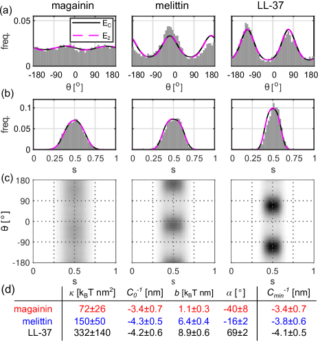
Figure 4: Fitting quadratic models to data. (a,b) marginal position and angle distributions, showing data (gray) and nearly identical curves from the $E_{C}$ and general quadratic model ($E_{2}$, see Table S1). (c) $(s,\theta)$-distributions for the $E_{C}$ model. (d) $E_{C}$ fit parameters $\pm$ bootstrap SEM Künsch (1989) due to finite sampling (see Sec. S1), with $\alpha$ indicating the preferred orientation. $C_{min}$ is the preferred curvature, from minimizing Eq. 12.

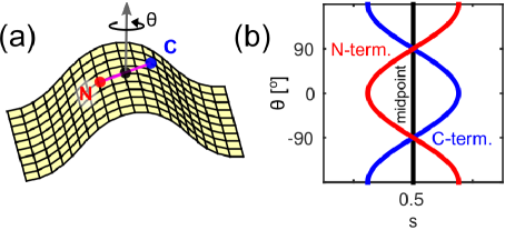
Figure 5: Curvature sensing site and $(s,\theta)$-correlations. (a) A freely rotating peptide whose midpoint (black) is fixed at $s=0$. (b) Resulting correlations $s_{C,N}\propto\pm\cos\theta$ for the N- and C-terminal ends (red,blue).

Discussion

We describe a simulation approach to study membrane curvature sensing by tracking positions and orientations of single molecules interacting with a buckled lipid bilayer. This approach is widely applicable, and the utility of angular information is obvious from the observation that the three peptides show distinct orientational distributions, but very similar orientation-averaged binding energy curves (Fig. 3).

Our data is well described by modelling the binding energy in terms of local curvatures, yielding more complex models than commonly used to fit orientation-averaged data Zhu et al. (2012); Sorre et al. (2012); Aimon et al. (2014); Shi and Baumgart (2015), and also less symmetric than some theoretical suggestions Perutková et al. (2010); Ramakrishnan et al. (2010, 2011, 2013). The observed asymmetry also seems difficult to reconcile with continuum elasticity models of hydrophobic insertion in terms of cylindrical membrane inclusions Campelo et al. (2008); Campelo and Kozlov (2014). Recently, continuum elasticity models were found to underpredict the induced curvature of a hydrophobic insertion compared to atomistic simulations Sodt and Pastor (2014). Our data shows an additional qualitative effect of molecular detail, which we believe reflect the fact that the mirror symmetry of cylinder-shaped inclusions is absent from the peptide structures. Instead, our data can be described in terms of curvature sensing directions that are not aligned with the inserted $\alpha$-helices. Since amphipathic helices are common curvature sensing motifs Drin et al. (2007) and mirror symmetry is generally absent also in multimeric proteins Goodsell and Olson (2000), such asymmetric sensing might be common.

These results should motivate efforts to track the position and orientation of membrane proteins experimentally, for example using polarization-based optical techniques Rosenberg et al. (2005) or electron microscopy Davies et al. (2012). It would also be valuable to vary mean and Gaussian curvatures independently in order to probe Gaussian curvature sensing, for example by extending supported bilayer assays with plane-wave surfacesHsieh et al. (2012) to shapes with non-zero Gaussian curvature. Another possibility might be to combine assays with cylindrical geometries ($K=0$), such as plane waves Hsieh et al. (2012) or membrane tethersZhu et al. (2012); Sorre et al. (2012); Aimon et al. (2014); Shi and Baumgart (2015); Ramesh et al. (2013) with spherical geometries ($K=H^{2}$) such as vesicles Hatzakis et al. (2009b); Tonnesen et al. (2014) or deposited nanoparticles Black et al. (2014).

An interesting aspect of the $E_{C}$ model is that it predicts a free energy minimum, i.e., a preferred curvature, at least when $K=0$ (Eq. 12). The preferred curvature radii $C_{\text{min}}^{-1}$ of our peptides, listed in Fig. 4c, are well above the monolayer thickness of about 2.2 nm (Fig. 3a) where the bilayer folds back on itself, but below the lowest radius in our simulations (about 4.5 nm), meaning that this prediction is somewhat speculative, since higher order terms might become important at very high curvatures. On a molecular level, curvature sensing by amphipathic peptides is thought to reflect an affinity for packing defects in the membrane-water interface Hatzakis et al. (2009b); Cui et al. (2011); Vanni et al. (2014). It is not clear that this mechanism predicts a preferred curvature at all. Testing this seems like an interesting question for future work.

Our results also have biophysical implications. At high concentrations, the three peptides are thought to mediate the formation of membrane pores with highly curved inner surfaces Ludtke et al. (1996); Yang et al. (2001); Leontiadou et al. (2006); Henzler Wildman et al. (2003); Anthony G. (2011); Sun et al. (2015). The orientational preferences we see in single peptides are consistent with atomistic Leontiadou et al. (2006) and coarse-grained Sun et al. (2015) simulations of multi-peptide pores. In particular, the asymmetric curvature preference of LL-37 should help select for a single handedness of the resulting tilted pore structure Sun et al. (2015), which might facilitate pore formation by reducing frustration. This mechanism may represent a general way for membrane proteins to induce a particular orientation or handedness in patterns on curved surfaces Mim et al. (2012).

Acknowledgments

We thank Astrid Gräslund, Oksana V. Manyuhina, Christoph A. Haselwandter, and two anonymous reviewers for helpful comments and discussions. Simulations were performed on resources provided by the Swedish National Infrastructure for Computing (SNIC) at the National Supercomputer Centre (NSC) and the High Performance Computing Center North (HPC2N). Financial support from the Wenner-Gren Foundations and the Swedish Foundation for Strategic Research (SSF) via the Center for Biomembrane Research are gratefully acknowledged.

Author contributions

JG and ML designed research. JG and FEW performed research. JG and ML analysed data. JG, FEW, and ML wrote the paper.

Anisotropic membrane curvature sensing by amphipathic peptides
– supporting information.

S1 Convergence and individual replicas

Simulations of proteins interacting with mixed bilayers can be challenging to converge due to slow lipid diffusion and long-lived protein-lipid interactions Ge et al. (2014). For this reason, we run three independent replicas rather than one long simulation for each peptide, and use them as a simple control of the robustness of our conclusions. Figures S1-S3 show histograms of center-of-mass positions, orientations, and joint positions-orientations of both the three individual production runs for each peptide, as well as aggregated histograms. In the case of melittin (Fig. S2), orientations of both the N- and C-terminal helices are shown.

While the results for individual trajectories are obviously noisier than the aggregated statistics, it is clear that the same qualitative features are present in all replicas. In particular, two well-separated orientational states of melittin and LL-37 are clearly visible (albeit not equally populated) in all trajectories, strongly indicating that our simulations are long enough to capture the major low-energy states of these systems. However, the sampling is still limited enough to induce significant statistical uncertainty in fit parameters, as seen Fig. 4d.

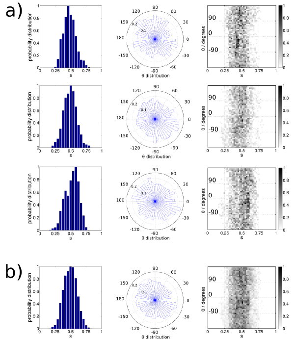
Figure S1: Results for magainin, from (a) three independent production runs, and (b) aggregated.

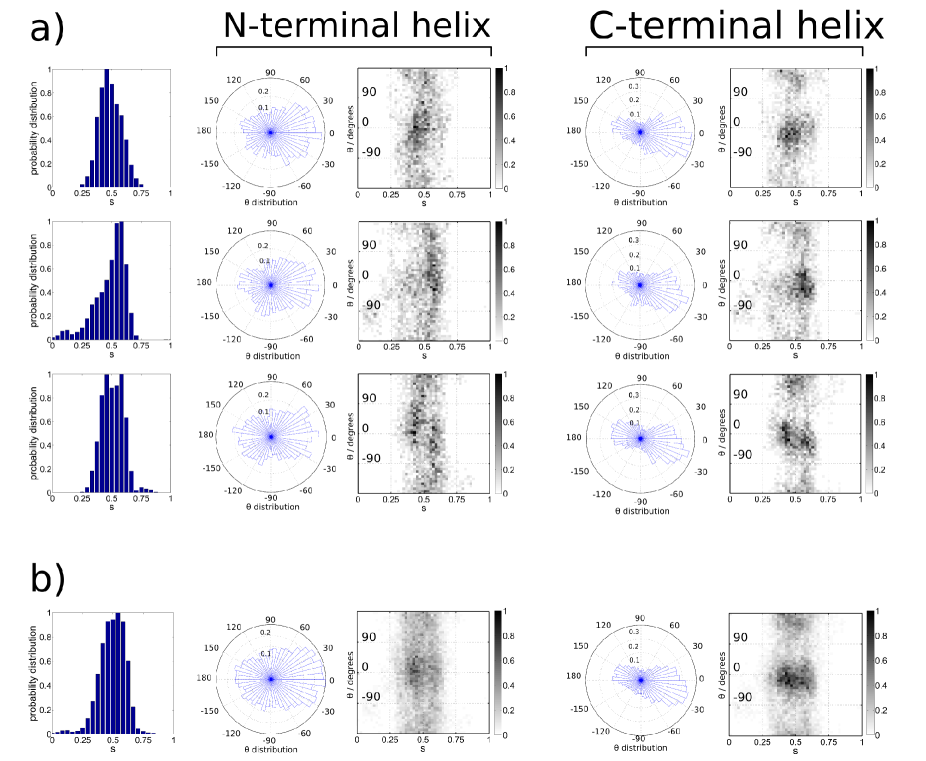
Figure S2: Results for melittin, from (a) the three independent production runs, and (b) aggregated. Both N- and C-terminal results are shown.

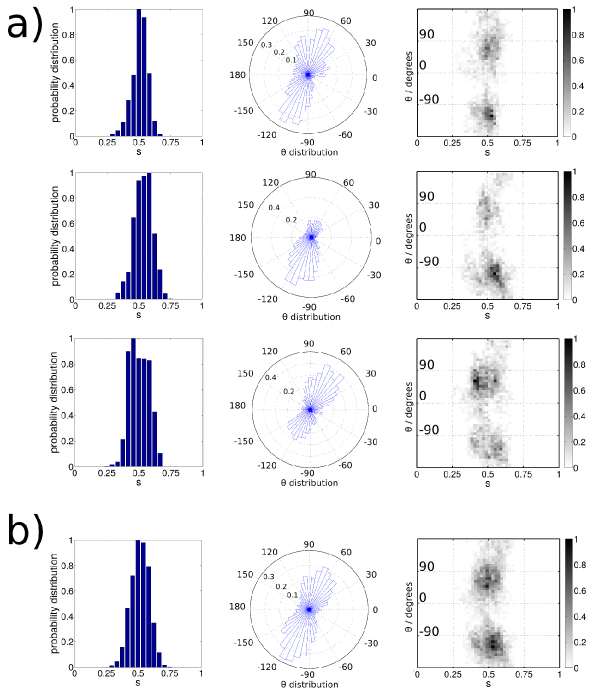
Figure S3: Results for LL-37, from (a) three independent production runs, and (b) aggregated.

Table S1: Fit parameters (fit$\pm$ bootstrap std.) for the $E_{2}$ model for the curves shown in Fig. 4, rounded to two significant digits, in appropriate units of $k_{B}T$ and nm. This model is given by $E_{2}=\frac{a_{1}}{2}(C_{\parallel}-a_{2})^{2}+a_{3}(C_{X}-a_{4})^{2}+\frac{a_{5}}{2}(C_{\perp}-a_{6})^{2}+a_{7}C_{X}(C_{\parallel}+C_{\perp})+a_{8}C_{X}(C_{\parallel}-C_{\perp}),$ i.e., with a $C_{\parallel}C_{\perp}$-term omitted for identifiability.

	$a_{1}$	$a_{2}$	$a_{3}$	$a_{4}$
MAG	$71\pm 30$	$-0.30\pm 0.26$	$73\pm 28$	$0.024\pm 0.028$
MEL	$170\pm 52$	$-0.23\pm 0.03$	$130\pm 52$	$0.002\pm 0.02$
LL-37	$300\pm 130$	$-0.24\pm 0.07$	$300\pm 140$	$-0.02\pm 0.03$
	$a_{5}$	$a_{6}$	$a_{7}$	$a_{8}$
MAG	$68\pm 28$	$-0.30\pm 0.27$	$-24\pm 19$	$5.3\pm 3.3$
MEL	$90\pm 55$	$-0.3\pm 1.3$	$27\pm 28$	$2.4\pm 4.2$
LL-37	$310\pm 150$	$-0.25\pm 0.73$	$68\pm 59$	$1\pm 7$

S2 Location of the curvature sensing site on LL-37

LL-37 shows indications of asymmetry around $s=0.5$ that is incompatible with the symmetry of the curvature tensor elements (Fig. 3d), and the fitted $E_{C}$ model is also less consistent with the orientation averaged binding energy (Fig. 3e) than the other peptides. Here, we explore the hypothesis that these effects are caused by using the center-of-mass of the peptide for defining the position $s$, which might be inappropriate if the sensitivity is unequally distributed along the peptide. Our rationale for this hypothesis is that a correlation between position and orientation, as indicated in the LL-37 data in Fig. 3d might come about if the effective curvature sensing site is different than the center-of-mass which we tracked to extract that data, as sketched in Fig. 5.

In Fig. S4, we show the corresponding analysis for LL-37 assuming a few alternative effective curvature sensing sites, with the center-of-mass in the middle row. The correlation between $\theta$ and $s$ around each peak clearly becomes more pronounced and N-terminal-like (c.f. Fig. 5) when the tracking site moves towards the N-terminal end. However, the asymmetry almost disappears when one assumes the effective curvature sensing site to be the center of mass of the C-terminal helix, and appears again with the opposite C-terminal-like trend when tracking the C-terminal end. Of these cases, the center-of-mass of the C-terminal helix is most consistent with the symmetries of curvature tensor elements and thus acts as an effective “sensing site”, which indicates that this part of the peptide is more important for curvature sensing. Fitting the $E_{C}$ model to this data yields $\kappa=323\pm 127\;k_{B}T\mathrm{nm}$, $C_{0}^{-1}=-4.1\pm 0.5$ nm, $b=8.2\pm 0.6$ k_BTnm, and $\alpha=69\pm 2^{\circ}$, not significantly different from the parameters shown in Fig. 4.

However, all distributions are still slightly asymmetric around $s=0.5$, with average $s$-values ranging from about 0.52 to 0.51 for the N- and C-terminal ends respectively, corresponding to an average displacement of 0.5 nm to 0.35 nm from the mid point. A closer examination of the significance of this observation would require substantially better statistics, perhaps from using some enhanced sampling method, as well as more systematic studies using a larger range of curvatures. This is outside the scope of this study.

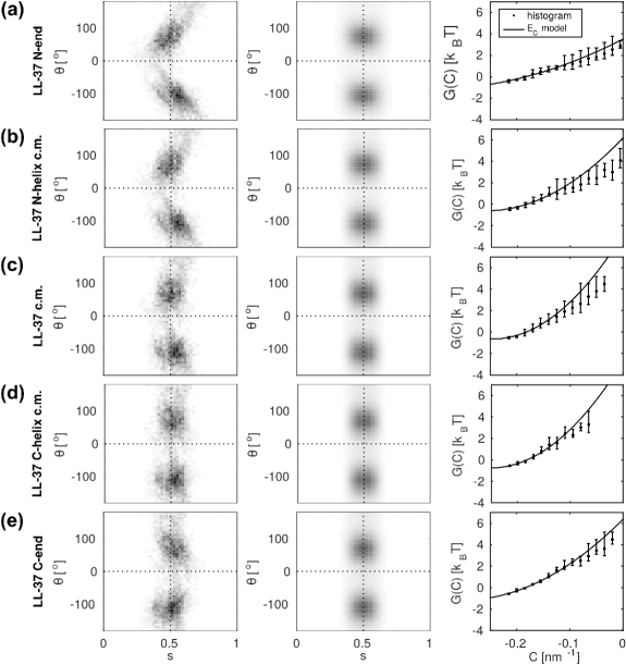
Figure S4: Analysis of LL-37 using different definitions of $s$ and $\theta$, namely (a) the first residue and orientation of the N-terminal helix, (b) the center-of-mass and orientation of the N-terminal helix, (c) the center-of-mass and orientation of the whole peptide (same as shown in the main text), (d) the center-of-mass and orientation of the C-terminal helix, and (e) the last residue and orientation of the C-terminal helix. relevant curvature sensing site. The columns show (left) the ($s,\theta$)-histogram, (mid) a fit of the $E_{C}$ model, and (right) the orientation-averaged binding free energy, obtained from the model fit (line) or using weighted histograms, Eq. 4, (dots) with error bars as in Fig. 3. The fit and histogram curves are vertically aligned by least-squares fit of the points at $C\leq-0.15$ ${\mathrm{nm}}^{-1}$.

References

- Zimmerberg and Kozlov (2006) Zimmerberg, J., and M. M. Kozlov, 2006. How proteins produce cellular membrane curvature. Nat. Rev. Mol. Cell Bio. 7:9–19.
- Baumgart et al. (2011) Baumgart, T., B. R. Capraro, C. Zhu, and S. L. Das, 2011. Thermodynamics and mechanics of membrane curvature generation and sensing by proteins and lipids. Annu. Rev. Phys. Chem. 62:483–506.
- Tonnesen et al. (2014) Tonnesen, A., S. M. Christensen, V. Tkach, and D. Stamou, 2014. Geometrical membrane curvature as an allosteric regulator of membrane protein structure and function. Biophys. J. 106:201–209.
- Engelman (2005) Engelman, D., 2005. Membranes are more mosaic than fluid. Nature 438:578–580.
- Fournier (1996) Fournier, J. B., 1996. Nontopological saddle-splay and curvature instabilities from anisotropic membrane inclusions. Phys. Rev. Lett. 76:4436–4439.
- Perutková et al. (2010) Perutková, Š., V. Kralj-Iglič, M. Frank, and A. Iglič, 2010. Mechanical stability of membrane nanotubular protrusions influenced by attachment of flexible rod-like proteins. J. Biomech. 43:1612–1617.
- Ramakrishnan et al. (2010) Ramakrishnan, N., P. B. Sunil Kumar, and J. H. Ipsen, 2010. Monte Carlo simulations of fluid vesicles with in-plane orientational ordering. Phys. Rev. E 81:041922.
- Ramakrishnan et al. (2011) Ramakrishnan, N., P. B. S. Kumar, and J. H. Ipsen, 2011. Modeling anisotropic elasticity of fluid membranes. Macromol. Theor. Simul. 20:446–450.
- Ramakrishnan et al. (2013) Ramakrishnan, N., P. B. Sunil Kumar, and J. H. Ipsen, 2013. Membrane-mediated aggregation of curvature-inducing nematogens and membrane tubulation. Biophys. J. 104:1018–1028.
- Akabori and Santangelo (2011) Akabori, K., and C. D. Santangelo, 2011. Membrane morphology induced by anisotropic proteins. Phys. Rev. E 84:061909.
- Walani et al. (2014) Walani, N., J. Torres, and A. Agrawal, 2014. Anisotropic spontaneous curvatures in lipid membranes. Phys. Rev. E 89:062715.
- Peter et al. (2004) Peter, B. J., H. M. Kent, I. G. Mills, Y. Vallis, P. J. G. Butler, P. R. Evans, and H. T. McMahon, 2004. BAR domains as sensors of membrane curvature: the amphiphysin BAR structure. Science 303:495–499.
- Blood and Voth (2006) Blood, P. D., and G. A. Voth, 2006. Direct observation of Bin/amphiphysin/Rvs (BAR) domain-induced membrane curvature by means of molecular dynamics simulations. Proc. Natl. Acad. Sci. U.S.A. 103:15068–15072.
- Drin et al. (2007) Drin, G., J.-F. Casella, R. Gautier, T. Boehmer, T. U. Schwartz, and B. Antonny, 2007. A general amphipathic -helical motif for sensing membrane curvature. Nat. Struct. Mol. Biol. 14:138–146.
- Campelo et al. (2008) Campelo, F., H. T. McMahon, and M. M. Kozlov, 2008. The hydrophobic insertion mechanism of membrane curvature generation by proteins. Biophys. J. 95:2325–2339.
- Campelo and Kozlov (2014) Campelo, F., and M. M. Kozlov, 2014. Sensing membrane stresses by protein insertions. PLoS Comput. Biol. 10:e1003556.
- Sodt and Pastor (2014) Sodt, A. J., and R. W. Pastor, 2014. Molecular modeling of lipid membrane curvature induction by a peptide: more than simply shape. Biophys. J. 106:1958–1969.
- Zhu et al. (2012) Zhu, C., S. L. Das, and T. Baumgart, 2012. Nonlinear sorting, curvature generation, and crowding of endophilin N-BAR on tubular membranes. Biophys. J. 102:1837–1845.
- Sorre et al. (2012) Sorre, B., A. Callan-Jones, J. Manzi, B. Goud, J. Prost, P. Bassereau, and A. Roux, 2012. Nature of curvature coupling of amphiphysin with membranes depends on its bound density. Proc. Natl. Acad. Sci. U.S.A. 109:173–178.
- Aimon et al. (2014) Aimon, S., A. Callan-Jones, A. Berthaud, M. Pinot, G. E. S. Toombes, and P. Bassereau, 2014. Membrane shape modulates transmembrane protein distribution. Dev. Cell 28:212–218.
- Shi and Baumgart (2015) Shi, Z., and T. Baumgart, 2015. Membrane tension and peripheral protein density mediate membrane shape transitions. Nat. Commun. 6:5974.
- Hsieh et al. (2012) Hsieh, W.-T., C.-J. Hsu, B. R. Capraro, T. Wu, C.-M. Chen, S. Yang, and T. Baumgart, 2012. Curvature sorting of peripheral proteins on solid-supported wavy membranes. Langmuir 28:12838–12843.
- Ramesh et al. (2013) Ramesh, P., Y. F. Baroji, S. N. S. Reihani, D. Stamou, L. B. Oddershede, and P. M. Bendix, 2013. FBAR syndapin 1 recognizes and stabilizes highly curved tubular membranes in a concentration dependent manner. Sci. Rep. 3:1565.
- Black et al. (2014) Black, J. C., P. P. Cheney, T. Campbell, and M. K. Knowles, 2014. Membrane curvature based lipid sorting using a nanoparticle patterned substrate. Soft Matter 10:2016.
- Zasloff (1987) Zasloff, M., 1987. Magainins, a class of antimicrobial peptides from Xenopus skin: isolation, characterization of two active forms, and partial cDNA sequence of a precursor. Proc. Natl. Acad. Sci. U.S.A. 84:5449–5453.
- Habermann (1972) Habermann, E., 1972. Bee and wasp venoms. Science 177:314–322.
- Gudmundsson et al. (1996) Gudmundsson, G. H., B. Agerberth, J. Odeberg, T. Bergman, B. Olsson, and R. Salcedo, 1996. The human gene FALL39 and processing of the cathelin precursor to the antibacterial peptide LL-37 in granulocytes. Eur. J. Biochem. 238:325–332.
- Melo et al. (2009) Melo, M. N., R. Ferre, and M. A. R. B. Castanho, 2009. Antimicrobial peptides: linking partition, activity and high membrane-bound concentrations. Nat. Rev. Microbiol. 7:245–250.
- Ludtke et al. (1996) Ludtke, S. J., K. He, W. T. Heller, T. A. Harroun, L. Yang, and H. W. Huang, 1996. Membrane Pores Induced by Magainin†. Biochemistry 35:13723–13728.
- Yang et al. (2001) Yang, L., T. A. Harroun, T. M. Weiss, L. Ding, and H. W. Huang, 2001. Barrel-stave model or toroidal model? A case study on melittin pores. Biophys. J. 81:1475–1485.
- Leontiadou et al. (2006) Leontiadou, H., A. E. Mark, and S. J. Marrink, 2006. Antimicrobial peptides in action. J. Am. Chem. Soc. 128:12156–12161.
- Henzler Wildman et al. (2003) Henzler Wildman, K. A., D.-K. Lee, and A. Ramamoorthy, 2003. Mechanism of lipid bilayer disruption by the human antimicrobial peptide, LL-37. Biochemistry 42:6545–6558.
- Anthony G. (2011) Anthony G., L., 2011. Biological membranes: the importance of molecular detail. Trends in Biochemical Sciences 36:493–500.
- Sun et al. (2015) Sun, D., J. Forsman, and C. E. Woodward, 2015. Amphipathic membrane-active peptides recognize and stabilize ruptured membrane pores: exploring cause and effect with coarse-grained simulations. Langmuir 31:752–761.
- Wang et al. (2014) Wang, G., B. Mishra, R. F. Epand, and R. M. Epand, 2014. High-quality 3D structures shine light on antibacterial, anti-biofilm and antiviral activities of human cathelicidin LL-37 and its fragments. BBA - Biomembranes 1838:2160–2172.
- Noguchi (2011) Noguchi, H., 2011. Anisotropic surface tension of buckled fluid membranes. Phys. Rev. E 83:061919.
- Hu et al. (2013) Hu, M., P. Diggins, and M. Deserno, 2013. Determining the bending modulus of a lipid membrane by simulating buckling. J. Chem. Phys. 138:214110–214110–13.
- Cui et al. (2011) Cui, H., E. Lyman, and G. A. Voth, 2011. Mechanism of membrane curvature sensing by amphipathic helix containing proteins. Biophys. J. 100:1271–1279.
- Wang (2008) Wang, G., 2008. Structures of human host defense cathelicidin LL-37 and its smallest antimicrobial peptide KR-12 in lipid micelles. J. Biol. Chem. 283:32637–32643. PDB: 2K6O.
- Hara et al. (2001) Hara, T., H. Kodama, M. Kondo, K. Wakamatsu, A. Takeda, T. Tachi, and K. Matsuzaki, 2001. Effects of peptide dimerization on pore formation: Antiparallel disulfide-dimerized magainin 2 analogue. Biopolymers 58:437–446. PDB: 1DUM.
- Terwilliger et al. (1982) Terwilliger, T. C., L. Weissman, and D. Eisenberg, 1982. The structure of melittin in the form I crystals and its implication for melittin’s lytic and surface activities. Biophys. J. 37:353–361. PDB: 2MLT.
- Marrink et al. (2007) Marrink, S. J., H. J. Risselada, S. Yefimov, D. P. Tieleman, and A. H. de Vries, 2007. The MARTINI force field: coarse grained model for biomolecular simulations. J. Phys. Chem. B 111:7812–7824.
- Hatzakis et al. (2009a) Hatzakis, N. S., V. K. Bhatia, J. Larsen, K. L. Madsen, P. Bolinger, A. H. Kunding, J. Castillo, U. Gether, P. Hedegård, and D. Stamou, 2009. How curved membranes recruit amphipathic helices and protein anchoring motifs. Nat. Chem. Biol. 5:835–841.
- Vanni et al. (2014) Vanni, S., H. Hirose, H. Barelli, B. Antonny, and R. Gautier, 2014. A sub-nanometre view of how membrane curvature and composition modulate lipid packing and protein recruitment. Nat. Commun. 5:4916.
- Pronk et al. (2013) Pronk, S., S. Páll, R. Schulz, P. Larsson, P. Bjelkmar, R. Apostolov, M. R. Shirts, J. C. Smith, P. M. Kasson, D. van der Spoel, B. Hess, and E. Lindahl, 2013. GROMACS 4.5: a high-throughput and highly parallel open source molecular simulation toolkit. Bioinformatics 29:845–854.
- Monticelli et al. (2008) Monticelli, L., S. K. Kandasamy, X. Periole, R. G. Larson, D. P. Tieleman, and S.-J. Marrink, 2008. The MARTINI coarse-grained force field: extension to proteins. J. Chem. Theory Comput. 4:819–834.
- Yesylevskyy et al. (2010) Yesylevskyy, S. O., L. V. Schäfer, D. Sengupta, and S. J. Marrink, 2010. Polarizable water model for the coarse-grained MARTINI force field. PLoS Comput. Biol. 6:e1000810.
- Marrink et al. (2004) Marrink, S. J., A. H. de Vries, and A. E. Mark, 2004. Coarse grained model for semiquantitative lipid simulations. J. Phys. Chem. B 108:750–760.
- Baoukina et al. (2007) Baoukina, S., L. Monticelli, M. Amrein, and D. P. Tieleman, 2007. The molecular mechanism of monolayer-bilayer transformations of lung surfactant from molecular dynamics simulations. Biophys. J. 93:3775–3782.
- de Jong et al. (2013) de Jong, D. H., G. Singh, W. F. D. Bennett, C. Arnarez, T. A. Wassenaar, L. V. Schäfer, X. Periole, D. P. Tieleman, and S. J. Marrink, 2013. Improved parameters for the Martini coarse-grained protein force field. J. Chem. Theory Comput. 9:687–697.
- Bussi et al. (2007) Bussi, G., D. Donadio, and M. Parrinello, 2007. Canonical sampling through velocity rescaling. J. Chem. Phys. 126:014101.
- Berendsen et al. (1984) Berendsen, H. J. C., J. P. M. Postma, W. F. van Gunsteren, A. DiNola, and J. R. Haak, 1984. Molecular dynamics with coupling to an external bath. J. Chem. Phys. 81:3684–3690.
- Essmann et al. (1995) Essmann, U., L. Perera, M. L. Berkowitz, T. Darden, H. Lee, and L. G. Pedersen, 1995. A smooth particle mesh Ewald method. J. Chem. Phys. 103:8577–8593.
- Lee et al. (2013) Lee, M.-T., T.-L. Sun, W.-C. Hung, and H. W. Huang, 2013. Process of inducing pores in membranes by melittin. Proc. Natl. Acad. Sci. U.S.A. 110:14243–14248.
- Kreyszig (1991) Kreyszig, E., 1991. Differential geometry. Dover Publications, New York.
- Künsch (1989) Künsch, H. R., 1989. The Jackknife and the Bootstrap for general stationary observations. Ann. Stat. 17:1217–1241.
- Humphrey et al. (1996) Humphrey, W., A. Dalke, and K. Schulten, 1996. VMD: Visual molecular dynamics. J. Mol. Graphics 14:33–38.
- Hatzakis et al. (2009b) Hatzakis, N. S., V. K. Bhatia, J. Larsen, K. L. Madsen, P.-Y. Bolinger, A. H. Kunding, J. Castillo, U. Gether, P. Hedegård, and D. Stamou, 2009. How curved membranes recruit amphipathic helices and protein anchoring motifs. Nat. Chem. Biol. 5:835–841.
- He and Lazaridis (2013) He, Y., and T. Lazaridis, 2013. Activity determinants of helical antimicrobial peptides: A large-scale computational study. PLoS ONE 8:e66440.
- Braun et al. (2012) Braun, A. R., E. Sevcsik, P. Chin, E. Rhoades, S. Tristram-Nagle, and J. N. Sachs, 2012. -Synuclein induces both positive mean curvature and negative Gaussian curvature in membranes. J. Am. Chem. Soc. 134:2613–2620.
- Goodsell and Olson (2000) Goodsell, D. S., and A. J. Olson, 2000. Structural symmetry and protein function. Annu. Rev. Biophys. Biomol. Struct. 29:105–153.
- Rosenberg et al. (2005) Rosenberg, S. A., M. E. Quinlan, J. N. Forkey, and Y. E. Goldman, 2005. Rotational motions of macromolecules by single-molecule fluorescence microscopy. Acc. Chem. Res. 38:583–593.
- Davies et al. (2012) Davies, K. M., C. Anselmi, I. Wittig, J. D. Faraldo-Gómez, and W. Kühlbrandt, 2012. Structure of the yeast F1Fo-ATP synthase dimer and its role in shaping the mitochondrial cristae. Proc. Natl. Acad. Sci. U.S.A. 19:13602–13607.
- Mim et al. (2012) Mim, C., H. Cui, J. A. Gawronski-Salerno, A. Frost, E. Lyman, G. A. Voth, and V. M. Unger, 2012. Structural basis of membrane bending by the N-BAR protein endophilin. Cell 149:137–145.
- Ge et al. (2014) Ge, C., J. Gómez-Llobregat, M. J. Skwark, J.-M. Ruysschaert, Å. Wieslander, and M. Lindén, 2014. Membrane remodeling capacity of a vesicle-inducing glycosyltransferase. FEBS J. 281:3667–3684.