Objective-oriented Persistent Homology

Abstract

Persistent homology provides a new approach for the topological simplification of big data via measuring the life time of intrinsic topological features in a filtration process and has found its success in scientific and engineering applications. However, such a success is essentially limited to qualitative data characterization, identification and analysis (CIA). Indeed, persistent homology has rarely been employed for quantitative modeling and prediction. Additionally, the present persistent homology is a passive tool, rather than a proactive technique, for CIA. In this work, we outline a general protocol to construct objective-oriented persistent homology methods. By means of differential geometry theory of surfaces, we construct an objective functional, namely, a surface free energy defined on the data of interest. The minimization of the objective functional leads to a Laplace-Beltrami operator which generates a multiscale representation of the initial data and offers an objective oriented filtration process. The resulting differential geometry based objective-oriented persistent homology is able to preserve desirable geometric features in the evolutionary filtration and enhances the corresponding topological persistence. The cubical complex based homology algorithm is employed in the present work to be compatible with the Cartesian representation of the Laplace-Beltrami flow. The proposed Laplace-Beltrami flow based persistent homology method is extensively validated. The consistence between Laplace-Beltrami flow based filtration and Euclidean distance based filtration is confirmed on the Vietoris-Rips complex for a large amount of numerical tests. The convergence and reliability of the present Laplace-Beltrami flow based cubical complex filtration approach are analyzed over various spatial and temporal mesh sizes. The Laplace-Beltrami flow based persistent homology approach is utilized to study the intrinsic topology of proteins and fullerene molecules. Based on a quantitative model which correlates the topological persistence of fullerene central cavity with the total curvature energy of the fullerene structure, the proposed method is used for the prediction of fullerene isomer stability. The efficiency and robustness of the present method are verified by more than 500 fullerene molecules. It is shown that the proposed persistent homology based quantitative model offers good predictions of total curvature energies for ten types of fullerene isomers. The present work offers the first example to design objective-oriented persistent homology to enhance or preserve desirable features in the original data during the filtration process and then automatically detect or extract the corresponding topological traits from the data.

Keywords:  Objective-oriented persistent homology, Differential geometry based persistent homology, Laplace-Beltrami flow based filtration, Objective-oriented partial differential equation, Protein, Fullerene, Total curvature energy.

I Introduction

In mathematical science, homology is a general procedure to associate a sequence of abelian groups or modules to a given topological space and/or manifold [39, 26]. The idea of homology dates back to Euler and Riemann, although homology class was first rigorously defined by Henri Poincaré, who built the foundation of the modern algebraic topology. The topological structure of a given manifold can be studied via defining the different dimensional homology groups on the manifold such that the bases of the homology groups are isomorphic to the bases of the corresponding topological spaces. In computational perspective, a given manifold can be approximated by the triangulated simplicial complex, on which homology groups can be further defined. The triangulation of a manifold or a topological space can be realized through a number of methods, such as Delaunay triangulation. There are many triangulation software packages, such as TetGen and CGAL. In scientific computing, the Cartesian representation is one of most important approaches in numerical analysis. Consequently, cubical complex based homology analysis has also become a popular research topic in the past decade. A systematic description of homology analysis in the cubical complex setting has been given by Kaczynski et al [42].

Persistent homology creates a multiscale representation of topological structures via a scale parameter relevant to topological events. The basic concept was introduced by Robins [61] and Frosini and Landi [29], independently. Edelsbrunner et al. [25] introduced first efficient algorithm for persistent homology analysis. The generalization of persistent homology was given by Zomorodian and Carlsson [95]. In the past decade, persistent homology has been developed as an efficient computational tool for the characterization, identification and analysis (CIA) of topological features in large data sets [25, 95, 96]. Topological persistence over the filtration process can be captured continuously over a range of spatial scales in persistent homology analysis. Unlike commonly used computational homology which results in truly metric free or coordinate free representations, persistent homology is able to embed geometric information to topological invariants so that the “birth” and “death” of isolated components, circles, rings, loops, pockets, voids or cavities at all geometric scales can be monitored by topological measurements. Compared with traditional computational topology [44, 87, 12] and/or computational homology, persistent homology inherently has an additional dimension, namely, the filtration parameter, which can be utilized to embed some crucial geometry or quantitative information into the topological invariants. Barcode representation has been proposed for the visualization of topological persistence [32], in which various horizontal line segments or bars are utilized to represent the persistence of the topological features. Efficient computational algorithms such as, pairing algorithm [25, 22], smith normal form [26, 95] and Morse reduction [37, 38, 72], have been proposed to track topological variations during the filtration process [7, 26, 22, 23, 50]. Some of these persistent homology algorithms have been implemented in many software packages, namely Perseus [52, 50], JavaPlex [71] and Dionysus. In the past few years, persistent homology has been applied to image analysis [9, 58, 67, 5], image retrieval [30], chaotic dynamics verification [49, 42], sensor network [66], complex network [45, 40], data analysis [8, 53, 73, 60, 47], computer vision [67], shape recognition [24] and computational biology [43, 21, 31, 85].

Nevertheless, the applications of persistent homology have been essentially limited to qualitative CIA. Indeed, there is little literature about the use of persistent homology as a quantitative tool, i.e., for mathematical modeling and physical prediction, to our best knowledge. Recently, we have introduced molecular topological fingerprints (MTFs) as an efficient approach for protein CIA [85]. We have also utilized MTFs to reveal quantitative structure-function relationships in protein folding, protein stability and protein flexibility [85].

In the past few decades, geometric analysis, which combines differential equations and differential geometry, has become a popular approach for data analysis, signal and image processing, surface generation and computer visualization [27, 33, 48, 56, 64, 65, 69, 89]. Geometric partial differential equations (PDEs) [83], i.e., the Laplace-Beltrami flows, are efficient apparatuses in applied mathematics and computer science [11, 20, 68]. Osher and Sethian [55, 65] have devised level set as a computational tool for solving geometric PDEs. An alternative approach is to make use of the Euler-Lagrange variation to derive a desirable set of geometric PDEs from a functional, such as a Mumford-Shah functional [51], for image or surface analysis [6, 10, 46, 57, 62, 63]. Wei introduced some of the first families of high-order geometric PDEs for image analysis in 1998 [77]. Mathematical analysis of high-order geometric PDEs was reported in the literature [34, 35, 86, 41]. Geometric PDE based high-pass filters was pioneered by Wei and Jia by coupling two nonlinear geometric PDEs [79]. Recently, this approach has been extended to a more general formalism, the PDE transform, for image and surface analysis [74, 75, 76, 92].

In 2005, the use of curvature-controlled PDEs for the construction of biomolecular surfaces was introduced for the first time in computational biophysics [80]. The geometric PDE was shown to provide a multiscale representation of biomolecular surfaces [80]. Based on differential geometry, Wei and coworkers introduced the first variational solvent-solute interface: the minimal molecular surface (MMS) for molecular surface representation in 2006 [2, 3, 4]. Since the surface free energy is the product of surface tension and surface area, the minimization of the surface free energy leads to the Laplace-Beltrami operator. One then obtains the Laplace-Beltrami flow by adopting an artificial time. The Laplace-Beltrami flow approach has been used to calculate both solvation energies and electrostatics of proteins [18, 4, 1]. We have proposed potential-driven geometric flows, which admit non-curvature-driven terms, for biomolecular surface construction subject to potential interactions [1]. While our approaches were employed by many others [19, 88, 90, 91] for molecular surface analysis, our curvature-controlled PDEs and the differential geometry based Laplace-Beltrami models [80, 2, 4, 1] are, to our knowledge, the first of their kind for biomolecular surface and electrostatics/solvation modeling.

Using the variational principle, Wei introduced differential geometry based multiscale models in 2009 [78]. The essential idea is to use the differential geometry theory of surfaces as a natural means to geometrically separate the macroscopic domain of the biomolecule from the microscopic domain of the solvent, and to dynamically couple the continuum treatment of the solvent from the discrete description of the biomolecule. In the past few years, differential geometry based multiscale models have been implemented for nonpolar solvation analysis [18], full solvation analysis [15, 16, 17], proton transport [13, 14], ion permeation across membrane channel proteins [93, 94, 82, 81, 59]. The performance of our methods has been extensively validated with experimental data, including solvation energies and current-voltage (I-V) curves.

In this work, we propose objective-oriented persistent homology methods to proactively extract desirable topological traits from biomolecular data. As a general procedure, we construct an objective functional to optimize desirable features in data. In our specific example, such an optimization is realized through a geometry-embedded filtration process and leads to an objective-oriented persistent homology method. As a proof of principle, we utilize differential geometry theory of surfaces to minimize the surface free energy, which results in an objective-oriented partial differential equation, i.e., the Laplace-Beltrami flow. The evolution of the Laplace-Beltrami flow creates a multiscale representation of a nano-bio object, which naturally constitutes a filtration and gives rise to a differential geometry based persistent homology method. The proposed differential geometry based persistent homology is utilized to analyze nano-bio data. The topological invariants of a given nano-bio object are extracted from the evolutionary profiles of the Laplace-Beltrami flow. Then topological persistence is analyzed to identify the intrinsic topological signature of a given data. Such information is further utilized to unveil quantitative topology-function relationships. It is well known that geometric PDEs can be designed to preserve certain geometric features in the time evolution [77]. Specifically, Laplace-Beltrami flow minimizes the mean curvature or surface area [4]. As a result, topological invariants computed from the geometric PDE based filtration enhance the corresponding features. This idea is potentially useful and powerful for automatic feature detection and extraction from big data.

The rest of this paper is organized as follows. In Section II, we give a brief introduction to the theory of Laplace-Beltrami flows for nano-bio systems, such as proteins and carbon fullerene molecules. A computational protocol, including numerical implementation, for integrating the evolution Laplace-Beltrami flow is described in detail. In Section III, the brief review of homology and persistent homology theories are given in the cubical complex setting. The construction of objective-orieted persistent homology is discussed in Section IV. As a specific example of this new method, we propose the Laplace-Beltrami flow based persistent homology. The validity of the proposed method is carefully carried out in Section V using carbon fullerene data. The consistence with radius based filtration and the numerical convergence are verified. The proposed method is applied to the CIA of proteins and fullerene molecules in Section VI. We consider the topological persistence of a beta barrel, which has an intrinsic ring structure. We demonstrate that the specific intrinsic feature of the beta barrel, namely the inner ring structure, is enhanced during the time evolution. Whereas, some undesirable topological feature due to the Vietoris-Rips complex can be effectively suppressed in the present approach. We further apply this differential geometry based persistent homology to the quantitative prediction of fullerene isomer total curvature energies. This paper ends with a conclusion.

II Laplace-Beltrami flows for nano-bio systems

In this section, we provide a brief summary of differential geometry based Laplace-Beltrami flows. To this end, we discuss differentiable manifold and curvature, and followed by the construction of Laplace-Beltrami operator using an objective functional. The implementation of the Laplace-Beltrami flow for biomolecular data is described in detail.

II.A Differentiable manifolds and curvatures

Consider an immersion of an open set $U\subset{\mathbb{R}}^{3}$ to ${\mathbb{R}}^{4}$ via a differentiable hypersurface element ${\bf f}:U\rightarrow{\mathbb{R}}^{4}$. Here the hypersurface element is a vector-valued $C^{2}$ function: ${\bf f}({\bf u})=(f_{1}(u),f_{2}(u),f_{3}(u),f_{4}(u))$ and ${\bf u}=(u_{1},u_{2},u_{3})\in U$.

Tangent vectors (or directional vectors) of ${\bf f}$ are ${\bf X}_{i}=\frac{\partial{\bf f}}{\partial u_{i}}$. The Jacobi matrix of the mapping ${\bf f}$ is given by $D{\bf f}=({\bf X}_{1},{\bf X}_{2},{\bf X}_{3})$.

As a symmetric and positive definite metric tensor of ${\bf f}$, the first fundamental form is ${\bf I}:=(g_{ij})=(D{\bf f})^{T}\cdot(D{\bf f})$, where matrix elements are $g_{ij}=<{\bf X}_{i},{\bf X}_{j}>$. Here $<,>$ is the Euclidean inner product in ${\mathbb{R}}^{4}$, $i,j=1,2,3$.

The Gauss map $\nu:U\rightarrow S^{3}$ is defined by the unit normal vector $\nu({\bf u})$

$$\nu(u_{1},u_{2},u_{3}):=\frac{{\bf X}_{1}\times{\bf X}_{2}\times{\bf X}_{3}}{\|{\bf X}_{1}\times{\bf X}_{2}\times{\bf X}_{3}\|}\in\bot_{u}{\bf f},$$ (1)

where the cross product in ${\mathbb{R}}^{4}$ is a generalization of that in ${\mathbb{R}}^{3}$. Here $\bot_{u}{\bf f}$ is the normal space of ${\bf f}$ at point ${\bf p}={\bf f}({\bf u})$. It is easy to verify that

$$<\nu,\nu>=1.$$

Locally at ${\bf p}$, the normal vector $\nu$ is perpendicular to the tangent hyperplane $T_{u}{\bf f}$:

$$<\nu,{\bf X}>=0.$$

Note that $T_{u}{\bf f}\oplus\bot_{u}{\bf f}=T_{{\bf f}({\bf u})}{\mathbb{R}}^{3}$, which is the tangent space at point ${\bf p}$. The second fundamental form is of crucial importance and can be defined by means of the normal vector $\nu$ and tangent vector ${\bf X}_{i}$,

$${\bf II}({\bf X}_{i},{\bf X}_{j})=(h_{ij})\equiv\left(\left<-\frac{\partial\nu}{\partial u_{i}},{\bf X}_{j}\right>\right).$$ (2)

The definition of the second fundamental form can be systematically generalized by using the Weingarten map, a shape operator of ${\bf f}$:

$${\cal L}:=-D\nu\circ(D{\bf f})^{-1}.$$

Since ${\cal L}$ is a self-adjoint operator, we have

$${\bf II}({\bf X}_{i},{\bf X}_{j})={\bf I}({\cal L}{\bf X}_{i},{\bf X}_{j})=(h_{ij})=\left(\left<-\frac{\partial\nu}{\partial u_{i}},{\bf X}_{j}\right>\right)=\left(\left<\frac{\partial^{2}{\bf f}}{\partial u_{i}\partial u_{j}},\nu\right>\right).$$ (3)

The third and fourth fundamental forms are conveniently given in terms of the shape operator

$${\bf III}({\bf X}_{i},{\bf X}_{j}) = {\bf I}({\cal L}^{2}{\bf X}_{i},{\bf X}_{j})=(e_{ij})=\left(\left<\frac{\partial\nu}{\partial u_{i}},\frac{\partial\nu}{\partial u_{j}}\right>\right)$$ (4)

$${\bf IV}({\bf X}_{i},{\bf X}_{j}) = {\bf I}({\cal L}^{3}{\bf X}_{i},{\bf X}_{j}).$$ (5)

The Laplace-Beltrami can be calculated by

$$H=\frac{1}{3}h_{ij}g^{ji},$$ (6)

where we use the Einstein summation convention, and $(g^{ij})$ denotes the inverse matrix $(g^{ij})=(g_{ij})^{-1}$.

Principal curvatures $\kappa_{i}~{}(i=1,2,3)$ are defined as the eigenvalues of Weingarten map ${\cal L}$ with eigenvectors being unit tangent vectors. Appropriate organization of the principal curvatures gives rise to the first three Laplace-Beltramis

$$K_{1} = \frac{1}{3}(\kappa_{1}+\kappa_{2}+\kappa_{3})$$ (7)

$$K_{2} = \frac{1}{3}(\kappa_{1}\kappa_{2}+\kappa_{1}\kappa_{3}+\kappa_{2}\kappa_{3})$$ (8)

$$K_{3} = \kappa_{1}\kappa_{2}\kappa_{3}$$ (9)

where $K_{1}=H=\frac{1}{3}{\rm Tr}({\cal L})$ is the Laplace-Beltrami and $K_{3}=K={\rm Det}({\cal L})$ is the Gauss-Kronecker curvature or Gauss curvature. The local property of the Gauss curvature is used to classify the point as elliptic, hyperbolic, parabolic, etc. The combination of Gauss and Laplace-Beltramis has been used to characterize protein surfaces and predict protein-ligand binding sites [28, 84]. It follows from the Cayley-Hamilton theorem that the first four fundamental forms satisfy: ${\bf IV}-3H{\bf III}+3K_{2}{\bf II}-K{\bf I}=0$.

We discuss an iterative procedure to generate a family of hypersurfaces that have vanishing Laplace-Beltrami except at the boundary. Let $U\subset{\mathbb{R}}^{3}$ be an open set with a compact closure $\overline{U}$ and boundary $\partial U$. Consider a family of hypersurface elements ${\bf f}_{\varepsilon}:\overline{U}\rightarrow{\mathbb{R}}^{4}$ ($\varepsilon>0$) generated by deforming ${\bf f}$ in the normal direction with speed of the Laplace-Beltrami:

$${\bf f}_{\varepsilon}(x,y,z):={\bf f}(x,y,z)+\varepsilon H\nu(x,y,z).$$ (10)

Equation (10) is iterated until $H=0$ in all of $U$, except at boundary $\partial U$, which can be a set of atomic surface constraints. This procedure leads to a minimal hypersurface [4].

As discussed above, the hypersurface element is a vector-valued function which is cumbersome in biophysical application. We therefore construct a scalar hypersurface function by setting ${\bf f}({\bf u})=(x,y,z,S)$, where $S(x,y,z)$ is a hypersurface function of interest. The first fundamental form can be explicitly computed

$$(g_{ij})=\left(\begin{array}[]{lll}1+S_{x}^{2}&S_{x}S_{y}&S_{x}S_{z}\\ S_{x}S_{y}&1+S_{y}^{2}&S_{y}S_{z}\\ S_{x}S_{z}&S_{y}S_{z}&1+S_{z}^{2}\end{array}\right).$$ (11)

Matrix tensor $(g_{ij})$ has the inverse

$$(g^{ij})=\frac{1}{g}\left(\begin{array}[]{lll}1+S_{y}^{2}+S_{z}^{2}&-S_{x}S_{y}&-S_{x}S_{z}\\ -S_{x}S_{y}&1+S_{x}^{2}+S_{z}^{2}&-S_{y}S_{z}\\ -S_{x}S_{z}&-S_{y}S_{z}&1+S_{x}^{2}+S_{y}^{2}\end{array}\right),$$ (12)

where $g={\rm Det}(g_{ij})=1+S_{x}^{2}+S_{y}^{2}+S_{x}^{2}$ is the Gram determinant. From Eq. (1), the normal vector is given by

$$\nu=(-S_{x},-S_{y},-S_{z},1)/\sqrt{g}.$$ (13)

The second fundamental form, the Hessian matrix of $S$, is obtained as

$$(h_{ij})=\left(\frac{1}{\sqrt{g}}S_{x_{i}x_{j}}\right).$$ (14)

Using Eq. (6), one can obtain the Laplace-Beltrami

$$H=\frac{1}{3}\nabla\cdot\left(\frac{\nabla S}{\sqrt{g}}\right).$$ (15)

II.B Laplace-Beltrami flow

II.B.1 Laplace-Beltrami equation

According to differential geometry theory of surfaces, a surface area is minimized if and only if the Laplace-Beltrami is zero everywhere on the surface except for a set of boundary points. Following Eq. (10), we construct a family of hypersurfaces $S_{\varepsilon}$ as

$$S_{\varepsilon}(x,y,z)=S(x,y,z)+\frac{\varepsilon}{3\sqrt{g}}\nabla\cdot\left(\frac{\nabla S}{\sqrt{g}}\right).$$ (16)

The iteration of the hypersurface function so that $S_{\varepsilon}(x,y,z)\rightarrow S(x,y,z)$, i.e., $\nabla\cdot\left(\frac{\nabla S}{\sqrt{g}}\right)=0$, leads to the desired minimal hypersurface function $S$.

A more general procedure is to construct an objective functional, i.e., a surface free energy functional, for the molecular data of interest

$$E=\int_{\partial\Omega}\gamma d\Omega,$$ (17)

where $\partial\Omega$ is the boundary of the molecule, $\gamma$ is the surface tension and $d\Omega=\sqrt{g}dxdydz$. Using the Euler Lagrange equation, we minimize the surface free energy density $e=\gamma\sqrt{g}$ with respect to $S$

$$\frac{\partial e}{\partial S}-\frac{\partial}{\partial x}\frac{\partial e}{\partial S_{x}}-\frac{\partial}{\partial y}\frac{\partial e}{\partial S_{y}}-\frac{\partial}{\partial z}\frac{\partial e}{\partial S_{z}}=0.$$ (18)

Since $\gamma\neq 0$ in general, we arrive at the vanishing of the mean curvature operator $\nabla\cdot\left(\frac{\nabla S}{\sqrt{g}}\right)=3H=0$ again.

From the computational point of view, the iteration process can be efficiently achieved by introducing an artificial time variable $t$ so as to change the elliptic PDE into a parabolic one. Specifically, instead of iterating Eq. (16), we set the hypersurface function $S$ to be $S(x,y,z,t)$ in the computational perspective and construct the following Laplace-Beltrami equation

$$\frac{\partial S}{\partial t}=\sqrt{g}\nabla\cdot\left(\frac{\nabla S}{\sqrt{g}}\right).$$ (19)

A similar approach is to set $\sqrt{g}$ as $|\nabla S|$, leading to another popular form of the Laplace-Beltrami equation [4]

$$\frac{\partial S}{\partial t}=|\nabla S|\nabla\cdot\left(\frac{\nabla S}{|\nabla S|}\right).$$ (20)

These equations were employed to construct minimal molecular surfaces of proteins and other biomolecules [4, 1, 15, 84].

II.B.2 Initial value and boundary condition for nano-bio Laplace-Beltrami flows

In the present work, we generate a family of hypersurface functions indexed by the artificial time $t$ by using Laplace-Beltrami equataion (19). We call this family of hypersurface functions the profiles of Laplace-Beltrami flows. Note that we do not seek the minimal molecular surfaces described in our earlier work [4, 1, 15, 84]. Instead, we look for a geometric PDE or Laplace-Beltrami flow representation of nano-bio molecules. To apply this approach to proteins and nano-molecules, we start with a given set of $N$ atomic coordinates $\{{\bf r}_{i}\},~{}(i=1,2,\cdots,N)$, which can be obtained from Protein Data Bank (PDB) available on web or from the literature. We define a set by ${\bf R}_{N}=\cup_{i=1}^{N}B_{\epsilon}(r_{i})$, where $B_{\epsilon}({\bf r}_{i},r_{i})$ is the ball centered at ${\bf r}_{i}$ of radius $r_{i}=\varepsilon r_{vdW}$. Here $\epsilon>0$ is a parameter and $r_{vdW}$ is the van der Waals radius of the $i$th atom.

The initial value of the hypersurface $S$ can be chosen in a number of ways. One choice is

$$S({\bf r},0)=\begin{cases}1&\mbox{if ${\bf r}\in{\bf R}_{N}$},\\ 0&\mbox{otherwise}.\end{cases}$$ (21)

Remark 1.

The initial radius of an atom $\epsilon r_{i}$ in a molecule can be adjusted by parameter $\varepsilon$. For different applications, one can choose different initial radius. In our earlier work, $\epsilon>1$ was used [4, 1, 15, 84]. In the present work, we set $\epsilon=\frac{1}{2}$.

Alternatively, another choice is a heaviside function $\theta$

$$S({\bf r},0)=\theta(\mu({\bf r})-\mu_{0}),$$ (22)

where $\mu_{0}$ is a cutoff value and $\mu({\bf r})$ is a rigidity function [54]

$$\mu({\bf r})=\sum_{i}^{N}w_{i}\Phi(|{\bf r}-{\bf r}_{i}|;\eta_{i}).$$ (23)

Here $w_{i}$ is a weight associated with the atomic type of the $i$th atom and is set to 1 in the present work. Additionally, correlation function $\Phi(|{\bf r}-{\bf r}_{i}|;\eta_{i})$ is monotonically decreasing radial basis functions, such as generalized exponential functions or generalized Lorentz functions [54]. The scaling function $\eta_{i}$ can be set to $\eta_{i}\propto r_{\rm vdW}$ and should be systematically adjusted for different choices of $\Phi$.

Obviously, the other choice of the initial value is to directly use the rigidity function

$$S({\bf r},0)=\mu({\bf r}).$$ (24)

The initial values given by Eq. (22) are smoother than those given by Eq. (21). However, Eq. (24) provides the smoothest initial values. The results reported in this work are based on Eq. (21). However, our tests indicate that other two types of initial values work well.

Both the Dirichlet boundary ($S({\bf r},t)=0~{}\forall{\bf r}\in\partial U)$ or the Neumann boundary ($\frac{\partial S}{\partial{\bf r}}=0~{}\forall{\bf r}\in\partial U$) can be employed. The solution of Eq. (19) gives a family of hypersurface functions $S(x,y,z,t)$. We extract desirable nano-bio information from $S$ by using two different procedures. One is to take an iso-surface for a given iso-value, i.e., $S=c$, which can be extracted by the level set method. For our applications, the iso-value of the hypersurface for carbon fullerene molecules is set to be $c=0.1$, and that for protein molecules is set $c=0.01$. The other approach is to evaluate the structural information contained in $S(x,y,z,T)$ at a given time $T>>0$. We typically set $T$ to be a quite large value so the hypersurface profile is well developed. However, to avoid boundary effect, $T$ should not be too large.

III Cubical complex based homology and persistent homology

In this section, a brief review of the homology and persistent homology in the cubical complex setting is provided. The reader is referred to the literature [42, 70] for more comprehensive discussion and treatment.

III.A Geometric building blocks

The cubes are the basic geometric building blocks of the homology and persistent homology theory in the cubical complex setting. First of all, we need to introduce a few basic concepts about cubes.

• An elementary non-degenerate interval is a closed interval $I\subset\mathbb{R}$ of the form $I=[m,m+1]$ (or $I=[m]$ for simplicity) for some integer $m$. An elementary degenerate interval is a point $I=[m,m]$.

• An elementary cube $Q$ or $d$ cube is a $d$-product of elementary intervals, i.e.,

  $$Q=I_{1}\times I_{2}\times...\times I_{d}\subset\mathbb{R}^{d},$$

  where each $I_{i},i=1,2,...,d$ is an elementary interval of non-degenerated or degenerated type, and $d$ is called the embedding number of $Q$, denoted as ${\rm emb}~{}Q=d$. The dimension of $Q$, denoted by ${\rm dim}~{}Q$, is defined to be the number of non-degenerated components in $Q$, and $\mathcal{K}_{k}$ denotes the set of all $k$ dimensional elementary cubes. Let $\mathcal{K}:=\bigcup_{d=1}^{\infty}\mathcal{K}^{d}$ be the set of all elementary cubes, and $\mathcal{K}^{d}$ be the set of all elementary cubes in $\mathbb{R}^{d}$.

• The set of $k$-dim cubes with embedding number $d$ is $\mathcal{K}_{k}^{d}:=\mathcal{K}_{k}\bigcap\mathcal{K}^{d}$. Obviously, if $Q\in\mathcal{K}_{k}^{d}$ and $P\in\mathcal{K}_{k^{\prime}}^{d^{\prime}}$, then $Q\times P\in\mathcal{K}_{k+k^{\prime}}^{d+d^{\prime}}$.

With the above building blocks, we say that set $X\subset\mathbb{R}^{d}$ is cubical if $X$ can be written as a finite union of elementary cubes.

For a given cubical set $X\subset\mathbb{R}^{d}$, we define the following cubical set $\mathcal{K}(X)$ and $k$-cube set $\mathcal{K}_{k}(X)$ of $X$:

$$\mathcal{K}(X)=\{Q\in\mathcal{K}|Q\subset X\},$$

$$\mathcal{K}_{k}(X):=\{Q\in\mathcal{K}(X)|{\rm dim}~{}Q=k\}.$$

The elements of $\mathcal{K}_{k}(X)$ are called the $k$-cube of $X$.

III.B Algebraic building blocks

With the above geometric building blocks, we define the algebraic operations on the building blocks, following the line of Kaczynski et al. [42]

First, each elementary $k$-cube $Q\in\mathcal{K}_{k}^{d}$ is associated with an algebraic object $\hat{Q}$ which is called an elementary $k$-chain of $\mathbb{R}^{d}$. The set of all elementary $k$-chains of $\mathbb{R}^{d}$ is

$$\hat{\mathcal{K}}_{k}^{d}:=\{\hat{Q}|Q\in\mathcal{K}_{k}^{d}\},$$

and the set of all elementary chains of $\mathbb{R}^{d}$ is

$$\hat{\mathcal{K}}^{d}:=\bigcup_{k=0}^{\infty}\hat{\mathcal{K}}_{k}^{d}.$$

Second, addition operation and boundary operator are defined for the further algebraic treatment of the cubical complex.

III.B.1 Addition operation

To define the addition operation on elementary chains, first, the following $k$-chains, i.e., a linear combination of $k$-chain,

$$c=a_{1}\widehat{Q_{1}}+a_{2}\widehat{Q_{2}}+\cdots a_{m}\widehat{Q_{m}},\ \ a_{i}\in\mathbb{Z},i=1,2,...,m,$$

is allowed for any given finite collection $\{\widehat{Q_{1}},\widehat{Q_{2}},...,\widehat{Q_{m}}\}$, and, if all the $a_{i}=0$, then we set $c=0$.

The set of all the above $k$-chains is denoted by $C_{k}^{d}$. The addition of two $k$-chains is defined by:

$$\sum a_{i}\widehat{Q_{i}}+\sum b_{i}\widehat{Q_{i}}=\sum(a_{i}+b_{i})\widehat{Q_{i}}.$$

It is easy to check for $\forall$ $k$-chains $c=\sum_{i=0}^{m}a_{i}\widehat{Q_{i}}$, there is an inverse element $-c=\sum_{i=0}^{m}-a_{i}\widehat{Q_{i}}$ with the property $c+(-c)=0$, note the addition operation is commutable, thus $C_{k}^{d}$ is an abelian group.

III.B.2 Boundary operator

Before we define the boundary operator, the scalar product and cubical product operation on the $k$-chain group $C_{k}^{d}$ need to be defined.

Definition III.1.

Let $c_{1},c_{2}\in C_{k}^{d}$, where $c_{1}=\sum_{i=1}^{m}a_{i}\widehat{Q_{i}}$ and $c_{2}=\sum_{i=1}^{m}b_{i}\widehat{Q_{i}}$. The scalar product of chains $c_{1}$ and $c_{2}$ is defined as [42]:

$$<c_{1},c_{2}>:=\sum_{i=1}^{m}a_{i}b_{i}.$$

Definition III.2.

For all elementary cubes $P\in\mathcal{K}_{k}^{d}$ and $Q\in\mathcal{K}_{k^{\prime}}^{d^{\prime}}$, the cubical product between $P,Q$ is defined to be [42]:

$$\widehat{P}*\widehat{Q}:=\widehat{P\times Q}.$$

And for all chains $c_{1}\in C_{k}^{d}$ and $c_{2}\in C_{k^{\prime}}^{d^{\prime}}$, the cubical product is:

$$c_{1}*c_{2}=\sum_{P\in\mathcal{K}_{k},Q\in\mathcal{K}_{k^{\prime}}}<c_{1},\widehat{P}><c_{2},\widehat{Q}>\widehat{P\times Q},$$

and $c_{1}*c_{2}\in C_{k+k^{\prime}}^{d+d^{\prime}}$.

For the cubical product, the following important factorization property holds [42]:

Lemma III.1.

For $\forall\widehat{Q}\in\widehat{\mathcal{K}}^{d}$ with $d>1$. There exists unique elementary cubical chains $\widehat{I}$ and $\widehat{P}$ with ${\rm emb}~{}I=1$ and ${\rm emb}~{}P=d-1$, such that $\widehat{Q}=\widehat{I}*\widehat{P}$.

With the above preparation, the boundary operation can be defined inductively in the following way [42].

Definition III.3.

For $k\in\mathbb{Z}$, the cubical boundary operator

$$\partial_{k}:\mathcal{C}_{k}^{n}\rightarrow\mathcal{C}_{k-1}^{n}$$

is a homomorphism of abelian groups, defined for an elementary chain $\widehat{Q}\in\widehat{\mathcal{K}}_{k}^{n}$ by induction on the embedding number $n$ as follows:

• For $n=1$ $Q$ is an elementary interval, i.e., $Q=[m]$ or $Q=[m,m+1]$ for some $m\in\mathbb{Z}$, and one defines:

  $$\partial_{k}\widehat{Q}=\begin{cases}0&\mbox{if $Q=[m]$}\\ \widehat{[m+1]}-\widehat{[m]}&\mbox{if $Q=[m,m+1]$}.\end{cases}$$

• For $n>1$, let $I=I_{1}(Q)$ and $P=I_{2}(Q)\times\cdots\times I_{n}(Q)$ so that $\widehat{Q}=\widehat{I}*\widehat{P}$, then one defines:

  $$\partial_{k}\widehat{Q}=\partial_{{\rm dim}~{}I}\widehat{I}*\widehat{P}+(-1)^{{\rm dim}~{}I}\widehat{I}*\partial_{{\rm dim}~{}P}\widehat{P}.$$

By linearity this can be extended to chains, i.e., if $c=\sum_{i=1}^{p}a_{i}\widehat{Q}_{i}$, then:

$$\partial_{k}c=\sum_{i=1}^{p}a_{i}\partial_{k}\widehat{Q}_{i}.$$

Theorem III.1.

The boundary operator operator satisfies:

$$\partial_{k}\circ\partial_{k-1}=0,\ \ \forall k>1,$$

which is consistent with the simplicial complex setting.

Now, for a given cubical set $X\subset\mathbb{R}^{d}$, let $\{\widehat{K}_{k}(X):={\widehat{Q}|Q\in\mathcal{K}_{k}(X)}\}$ and let $C_{k}(X)$ be the subgroup of $C_{k}^{d}$ generated by the elements of $\widehat{K}_{k}(X)$, which is called the set of $k$-chains of $X$. The boundary operator maps $C_{k}(X)$ to a subset of $C_{k-1}(X)$, thus one can restrict the boundary operator to the cubical set $X$.

Definition III.4.

The boundary operator for the cubical set $X$ is defined to be:

$$\partial_{k}^{X}:C_{k}(X)\rightarrow C_{k-1}(X),$$

obtained by restricting $\partial_{k}:C_{k}^{d}\rightarrow C_{k-1}^{d}$ to $C_{k}(X)$.

Definition III.5.

The cubical chain complex for the cubical set $X\subset\mathbb{R}^{d}$ is

$$\mathcal{C}(X):=\{C_{k}(X),\partial_{k}^{X}\}_{k\in\mathbb{Z}},$$

where $C_{k}(X)$ are the groups of cubical $k$-chains generated by $\mathcal{K}_{k}(X)$ and $\partial_{k}^{X}$ is the cubical boundary operator restricted to $X$.

III.C Homology of cubical sets

As discussed above, one has the corresponding $k$-chains group $C_{k}(X)$, for a given cubical set $X$, now one can define two subgroups of $C_{k}(X)$.

• $k$-cycle group $Z_{k}(X):={\rm ker}~{}\partial_{k}^{X}=C_{k}(X)\bigcap{\rm ker}~{}\partial_{k}\subset C_{k}(X)$.

• $k$-boundary group $B_{k}(X):={\rm im}~{}\partial_{k+1}^{X}=\partial_{k+1}(C_{k+1}(X))\subset C_{k}(X)$.

Following from $\partial_{k}\circ\partial_{k-1}=0\ \ \forall k>1$, one has $B_{k}(X)\subset Z_{k}(X)$. Therefore, one has the following homology group [42].

Definition III.6.

The $k$th homology group of the cubical set $X$ is the quotient group:

$$H_{k}(X):=Z_{k}(X)/B_{k}(X).$$

The $k$th Betti number is defined as the rank of the $k$th homology group,

$$\beta_{k}={\rm rank}~{}H_{k}.$$

From the topological point of view, $H_{k}(X)$ describes $k$-dimensional holes of $X$, e.g., $H_{0}(X)$ measures connected components, $H_{1}(X)$ measures loops and $H_{2}(X)$ measures voids. In other words, $\beta_{0}$ is the number of connected components, $\beta_{1}$ is the number of loops, $\beta_{2}$ is the number of voids, and so on. We are particularly interested in behavior of $\beta_{0}$, $\beta_{1}$ and $\beta_{2}$ for proteins and fullerenes.

III.D Persistent homology of cubical complex

Homology gives a characterization of a manifold, while it does not distinguish different holes in the same dimension. To measure these topological features, the concept of persistent homology was proposed based on the simplicial complex. Persistence measures the birth, death and the lifetime of the topological attributes during the filtration process.

To define the persistent homology, first we need a filtration, i.e., a complex $K$ together with a nested sequence of sub-complexes $\{K^{i}\}_{0\leq i\leq n}$, such that

$$\emptyset=K^{0}\subset K^{1}\subset\cdots\subset K^{n}=K.$$

Each sub-complex $K^{i}$ in the filtration has an associated chain group $C_{k}^{i}$, cycle group $Z_{k}^{i}$ and boundary group $B_{k}^{i}$ $\forall i\geq 1$, and thus one has the following definition [70].

Definition III.7.

The $p$-persistent $k$th homology group of $K^{i}$ is:

$$H_{k}^{i,p}=Z_{k}^{i}/\left(B_{k}^{i+p}\bigcap Z_{k}^{i}\right).$$

Here $H_{k}^{i,p}$ captures the topological features of the filtrated complex that persists for at least $p$ steps in the filtration.

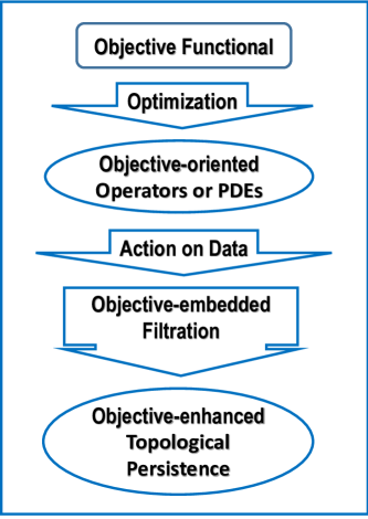
Figure 1: A flow chart for the construction of objective-oriented persistent homology.

IV Objective-oriented persistent homology

In this section, we propose a general procedure for constructing objective-oriented persistent homology. We start with an objective functional for the data of interest. By the optimization of the objective functional, we arrive at one or a set of objective-oriented operators, or objective-oriented PDEs. The number of operators depends on how the objective functional is parametrized. The action of the objective operators leads to a series of objective-embedded representations of the original data. We then utilize such objective-embedded representations for the filtration of original data to construct objective-oriented persistent homology. We illustrate this procedure by a flow chart in Fig. 1

As discussed in Section II.B, the minimization of the surface free energy functional gives rise to the mean curvature operator for the biomolecular data. We formulate the Laplace-Beltrami flow to computationally minimize the surface free energy. The integration of the Laplace-Beltrami flow leads to a family of minimal surface representations of the original data. In this part, we construct a filtration $\{K_{T}\}_{T\geq 1}$ of the data of interest based on the Laplace-Beltrami flow. Here, $T=0,1,2,\cdots,$ is the time steps. For a given initial structure, we embed it in an enlarged bounding box, which defines the whole computational domain. Then uniform Cartesian mesh is employed for our computation:

$$\{(i,j,k)|1\leq i\leq n_{x},1\leq j\leq n_{y},1\leq k\leq n_{z}\}.$$

The initial values of the grid points that is inside the initial geometric object is set to be $1$, and $0$ for grid points outside the object.

Under the geometric flow action, the following vertex set can be constructed at each evolution time:

$$V_{0}:=\emptyset,$$

$$V_{t}:=\{(i,j,k)|S(i,j,k,t)\geq S_{0},1\leq i\leq n_{x},1\leq j\leq n_{y},1\leq k\leq n_{z}\},\ \ \forall t>0,$$

where $S_{0}$ is the threshold value for extracting the iso-surface.

Furthermore, let $\tilde{V}_{T}:=\bigcup_{0\leq t\leq T}V_{t}$, which is the set of vertices that have value greater than the threshold value at time $T$.

The $T$th component of the filtration is set to be:

$$K_{T}:=\{\mbox{cubes whose vertices set is a subset of}\ \tilde{V}_{T}\}.$$

Based on the above construction, it is obvious that $K_{T}\subset K_{T+1},\forall~{}T\geq 0$.

Remark 2.

Neumann boundary condition is utilized to make the Laplace-Beltrami flow computationally well posed. Since the Laplace-Beltrami flow is dispersive, when the evolution time is large enough, the value of $S$ will be less than a given $S_{0}$ for all the grid points. Therefore the evolutionary flow based filtration is upper bounded.

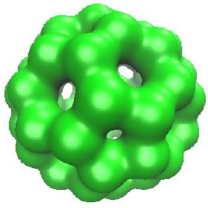
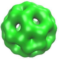
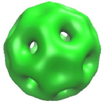
Figure 2: Selected frames of fullerene C₆₀ generated from the time evolution of the Laplace-Beltrami flow. Charts from left to right and from top to bottom are frames 1 to 6, respectively. According to Table 1, the second last frame has a central cavity while the last frame has no void.

IV.A Laplace-Beltrami flow based persistent homology

IV.B Computing Laplace-Beltrami flow based persistent homology

The objective-oriented persistent homology on the cubical complex can be computed by existing software packages. In the present work, we utilize Perseus [50] for persistent homology calculation. The sparse grid data structure is utilized as the input data format for the Perseus software in the present work.

Remark 3.

Since the Laplace-Beltrami flow minimizes the surface area of the surface defined on the initial data, the persistence of topological features associated with minimal surfaces is enhanced in the Laplace-Beltrami flow based persistent homology approach.

V Validation

V.A Topological invariant analysis

In this subsection, we examine accuracy and reliability of the proposed geometric flow based persistent homology method. To this end, we consider a fullerene molecule, C₆₀, which has distinct topological loops, namely pentagon and hexagon loops. The structural data of fullerene molecules and isomer total curvature energies [36] used in our tests are downloaded from the webpage: fullerene-isomers. In these structural data, coordinates of fullerene carbon atoms and isomer total curvature energies are given. The atoms of all these molecules form only two types of polygons, namely, pentagons and hexagons. For the fullerene cage composed only pentagons and hexagons, according to Euler Characteristics, the number of pentagons must be $12$ and that for hexagons is $\frac{N}{2}-10$, where $N$ is the number of atoms of the fullerene molecule.

Table 1: The evolution of the topological features of C₆₀ molecule under the time evolution of the Laplace-Beltrami flow.

Frame	Time	$\beta_{0}$	$\beta_{1}$	$\beta_{2}$
1	0.01	1	31	0
2	0.07	1	30	0
3	0.15	1	19	0
4	0.57	1	18	0
5	0.67	1	0	1
6	2.31	1	0	0

Figure 2 depicts six frames extracted from the solution of the Laplace-Beltrami equation for C₆₀ fullerene molecule. Note that the initial setting is a set of balls with half van der Waals radii as described in Eq. (21). It is seen that during the time evolution, many pentagonal rings disappear and followed by the disappearance of hexagonal rings. Table 1 gives a summary of topological invariants in these six frames. From this table we notice that pentagons persist in the time interval $[0,0.15]$ and the hexagon persist in the time interval $[0,0.67]$. The difference of the last two frames is that the second last frame has a cavity, whereas the last frame has no cavity.

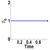
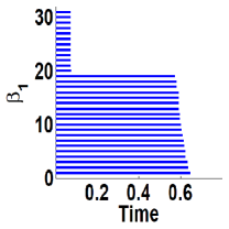
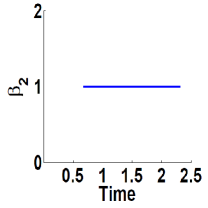
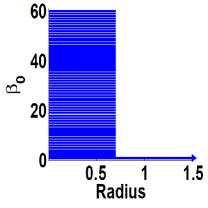
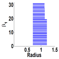
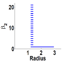
Figure 3: Comparison of the topological evolution and persistence of the C₆₀ molecule. Top row: Barcodes obtained from the proposed Laplace-Beltrami flow based filtration; Bottom row: Barcodes obtained from the Rips complex filtration.

The evolution of the topological features of carbon fullerene C₆₀ under the geometric flow is demonstrated in Fig. 3. As a comparison, we also plot the result generated by using the Rips complex. In $\beta_{0}$ panels, one sees a long-lasting bar from the present method, while a reduction from 60 bars to one bar in the Rips complex representation. This behavior is expected because the starting point of the present method is a set of connected balls as described above, while Rips complex filtration starts from the zero radius. In the $\beta_{1}$ panels, there is a good consistence between two approaches. One sees 12 short-lived bars, which correspond to 12 pentagonal rings. However, there are only 19 relatively long bars for 20 hexagonal rings because one of $H_{1}$ element can be expressed as the combination of other $H_{1}$ basis elements. Finally, in $\beta_{2}$ panels, the present method provides a single relatively long-lived bar for the inner cavity, while the Rips complex filtration gives rise to additional 20 short-lived bars for 20 hexagons. The disappearance of the short-lived $\beta_{2}$ bars in the present approach is due to the cubical complex used in our calculation. Short-lived bars are often regarded as topological noise in the literature, while used in our models for physical modeling [85]. However, in the present work, we only need the long-lasting $\beta_{2}$ bar for our quantitative modeling as discussed in Section VI.B.

Remark 4.

The persistent homology derived from the Laplace-Beltrami flow results in nonlinear modification of certain topological features. Because the geometric PDE is able to preserve certain geometric features [77], the persistence of the corresponding intrinsic topology can be amplified. This feature is a fundamental property of the objective-oriented persistent homology constructed in this work. It is possible to design objective-oriented PDEs to selectively enhance and/or extract other desirable topological features from big data.

V.B Convergence analysis

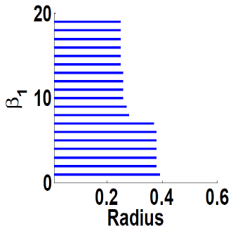
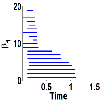
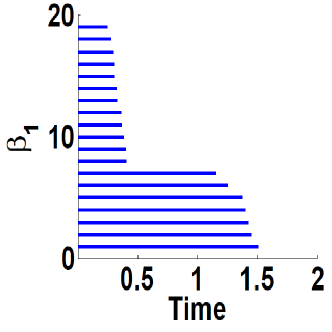
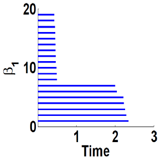
Figure 4: Comparison of the persistence of $\beta_{1}$ barcodes obtained from the growth of atomic radius filtration and from the geometric flow based filtration for fullerene C₃₆. Top left: Atomic radius filtration; Top right: Geometric flow filtration, $h=0.5$Å; Bottom left: Geometric flow filtration, $h=0.25$Å; Bottom right: Geometric flow filtration, $h=0.125$Å.

Figures 4 and 5 demonstrate the numerical convergence of of proposed Laplace-Beltrami flow approach for computing the persistence of $\beta_{1}$ invariants. We present the time evolution of the persistence of $\beta_{1}$ invariants collected over a sufficiently long period at different grid sizes. It can be seen that the persistent pattern at grid size $0.25$Å  is essentially the same as that at grid size $0.125$Å, which shows the convergence with respect to grid spacing variations.

As another validation of the proposed Laplace-Beltrami flow based persistent homology method, we examine the numerical convergence of the proposed method. Additionally, we demonstrate that topological invariants computed from our Laplace-Beltrami flow method converge to the right ones, where we regard the $\beta_{1}$ barcodes obtained via the conventional Rips complex filtration based on the growth of the radius of the point cloud data as the benchmark. To this end, we consider the persistent homology of the two approaches for two fullerene structures, namely, C₃₆ and C₁₀₀. The coordinates of these fullerene structures are downloaded from Web fullerene-isomers and are saved. For isomers, the first structure in the isomer family is used. These fullerene molecules contain pentagon and hexagon loops, which give rise to appropriate $\beta_{1}$ bars.

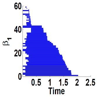
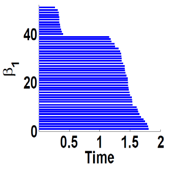
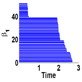
Figure 5: Comparison of the persistence of $\beta_{1}$ barcodes obtained from the growth of atomic radius filtration and from the geometric flow based filtration for fullerene C₁₀₀. Top left: Atomic radius filtration; Top right: Geometric flow filtration, $h=0.5$Å; Bottom left: Geometric flow filtration, $h=0.25$Å; Bottom right: Geometric flow filtration, $h=0.125$Å.

It remains to show that our persistent homology results converge to the right ones. As shown in Figures 4 and 5, there are a total of 12 pentagon $\beta_{1}$ bars. The numbers of hexagon bars are 7 and 39, respectively for C₃₆ and C₁₀₀, as expected. Therefore, the proposed geometric flow based filtration captures the intrinsic topological features of fullerenes. Additionally, the Rips complex based filtration is employed as a reference with a fine atomic radius growth rate of 0.001Å  per step. The comparison of topological invariants computed from the proposed method and that obtained from the Rips complex is given in Figures 4-5. Clearly, persistent patterns obtained by Laplace-Beltrami flow based method capture all topological features generated from the Rips complex, which indicates the reliability of the proposed method.

In fact, we have carried out similar tests for many other fullerenes, including C₃₈, C₄₀, C₄₄, C₅₂, C₈₄, C₈₆, C₉₀ and C₉₂. Although these results are omitted for simplicity, our findings are the same.

The above validations verify that the Laplace-Beltrami flow based filtration in conjugation with the cubical complex setting is convergent and accurate. The resulting topological invariants are consistent with those obtained with the Rips complex using radius based filtration. On the other hand, our results also indicate that the Laplace-Beltrami flow based method is very sensitive to grid resolution. Some topological features barely show up at the grid size of 0.5Å. Therefore, the grid resolution better than 0.25Å  is recommended for nano-bio data.

VI Application

Having verified the reliability, accuracy and efficiency of the present Laplace-Beltrami flow based persistent homology analysis, we utilize it for the study of proteins and nano-material in this section.

VI.A Protein structure analysis

VI.A.1 Protein 2GR8

In this subsection, we explore the topological structures and their persistence of the protein molecules using the Laplace-Beltrami flow based persistent homology. We consider a beta-barrel protein (PDB ID: 2GR8).

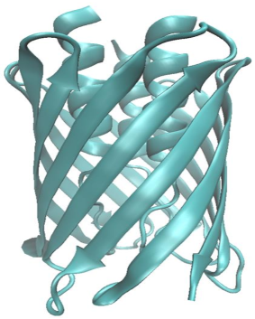
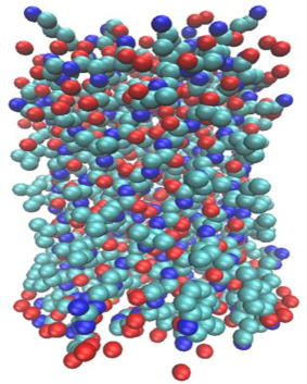
Figure 6: The initial structure of protein 2GR8. Left chart: Secondary structure representation; Right chart: atomic representation. Colors indicate different types of atoms.

Figure 6 shows the initial structure of protein 2GR8 in both secondary structure and atomic representations. Clearly, it is a beta barrel with 12 twisted beta strands coiled together in an antiparallel fashion to form a cylindrical structure in which the first strand is hydrogen bonded to the last. However, inside the beta barrel, there are also three alpha helices as shown in the left chart of Fig. 6. The topological structure is complicated due to the presence of these alpha helices.

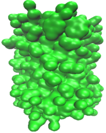
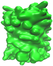
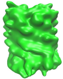
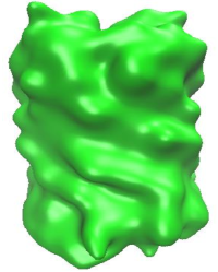
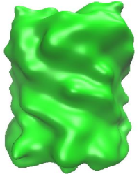
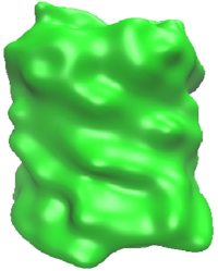
Figure 7: Geometric evolution of protein 2GR8 under the Laplace-Beltrami flow. Charts from left to right and from top to bottom are frames 1 to 6, respectively.

We first consider the geometric evolution of protein 2GR8 under the Laplace-Beltrami flow and then compute its homology evolution. Figure 7 depicts some frames generated from the time evolution process of the Laplace-Beltrami flow. The first two frames exhibit much atomic detail. As time progress, the atomic features disappear while beta strands are clearly demonstrated in frames 3-6. In fact, beta strand features diminish at the last two frames and the global cylindrical feature dominates. Therefore, the Laplace-Beltrami flow generates a multiscale representation of the protein as illustrated in our earlier work [80, 84].

Table 2: The time evolution of the topological invariants of protein 2GR8 under the Laplace-Beltrami flow.

Frame	Time	$\beta_{0}$	$\beta_{1}$	$\beta_{2}$
1	0.10	1	263	12
2	0.50	1	1	21
3	1.00	1	1	9
4	1.50	1	1	2
5	1.70	1	1	1
6	1.80	1	0	0

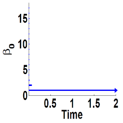
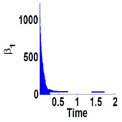
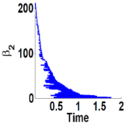
Figure 8: The time evolution of the topological invariants of protein 2GR8 under the Laplace-Beltrami flow.

Table 2 gives the corresponding time evolution of topological invariants of the six frames for protein 2GR8. One sees a large number of $\beta_{1}$ rings in the first frame. However, there is just one ring, in the second frame. The number of cavities reaches the highest values in the second frame (among six frames) and gradually reduces to zero. From Table 2, we note that there is a ring in Frames 2-5. However, we cannot determine whether it is the same ring or not from the classical homology theory. There may be a different ring generated at each of Frame 2-5. Persistent homology is designed to reserve this issue. The persistence of the topological invariants during the time evolution process is illustrated in Fig. 8. It is confirmed that the ring initially exists and is not generated in intermediate steps of the evolution. However, this ring is not a global one because it lasts for a relatively short period during the time evolution.

VI.A.2 A beta barrel

We next create a pure beta barrel by removing three alpha helices from protein 2GR8, which enables us to observe the beta barrel ring geometry and topology clearly. The initial structure of the beta barrel is shown in Fig. 9. The time evolution of the beta barrel is illustrated in Fig. 10. Again, one sees atomic details in the first few frames and global features in late frames. Obviously, there is a large ring structure in the beta barrel.

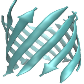
Figure 9: The initial structure of a beta barrel. Left chart: Secondary structure representation; Right chart: atomic representation. Colors indicate different types of atoms.

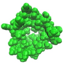
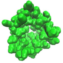
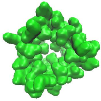
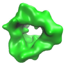
Figure 10: The geometric evolution of a beta barrel under the Laplace-Beltrami flow. Charts from left to right and from top to bottom are frames 1 to 6, respectively.

Table 3 lists the corresponding topological invariants of six frames for the beta barrel. Although the number of $\beta_{2}$ varies dramatically, that of $\beta_{1}$ does not change over a long time period, indicating the global ring structure of the beta barrel.

Table 3: The evolution the topological invariants of the beta barrel under the geometric flow.

Frame	Time	$\beta_{0}$	$\beta_{1}$	$\beta_{2}$
1	0.01	1	137	0
2	0.10	1	62	4
3	0.15	1	23	2
4	1.00	1	4	0
5	2.00	1	1	0
6	29.0	1	0	0

The persistence of the topological invariants over time evolution process for the beta barrel is illustrated in Fig. 11. The $\beta_{1}$ panel has a long-lasting bar. A comparison with the time scale in the $\beta_{1}$ panel of Fig. 8 confirms that the present long-lasting bar corresponds to the intrinsic global structure of the beta barrel.

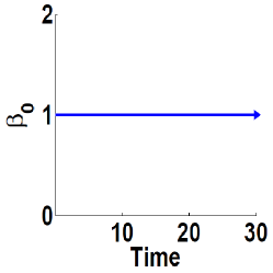
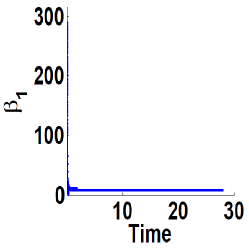
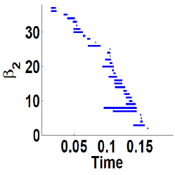
Figure 11: The evolution of the topological invariants of the beta barrel under the Laplace-Beltrami flow.

The above results demonstrate that the proposed Laplace-Beltrami flow based persistent homology is an efficient tool for analyzing the topological structures of protein molecules.

VI.B Fullerene total curvature energy prediction

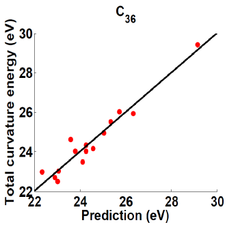
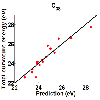
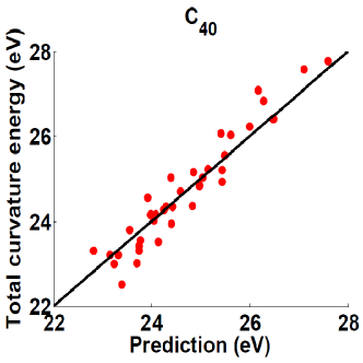
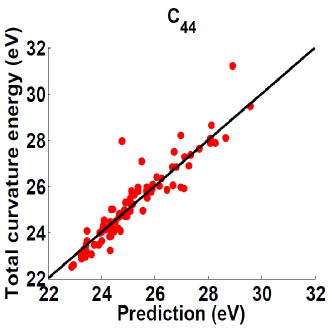
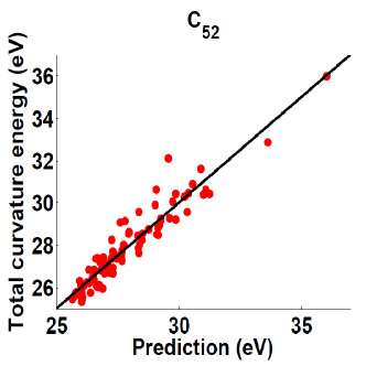
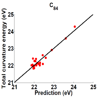
Figure 12: The comparison of fullerene isomer total curvature energies and persistent homology theory predictions.

Having demonstrated the utility of the proposed Laplace-Beltrami flow based persistent homology method for protein characterization, we are interested in the further application of this topological tool for quantitative analysis of carbon fullerene molecules. In particular, we explore the application of the present persistent homology method to the prediction of the total curvature energies of the carbon fullerene isomers. Fullerene molecules admit a large number of isomers, especially when the number of atoms is large. Different isomers with the same chemical formula have different geometric structures which leads to the variations in their total curvature energies. The stability of each given fullerene isomer is determined by its total curvature energy. In general, the higher energy isomer is less stable.

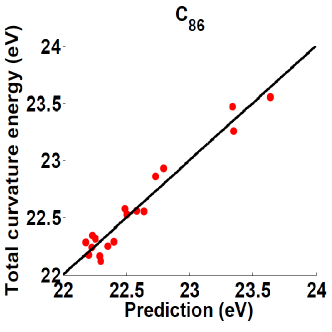
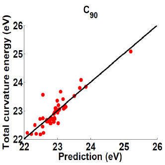
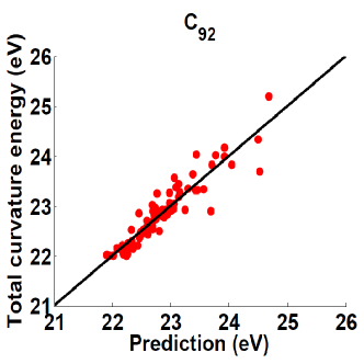
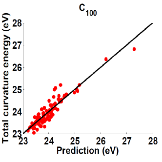
Figure 13: The comparison of fullerene isomer total curvature energies and persistent homology theory predictions (cont’d).

Table 4: The correlation coefficients and standard deviations of the predicted values with respect to total curvature energy data.

Fullerene molecule	Correlation coefficient	Standard deviation
C36	0.9668	0.4345
C38	0.9280	0.5263
C40	0.9665	0.4394
C44	0.9485	0.6211
C52	0.9477	0.5721
C84	0.9389	0.1932
C86	0.9737	0.0998
C90	0.8956	0.2469
C92	0.9326	0.2253
C100	0.9253	0.2364

We assume that different isomers of a fullerene molecule have the same surface area. This assumption is reasonable because all isomers share the same set of atoms and bonds. However, these isomers may have different enclosed volumes as some isomers are more spherical than others. Those isomers that deviate from the spherical shape must have high curvature energies. The more deviation from the sphericity in the structure, the higher curvature energy an isomer has. Additionally, by the iso-perimetric inequality we know that for a class of isomers of a given surface area, the volume is maximized when the isomer is a perfect sphere. For fullerene isomers, more deviation from the sphericity in the structure, the earlier in the time evolution the $\beta_{2}$ bar dies, which leads to a shorter $\beta_{2}$ bar length. Therefore, we can establish a relationship between the persistence of $\beta_{2}$ invariant and the total curvature energy of a fullerene isomer.

In this work, the persistence or bar length of Betti 2, which essentially measures the size of the central cavity, is employed to predict the total curvature energy of carbon fullerene isomers. The Laplace-Beltrami flow is discretized with time stepping size $0.001$ and grid spacing size $0.25$. To quantitatively verify our prediction, the least squares method is employed to fit our predictions of the total curvature energies with the values provided in the web mentioned above. The accuracy of our prediction is evaluated by the correlation coefficient (cc)

$${\rm cc}=\frac{\sum_{i=1}^{N}(L_{i}-\bar{L})(E_{i}-\bar{E})}{[\sum_{i=1}^{N}(L_{i}-\bar{L})^{2}(E_{i}-\bar{E})^{2}]^{1/2}},$$ (25)

where $L_{i}$ represents the bar length of $\beta_{2}$ generated by the Laplace-Beltrami flow based persistent homology method for the $i$th fullerene isomer of a given carbon fullerene family, $\bar{L}$ is the average of the bar length of $\beta_{2}$ over all the isomers of the fullerene, $E_{i}$ is the total curvature energy of the $i$th fullerene isomer, $\bar{E}$ is the average of the total curvature energy over all the isomers of the fullerene. Note that we only count the $\beta_{2}$ bar that is due to the central cavity.

We consider a total of ten different fullerene families with more than 500 fullerene isomers in this study, where the data are chosen from the following rules:

• For a specific carbon fullerene family, if it has less than or equal to 100 isomers, all the data are utilized.

• For a given carbon fullerene family, if there are more than 100 isomers, the first 100 isomer molecules listed in the web are utilized.

Table 5: Total curvature energies of C₃₆ isomers vs lengths of the $\beta_{2}$ bar ($L(\beta_{2})$) obtained with different time stepping sizes.

Total curvature energy (eV)	$L(\beta_{2})$ ($\Delta t=0.0001$)	$L(\beta_{2})$ ($\Delta t=0.0002$)	$L(\beta_{2})$ ($\Delta t=0.0004$)	$L(\beta_{2})$ ($\Delta t=0.0008$)
22.493	6.435	6.436	6.436	6.440
22.688	6.464	6.464	6.464	6.464
22.965	6.601	6.602	6.600	6.608
23.027	6.422	6.422	6.424	6.432
23.469	6.159	6.560	6.164	6.160
24.025	6.240	6.240	6.240	6.248
24.031	6.122	6.124	6.124	6.128
24.152	6.044	6.044	6.048	6.056
24.335	6.122	6.124	6.124	6.128
24.620	6.292	6.292	6.296	6.304
24.938	5.928	5.930	5.928	5.936
25.514	5.852	5.852	5.856	5.856
25.937	5.608	5.606	5.608	5.608
26.013	5.760	5.760	5.760	5.760
29.424	4.901	4.902	4.904	4.904
Correlation coefficient	0.9668	0.9643	0.9669	0.9659
Standard deviation	0.4345	0.4499	0.4339	0.4401

The predicted results and the corresponding total curvature energies are illustrated in Figs. 12 and 13. Table 4 gives the correlation coefficients and standard deviations of the predicted total curvature energies based on the proposed persistent homology theory and the total curvature energy data. Our results for ten different fullerene molecules show good predictions of our differential geometry based persistent homology model.

Table 6: Total curvature energies of C₃₆ isomers vs lengths of the $\beta_{2}$ bar $(L(\beta_{2}))$ obtained with different spatial spacing sizes

Total curvature energy (eV)	$L(\beta_{2})$ ($h=0.15$)	$L(\beta_{2})$ ($h=0.20$)	$L(\beta_{2})$ ($h=0.25$)	$L(\beta_{2})$ ($h=0.30$)
22.493	6.837	6.704	6.435	6.178
22.688	6.845	6.729	6.464	6.410
22.965	6.771	6.621	6.601	6.149
23.027	6.728	6.541	6.422	6.283
23.469	6.638	6.441	6.159	6.002
24.025	6.564	6.440	6.240	5.986
24.031	6.363	6.039	6.122	5.751
24.152	6.359	6.345	6.044	5.762
24.335	6.363	6.309	6.122	5.751
24.620	6.621	6.459	6.292	5.926
24.938	6.291	6.067	5.928	5.723
25.514	6.260	6.048	5.852	5.740
25.937	6.042	5.936	5.608	5.515
26.013	6.087	5.822	5.760	5.626
29.424	5.385	5.186	4.901	4.918
Correlation coefficient	0.9715	0.9804	0.9668	0.9501
Standard deviation	0.4030	0.3349	0.4345	0.5300

To test the reliability and robustness of our method in the isomer total curvature energy prediction, we have carried out our analysis with different grid spacing sizes and time stepping sizes for 15 C₃₆ isomers. Table 5 lists the lengths of $\beta_{2}$ bars obtained with different time stepping sizes ($\Delta t$) and the total curvature energies of C₃₆ isomers. A uniform spatial spacing size of $h=0.25$ is used in this test. Similarly, Table 6 gives the lengths of $\beta_{2}$ bars computed with different grid spacing sizes $h$ and the total curvature energies of C₃₆ isomers. A given time stepping size of $\Delta t=0.0001$ is adopted in this validation. Again, we see a good consistence among our results.

Based on the above spatial and temporal convergent analysis, it is clear that our results are robust and reliable. Therefore, the persistence of Betti 2 has a strong correlation with the total curvature energies of fullerene isomers. These results demonstrate that the persistence of Betti 2 is indeed reversely proportional to the total curvature energies of fullerene isomers. Additionally, the proposed Laplace-Beltrami flow based persistent homology approach performs extremely well in quantitative prediction of topology-function relationship for fullerene isomers.

VII Conclusion

It is well known that topology typically does not distinguish a doughnut and a mug, which implies there is too much reduction in the geometric information. Indeed, topology is seldom used for quantitative description and modeling. In contrast, geometry gives rise to very detailed models for the physical world. At nano scale and/or atomic scale, geometry based models often involve too many degrees of freedom such that their simulations become intractable for many real world problems. Persistent homology is a new branch of algebraic topology that has recently become quite popular for topological simplifications in scientific and engineering applications. Its essential idea is to embed topological invariants in a minimal amount of geometric variation, i.e., a filtration parameter. As a result, persistent homology bridges the traditional topology and geometry.

In the past, most successful applications of persistent homology have been limited to characterization, identification and analysis (CIA) in the literature. Indeed, persistent homology has been rarely employed for quantitative prediction. In our recent work [85], we have introduced molecular topological fingerprints, which treat all barcodes in an equal footing for data CIA. We have also proposed topology-function relationships, which utilize persistent homology as an efficient tool for the physical modeling and quantitative prediction of biomoelcular systems.

In this work, a general procedure is introduced to construct objective-oriented persistent homology approaches for the detection, extraction and/or enhancement of desirable topological traits in data. Our essential idea is to define an objective functional to optimize desirable properties. The optimization leads to a set of operators whose actions enforce the objective functional and give rise to a multiscale representation of the original data. When such a multiscale representation is utilized for filtration, the resulting objective-oriented persistent homology automatically detect, extract and/or amplify the corresponding topological persistence of the data. As a proof of principle, we use the differential geometry theory of surfaces to construct a surface energy functional. The optimization of this functional leads to the Laplace-Beltrami operator, which is able to provide a geometry-embedded filtration of the data of interest. The resulting persistent homology enhances the corresponding geometric structure in topological persistence. The proposed method is intensively validated using benchmark tests and structures with known topological properties.

The application of the proposed geometric flow based topological method is considered to both the CIA and quantitative modeling of proteins and carbon fullerene molecules. We first employ the present method for the analysis of a beta barrel protein. The structure of the beta barrel has a large ring. Topologically, it is interesting to observe a long-lived Betti-1 bar during the time evolution of the Laplace-Beltrami flow.

Another application of the proposed method is the total curvature energy prediction of fullerene isomers. We propose a model to correlate isomer total curvature energy and its structural sphericity. The latter is measured by the length of the Betti 2 bar of the isomer central cavity. Essentially, a more distorted isomer has a higher total curvature energy and a shorter period of persistence of the central cavity Betti 2 bar. In our quantitative energy prediction, we have utilized a total of ten sets of fullerene isomers. Our results indicate that both the proposed Laplace-Beltrami flow based persistent homology method and the present quantitative model work extremely well. All the correlation coefficients are very high.

The present differential geometry based persistent homology opens a new approach for the topological simplification of big data. We expect that other objective functionals can be designed and corresponding objective-oriented persistent homology methods can be developed for specific purposes in data sciences. This approach will also lead to the construction of new objective-oriented partial differential equations (PDEs), geometric PDEs and topological PDEs in the future.

As stated above, all fullerene data are downloaded from a web page: fullerene-isomers. However, it is well known that a web page may not exist after certain time. We therefore present fullerene isomers and their total curvature energies used in the present work in the following tables. The corresponding structure data are available up on request.

Table 7: Fullerene C36 isomers and total curvature energies

Name	Energy (eV)	Name	Energy (eV)	Name	Energy (eV)	Name	Energy (eV)
C36(C2)1	25.937	C36(D2)2	29.424	C36(C1)3	24.938	C36(Cs)4	25.524
C36(D2)5	26.013	C36(D2d)6	24.335	C36(C1)7	24.031	C36(Cs)8	24.025
C36(C2v)9	22.965	C36(C2)10	24.152	C36(C2)11	23.469	C36(C2)12	23.027
C36(D3h)13	24.620	C36(D2d)14	22.493	C36(D6h)15	22.688

Table 8: Fullerene C38 isomers and total curvature energies

Name	Energy (eV)	Name	Energy (eV)	Name	Energy (eV)	Name	Energy (eV)
C38(C2)1	26.613	C38(D3h)2	27.745	C38(C1)3	25.120	C38(C1)4	26.564
C38(C1)5	24.288	C38(C2)6	25.564	C38(C1)7	25.520	C38(C1)8	24.184
C38(D3)9	25.843	C38(C2)10	23.853	C38(C1)11	24.185	C38(C2v)12	24.665
C38(C2)13	23.440	C38(C1)14	23.111	C38(C2v)15	24.069	C38(C3v)16	22.610
C38(C2)17	22.603

Table 9: Fullerene C40 isomers and total curvature energies

Name	Energy (eV)	Name	Energy (eV)	Name	Energy (eV)	Name	Energy (eV)
C40(D5d)1	30.194	C40(C2)2	27.771	C40(D2)3	29.686	C40(C1)4	26.838
C40(Cs)5	26.233	C40(C1)6	27.587	C40(C1)7	27.587	C40(C2v)8	26.421
C40(C2)9	24.856	C40(C1)10	24.933	C40(C2)11	27.092	C40(C1)12	25.038
C40(Cs)13	24.830	C40(Cs)14	24.165	C40(Cs)15	24.343	C40(C2)16	25.035
C40(C1)17	24.549	C40(C2)18	26.062	C40(C2)19	25.165	C40(C3v)20	24.271
C40(C2)21	24.356	C40(C1)22	24.031	C40(C2)23	25.232	C40(Cs)24	23.522
C40(C2)25	24.377	C40(C1)26	23.301	C40(C2)27	23.805	C40(Cs)28	24.700
C40(C2)29	23.416	C40(C3)30	24.163	C40(Cs)31	23.205	C40(D2)32	25.212
C40(D2h)33	26.042	C40(C1)34	23.946	C40(C2)35	23.560	C40(C2)36	22.994
C40(C2v)37	23.015	C40(D2)38	22.522	C40(D5d)39	23.206	C40(Td)40	23.300

Table 10: Fullerene C44 isomers and total curvature energies

Name	Energy (eV)	Name	Energy (eV)	Name	Energy (eV)	Name	Energy (eV)
C44(C2)1	29.456	C44(D2)2	32.322	C44(D3d)3	31.727	C44(C2)4	28.076
C44(C2)5	27.881	C44(C2)6	28.085	C44(C1)7	27.359	C44(C1)8	26.901
C44(C1)9	28.635	C44(C1)10	27.949	C44(Cs)11	27.882	C44(C2)12	27.618
C44(C2v)13	26.848	C44(C2)14	27.270	C44(C1)15	26.036	C44(C1)16	26.020
C44(C1)17	27.492	C44(C1)18	25.806	C44(C1)19	25.968	C44(C2)20	26.256
C44(C1)21	26.389	C44(C1)22	24.685	C44(C1)23	25.012	C44(D2)24	25.872
C44(C1)25	25.218	C44(C1)26	25.950	C44(C1)27	25.505	C44(Cs)28	24.845
C44(C1)29	24.164	C44(C1)30	24.487	C44(C1)31	25.802	C44(C2)32	24.446
C44(Cs)33	25.314	C44(C2)34	27.070	C44(D3)35	31.214	C44(C2)36	24.669
C44(D3h)37	25.905	C44(D3d)38	25.964	C44(C2v)39	24.944	C44(C1)40	24.708
C44(C1)41	25.793	C44(C1)42	24.935	C44(C1)43	25.754	C44(C2)44	25.488
C44(C2)45	25.834	C44(C2)46	26.079	C44(C1)47	24.285	C44(C1)48	25.210
C44(C2)49	24.380	C44(C1)50	24.960	C44(C1)51	24.174	C44(C1)52	23.454
C44(Cs)53	25.790	C44(Cs)54	24.117	C44(C2v)55	23.983	C44(C1)56	24.320
C44(C1)57	23.831	C44(C1)58	24.991	C44(C1)59	23.427	C44(C1)60	24.054
C44(C2)61	24.844	C44(C1)62	24.170	C44(C1)63	24.061	C44(C1)64	24.537
C44(C1)65	24.804	C44(C2)66	26.402	C44(C1)67	23.276	C44(C2)68	23.218
C44(C1)69	22.958	C44(Cs)70	23.619	C44(Cs)71	24.168	C44(D3h)72	22.846
C44(T)73	24.076	C44(C2)74	23.621	C44(D2)75	22.582	C44(C2)76	23.848
C44(C1)77	22.900	C44(C1)78	23.065	C44(C2)79	23.463	C44(D3)80	23.159
C44(C2)81	24.389	C44(S4)82	23.258	C44(D2)83	23.903	C44(Cs)84	24.040
C44(D2)85	25.617	C44(D3d)86	28.214	C44(C2)87	23.220	C44(C1)88	23.049
C44(D2)89	22.513

Table 11: Fullerene C52 isomers and total curvature energies

Name	Energy (eV)	Name	Energy (eV)	Name	Energy (eV)	Name	Energy (eV)
C52(C2)1	32.862	C52(D2)2	35.990	C52(Cs)3	30.452	C52(C1)4	30.393
C52(C2)5	30.646	C52(Cs)6	29.299	C52(C1)7	29.177	C52(C1)8	28.759
C52(C1)9	30.445	C52(C1)10	29.177	C52(C1)11	28.855	C52(C1)12	29.210
C52(C1)13	30.490	C52(C1)14	30.907	C52(C2)15	31.612	C52(C1)16	29.602
C52(C1)17	31.948	C52(C1)18	29.269	C52(C1)19	28.916	C52(C1)20	29.258
C52(C2)21	29.903	C52(C2)22	28.553	C52(C1)23	27.864	C52(C1)24	27.635
C52(C1)25	28.527	C52(C1)26	28.045	C52(C1)27	28.271	C52(C1)28	28.514
C52(C2)29	28.955	C52(C1)30	28.527	C52(C2)31	30.073	C52(C1)32	30.317
C52(C1)33	28.577	C52(C1)34	27.383	C52(C1)35	26.944	C52(C1)36	29.248
C52(C1)37	27.645	C52(Cs)38	29.592	C52(C1)39	27.276	C52(Cs)40	26.724
C52(C1)41	27.721	C52(C1)42	27.676	C52(C2)43	26.717	C52(Cs)44	27.455
C52(C1)45	30.622	C52(C1)46	27.524	C52(C1)47	28.032	C52(C1)48	27.408
C52(C1)49	27.529	C52(C2)50	28.618	C52(C1)51	27.005	C52(C1)52	27.127
C52(C1)53	26.929	C52(C1)54	26.754	C52(C1)55	26.705	C52(C1)56	26.846
C52(C1)57	26.919	C52(D2)58	32.111	C52(C1)59	28.477	C52(C1)60	23.375
C52(C1)61	29.172	C52(C1)62	25.762	C52(C1)63	26.041	C52(C1)64	27.762
C52(C1)65	26.077	C52(Cs)66	25.729	C52(Cs)67	27.443	C52(C1)68	26.383
C52(C1)69	27.389	C52(C1)70	25.753	C52(C1)71	27.405	C52(C1)72	26.846
C52(C1)73	26.857	C52(C1)74	25.468	C52(C1)75	26.336	C52(C1)76	27.267
C52(C1)77	29.103	C52(C1)78	25.652	C52(C1)79	27.349	C52(C1)80	25.765
C52(C1)81	26.857	C52(C2)82	26.813	C52(C2)83	28.263	C52(C2)84	25.361
C52(C1)85	27.436	C52(C1)86	25.508	C52(C1)87	27.288	C52(C2)88	27.449
C52(C1)89	25.532	C52(C1)90	26.098	C52(C1)91	26.693	C52(Cs)92	25.805
C52(C1)93	26.103	C52(D2d)94	26.864	C52(Cs)95	25.937	C52(C1)96	26.124
C52(C1)97	26.130	C52(C1)98	25.646	C52(C2)99	27.367	C52(C1)100	26.255

Table 12: Fullerene C84 isomers and total curvature energies

Name	Energy (eV)	Name	Energy (eV)	Name	Energy (eV)	Name	Energy (eV)
C84(D2)1	24.281	C84(C2)2	23.593	C84(Cs)3	22.389	C84(D2d)4	22.607
C84(D2)5	22.910	C84(C2v)6	22.408	C84(C2v)7	22.270	C84(C2)8	22.167
C84(C2)9	22.124	C84(Cs)10	22.043	C84(C2)11	22.088	C84(C1)12	22.011
C84(C2)13	22.109	C84(Cs)14	22.250	C84(Cs)15	22.012	C84(Cs)16	22.019
C84(C2v)17	22.124	C84(C2v)18	22.159	C84(D3d)19	22.090	C84(Td)20	22.453
C84(D2)21	21.950	C84(D2)22	21.854	C84(D2d)23	21.829	C84(D6h)24	21.990

Table 13: Fullerene C86 isomers and total curvature energies

Name	Energy (eV)	Name	Energy (eV)	Name	Energy (eV)	Name	Energy (eV)
C86(C1)1	23.258	C86(C2)2	23.553	C86(C2)3	23.473	C86(C2)4	22.862
C86(c1)5	22.576	C86(C2)6	22.933	C86(C1)7	22.528	C86(Cs)8	22.562
C86(C2v)9	22.556	C86(C2v)10	22.285	C86(C1)11	22.242	C86(C1)12	22.256
C86(C1)13	22.169	C86(C2)14	22.292	C86(Cs)15	22.178	C86(Cs)16	22.348
C86(C2)17	22.211	C86(C3)18	22.320	C86(D3)19	22.123

Table 14: Fullerene C90 isomers and total curvature energies

Name	Energy (eV)	Name	Energy (eV)	Name	Energy (eV)	Name	Energy (eV)
C90(D5h)1	25.081	C90(C2v)2	24.092	C90(C1)3	23.808	C90(C2)4	23.846
C90(Cs)5	23.521	C90(C2)6	23.080	C90(C1)7	22.894	C90(C2)8	23.407
C90(C1)9	22.716	C90(Cs)10	22.612	C90(C1)11	23.094	C90(C2)12	23.120
C90(C2v)13	23.672	C90(C1)14	23.195	C90(C1)15	23.180	C90(C2v)16	23.355
C90(Cs)17	23.147	C90(C2)18	23.023	C90(C2)19	22.687	C90(C1)20	22.625
C90(C1)21	22.561	C90(C1)22	22.695	C90(C2)23	22.569	C90(C1)24	23.020
C90(C2v)25	23.096	C90(C1)26	22.621	C90(C1)27	22.700	C90(C2)28	22.715
C90(C1)29	22.960	C90(C1)30	22.565	C90(C2)31	22.989	C90(C1)32	22.559
C90(Cs)33	23.060	C90(Cs)34	22.737	C90(Cs)35	22.497	C90(C2v)36	22.939
C90(C2)37	22.748	C90(C1)38	22.614	C90(C2v)39	22.742	C90(C2)40	22.227
C90(C2)41	22.190	C90(C2)42	22.222	C90(C2)43	22.177	C90(C2)44	22.443
C90(C2)45	22.174	C90(C2v)46	22.225

Table 15: Fullerene C92 isomers and total curvature energies

Name	Energy (eV)	Name	Energy (eV)	Name	Energy (eV)	Name	Energy (eV)
C92(D2)1	25.193	C92(C1)2	23.825	C92(C2)3	24.330	C92(C2)4	23.995
C92(Cs)5	23.695	C92(Cs)6	23.638	C92(C2)7	23.316	C92(C1)8	23.051
C92(C2)9	23.351	C92(C1)10	22.769	C92(C1)11	22.837	C92(C1)12	22.888
C92(C1)13	23.188	C92(Cs)14	22.969	C92(Cs)15	22.675	C92(Cs)16	22.913
C92(C2)17	23.831	C92(C1)18	23.325	C92(C2)19	23.336	C92(C1)20	23.448
C92(C2)21	24.031	C92(C2v)22	24.207	C92(C2)23	23.276	C92(Cs)24	22.850
C92(C2)25	23.895	C92(C2)26	23.023	C92(C2)27	23.263	C92(D3)28	23.566
C92(D2h)29	24.174	C92(C1)30	22.941	C92(C2)31	22.878	C92(C1)32	22.733
C92(C1)33	22.922	C92(C2)34	22.706	C92(C2v)35	23.380	C92(C2)36	22.903
C92(C1)37	23.056	C92(C1)38	22.529	C92(C1)39	22.930	C92(C1)40	22.894
C92(C1)41	25.793	C92(C1)42	24.935	C92(C1)43	25.754	C92(C2)92	25.488
C92(C2)45	25.834	C92(C2)46	26.079	C92(C1)47	24.285	C92(C1)48	25.210
C92(C2)49	24.380	C92(C1)50	24.960	C92(C1)51	24.174	C92(C1)52	23.454
C92(Cs)53	25.790	C92(Cs)54	24.117	C92(C2v)55	23.983	C92(C1)56	24.320
C92(C1)57	23.831	C92(C1)58	24.991	C92(C1)59	23.427	C92(C1)60	24.054
C92(C2)61	24.892	C92(C1)62	24.170	C92(C1)63	24.061	C92(C1)64	24.537
C92(C1)65	24.804	C92(C2)66	26.402	C92(C1)67	23.276	C92(C2)68	23.218
C92(C1)69	22.958	C92(Cs)70	23.619	C92(Cs)71	24.168	C92(D3h)72	22.846
C92(T)73	24.076	C92(C2)74	23.621	C92(D2)75	22.582	C92(C2)76	23.848
C92(C1)77	22.900	C92(C1)78	23.065	C92(C2)79	23.463	C92(D3)80	23.159
C92(C2)81	24.389	C92(S4)82	23.258	C92(D2)83	23.903	C92(Cs)84	24.040
C92(D2)85	25.617	C92(D3d)86	28.214

Table 16: Fullerene C100 isomers and total curvature energies

Name	Energy (eV)	Name	Energy (eV)	Name	Energy (eV)	Name	Energy (eV)
C100(C2)1	32.862	C100(D2)2	35.990	C100(Cs)3	30.4100	C100(C1)4	30.393
C100(C2)5	30.646	C100(Cs)6	29.299	C100(C1)7	29.177	C100(C1)8	28.759
C100(C1)9	30.445	C100(C1)10	29.177	C100(C1)11	28.855	C100(C1)12	29.210
C100(C1)13	30.490	C100(C1)14	30.907	C100(C2)15	31.612	C100(C1)16	29.602
C100(C1)17	31.948	C100(C1)18	29.269	C100(C1)19	28.916	C100(C1)20	29.258
C100(C2)21	29.903	C100(C2)22	28.553	C100(C1)23	27.864	C100(C1)24	27.635
C100(C1)25	28.1007	C100(C1)26	28.045	C100(C1)27	28.271	C100(C1)28	28.514
C100(C2)29	28.955	C100(C1)30	28.1007	C100(C2)31	30.073	C100(C1)32	30.317
C100(C1)33	28.577	C100(C1)34	27.383	C100(C1)35	26.944	C100(C1)36	29.248
C100(C1)37	27.645	C100(Cs)38	29.592	C100(C1)39	27.276	C100(Cs)40	26.724
C100(C1)41	27.721	C100(C1)42	27.676	C100(C2)43	26.717	C100(Cs)44	27.455
C100(C1)45	30.622	C100(C1)46	27.1004	C100(C1)47	28.032	C100(C1)48	27.408
C100(C1)49	27.1009	C100(C2)50	28.618	C100(C1)51	27.005	C100(C1)52	27.127
C100(C1)53	26.929	C100(C1)54	26.754	C100(C1)55	26.705	C100(C1)56	26.846
C100(C1)57	26.919	C100(D2)58	32.111	C100(C1)59	28.477	C100(C1)60	23.375
C100(C1)61	29.172	C100(C1)62	25.762	C100(C1)63	26.041	C100(C1)64	27.762
C100(C1)65	26.077	C100(Cs)66	25.729	C100(Cs)67	27.443	C100(C1)68	26.383
C100(C1)69	27.389	C100(C1)70	25.753	C100(C1)71	27.405	C100(C1)72	26.846
C100(C1)73	26.857	C100(C1)74	25.468	C100(C1)75	26.336	C100(C1)76	27.267
C100(C1)77	29.103	C100(C1)78	25.6100	C100(C1)79	27.349	C100(C1)80	25.765
C100(C1)81	26.857	C100(C2)82	26.813	C100(C2)83	28.263	C100(C2)84	25.361
C100(C1)85	27.436	C100(C1)86	25.508	C100(C1)87	27.288	C100(C2)88	27.449
C100(C1)89	25.532	C100(C1)90	26.098	C100(C1)91	26.693	C100(Cs)92	25.805
C100(C1)93	26.103	C100(D2d)94	26.864	C100(Cs)95	25.937	C100(C1)96	26.124
C100(C1)97	26.130	C100(C1)98	25.646	C100(C2)99	27.367	C100(C1)100	26.255

References

- [1] P. W. Bates, Z. Chen, Y. H. Sun, G. W. Wei, and S. Zhao. Geometric and potential driving formation and evolution of biomolecular surfaces. J. Math. Biol., 59:193–231, 2009.
- [2] P. W. Bates, G. W. Wei, and S. Zhao. The minimal molecular surface. arXiv:q-bio/0610038v1, [q-bio.BM], 2006.
- [3] P. W. Bates, G. W. Wei, and S. Zhao. The minimal molecular surface. Midwest Quantitative Biology Conference, Mission Point Resort, Mackinac Island, MI:September 29 – October 1, 2006.
- [4] P. W. Bates, G. W. Wei, and Shan Zhao. Minimal molecular surfaces and their applications. Journal of Computational Chemistry, 29(3):380–91, 2008.
- [5] Paul Bendich, Herbert Edelsbrunner, and Michael Kerber. Computing robustness and persistence for images. IEEE Transactions on Visualization and Computer Graphics, 16:1251–1260, 2010.
- [6] P. Blomgren and T.F. Chan. Color TV: total variation methods for restoration of vector-valued images. Image Processing, IEEE Transactions on, 7(3):304–309, 1998.
- [7] Peter Bubenik and Peter T. Kim. A statistical approach to persistent homology. Homology, Homotopy and Applications, 19:337–362, 2007.
- [8] G. Carlsson. Topology and data. Am. Math. Soc, 46(2):255–308, 2009.
- [9] G. Carlsson, T. Ishkhanov, V. Silva, and A. Zomorodian. On the local behavior of spaces of natural images. International Journal of Computer Vision, 76(1):1–12, 2008.
- [10] V. Carstensen, R. Kimmel, and G. Sapiro. Geodesic active contours. International Journal of Computer Vision, 22:61–79, 1997.
- [11] Thomas Cecil. A numerical method for computing minimal surfaces in arbitrary dimension. J. Comput. Phys., 206(2):650–660, 2005.
- [12] H. W. Chang, S. Bacallado, V. S. Pande, and G. E. Carlsson. Persistent topology and metastable state in conformational dynamics. PLos ONE, 8(4):e58699, 2013.
- [13] Duan Chen, Zhan Chen, and G. W. Wei. Quantum dynamics in continuum for proton transport II: Variational solvent-solute interface. International Journal for Numerical Methods in Biomedical Engineering, 28:25 – 51, 2012.
- [14] Duan Chen and G. W. Wei. Quantum dynamics in continuum for proton transport—Generalized correlation. J Chem. Phys., 136:134109, 2012.
- [15] Z. Chen, N. A. Baker, and G. W. Wei. Differential geometry based solvation models I: Eulerian formulation. J. Comput. Phys., 229:8231–8258, 2010.
- [16] Z. Chen, N. A. Baker, and G. W. Wei. Differential geometry based solvation models II: Lagrangian formulation. J. Math. Biol., 63:1139– 1200, 2011.
- [17] Z. Chen and G. W. Wei. Differential geometry based solvation models III: Quantum formulation. J. Chem. Phys., 135:194108, 2011.
- [18] Z. Chen, Shan Zhao, J. Chun, D. G. Thomas, N. A. Baker, P. B. Bates, and G. W. Wei. Variational approach for nonpolar solvation analysis. Journal of Chemical Physics, 137(084101), 2012.
- [19] L. T. Cheng, Joachim Dzubiella, Andrew J. McCammon, and B. Li. Application of the level-set method to the implicit solvation of nonpolar molecules. Journal of Chemical Physics, 127(8), 2007.
- [20] David L. Chopp. Computing minimal surfaces via level set curvature flow. J. Comput. Phys., 106(1):77–91, 1993.
- [21] Y. Dabaghian, F. Memoli, L. Frank, and G. Carlsson. A topological paradigm for hippocampal spatial map formation using persistent homology. PLoS Comput Biol, 8(8):e1002581, 08 2012.
- [22] T. K. Dey, K. Y. Li, J. Sun, and C. S. David. Computing geometry aware handle and tunnel loops in 3d models. ACM Trans. Graph., 27, 2008.
- [23] Tamal K. Dey and Y. S. Wang. Reeb graphs: Approximation and persistence. Discrete and Computational Geometry, 49(1):46–73, 2013.
- [24] Barbara Di Fabio and Claudia Landi. A mayer-vietoris formula for persistent homology with an application to shape recognition in the presence of occlusions. Foundations of Computational Mathematics, 11:499–527, 2011.
- [25] H. Edelsbrunner, D. Letscher, and A. Zomorodian. Topological persistence and simplification. Discrete Comput. Geom., 28:511–533, 2002.
- [26] Herbert Edelsbrunner and John Harer. Computational topology: an introduction. American Mathematical Soc., 2010.
- [27] X. Feng and A. Prohl. Analysis of a fully discrete finite element method for the phase field model and approximation of its sharp interface limits. Mathematics of Computation, 73:541–567, 2004.
- [28] X. Feng, K. L. Xia, Y. Y. Tong, and G. W. Wei. Multiscale geometric modeling of macromolecules II: lagrangian representation. Journal of Computational Chemistry, 34:2100–2120, 2013.
- [29] Patrizio Frosini and Claudia Landi. Size theory as a topological tool for computer vision. Pattern Recognition and Image Analysis, 9(4):596–603, 1999.
- [30] Patrizio Frosini and Claudia Landi. Persistent betti numbers for a noise tolerant shape-based approach to image retrieval. Pattern Recognition Letters, 34:863–872, 2013.
- [31] M. Gameiro, Y. Hiraoka, S. Izumi, M. Kramar, K. Mischaikow, and V. Nanda. Topological measurement of protein compressibility via persistence diagrams. preprint, 2013.
- [32] R. Ghrist. Barcodes: The persistent topology of data. Bull. Amer. Math. Soc., 45:61–75, 2008.
- [33] J. Gomes and O. D. Faugeras. Using the vector distance functions to evolve manifolds of arbitrary codimension. Lecture Notes in Computer Science, 2106:1–13, 2001.
- [34] J. B. Greer and A. L. Bertozzi. H-1 solutions of a class of fourth order nonlinear equations for image processing. Discrete and Continuous Dynamical Systems, 10:349–366, 2004.
- [35] J. B. Greer and A. L. Bertozzi. Traveling wave solutions of fourth order pdes for image processingl. SIAM Journal on Mathematics Analysis, 36:38–68, 2004.
- [36] J. Guan, Z. Q. Jin, Z. Zhu, and D. Tománek. Local curvature and stability of two-dimensional systems. preprint, 2014.
- [37] Shaun Harker, Konstantin Mischaikow, Marian Mrozek, Vidit N, Hubert Wagner, and Mateusz Juda. The efficiency of a homology algorithm based on discrete morse theory and coreductions. Proceeding of the 3rd International Workshop on Computational Topology in Image Context, Image A, pages 41–47, 2010.
- [38] Shaun Harker, Konstantin Mischaikow, Marian Mrozek, and Vidit Nanda. Discrete Morse theoretic algorithms for computing homology of complexes and maps. Found. Comput. Math., pages doi:10.1007/s10208–013–9145–0, 2013.
- [39] Allen Hatcher. Algebraic Topology. Cambridge University Press, 2001.
- [40] D. Horak, S Maletic, and M. Rajkovic. Persistent homology of complex networks. Journal of Statistical Mechanics: Theory and Experiment, 2009(03):P03034, 2009.
- [41] Z. M. Jin and X. P. Yang. Strong solutions for the generalized perona-malik equation for image restoration. Nonlinear Analysis-Theory Methods and Applications, 73:1077–1084, 2010.
- [42] T. Kaczynski, K. Mischaikow, and M. Mrozek. Computational homology. Springer-Verlag, 2004.
- [43] P. M. Kasson, A. Zomorodian, S. Park, N. Singhal, L. J. Guibas, and V. S. Pande. Persistent voids a new structural metric for membrane fusion. Bioinformatics, 23:1753–1759, 2007.
- [44] Bala Krishnamoorthy, Scott Provan, and Alexander Tropsha. A topological characterization of protein structure. In Data Mining in Biomedicine, Springer Optimization and Its Applications, pages 431–455, 2007.
- [45] H Lee, H. Kang, M. K. Chung, B. Kim, and D. S. Lee. Persistent brain network homology from the perspective of dendrogram. Medical Imaging, IEEE Transactions on, 31(12):2267–2277, Dec 2012.
- [46] Y. Li and F. Santosa. A computational algorithm for minimizing total variation in image restoration. IEEE Transactions on Image Processing, 5(6):987–95, 1996.
- [47] Xu Liu, Zheng Xie, and Dongyun Yi. A fast algorithm for constructing topological structure in large data. Homology, Homotopy and Applications, 14:221–238, 2012.
- [48] Karol Mikula and Daniel Sevcovic. A direct method for solving an anisotropic mean curvature flow of plane curves with an external force. Mathematical Methods in the Applied Sciences, 27(13):1545–1565, 2004.
- [49] K. Mischaikow, M Mrozek, J. Reiss, and A. Szymczak. Construction of symbolic dynamics from experimental time series. Physical Review Letters, 82:1144–1147, 1999.
- [50] K. Mischaikow and V. Nanda. Morse theory for filtrations and efficient computation of persistent homology. Discrete and Computational Geometry, 50(2):330–353, 2013.
- [51] David Mumford and Jayant Shah. Optimal approximations by piecewise smooth functions and associated variational problems. Communications on Pure and Applied Mathematics, 42(5):577–685, 1989.
- [52] Vidit Nanda. Perseus: the persistent homology software. Software available at http://www.sas.upenn.edu/~vnanda/perseus.
- [53] P. Niyogi, S. Smale, and S. Weinberger. A topological view of unsupervised learning from noisy data. SIAM Journal on Computing, 40:646–663, 2011.
- [54] K. Opron, K. L. Xia, and G. W. Wei. Fast and anisotropic flexibility-rigidity index for protein flexibility and fluctuation analysis. Journal of Chemical Physics, 140:234105, 2014.
- [55] S. Osher and J.A. Sethian. Fronts propagating with curvature-dependent speed: algorithms based on Hamilton-Jacobi formulations. Journal of computational physics, 79(1):12–49, 1988.
- [56] Stanley Osher and Ronald P. Fedkiw. Level set methods: An overview and some recent results. J. Comput. Phys., 169(2):463–502, 2001.
- [57] Stanley Osher and Leonid I. Rudin. Feature-oriented image enhancement using shock filters. SIAM Journal on Numerical Analysis, 27(4):919–940, 1990.
- [58] D. Pachauri, C. Hinrichs, M.K. Chung, S.C. Johnson, and V. Singh. Topology-based kernels with application to inference problems in alzheimer’s disease. Medical Imaging, IEEE Transactions on, 30(10):1760–1770, Oct 2011.
- [59] J. K. Park and G. W. Wei. A molecular level prototype for mechanoelectrical transducers in mammalian hair cells. Journal of Computational Neuroscience, 35:231–241, 2014.
- [60] Bastian Rieck, Hubert Mara, and Heike Leitte. Multivariate data analysis using persistence-based filtering and topological signatures. IEEE Transactions on Visualization and Computer Graphics, 18:2382–2391, 2012.
- [61] Vanessa Robins. Towards computing homology from finite approximations. In Topology Proceedings, volume 24, pages 503–532, 1999.
- [62] Leonid I. Rudin, Stanley Osher, and Emad Fatemi. Nonlinear total variation based noise removal algorithms. In Proceedings of the eleventh annual international conference of the Center for Nonlinear Studies on Experimental mathematics : computational issues in nonlinear science, pages 259–268, Amsterdam, The Netherlands, The Netherlands, 1992. Elsevier North-Holland, Inc.
- [63] G. Sapiro and D. L. Ringach. Anisotropic diffusion of multivalued images with applications to color filtering. Image Processing, IEEE Transactions on, 5(11):1582–1586, 1996.
- [64] A. Sarti, R. Malladi, and J. A. Sethian. Subjective surfaces: A geometric model for boundary completion. International Journal of Computer Vision, 46(3):201–221, 2002.
- [65] J. A. Sethian. Evolution, implementation, and application of level set and fast marching methods for advancing fronts. J. Comput. Phys., 169(2):503–555, 2001.
- [66] V. D. Silva and R Ghrist. Blind swarms for coverage in 2-d. In In Proceedings of Robotics: Science and Systems, page 01, 2005.
- [67] G. Singh, F. Memoli, T. Ishkhanov, G. Sapiro, G. Carlsson, and D. L. Ringach. Topological analysis of population activity in visual cortex. Journal of Vision, 8(8), 2008.
- [68] Peter Smereka. Semi-implicit level set methods for curvature and surface diffusion motion. Journal of Scientific Computing, 19(1):439–456, 2003.
- [69] N. Sochen, R. Kimmel, and R. Malladi. A general framework for low level vision. Image Processing, IEEE Transactions on, 7(3):310–318, 1998.
- [70] D. Strombom. Persistent Homology in the cubical setting. Master’s Thesis, Lulea University of Technology, 2007.
- [71] Andrew Tausz, Mikael Vejdemo-Johansson, and Henry Adams. Javaplex: A research software package for persistent (co)homology. Software available at http://code.google.com/p/javaplex, 2011.
- [72] C. Wagner, C. Chen, and E. Vucini. Efficient computation of persistent homology for cubical data. Topological Methods in Data Analysis and Visualization II, page Springer Heidelberg Dordrecht London New York, 2012.
- [73] Bei Wang, Brian Summa, Valerio Pascucci, and M. Vejdemo-Johansson. Branching and circular features in high dimensional data. IEEE Transactions on Visualization and Computer Graphics, 17:1902–1911, 2011.
- [74] Y. Wang, G. W. Wei, and Si-Yang Yang. Partial differential equation transform – Variational formulation and Fourier analysis. International Journal for Numerical Methods in Biomedical Engineering, 27:1996–2020, 2011.
- [75] Y. Wang, G. W. Wei, and Si-Yang Yang. Mode decomposition evolution equations. Journal of Scientific Computing, 50:495–518, 2012.
- [76] Y. Wang, G. W. Wei, and Si-Yang Yang. Selective extraction of entangled textures via adaptive pde transform. International Journal in Biomedical Imaging, 2012:Article ID 958142, 2012.
- [77] G. W. Wei. Generalized Perona-Malik equation for image restoration. IEEE Signal Processing Lett., 6:165–167, 1999.
- [78] G. W. Wei. Differential geometry based multiscale models. Bulletin of Mathematical Biology, 72:1562 – 1622, 2010.
- [79] G. W. Wei and Y. Q. Jia. Synchronization-based image edge detection. Europhysics Letters, 59(6):814–819, 2002.
- [80] G. W. Wei, Y. H. Sun, Y. C. Zhou, and M. Feig. Molecular multiresolution surfaces. arXiv:math-ph/0511001v1, pages 1 – 11, 2005.
- [81] Guo-Wei Wei. Multiscale, multiphysics and multidomain models I: Basic theory. Journal of Theoretical and Computational Chemistry, 12(8):1341006, 2013.
- [82] Guo-Wei Wei, Qiong Zheng, Zhan Chen, and Kelin Xia. Variational multiscale models for charge transport. SIAM Review, 54(4):699 – 754, 2012.
- [83] T. J. Willmore. Riemannian Geometry. Oxford University Press, USA, 1997.
- [84] K. L. Xia, X. Feng, Y. Y. Tong, and G. W. Wei. Multiscale geometric modeling of macromolecules i: Cartesian representation. Journal of Computational Physics, 275:912–936, 2014.
- [85] K. L. Xia and G. W. Wei. Persistent homology analysis of protein structure, flexibility and folding. International Journal for Numerical Methods in Biomedical Engineerings, 30:814–844, 2014.
- [86] M. Xu and S. L. Zhou. Existence and uniqueness of weak solutions for a fourth-order nonlinear parabolic equation. Journal of Mathematical Analysis and Applications, 325(1):636–654, 2007.
- [87] Y. Yao, J. Sun, X. H. Huang, G. R. Bowman, G. Singh, M. Lesnick, L. J. Guibas, V. S. Pande, and G. Carlsson. Topological methods for exploring low-density states in biomolecular folding pathways. The Journal of Chemical Physics, 130:144115, 2009.
- [88] Z. Y. Yu and C. Bajaj. Computational approaches for automatic structural analysis of large biomolecular complexes. IEEE/ACM Trans Comput Biol Bioinform, 5:568–582, 2008.
- [89] Y. Zhang, G. Xu, and C. Bajaj. Quality meshing of implicit solvation models of biomolecular structures. Computer Aided Geometric Design, 23(6):510–30, 2006.
- [90] Shan Zhao. Pseudo-time-coupled nonlinear models for biomolecular surface representation and solvation analysis. International Journal for Numerical Methods in Biomedical Engineering, 27:1964–1981, 2011.
- [91] Shan Zhao. Operator splitting adi schemes for pseudo-time coupled nonlinear solvation simulations. Journal of Computational Physics, 257:1000 – 1021, 2014.
- [92] Q. Zheng, S. Y. Yang, and G. W. Wei. Molecular surface generation using PDE transform. International Journal for Numerical Methods in Biomedical Engineering, 28:291–316, 2012.
- [93] Qiong Zheng, Duan Chen, and G. W. Wei. Second-order Poisson-Nernst-Planck solver for ion transport. Journal of Comput. Phys., 230:5239 – 5262, 2011.
- [94] Qiong Zheng and G. W. Wei. Poisson-Boltzmann-Nernst-Planck model. Journal of Chemical Physics, 134:194101, 2011.
- [95] A. Zomorodian and G. Carlsson. Computing persistent homology. Discrete Comput. Geom., 33:249–274, 2005.
- [96] Afra Zomorodian and Gunnar Carlsson. Localized homology. Computational Geometry - Theory and Applications, 41(3):126–148, 2008.