Could the Earth's surface Ultraviolet irradiance be blamed for the global warming?(II)
——Ozone layer depth reconstruction via HEWV effect

Abstract

It is suggested by Chen et al. that the Earth's surface Ultraviolet irradiance ($280-400$ nm) could influence the Earth's surface temperature variation by ``Highly Excited Water Vapor" (HEWV) effect. In this manuscript, we reconstruct the developing history of the ozone layer depth variation from 1860 to 2011 based on the HEWV effect. It is shown that the reconstructed ozone layer depth variation correlates with the observational variation from 1958 to 2005 very well ($R=0.8422$, $P>99.9\%$). From this reconstruction, we may limit the spectra band of the surface Ultraviolet irradiance referred in HEWV effect to Ultraviolet B ($280-320$ nm).

I introduction

It is suggested that the surface solar Ultraviolet (UV) irradiance ($280-400$ nm, similarly hereinafter) may have the ability to influence the Earth's surface temperature by ``Highly Excited Water Vapor" (HEWV) effect Chen et al. (2014). Based on the HEWV effect, it is schematically shown in Fig. 1 that the physical way of solar UV irradiance influences the Earth's surface temperature: Part of the UV irradiance emitted by the Sun is absorbed by the Earth's ozone layer and cloud, while the rest reaches to the lower troposphere and influences the surface temperature via HEWV effect. In this manuscript, we suggest a model to obtain the UV irradiance absorbed by ozone layer and the cloud by employing the Earth's surface temperature data and solar UV irradiance data at the top of the Earth's atmosphere. The UV irradiance absorbed by ozone layer and the cloud could describe the variation of ozone layer or cloud.

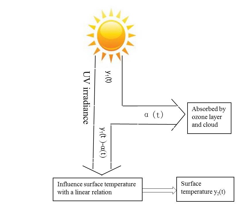
Figure 1: The schematic diagram of physical relation between solar UV irradiance and surface temperature

II the model

In our model, we assume a signal $y_{1}=f_{1}(t)$ goes through a linear system box, which is in a steady state. It is schematically shown in Fig. 2. Then, we can obtain a new signal $y_{2}=f_{2}(t)$, and $y_{1}$ has a linear relation with $y_{2}$, namely

$$y_{1}=Ky_{2}+b.$$ (1)

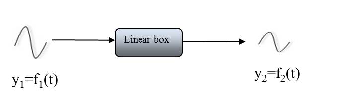
Figure 2: Diagrammatic sketch of the model system. Signal $y_{1}$ changes to $y_{2}$ after getting through the linear system

Based on HEWV effect, we suggest the surface UV irradiance influences the surface temperature linearly. Equation (1) can be employed to describe the relation between surface temperature and surface UV irradiance in spectra band $280-400$ nm. In our model, the Sun emits $y_{1}(t)$ solar UV irradiance in spectra band 280-400 nm to the top of the Earth's atmosphere at the time $t$, and $\alpha(t)$ is absorbed by ozone layer and cloud. The rest part $y_{1}(t)-\alpha(t)$ goes to the lower troposphere and influences the surface temperature $y_{2}(t)$ in a linear relation:

$$y_{1}(t)-\alpha(t)=Ky_{2}(t)+b,$$ (2)

or, it can be rewritten as follow:

$$\alpha(t)=y_{1}(t)-Ky_{2}(t)-b.$$ (3)

The solar UV irradiance data in spectra band $280-400$ nm $y_{1}(t)$ and surface temperature data $y_{2}(t)$ can be obtained. The amounts absorbed by ozone layer and cloud $\alpha(t)$ can be obtained from Eq. (3) for given $K$ and $b$, which can describe the variation of the ozone layer or cloud.

An appropriate way to obtain $K$ and $b$ is to find the years when the ozone layer and cloud did not change (i.e. $\rm\alpha(t)=\alpha_{0}=\rm{constant}$). If this happened, Eq. (2) can be rewritten as

$$y_{1}(t)=Ky_{2}(t)+C,$$ (4)

where $C=b+\alpha_{0}$. Eq. (4) can be employed to obtain the coefficients $K$ and $C$ using the data of $y_{1}$ and $y_{2}$ during these years. Once we know the values of $K$ and $C$, the UV irradiance anomaly absorbed by the ozone layer and the cloud, $\Delta\alpha(t)$, can be obtained as follows

$$\Delta\alpha(t)=y_{1}(t)-Ky_{2}(t)-C,$$ (5)

where $\Delta\alpha(t)=\alpha(t)-\alpha_{0}$. It is clearly that $\rm\Delta\alpha$ can also describe the variation of ozone layer or cloud.

However, we could only find the years when the cloud and ozone layer are keeping the same roughly. This means we could just obtain $\rm\alpha(t)\approx\alpha_{0}$. In this case we can search for the years when the $y_{1}(t)$ correlated with $y_{2}(t)$ well, and employ the linear fitting to obtain the values of $K$ and $C$.

Based on Eq. (5), HEWV effect can be shown via comparing $\Delta\alpha$ with the observed ozone layer depth data or cloud data.

III Data

In this manuscript, the detail data of the surface temperature and solar UV irradiance can be taken from the public data source, they are listed as below:

III.1 Surface temperature (ST)

Global yearly mean surface temperature anomaly from 1860 to 2011 is obtained from HadCRUT3 in Climate Research Unit (CRU) Brohan et al. (2006).

III.2 Solar UV irradiance

Solar Spectra Irradiance (SSI) variation in spectra band $280-400$ nm from 1860 to 2005 is reconstructed by Krivova et al. Krivova et al. (2010).

III.3 Total Solar irradiance (TSI)

Also, the Total Solar Irradiance (TSI) can also be employed to reconstruct $\Delta\alpha$, because the variation of the TSI can describe the property of the SSI in spectra band $280-400$ nm very well. We test the relation between reconstructed SSI and TSI from 1860 to 2005 and find they correlate with each other very well ($R=0.8402$, $P>99.9$%). Moreover, we can obtain satellite observational data after 1979, which could make the value closer to the real TSI variation and may reconstruct the $\Delta\alpha$ more accurate.

The TSI data from 1850 to 1978 was reconstructed by Judith Lean Lean et al. (1995). Satellite data from 1979 to 2003 is from the VIRGO Experiment on the cooperative ESA/NASA Mission SoHO Experiment (2003). Satellite data from 2002 to 2011 is from SORCE TIM Total Solar Irradiance NASA (2013).

III.4 Ozone layer depth

The annual average of global ($65\rm{{}^{o}S}-65\rm{{}^{o}N}$) column total ozone variation from 1958 to 2005 was compiled by Johnston Johnston (2006), which was synthesized the Ground-based observations data and the satellite observations data. The Ground-based observations data from 1958 to 1977 was analyzed by Angell and Korshover in Carbon Dioxide Information Analysis Center (CDIAC) Angell and Korshover (1989). The 1978 to 1992 satellite data was presented by Total Ozone Mapping Spectrometer (TOMS), NASA, measured by Nimbus-7 satellite TOMS (2006a). The ozone layer data from 1993 to 1994 was obtained from Meteor-3 satellite by TOMS, NASA TOMS (2006b). The 1995 data was analyzed by Weber Weber . The ozone layer data from 1996 to 2005 was presented by TOMS TOMS .

IV Results

IV.1 Reconstruct ozone layer depth by employing SSI and ST

Figure 3(A) shows the comparison of ST ($y_{2}$) and SSI ($y_{1}$) variation from 1910 to 1970 in 11-yr moving average. Good correlation is found between them ($R=0.6750$, $P>99.9$%), so we suppose ozone layer or cloud did not change much in this period (we deduct the time series during 1937 and 1945, in the global war II, when there were not enough observational data Kaplan et al. (1998)) and employ them to calculate the parameters $K$ and $C$ using linear fitting method. The linear fitting result is shown in Fig. 3(B). The parameters: $K=3.37\times 10^{6}$ and $C=1.28\times 10^{9}$.

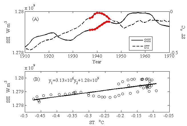
Figure 3: (A) Comparison between Solar spectra irradiance (SSI) in spectra band $280-400$ nm and surface temperature (ST) from 1910 to 1970 (both data are in $11$-yr moving average), data from 1937 to 1945 being deducted (in red color); (B) Linear fit of the two series.

We can use the parameters $K$ and $C$ to calculate the variation of $\rm\Delta\alpha$ based on Eq. (5). The result of $\rm\Delta\alpha$ is shown in Fig. 4. Fig. 4(A) shows the 11-yr moving average variation from 1860 to 2005, compared with observed 11-yr moving average ozone layer depth variation from 1958 to 2005. We find a good correlation between them ($R=0.8965$, $P>99.9$%). Fig. 4(B) shows the yearly variation of $\rm\Delta\alpha$, compared with the yearly ozone layer depth observed variation. Good correlation between them is also found: $R=0.6323$, $P>99.9$%.

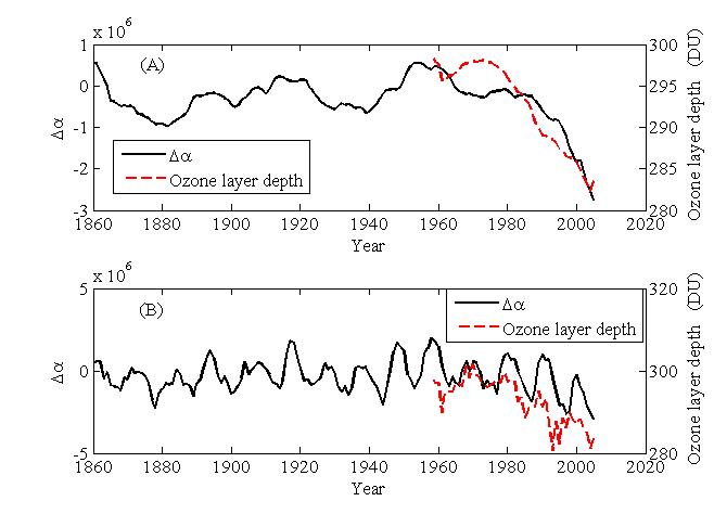
Figure 4: Variation of $\rm\Delta\alpha$ from 1860 to 2005 (by employing SSI). (A): The 11-yr moving average variation of $\rm\Delta\alpha$, compared with the observed 11-yr moving average ozone layer depth variation from 1958 to 2005. (B): Yearly variation of $\rm\Delta\alpha$, compared with the yearly variation of observational ozone layer depth from 1958 to 2005

Based on the good correlation above, we can reconstruct the ozone layer depth variation from 1860 to 2005. Firstly, we fit the linear relation between $\rm\Delta\alpha$ and ozone layer depth by applying $\rm\Delta\alpha$ and observational ozone layer depth data from 1958 to 2005, and it can be written as follows

$$y_{o}=5.83\times 10^{-6}\Delta\alpha+295.99,$$ (6)

where $y_{o}$ is the ozone layer depth. We expand the relation described by Eq. (6) to the whole $\rm\Delta\alpha$ and get the reconstructed ozone layer variation from 1860 to 2005. This is shown in Fig. 5.

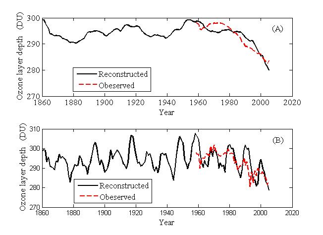
Figure 5: Reconstructed ozone layer depth variation from 1860 to 2005 (by employing SSI data), compared with the observational data. (A): In 11-yr moving average. (B): Yearly variation

IV.2 Reconstruct ozone layer depth by employing TSI and ST

The TSI $(y_{1})$ and ST $(y_{2})$ data from 1910 to 1970 are applied (time series during 1937 and 1945 is deducted) (See Fig. 6(A)). We employ linear fitting and get $K=3.5$ and $C=1366.3$ (See Fig. 6(B)).

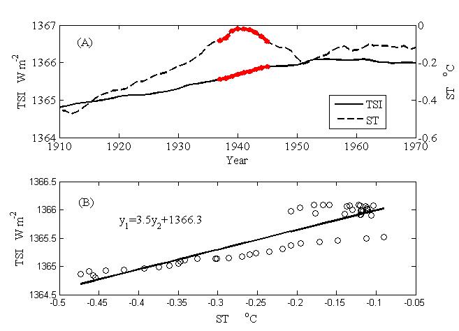
Figure 6: Comparison between Total Solar irradiance (TSI) and surface temperature (ST) from 1910 to 1970, data from 1937 to 1945 being deducted (in red color); (B) Linear fitting of the two series.

$K$ and $C$ are employed to calculate the variation of $\rm\Delta\alpha$ based on Eq.( 5). The result of $\rm\Delta\alpha$ is shown in Fig. 7. Fig. 7(A) shows the 11-yr moving average variation from 1860 to 2011, compared with observed 11-yr moving average ozone layer depth variation from 1958 to 2005. We find a good correlation between them ($R=0.9822$, $P>99.9$%). Fig. 7(B) shows the yearly variation of $\rm\Delta\alpha$, compared with the yearly ozone layer depth observed variation. Good correlation between them is also found ($R=0.8422$, $P>99.9$%). This result of $\rm\Delta\alpha$ is much better than that in SSI occasion.

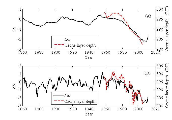
Figure 7: Variation of $\rm\Delta\alpha$ from 1860 to 2011 (by employing TSI). (A): The 11-yr moving average variation of $\rm\Delta\alpha$, compared with the observed 11-yr moving average ozone layer depth variation from 1958 to 2005. (B): Yearly variation of $\rm\Delta\alpha$, compared with the yearly variation of observational ozone layer depth from 1958 to 2005

We could also reconstruct the ozone layer depth variation from 1860 to 2011 based on the linear fitting relation between $\rm\Delta\alpha$ and observed ozone layer depth from 1958 to 2005:

$$y_{o}=6.72\Delta\alpha+297.00.$$ (7)

We expand the relation described by Eq. (7) to the whole $\rm\Delta\alpha$ and get the reconstructed ozone layer variation from 1860 to 2011 as shown in Fig. 8.

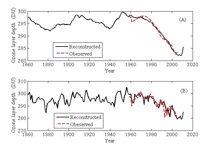
Figure 8: Reconstructed ozone layer variation (using TSI) compared with the observed ozone layer variation. (A): In 11-yr moving average; (B) Yearly variation

V discussion

We could see from Fig. 8 that the reconstructed ozone layer depth data describes the property of the ozone layer depth variation very well, but there are still some differences, such as the opposite variation during 1993 and 2000. The difference may led by the volcano eruption in 1991 and El Niño and La Niño in 1997-1999. Researchers have pointed the cooling effect of the volcanic eruption to the surface temperature, such as Robock and Mao shows that for two years following great volcanic eruptions, the surface of the Earth could be cooled significantly by $0.1\rm{{}^{o}C}\sim 0.2\rm{{}^{o}C}$ in the global mean scale Robock and Mao (1995). In 1991, the volcanic eruption of Mount Pinatubo occurred, cooling the Earth's surface in the following $2$ years, which will lead to a lower value of the reconstructed surface UV irradiance, then a higher UV irradiance absorbed by ozone layer in the reconstruction, and eventually cause a higher reconstructed ozone layer depth near 1993. This suggestion could also interpret the higher reconstructed ozone layer depth data in 1985, when the volcanic eruption in 1983. El Niño could lead a warmer phenomenon in the Earth's surface Robock and Mao (1995). The El Niño appearance in 1997-1998 could lead a warmer surface temperature, which will lead to a lower value of the reconstructed ozone layer depth variation near 1998. We can see the same phenomenon in the year of 1987-1988, when the El Niño occurred.

The signal of the cloud cover doesn't be recognized obviously. Cloud cover is compared with the $\rm\Delta\alpha$ in Fig. 9. The global mean cloud coverage data is obtained from International Satellite cloud climatology Project (ISCCP), NASA ISCCP and NASA . They don't show an apparent correlation ($R=0.4995$, $P>95$%), as obviously as the $\rm\Delta\alpha$ with ozone layer depth ($R=0.8422$, $P>99.9$%). The reason why the cloud cover signal doesn't been recognized obviously need to do more researches. But based on the results, we may suggest that the ozone layer plays more important role in the HEWV effect. The spectra band absorbed by ozone layer is UVB ($280-320$ nm), and this result may limit the spectra that works in HEWV effect to UVB irradiance. More deeper researches should be done before we get a more clear conclusion.

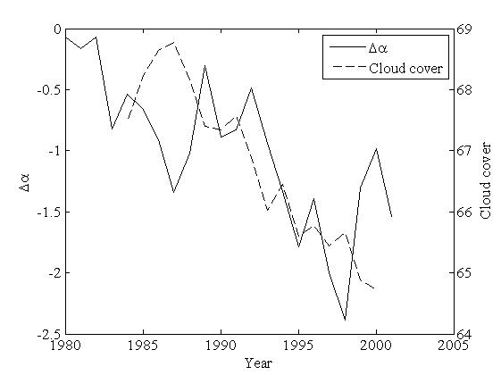
Figure 9: Comparison of the cloud cover variation (Unit: %) and $\rm\Delta\alpha$