On Transitory Queueing Harsha Honnappa EE Department, University of Southern California
honnappa@usc.edu Rahul Jain EE & ISE Departments, University of Southern California
rahul.jain@usc.edu Amy R. Ward Marshall School of Business, University of Southern California
amyward@usc.edu

We introduce a framework and develop a theory of ‘transitory’ queueing models. These are models that are not only non-stationary and time-varying but also have other features such as the queueing system operates over finite time, or only a finite population arrives. Such models are relevant in many real-world settings, from queues at post-offices, DMV, concert halls and stadia to out-patient departments at hospitals. We develop fluid and diffusion limits for a large class of ‘transitory’ queueing models. We then introduce three specific models that fit within this framework, namely, the $\Delta_{(i)}/GI/1$ model, the conditioned $G/GI/1$ model, and an arrival model of scheduled traffic with epoch uncertainty. We show that asymptotically these models are distributionally equivalent, i.e., they have the same fluid and diffusion limits. We note that our framework provides the first ever way of analyzing the standard $G/GI/1$ model when we condition on the number of arrivals. In obtaining these results, we provide generalizations and extensions of the Glivenko-Cantelli and Donsker’s Theorems to triangular arrays. Our analysis uses a technique we call population acceleration, which we discuss in some detail.

Queueing models; transitory queueing systems; fluid and diffusion limits, distributional approximations; directional derivatives, $M_{1}$ topology; empirical processes Primary: 60K25, 90B15; secondary: 68M20, 90B22 Primary: queues, diffusion models, limit theorems; secondary: nonstationary, transient results This version:

1 Introduction

Erlang’s study in 1909 [12], of what came to be known as the $M/D/1$ queue, initiated the theoretical study of queueing phenomena. He argued that the number of calls arriving at a telephone exchange in a given time interval is Poisson distributed. Subsequent work in queueing theory generalized the Poisson traffic model to renewal, or $GI$ for “general independent” inter-arrival time, traffic processes. This enlarged the class of models that could be studied, and as Kingman [29] notes, while remaining largely tractable analytically. The early analyses of $GI/G/1$ queueing models focused on stationary and ergodic queueing systems. Seminal work by Pollaczek, Kendall, Kingman (among others) developed a comprehensive theory of stationary and ergodic queueing systems (see [29] for a chronological perspective of this work.)

Ergodic analysis has been hugely important in revealing the “large time” (as $t\to\infty$) or steady state behavior of queueing systems. But often, we are interested in transient, or “small time”, analysis of queueing systems. Typically, this is quite messy even for simple models such as $M/M/1$ (see, for example, [18]). One of the more celebrated results in this context is that of Iglehart and Whitt [23] who showed that under the heavy traffic condition, the transient queue length and waiting time are distributionally approximated by reflected Brownian motion processes. This is called the heavy traffic diffusion approximation [20, 16].

In reality, queueing systems often exhibit non-stationarities in their operation, and heavy traffic conditions may not always pertain. For instance, in [5] the authors analyze data at a call center, and show that the traffic is approximately like a non-homogeneous (time-varying) Poisson process [27, 28]. Much of the literature on non-stationary queues has focused on the Markovian case (or $M_{t}/M_{t}/\cdot$ queues). Newell [42, 43, 44, 45] had the earliest, heuristic analysis of such systems. This was expanded upon by [26, 48] via a pointwise stationary approximation (PSA) and formalized in [36, 38, 39] via the uniform acceleration (UA) technique. The key idea behind UA is that by rescaling the arrival and service rates of the system, one obtains a “slowly varying” system whose mixing time is sufficiently small that it reaches stationarity quickly. However, many queueing systems are non-ergodic in nature. This is either because the queue is unstable, or the system is varying rapidly. In such cases, UA/PSA can be a poor approximation.

Consider queues at post-offices, concert halls, stadiums, retail stores during black friday sales, or scheduled arrivals at a hospital out-patient department. In each instance, there is either a finite number of arriving users, or service is offered for a fixed period of time. These queueing systems are transient, non-stationary and non-ergodic in nature. We call such systems transitory queueing systems. They are very difficult to analyze via classical queueing theoretic techniques since approximating the system state at any time $t$ by a notional stationary and ergodic process may not be tenable. In this paper, we introduce a general model of ‘transitory queues’, specify a number of queueing models that fit within this framework, and introduce methods and techniques for their analysis. Exact analysis of transitory queueing models is almost impossible, and one must resort to approximations. Moreover, the UA technique is hard to use as such models are non-Markovian, and the arrival and service rates need not vary slowly enough for even local ergodicity to hold.

In this paper, we use an alternative approach that we call the population acceleration (PA) technique. In this technique, the queueing performance metrics are studied by increasing the number of users in a fixed time interval. The PA technique is similar to the UA technique in that the number of users arriving in a small interval goes to infinity but yet distinct, as the time axis is not scaled, and it doesn’t depend on some form of ergodicity holding. We derive functional Strong Law of Large Numbers (fSLLN)/fluid limit and functional Central Limit Theorem (fCLT)/diffusion limit approximations to the queue length process as the population size increases. We consider a sequence of $s$-server transitory queues with FIFO service. Our only assumptions on the traffic model are Assumption 1: the fluid limit of the arrival process is a cumulative distribution function (i.e., right continuous and nondecreasing with finite total mass), and Assumption 2: the diffusion limit is a tied-down Gaussian process, possibly with continuous sample paths. Under these fairly weak assumptions, we show that the fluid limit is a Skorokhod reflection of the fluid limit of an appropriately defined netput process. It is, in general, time-varying, and switches between ‘overloaded’, ‘underloaded’ and ‘critically loaded’ regimes. The diffusion limit of the queue length process is shown to be a directional derivative of the one-dimensional Skorokhod reflection map of the netput fluid limit process in the direction of the diffusion netput process, which is a combination of a tied-down Gaussian process and an independent Brownian motion process. To study convergence, we introduce the space $\mathcal{D}_{\lim}[0,\infty)$, the space of all functions that are right or left continuous with right and left limits at every point, and right continuous at 0, which is larger than $\mathcal{D}$ (the space of cadlag functions). Moreover, convergence is obtained w.r.t. the $M_{1}$ topology on $\mathcal{D}_{\lim}[0,\infty)$, and we provide a counterexample to show that convergence in the stronger $J_{1}$ is not possible for transitory queueing models in general.

We refer to queueing models that satisfy Assumptions 1 and 2 as transitory queueing models. This is a fairly broad class. We show three traffic models that satisfy these assumptions.

1. The $\Delta_{(i)}$ Traffic model: In the basic $\Delta_{(i)}$ model, we assume that the arrival times of users are sampled independently from an identical distribution. Thus, the arrival times are ordered statistics and the inter-arrival times (denoted $\Delta_{(i)}:=T_{(i+1)}-T_{(i)}$) are differences of ordered statistics, hence the name the $\Delta_{(i)}$ traffic model. This model is studied in detail in [22] where we develop fluid and diffusion limits for the queue length and a transient Little’s law.

   Here, we consider the generalized $\Delta_{(i)}$ traffic model wherein the arrival time of each user is independently sampled from non-identical distributions. Thus, the unordered arrival times now form a triangular array. To study this model, we provide generalizations of the Glivenko-Cantelli and Donsker’s Theorem for triangular arrays. We do so via a generalization of Hahn’s Central Limit Theorem [19] to non-identically distributed processes. Using the notion of a random distribution function introduced by Dubins and Freedman [10] we identify the fluid and diffusion limits for the generalized theorems, thus proving that the generalized $\Delta_{(i)}$ traffic model satisfies Assumptions 1 and 2.

2. The Conditioned Renewal Process model: The $\Delta_{(i)}$ traffic model seems very natural, particularly to those uninitiated in queueing theory. And yet, queueing theory has mostly focused on the renewal process traffic model. A key question is how are the two related, if at all? Thus, we next introduce the conditioned renewal arrival process model. Herein, the arrivals happen according to a renewal process but we condition on there being $n$ arrivals by some time $T$. When the renewal process is Poisson, it is well known that the joint distribution of the arrival times is Uniform when conditioned (which is the $\Delta_{(i)}$ arrival model with the Uniform distribution). From this, it is easy to conclude that the arrival processes are also equal in distribution. It is well known that a conditioned renewal process is not distributionally equivalent to a model with i.i.d. sampling from some distribution $F$. Herein, we show that, in fact, the conditioned renewal arrival process is asymptotically distributionally equivalent to a $\Delta_{(i)}$ arrival model with some distribution $F$ as $n\to\infty$, in the sense that both processes converge to the same weak limit, namely a Brownian bridge process.

3. Scheduled Arrivals with Epoch Uncertainty model: Many queueing scenarios involve scheduled arrivals at appointment times, e.g., arrivals at a doctor’s office. And yet, there is randomness in the actual arrival time, around the scheduled time. The earliest reference to such a model of traffic is in [8], where it is referred to as “a regular arrival process with unpunctuality.” There is an increasing interest in such queueing models which are not amenable to analysis via known queueing theoretic methods. We model randomness in arrival times around the scheduled times as being uniformly distributed over a small interval. We show that even though the sampling model is different from the $\Delta_{(i)}$ model, this is also a transitory queueing model that satisfies Assumptions 1 and 2, and has the same weak limit as the $\Delta_{(i)}/GI/1$ queueing model.

This confluence of asymptotes for some disparate but natural models for ‘transitory’ queueing phenomena is an interesting coincidence. In fact, one may potentially construct other models as well that satisfy Assumptions 1 and 2. In all such cases, the fluid and diffusion limits will be the same as for the $\Delta_{(i)}/GI/s$ queueing model. It is worth mentioning here that the $\Delta_{(i)}/GI/1$ model arose as an equilibrium model in [21, 24] where a finite population of users were considered to be strategically picking their arrival times. Thus, in some sense the $\Delta_{(i)}/GI/1$ queueing model can be considered canonical to the study of transitory queues just as the $M/GI/1$ and $G/G/1$ queueing models are to the study of stationary queueing systems.

Literature Review.

There has been a long-standing interest in non-stationary and time-varying queueing models. One of the first pieces of work is that of Newell [42, 43, 44] who characterized the various operating states of the non-homogeneous Poisson queue as the load factor $\rho(\cdot)$ varies with time. The motivation came from transportation networks, and Newell performed a heuristic analysis. Keller [26] provided more formal arguments and showed that the transient distribution at time $\tau$ can be approximated by the stationary measure associated with a notional Markov chain that has arrival and service rates $\lambda(\tau)$ and $\mu(\tau)$, respectively. This type of analysis has come to be known as the pointwise stationary approximation (PSA) (see [55] as well). Massey [36, 39] and Massey and Whitt [38] made these arguments more rigorous and showed that Keller’s perturbation approach can be justified as a uniform acceleration (UA) asymptotic expansion of the transient distribution. The notion of uniform acceleration comes from the fact that the arrival and service rates are scaled at all time instants by the same parameter $\epsilon$, and the expansions arise as $\epsilon\to 0$. Later, Mandelbaum and Massey [34] developed fSLLN and fCLT results using Strong Approximation techniques for the $M_{t}/M_{t}/1$ queue, and identified the directional derivative reflection map as the right one to succinctly represent the queue length process diffusion limit in all regimes. This is based on the UA technique which relies on the assumption that the time scales on which the queue can change appreciably is of the order of $1/\epsilon$ for some $\epsilon>0$. This technique has been extensively applied to non-stationary queueing systems with non-homogeneous Poisson input [37]. However, it is not yet clear whether it is also useful for transitory queueing models of the kind we introduce in this paper.

More closely related is the “Binomial Traffic Model” that Newell [45] introduced. This corresponds to the i.i.d. sampling $\Delta_{(i)}$ model. Through heuristic analysis, Newell identifies the limit processes in different regimes. However, these are point-wise and not functional limits, and a weak convergence result is missing. In [15], the authors also identify several practical scenarios where an i.i.d. sampled $\Delta_{(i)}$ traffic model would be meaningful. Some analysis is also presented when the arrival process is approximated to be Markovian. The birth-death transient balance equations are solved numerically, and it is shown that a “deterministic approximation” (i.e., a first order fluid model) is good as the population size increases. We, however, note the the main difficulty in analyzing the $\Delta_{(i)}/GI/1$ model is precisely the lack of Markovian structure. The i.i.d. sampling $\Delta_{(i)}$ traffic model was also studied by Louchard [33]. He provided an analysis analogous to Newell [42, 43, 44] in the time varying Markovian queue case, and established the diffusion limits at continuity points in certain regimes (over-saturated and near-saturation). However, these are not functional limits. Moreover, the whole difficulty in establishing diffusion limit for the $\Delta_{(i)}/GI/1$ model is precisely the fact there are discontinuities as the limit process switches regimes.

Thus, we see that there has been long-standing interest in non-stationary, time-varying queueing models. In fact, there has even been an interest in modeling ‘transitory’ queueing phenomena. In this paper, we provide a framework and a class of ‘transitory’ queueing models. We show the connections between three interesting, and somewhat natural ‘transitory’ queueing models. Moreover, we establish fluid and diffusion limits for the whole class of such models. We do this by using the population acceleration technique as opposed to the uniform acceleration technique that has been usually used in studying non-stationary queues. In establishing these results, we have had to establish or generalize existing results on Glivenko-Cantelli and Donsker’s Theorems for empirical processes to triangular arrays. Those mathematical results should be of independent interest, and we hope will be useful elsewhere as well.

The paper is organized as follows. Section 2 introduces and defines a general transitory queueing model. Section 3 develops fluid and diffusion limits for performance metrics of transitory queueing models that satisfy Assumptions 1 and 2. Section 4 introduces three transitory queueing models that satisfy Assumptions 1 and 2, and show that the fluid and diffusion limits for all three coincide. Conclusions and discussion about future work is provided in Section 5.

2 The Transitory Queueing Model

There is a finite population of $N$ customers that arrive to an infinite buffer for service. The service opens at time 0; however, some customers arrive beforehand. The earliest possible arrival time is $-T_{0}\leq 0$. The random vector $\mathbf{T}:=(T_{1},T_{2},\cdots,T_{N})\in[-T_{0},\infty)^{N}$ represents the arrival times of the $N$ customers. We assume all elements of $T$ are finite with probability 1. The cumulative number of arrivals up to time $t$ is

$${A}(t)=\sum_{i=1}^{n}\mathbf{1}_{\{T_{i}\leq t\}}.$$ (1)

We call the ${A}(0)$ customers that arrive before the service opens early birds.

The $s$ servers process the arrivals in a first-come-first-served manner. The servers are non-idling and service is non-preemptive. The $i$th customer to receive service from server $j\in\{1,\ldots,s\}$ has processing time $\nu_{j,i}$, which has CDF $G$ and support $[0,\infty)$. The $s$ i.i.d. infinite sequences of processing times $\{\nu_{j,i},i\geq 1\}$ are mutually independent of each other and of the arrival epochs $\mathbf{T}$. The service time mean is $1/\mu:=\mathbb{E}\nu_{j,i}<\infty$, and the variance is $\sigma^{2}:=\mbox{Var}(\nu_{j,i})<\infty$. The number of potential service completions if server $j$ was busy in all of $[0,t]$ is given by the renewal counting process $S_{j}$, defined as

$$S_{j}(t):=\sup\{m\geq 1|V_{j}(m)\leq t\},~{}\forall t\in[0,\infty),$$ (2)

where $V_{j}(m):=\sum_{i=1}^{m}\nu_{j,i}.$

Now, let $Q$ represent the queue length process, including any customers in service and all buffered customers. The sample paths of $Q$ are defined in terms of those of the arrival and service processes as

$$Q(t):=A(t)-\sum_{j=1}^{s}S_{j}(B_{j}(t))\geq 0,\quad\forall t\in[-T_{0},\infty),$$ (3)

where $B_{j}(t)$ is the busy time of server $j$, defined as the amount of time server $j$ spent serving jobs in the interval $[0,t]$. Let $B(t):=\sum_{j=1}^{s}B_{j}(t)$ be the total busy time of the queue.

When $s=1$, it follows that $B_{1}(t):=\int_{0}^{t}\mathbf{1}\{Q(s)>0\}ds$, for all $t>0$; however, in general the characterization of each $B_{j}$ is complex, and depends on how arriving customers that find more than one server idle are routed. We do not provide an explicit representation for $B_{j}$. Instead we provide conditions that must be satisfied by restricting when servers can be idle. Our analysis applies to any routing policy that satisfies those conditions. For a concrete example, the reader may assume that when an arriving customer finds more than one server idle, that arrival is equally likely to be served by any of the idle servers.

The cumulative idle time of server $j\in\{1,2,\ldots,s\}$ in $[0,t]$ is

$$I_{j}(t):=t\mathbf{1}_{\{t\geq 0\}}-B_{j}(t)\quad\forall t\in[-T_{0},\infty).$$

Note that it is natural to track only how much idle time each server has had since the service opened at time 0, despite the fact that customers may have been waiting before time 0, when the servers were “off-duty”. The total cumulative idle time of all the servers

$$I(t):=\sum_{j=1}^{s}I_{j}(t)$$

must satisfy $I(0)=0,\;I\mbox{ is non-decreasing, and }I(t)\mbox{ increases only if }Q(t)\leq s.$

Our objective is to characterize the time-dependent queue-length distribution in our transitory queueing model However, the queue-length process is non-Markovian in general, which makes the analysis very difficult. Moreover, even in the special case of a Markovian transitory queueing model, exact analysis does not result in closed-form expressions for the transient queue-length distribution, as the example below shows. Our approach is to develop asymptotic approximations for the queue-length process as the population size $N$ becomes large.

The $\Delta_{i}$/M/1 Queue

A special case to keep in mind is when the joint distribution on $\mathbf{T}$ is product form, and the marginals are identically distributed per a given distribution function $F$ having density function $f$. This is the model introduced in Newell [45]. Suppose also that the service times are exponential with rate $\mu$. Then, the joint variable $(Q(t),\mathcal{S}(t))$, where $\mathcal{S}(t)\in 2^{\{1,\ldots,N\}}$ is the subset of users who have arrived by time $t$, is a inhomogeneous continuous time Markov chain. By standard ‘birth-death’ chain arguments, observe that the transient state probability distribution evolves per the following ordinary differential equation:

$$\frac{dP(t,m,\mathcal{S})}{dt}=\begin{cases}\begin{split}&-\bigg{(}(N-|\mathcal{S}|)\frac{f(t)}{1-F(t)}\bigg{)}P(t,m,\mathcal{S})\\ &+|\mathcal{S}|\frac{f(t)}{1-F(t)}\sum_{i\in\mathcal{S}}P(t,m-1,\mathcal{S}\backslash\{i\})\end{split}\qquad&\text{ if }t\leq 0,\,\,0<m\leq N\\ \\ \\ \begin{split}-\bigg{(}\mu&+(N-|\mathcal{S}|)\frac{f(t)}{1-F(t)}\bigg{)}P(t,m,\mathcal{S})+\mu P(t,m+1,\mathcal{S})\\ &+|\mathcal{S}|\frac{f(t)}{1-F(t)}\sum_{i\in\mathcal{S}}P(t,m-1,\mathcal{S}\backslash\{i\})\end{split}\qquad&\text{ if }t>0,\,\,0<m\leq N\end{cases}$$

where $P(t,m,\mathcal{S})=\mathbb{P}(Q(t)=m,\mathcal{S}(t)=\mathcal{S})$ and $t\in\mathbb{R}$. These first-order differential equations are not easy to solve analytically. Thus, even the simplest transitory queueing model is not amenable to exact analysis.

Notation

Unless noted otherwise, all intervals of time are subsets of $[-T_{0},\infty)$, for a given $-T_{0}\leq 0$. Let $\mathcal{D}_{\lim}:=\mathcal{D}_{\lim}[-T_{0},\infty)$ be the space of functions $x:[-T_{0},\infty)\rightarrow\mathbb{R}$ that are right-continuous at $-T_{0}$, with right and left limits and are either right or left continuous at every point $t>-T_{0}$. Note that this differs from the usual definition of the space $\mathcal{D}$ as the space of functions that are right continuous with left limits (cadlág functions), and $\mathcal{D}\subset\mathcal{D}_{\lim}$. We denote almost sure convergence by $\stackrel{{\scriptstyle a.s.}}{{\longrightarrow}}$ and weak convergence by $\Rightarrow$. The topology of convergence is indicated by the tuple $(S,m)$, where $S$ is the metric space of interest and $m$ is the metric that topologizes $S$. Thus, $X_{n}\stackrel{{\scriptstyle a.s.}}{{\longrightarrow}}X$ in $(\mathcal{D}_{\lim},U)$ as $n\rightarrow\infty$ indicates that $X_{n}\in\mathcal{D}_{\lim}$ converges to $X\in\mathcal{D}_{\lim}$ uniformly on compact sets (u.o.c.) of $[-T_{0},\infty)$ almost surely. Similarly, $X_{n}\Rightarrow X$ in $(\mathcal{D}_{\lim},U)$ as $n\rightarrow\infty$ indicates that $X_{n}\in\mathcal{D}_{\lim}$ converges weakly to $X\in\mathcal{D}_{\lim}$ uniformly on compact sets of $[-T_{0},\infty)$. $(\mathcal{D}_{\lim},M_{1})$ indicates that the topology of convergence is the $M_{1}$ topology. We use $\circ$ to denote the composition of functions or processes. The indicator function is denoted by $\mathbf{1}_{\{\cdot\}}$ and the positive part operator by $(\cdot)_{+}$. Finally, all random elements are defined with respect to the canonical space $(\Omega,\mathcal{F},\mathbb{P})$, unless noted otherwise.

3 Performance Analysis of Transitory Queueing Systems

In this section we present an analysis of the queue length performance metric of the queueing model presented in Section 2, using the population acceleration technique. In Section 3.1 we first establish the large population asymptotics for the arrival and service processes for a generic transitory queueing model. Next, we establish fluid approximations for the queue length by proving a fSLLN Theorem in Section 3.2. Finally, we establish a fCLT for the queue length process and discuss its implications by considering a special case in Section 3.3 .

3.1 Large Population Asymptotics of Primitives

We consider a sequence of systems indexed by $n\in\mathbb{N}$. The customer population size in the $n$th system is $N_{n}$, and we assume $N_{n}\rightarrow\infty$ as $n\rightarrow\infty$. Our convention is to superscript all processes and quantities associated with the $n$th system by $n$.

The arrival times in the $n$th system are $\mathbf{T}^{n}:=(T_{1}^{n},T_{2}^{n},\cdots,T_{N_{n}}^{n})$, and the cumulative arrival process $A^{n}$ is as defined in (1) with $T_{i}^{n}$ replacing $T_{i}$. Our analysis requires that the empirical arrival distribution $A^{n}/N_{n}$ is well-behaved as $n$ becomes large.

Assumption 1

There exists a probability distribution function $\overline{F}$ that has compact support such that the following holds.

1. The arrival process satisfies a functional Strong Law of Large Numbers:

   $$\overline{A}^{n}:=\frac{A^{n}}{N_{n}}\stackrel{{\scriptstyle a.s.}}{{\to}}\bar{F}\,\,\text{in }(\mathcal{D}_{\lim},J_{1}),\mbox{ as }n\rightarrow\infty.$$

2. The arrival process satisfies a functional Central Limit Theorem:

   $$\hat{A}^{n}:=\sqrt{N_{n}}\left(\frac{A^{n}}{N_{n}}-\bar{F}\right)\Rightarrow\tilde{W}\,\,\text{in }(\mathcal{D}_{\lim},J_{1})\mbox{ as }n\rightarrow\infty,$$

where $\tilde{W}$ is a zero mean Gaussian process with known covariance function, that is tied-down to 0 at $-T_{0}$ and $T_{1}:=\inf\{t:\bar{F}(t)=1\}$.

For example, when $N_{n}=n$ and $(T_{1}^{n},\ldots,T_{n}^{n})$ are i.i.d. samples from a uniform distribution on $[0,1]$, the Glivenko-Cantelli theorem guarantees that Assumption 1(a) holds with $\overline{F}(t)=t$ for $t\in[0,1]$, and, from Donsker, Assumption 1(b) holds with $\tilde{W}$ a standard Brownian Bridge (see [4, 25] for a formal definition of a Brownian Bridge process and Theorem 13.1 in [3] for a statement of Donsker’s result). However, Assumption 1 is also satisfied in much greater generality, and we explore this in Section 4. In particular, Assumption 1 holds when arrival times are sampled from different distributions, when $M^{n}$ is random, for a conditioned renewal arrival model, and for a scheduled arrival model. In all the models we have investigated, the limit $\tilde{W}$ is concentrated on $\mathcal{D}\subset\mathcal{D}_{\lim}$. With a small loss of generality, we assume that $\mathbb{P}(\tilde{W}\in\mathcal{D})=1$ for the remainder of this paper.

The service times in the $n$th system are small; specifically, the service times of the $i$th arrival to server $j$ in the $n$th system is

$$\nu_{j,i}^{n}:=\frac{\nu_{j,i}}{N_{n}},\;i=1,2,\ldots,\mbox{ for each }j\in\{1,\ldots,s\},$$

so that $V_{j}^{n}(m)=\sum_{i=1}^{m}\nu_{j,i}/N_{n}$, and (2) defines $S_{j}^{n}$ with $V_{j}^{n}$ replacing $V_{j}$. Furthermore, the fluid-scaled service process is

$$\overline{S}^{n}(t):=\frac{1}{N_{n}}\sum_{j=1}^{s}S_{j}^{n}(t),\;t\geq 0,$$

and the diffusion-scaled service process is

$$\hat{S}^{n}(t):=\sqrt{N_{n}}\left(\overline{S}^{n}(t)-s\mu t\right),\;t\geq 0.$$

Our analysis requires that the arrival and service processes, when appropriately scaled, jointly satisfy a functional strong law of large numbers and a functional central limit theorem. The multi-dimensional result is shown to hold in the weak $J_{1}$ topology $WJ_{1}$ on $\mathcal{D}_{\lim}\times\mathcal{D}_{\lim}$; see Chapter 11 of [57] for details.

Proposition 1

As $n\rightarrow\infty$, the fluid-scaled arrival and service processes jointly satisfy

$$(\bar{A}^{n}(t),\bar{S}^{n}(t)\mathbf{1}_{t\geq 0})\stackrel{{\scriptstyle a.s.}}{{\longrightarrow}}(\bar{F}(t),s\mu t\mathbf{1}_{\{t\geq 0\}})\text{ in }(\mathcal{D}_{\lim}\times\mathcal{D}_{\lim},WJ_{1}),$$ (4)

and the diffusion-scaled arrival and service processes jointly satisfy

$$(\hat{A}^{n},\hat{S}^{n})\Rightarrow\bigg{(}\tilde{W},W\bigg{)}\text{ in }(\mathcal{D}_{\lim}\times\mathcal{D}_{\lim},WJ_{1}),$$ (5)

where

$$W(t)=\begin{cases}\sigma\mu^{3/2}\sum_{j=1}^{s}W_{j}(t)&~{}~{}t\geq 0\\ 0&~{}~{}t<0\end{cases}$$

is the sum of independent standard Brownian motion processes $W_{j}$, jointly independent of $\tilde{W}$ and $e:[0,\infty)\rightarrow[0,\infty)$ is the identity map.

The proof of Proposition 1 (see below) follows from Assumption 1 and standard results on renewal processes, except for the subtlety that those results are usually proved in $\sigma D$ instead of $\sigma D_{\lim}$. In particular, the following technical Lemma, used repeatedly throughout this paper, is useful to show (5). Its proof can be found in the appendix.

Lemma 1 (Technical Lemma)

Let $\mathscr{D}_{\lim}$ and $\mathscr{D}$ represent the Borel $\sigma$-algebra generated by the $J_{1}$ topology on $\mathcal{D}_{\lim}$ and $\mathcal{D}$ (resp.) (i)  Let $x$ be a random element taking values in the space $\mathcal{D}$, where $\mathcal{D}\subset\mathcal{D}_{\lim}$. Then, the measure induced by $x$ on $(\mathcal{D},\mathscr{D})$ can be extended to $(\mathcal{D}_{\lim},\mathscr{D}_{\lim})$.

(ii)  Let $\{x_{n}\},~{}n\geq 1$ be a collection of random elements in $\mathcal{D}$, such that $x_{n}\Rightarrow x~{}\text{in}~{}(\mathcal{D},J_{1})$ as $n\to\infty$. Then, $x_{n}\Rightarrow x~{}\text{in}~{}(\mathcal{D}_{\lim},J_{1})$  as $n\to\infty$.

Proof: [Proposition 1] First note that by Assumption 1 and the assumed independence of the arrival and service processes, it is enough to show the convergence of $\overline{S}^{n}(t)\mathbf{1}_{t\geq 0}$ and $\hat{S}^{n}$. These convergences hold in $(\mathcal{D},J_{1})$ by the functional strong law and functional central limit theorems for renewal processes (see, for example, Chapter 5 of [6] and Theorem 7.3.2 and Corollary 7.3.1 in [57]), and the continuity of the addition operator with respect to the $J_{1}$ topology when the processes are continuous. Finally, the convergence in $(\mathcal{D}_{\lim},J_{1})$ in (4) is immediate since the measure induced by the limits concentrates degenerately on the fixed sample paths of the limit process in $\mathcal{D}\subset\mathcal{D}_{\lim}$, and in (5) is immediate from Lemma 1.   

The transitory queueing system model having customer population size $N_{n}$ (in the nth system) is defined as in Section 2, except that $A^{n}$ replaces A in (1) and $S^{n}$ replaces S in (2). Then, the queue-length process $Q^{n}$ evolves as in (3) with $A^{n}$ and $S^{n}$ replacing A and S, and the busy time process $B^{n}$ replacing B. The busy time process $B^{n}$ is defined through the idle time process $I^{n}$ accordingly.

3.2 Fluid Approximations

We first derive the fluid limit for the queue-length process, and then the limit to the busy time process. Recall the definition of the queue length process in (3). The fluid-scaled queue length process is

$$\bar{Q}^{n}(t):=\frac{Q^{n}(t)}{N_{n}}\,=\,\frac{1}{N_{n}}A^{n}(t)-\frac{1}{N_{n}}\sum_{j=1}^{s}S_{j}^{n}(B_{j}^{n}(t)),$$ (6)

where $B_{j}^{n}(t)$ is server $j$’s fluid-scaled busy time process. Centering the right hand side of (6) by adding and subtracting the corresponding fluid-scaled processes, and introducing the process $(s\mu t~{}\forall t\geq 0)$ we obtain

$$\bar{Q}^{n}(t)=\bigg{(}\frac{A^{n}(t)}{N_{n}}-\bar{F}(t)\bigg{)}-\sum_{j=1}^{s}\bigg{(}\frac{S_{j}^{n}(B_{j}^{n}(t))}{N_{n}}-\mu B_{j}^{n}(t)\bigg{)}+\bigg{(}\bar{F}(t)-s\mu t\mathbf{1}_{\{t\geq 0\}}\bigg{)}+\sum_{j=1}^{s}\mu I_{j}^{n}(t),$$

where $I_{j}^{n}(t)=t\mathbf{1}_{\{t\geq 0\}}-B_{j}^{n}(t)$  is the fluid-scaled idle time process. $\bar{Q}^{n}$ is equivalently written as $\bar{Q}^{n}(t)\,=\,\bar{X}^{n}(t)+\bar{Y}^{n}(t),\quad\forall t\in[-T_{0},\infty),$  where

$$\bar{X}^{n}(t):=\bigg{(}\frac{A^{n}(t)}{N_{n}}-\bar{F}(t)\bigg{)}-\sum_{j=1}^{s}\bigg{(}\frac{S_{j}^{n}(B_{j}^{n}(t))}{N_{n}}-\mu B_{j}^{n}(t)\bigg{)}+\bigg{(}\bar{F}(t)-s\mu t\mathbf{1}_{\{t\geq 0\}}\bigg{)}$$

and

$$\bar{Y}^{n}(t):=\sum_{j=1}^{s}\mu I_{j}^{n}(t)=\mu I^{n}(t).$$

In preparation for the main theorem in this Section, recall that the one-dimensional Skorokhod reflection map is a (Lipschitz) continuous functional under the uniform metric, $(\Phi,\Psi):\mathcal{D}_{\lim}\to\mathcal{D}_{\lim}\times\mathcal{D}_{\lim}$ defined as

$$x\mapsto\Psi(x)(t):=\sup_{-T_{0}\leq s\leq t}(-x(s))_{+}~{}~{}\forall t\in\mathbb{R}$$

and

$$x\mapsto\Phi(x)(t):=x(t)+\Psi(x)(t),~{}~{}\forall x\in\mathcal{D}_{\lim}~{}\text{and}~{}~{}\forall t\in\mathbb{R}$$

The Skorokhod reflection map satisfies the following properties. The proof of claim (i) is part of Theorem 3.1 of [35], while (ii) is a standard property of the Skorokhod reflection map and a proof can be found in [6, 57].

Proposition 2

(i) $\Psi(\cdot)$ is continuous with respect to the uniform topology on $\mathcal{D}_{\lim}$.
 (ii) $\Psi(x)(t)$ is non-decreasing in $t$. Further, for any other pair of processes $(z,y)\in(\mathcal{D}_{\lim},\mathcal{D}_{\lim})$ such that $z=x+y\geq 0$, $y$ is non-decreasing, $y(0)=0$ and $y$ increases only if $z(t)\leq k$, for $k>0$, the following relations hold: $\Phi(x-k)(t)\geq z(t)-k\geq\Phi(x)(t)-k$ and $\Psi(x-k)(t)\geq y(t)\geq\Psi(x)(t)$.

Clearly, if $y$ is such that it does not increase when $z>0$, then the inequalities in $(ii)$ match each other. This is called the dynamic complementarity property of the one-dimensional Skorokhod reflection map. Therefore, $(ii)$ defines an approximate dynamic complementarity property.

Theorem 1 (Fluid Limit)

The pair $(\bar{Q}^{n},\bar{Y}^{n})$ jointly converges as $n\rightarrow\infty$,

$$(\bar{Q}^{n},\bar{Y}^{n})\stackrel{{\scriptstyle a.s.}}{{\longrightarrow}}(\Phi(\bar{X}),\Psi(\bar{X}))~{}\text{ in }(\mathcal{D}_{\lim}\times\mathcal{D}_{\lim},WJ_{1}),$$

where $\bar{X}(t)=(\bar{F}(t)-s\mu t\mathbf{1}_{\{t\geq 0\}})$.

Proof: First note that $\bar{Q}^{n}(t)\geq 0,~{}\forall t\in[-T_{0},\infty)$. It is also true that $I^{n}(-T_{0})=0$ and $dI^{n}(t)\geq 0,~{}\forall t\in[-T_{0},\infty)$. From (ii) in Proposition 2 it follows that $\bar{Q}^{n}(t)\geq\Phi(\bar{X}^{n})(t)$ and $\bar{Y}^{n}(t)\geq\Psi(\bar{X}^{n})(t)$.

By definition, $B_{j}^{n}(t)\leq t$ for all $j=1,\ldots,N$ and from (4) in Proposition 1, it follows that $\left|\sum_{j=1}^{s}\left(\frac{S_{j}^{n}\circ B_{j}^{n}}{n}-\mu B_{j}^{n}\right)\right|\stackrel{{\scriptstyle a.s.}}{{\longrightarrow}}0~{}\text{ in }(\mathcal{D}_{\lim},J_{1}).$  Therefore, by applying (4) in Proposition 1 to the arrival process it follows that $\bar{X}^{n}\stackrel{{\scriptstyle a.s.}}{{\longrightarrow}}\bar{X}~{}\text{ in }(\mathcal{D}_{\lim},J_{1}).$  As a consequence of the limit derived above and the continuity of the reflection map from (i) of Proposition 2 we have $\liminf_{n\to\infty}(\bar{Q}^{n},\bar{Y}^{n})\geq\lim_{n\to\infty}(\Phi(\bar{X}^{n}),\Psi(\bar{X}^{n}))=(\Phi(\bar{X}),\Psi(\bar{X}))~{}\text{ in }(\mathcal{D}_{\lim}\times\mathcal{D}_{\lim},WJ_{1})\,\,a.s.$  Next, using the upper bound in (ii) of Proposition 2 we have the relation $(\bar{Q}^{n},\bar{Y}^{n})\leq(\Phi(\bar{X}^{n}-\frac{s}{N_{n}})+\frac{s}{N_{n}},\Psi(\bar{X}^{n}-\frac{s}{N_{n}})).$  As $s$ is fixed, it is obvious from the continuity of the reflection map that $\limsup_{n\to\infty}(\bar{Q}^{n},\bar{Y}^{n})\leq(\Phi(\bar{X}),\Psi(\bar{X}))~{}~{}a.s.~{}\text{ in }(\mathcal{D}_{\lim}\times\mathcal{D}_{\lim},WJ_{1})$  This concludes the proof.   

Remarks 1. Theorem 1 shows that the fluid limit of the queue length process is $\bar{Q}(t)\,=\,(\bar{F}(t)-s\mu t\mathbf{1}_{\{t\geq 0\}})+\sup_{-T_{0}\leq p\leq t}(-(\bar{F}(p)-s\mu p\mathbf{1}_{\{p\geq 0\}}))_{+},~{}\forall t\in[-T_{0},\infty).$  $\bar{Q}$ can be interpreted as the sum of the fluid netput process and the potential amount of fluid lost from the system. Suppose that service started with some workload in the system at time $0$ and that $(\bar{F}(t)-s\mu t\mathbf{1}_{\{t\geq 0\}})<0$ for $t>0$, so that the fluid service process has “caught up” and exceeded the cumulative amount of fluid arrived in the system by time $t$ (for simplicity assume $t>0$). Let $\bar{f}$ represent the density function associated with the distribution function $\bar{F}$ (if $\bar{F}$ has a discontinuity at some point $t$, then $f(t):=\frac{f(t-)+f(t+)}{2}$). Suppose $\bar{f}(t)-s\mu<0$, implying that the netput process is decreasing at $t$. In this case, $\sup_{-T_{0}\leq p\leq t}(-(\bar{F}(p)-s\mu p\mathbf{1}_{\{p\geq 0\}}))_{+}=-(\bar{F}(t)-s\mu t)$. This is the amount of extra fluid that could have been served, but is now lost.

Figure 1: An example of a fluid transitory queue that will undergo multiple “regime changes”. The fluid queue length process is positive on $[-T_{0},\tau_{1})$ and $[\tau_{2},\tau_{3})$, and $0$ on $[\tau_{1},\tau_{2})$ and $[\tau,\infty)$. Here $s=1$.

Figure 1 depicts an example queue length process in the fluid limit for the special case in Section 3.3.2, and its dependence on $F$ and $\mu$; here, $T=\tau_{3}$ in the figure. In particular, notice that the process switches between being positive and zero, during the time the queue operates. In particular, observe that these ‘regimes’ correspond to when the queue is overloaded, underloaded and critically loaded. It is important to note that in any transitory queueing model, the (fluid) limit system can experience these changes unlike a $G/G/1$ queue. Formally, these regimes can be codified by defining a ‘load factor’ $rho$ in terms of the fluid limit system as follows:

$$\rho(t):=\begin{cases}\infty,\quad&\forall t\in[-T_{0},0]\\ \sup_{0\leq r\leq t}\frac{\bar{F}(t)-\bar{F}(r)}{\mu(t-r)},\quad&\forall t\in[0,\tilde{T}]\\ 0,\quad&\forall t>\tilde{T},\end{cases}$$ (7)

where $\tilde{T}:=\inf\{t>0|\bar{F}(t)=1\text{ and }\bar{Q}(t)=0\}$. Note that we define the traffic intensity to be $\infty$ in the interval $[-T_{0},0]$ as there is no service, but there can be fluid arrivals. Based on this, we can now define the regimes of the transitory queueing model.

Definition 1 (Operating regimes.)

The transitory queue is

1. overloaded if $\rho(t)>1$.

2. critically loaded if $\rho(t)=1$.

3. underloaded if $\rho(t)<1$.

This, in Figure 1 the queue is overloaded between $[-T_{0},\tau_{1}]$ and $(\tau_{2},\tau_{3}]$ and critically loaded between $(\tau_{1},\tau_{2}]$. It is possible to define finer states of the sytem, but we omit these as they are not important to the central thesis of this paper. However, the interested reader is encouraged to study the analysis in [22] where the sample paths of the diffusion and fluid limits of the $\Delta_{(i)}/GI/1$ queue (a specific transitory queueing model) are studied comprehensively.

It is interesting to observe that the busy time of the queue, $B^{n}$, does not converge to the identity process in contrast to the limit for the GI/GI/1 queue in the heavy-traffic approximation setting. The following corollary characterizes the busy time fluid limit.

Corollary 1

The fluid scaled busy time process $B^{n}:=\sum_{j=1}^{s}B^{n}_{j}$ satisfies a fSLLN as $n\rightarrow\infty$:

$$B^{n}\stackrel{{\scriptstyle a.s.}}{{\longrightarrow}}\bar{B}\text{ in }(\mathcal{D}_{\lim},J_{1})$$ (8)

where $\bar{B}(t)\,:=\,st\mathbf{1}_{\{t\geq 0\}}-\frac{1}{s\mu}\Psi(\bar{X}(t))$, $\forall t\in[-T_{0},\infty)$.

Proof: By definition, we have $B^{n}(t)=st\mathbf{1}_{\{t\geq 0\}}-I^{n}(t)=st\mathbf{1}_{\{t\geq 0\}}-\frac{\bar{Y}^{n}(t)}{\mu}$. Theorem 1 now implies the limit.   

Note that $\bar{B}(t)=0$ for all $t\leq 0$, as $\Psi(\bar{X})(t)=0$ on that interval. It is important to keep in mind that $\bar{B}$ is the total busy time of the entire queueing system. For each server, on the other hand, we can prove the following existence result.

Corollary 2

For every $j=1,\ldots,s$, there exists a function $\bar{B}_{j}\in\mathcal{C}$ such that $B^{n}_{j}\stackrel{{\scriptstyle a.s.}}{{\to}}\bar{B}_{j}$   in $(\mathcal{D},J_{1})$.

Proof: Without loss of generality, let $t,~{}s~{}\in[0,1]$. By definition, ${B^{n}_{j}}$ is a uniformly bounded sequence of functions (on the given compacta) and $|B^{n}_{j}(t)-B^{n}_{j}(s)|\leq|t-s|$, for any such pair $t,~{}s$. Thus, $B^{n}_{j}$ is uniformly Lipschitz, implying equicontinuity. Then, by the Arzela-Ascoli Theorem the sequence $\{B^{n}_{j}\}$ is sequentially compact, so that a limit exists.   

An exact characterization of $\bar{B}_{j}$ depends on the routing policy. However, this is not required for the rest of our analysis.

3.3 Diffusion Approximations

Next, we derive the diffusion limit for the queue-length process in Section 3.3.1. In Section 3.3.2, we specialize this result to a specific instance of a transitory queueing system. Next, we show by a counterexample by convergence in the $J_{1}$ topology is not possible in general, in Section 3.3.3. Finally, we our main result to develop the diffusion limit for the busy time process.

3.3.1 Queue Length Process

Define the diffusion-scaled queue length process as

$$\frac{Q^{n}(t)}{\sqrt{N_{n}}}\,:=\,\frac{A^{n}(t)}{\sqrt{N_{n}}}-\sum_{j=1}^{s}\frac{S_{j}^{n}(B_{j}^{n}(t))}{\sqrt{N_{n}}},~{}~{}\forall t\in[-T_{0},\infty)$$ (9)

Rewriting this expression by introducing the term $\sqrt{N_{n}}s\mu t\mathbf{1}_{\{t\geq 0\}}$ and centering the terms on the right hand side

$$\begin{split}\frac{Q^{n}(t)}{\sqrt{N_{n}}}=\bigg{(}\frac{A^{n}(t)}{\sqrt{N_{n}}}-\sqrt{N_{n}}\bar{F}(t)\bigg{)}-&\sum_{j=1}^{s}\bigg{(}\frac{S_{j}^{n}(B_{j}^{n}(t))}{\sqrt{N_{n}}}-\sqrt{N_{n}}\mu B_{j}^{n}(t)\bigg{)}\\ &+\sqrt{N_{n}}(\bar{F}(t)-s\mu t\mathbf{1}_{\{t\geq 0\}})+\sqrt{N_{n}}\sum_{j=1}^{s}\mu(t\mathbf{1}_{\{t\geq 0\}}-B_{j}^{n}(t)).\end{split}$$

Using the definition of the idle time process $\sqrt{N_{n}}I_{j}^{n}(t)\,=\,\sqrt{N_{n}}(t\mathbf{1}_{\{t\geq 0\}}-B_{j}^{n}(t)),$  we can express $Q^{n}/\sqrt{N_{n}}$ as

$$\frac{Q^{n}}{\sqrt{N_{n}}}=\hat{X}^{n}+\sqrt{N_{n}}\bar{X}+\hat{Y}^{n}$$ (10)

where

$$\hat{X}^{n}(t)\, := \,\bigg{(}\frac{A^{n}(t)}{\sqrt{N_{n}}}-\sqrt{N_{n}}\bar{F}(t)\bigg{)}-\sum_{j=1}^{s}\bigg{(}\frac{S_{j}^{n}(B_{j}^{n}(t))}{\sqrt{N_{n}}}-\sqrt{N_{n}}\mu B_{j}^{n}(t)\bigg{)}$$

$$= \,\hat{A}^{n}(t)-\sum_{j=1}^{s}\hat{S}_{j}^{n}(B_{j}^{n}(t)),\quad\forall t\in[-T_{0},\infty),$$

and

$$\hat{Y}^{n}:=\sqrt{N_{n}}\sum_{j=1}^{s}\mu I_{j}^{n}.$$ (12)

Recall from Theorem 1 that $\bar{X}(t)=(\bar{F}(t)-\mu t\mathbf{1}_{t\geq 0})$ is the fluid netput process. We can think of $\hat{X}^{n}$ as a diffusion refinement of the netput process. Lemma 5 in the Appendix proves that $\hat{X}^{n}$ converges weakly to a Gaussian process $\hat{X}$ as a direct consequence of (5) in Proposition 1.

In the rest of this section, we will use Skorokhod’s almost sure representation theorem [52, 56] and replace the random processes above that converge in distribution by those defined on a common probability space that have the same distribution as the original processes and converge almost surely. The requirements for the almost sure representation are mild; it is sufficient that the underlying topological space is Polish (a separable and complete metric space). We note without proof that the space $\mathcal{D}_{\lim}$, as defined in this paper, is Polish when endowed with the $J_{1}$ topology. This conclusion follows from Chapter 12.8 of [57] and the fact that the proof there extends easily to $\mathcal{D}_{\lim}$. The authors in [34] also point out that [46] has a more general proof of this fact. We conclude that we can replace the weak convergence in (5) by

$$(\hat{A}^{n},\hat{S}^{n})\stackrel{{\scriptstyle a.s.}}{{\longrightarrow}}\bigg{(}\tilde{W},W\bigg{)}~{}\text{ in }(\mathcal{D}_{\lim}\times\mathcal{D}_{\lim},WJ_{1}),$$

where abusing notation we denote the new limit random processes by the same letters as the old ones. This implies that in Lemma 5 $\hat{X}^{n}\stackrel{{\scriptstyle a.s.}}{{\longrightarrow}}\hat{X}~{}\text{ in }(\mathcal{D}_{\lim},J_{1}),$  as $n\to\infty$.

Our goal is to establish diffusion limits for the centered queue length process

$$\hat{Q}^{n}(t)\,:=\,\sqrt{N_{n}}\bigg{(}\frac{Q^{n}(t)}{N_{n}}-\bar{Q}(t)\bigg{)},$$ (13)

and the process

$$\tilde{Y}^{n}(t):=\hat{Y}^{n}(t)-\sqrt{N_{n}}\Psi(\bar{X})(t).$$

We achieve this by using part (ii) of Proposition 2 to bound $(Q^{n}(t)/\sqrt{N_{n}},\hat{Y}^{n})$ in terms of $\hat{X}^{n}$ and $\bar{X}$, and then establish the limit as $n\to\infty$. The limit for each is proved in the weaker $M_{1}$ topology, as opposed to the more common $U$ or $J_{1}$ topologies as convergence to the directional derivative reflection map (Lemma 6 presented in the Appendix; see also [22] where a version of this theorem is proved in a special case) in general holds in $(\mathcal{D}_{\lim},M_{1})$. In fact, in Proposition 4 below, a counterexample is provided that shows that the limit result is not achievable in the stronger $J_{1}$ topology, in general.

Recall that $(\Phi,\Psi)$ is the Skorokhod reflection map. The directional derivative of the Skorokhod reflection map is defined below.

Definition 2 (Directional Derivative Reflection Map)

Let $x\in\mathcal{D}$ and $y\in\mathcal{D}$. For fixed $t\in[0,\infty)$

$$\sup_{s\in\nabla_{t}^{x,L}}(-y(s-))\vee\sup_{s\in\nabla_{t}^{x,R}}(-y(s)):=\lim_{a\rightarrow\infty}\Psi(ax+y)(t)-a\Psi(x)(t),$$ (14)

is the directional derivative of $\Psi$ and $\nabla_{t}^{x,L}:=\{s\leq t|x(s-)=-\Psi(x)(t)\},$  is a correspondence of points up to time $t$ where the left limits of $x$ achieve an infinimum and $\nabla_{t}^{x,R}:=\{s\leq t|x(s+)=-\Psi(x)(t)\},$  is a correspondence of points up to time $t$ where the right limits of $x$ achieve an infinimum.

Theorem 9.3.1 of [56] proves the (pointwise) existence of the limit. In establishing our main result, we use Theorem 9.5.1 of [56] and the Lipschitz continuity of the reflection map (in one-dimension) to prove the queue length diffusion limit in the $M_{1}$ topology. Of course, $M_{1}$ convergence is stronger than pointwise, in general.

Theorem 2 (Diffusion Limit)

(i) The diffusion scaled process $\tilde{Y}^{n}$ converges to a directional derivative of the Skorokhod reflection regulator map:

$$\tilde{Y}^{n}\Rightarrow\tilde{Y}~{}\text{in}~{}(\mathcal{D}_{\lim},M_{1})$$ (15)

as $n\to\infty$, where $\tilde{Y}(t)=\sup_{s\in\nabla_{t}^{\bar{X},L}}(-\hat{X}(s-))\vee\sup_{s\in\nabla_{t}^{\bar{X},R}}(-\hat{X}(s))$ $\forall t\in[-T_{0},\infty)$ with $\nabla_{t}^{\bar{X},\cdot}$ as in Definition 2.

(ii) The diffusion scaled queue length process $\hat{Q}^{n}$ converges to a reflected process, as $n\to\infty$:

$$\hat{Q}^{n}\Rightarrow\hat{X}+\tilde{Y}~{}\text{ in }(\mathcal{D}_{\lim},M_{1}),$$ (16)

where $\hat{X}(t)=\tilde{W}(t)-\sum_{j=1}^{s}\sigma_{j}\mu_{j}^{3/2}W_{j}(\bar{B}_{j}(t))$.

Proof: First, using (10) and the lower bound in $(ii)$ of Proposition 2 we have

$$\bigg{(}\frac{Q^{n}}{\sqrt{N_{n}}},\hat{Y}^{n}\bigg{)}\,\geq\,\bigg{(}\Phi(\hat{X}^{n}+\sqrt{N_{n}}\bar{X}),\Psi(\hat{X}^{n}+\sqrt{N_{n}}\bar{X})\bigg{)}.$$ (17)

This implies that

$$\hat{Q}^{n}=\frac{Q^{n}}{\sqrt{N_{n}}}-\sqrt{N_{n}}\bar{Q}\geq\Phi(\hat{X}^{n}+\sqrt{N_{n}}\bar{X})-\sqrt{N_{n}}\bar{Q}.$$ (18)

Recall from Theorem 1 that $\bar{Q}=\bar{X}+\Psi(\bar{X})$. Substituting this expression into (18), and using the fact that $\Phi(x)=x+\Psi(x)$ for $x\in\mathcal{D}_{\lim}$, we have

$$\hat{Q}^{n} \geq \hat{X}^{n}+\sqrt{N_{n}}\bar{X}+\Psi(\hat{X}^{n}+\sqrt{N_{n}}\bar{X})-\sqrt{N_{n}}(\bar{X}+\Psi(\bar{X})),$$ (19)

$$= \hat{X}^{n}+\Psi(\hat{X}^{n}+\sqrt{N_{n}}\bar{X})-\sqrt{N_{n}}\Psi(\bar{X}).$$

Next, utilizing the expression for $\hat{Y}^{n}$ in (17), and letting $\tilde{Y}^{n}:=\hat{Y}^{n}-\sqrt{N_{n}}\Psi(\bar{X}),$  we have

$$\tilde{Y}^{n}\geq\Psi(\hat{X}^{n}+\sqrt{N_{n}}\bar{X})-\sqrt{N_{n}}\Psi(\bar{X}).$$ (20)

Therefore,

$$\left(\hat{Q}^{n},\tilde{Y}^{n}\right)\geq\left(\hat{X}^{n}+\tilde{Y}^{n},\Psi(\hat{X}^{n}+\sqrt{N_{n}}\bar{X})-\sqrt{N_{n}}\Psi(\bar{X})\right).$$ (21)

Next, using the upper bound in $(ii)$ of Proposition 2 we have

$$\left(\frac{Q^{n}}{\sqrt{N_{n}}},\hat{Y}^{n}\right)\leq\left(\Phi\left(\hat{X}^{n}+\sqrt{N_{n}}\bar{X}-\frac{s}{\sqrt{N_{n}}}\right)+\frac{s}{\sqrt{N}_{n}},\Psi\left(\hat{X}^{n}+\sqrt{N_{n}}\bar{X}-\frac{s}{\sqrt{N_{n}}}\right)\right).$$

Now, using the centering arguments used in the lower bound we have

$$\left(\hat{Q}^{n},\tilde{Y}^{n}\right)\leq\left(\hat{X}^{n}+\Psi\left(\hat{X}^{n}+\sqrt{N_{n}}\bar{X}-\frac{s}{\sqrt{N_{n}}}\right)-\sqrt{N_{n}}\Psi(\bar{X}),\Psi\left(\hat{X}^{n}+\sqrt{N_{n}}\bar{X}-\frac{s}{\sqrt{N_{n}}}\right)-\sqrt{N_{n}}\Psi(\bar{X})\right).$$ (22)

The limit process follows by use of the directional derivative reflection mapping lemma, Lemma 6 in the Appendix. Using the fact that $\hat{X}^{n}\stackrel{{\scriptstyle a.s.}}{{\to}}\hat{X}$ in $(\mathcal{D}_{\lim},J_{1})$, together with the lemma, it follows that $\liminf_{n\to\infty}\tilde{Y}_{n}\geq\tilde{Y}:=\sup_{s\in\nabla_{\cdot}^{\bar{X},L}}(-\hat{X}(s))\vee\sup_{s\in\nabla_{\cdot}^{\bar{X},R}}(-\hat{X}(s)).$  Consequently, from (21) we have $\liminf_{n\to\infty}\hat{Q}^{n}\geq\hat{X}+\tilde{Y}~{}\text{ in }(\mathcal{D}_{\lim},M_{1})\,\,a.s.$  as $n\to\infty$.

Similarly, from (22), and using Lemma 5 and Lemma 6 again, we have $\limsup_{n\to\infty}\tilde{Y}^{n}\leq\tilde{Y}~{}\text{in}~{}(\mathcal{D}_{\lim},M_{1})~{}~{}a.s.$  as $n\to\infty$. Then, using the upper bound on $\hat{Q}^{n}$ in (22), we have $\limsup_{n\to\infty}\hat{Q}^{n}\leq\hat{X}+\tilde{Y}~{}\text{in}~{}(\mathcal{D}_{\lim},M_{1})\,\,a.s.$ as $n\to\infty$. Combined with the lower bound above, this proves convergence of the sample paths almost surely. Finally, the weak convergence in the statement of the theorem follows by the fact that the pre-limit processes are equal in distribution to our original processes.   

Remarks. 1. Observe that the diffusion limit to the queue length process is a function of a Gaussian bridge process and a Brownian motion process. This is significantly different from the usual limits obtained in a heavy-traffic or large population approximation to a single server queue. For instance, in the $GI/G/1$ queue, one would expect a reflected Brownian motion in the heavy-traffic setting. In [34] it was shown that the diffusion limit process to the queue length process of a $M_{t}/M_{t}/1$ queue is a time changed Brownian motion $W(\int\lambda(s)ds+\int\mu(s)ds)$, where $\lambda(s)$ and $\mu(s)$ (resp.) are the time inhomogeneous mean arrival rate and mean service rate (resp.), reflected through the directional derivative reflection map used in Lemma 6. There are very few examples of heavy-traffic limits involving a diffusion that is a function of a Gaussian bridge and a Brownian motion process; see example 3 of [23]. However, there have been some results in other queueing models where a Brownian bridge arises in the limit. In [47], for instance, a Brownian bridge limit arises in the study of a many-server queue in the Halfin-Whitt regime.

3.3.2 A Special Case

To illustrate the difference between the population acceleration diffusion limit with the RBM observed for the $GI/G/1$ queue, we present a corollary to Theorem 2 when $\tilde{W}$ is a Brownian Bridge process. A Brownian Bridge limit arises, for instance, when the arrival times $T_{n,i}$ are sampled in an i.i.d. manner from some distribution function $F$. We assume that $F$ has compact support $[-T_{0},T]$, where $T_{0}>0$ to allow for early bird arrivals, and that the queue has a single server. This queue was comprehensively studied in [22], where we call this model a $\Delta_{(i)}/GI/1$ queue. Notice that in this case, $\bar{F}=F$.

Proposition 3

If $T_{n,i}$ are i.i.d. samples from distribution function $F$, then

$$\bar{A}^{n}\stackrel{{\scriptstyle a.s.}}{{\to}}F~{}~{}\text{in}~{}~{}(\mathcal{D}_{\lim},J_{1})$$

and

$$\hat{A}^{n}\Rightarrow W^{0}\circ F~{}~{}\text{in}~{}~{}(\mathcal{D}_{\lim},J_{1})$$

as $n\to\infty$.

Proof: We first fix $F$ to the uniform distribution function on $[0,1]$. The fluid limit follows by the standard Glivenko-Cantelli; see Theorem 2.4.7 of [11]. Theorem 16.4 of [3] proves that $\hat{A}^{n}\Rightarrow W^{0}~{}~{}\text{in}~{}~{}(\mathcal{D},J_{1})$. To prove that convergence holds in $(\mathcal{D}_{\lim},J_{1})$, we must first show that the Brownian Bridge is well defined on the larger space. But, this is a direct consequence of part (i) of Lemma 1. Next, by part (ii) of Lemma 1, it follows that $\hat{A}^{n}\Rightarrow W^{0}~{}~{}\text{in}~{}~{}(\mathcal{D}_{\lim},J_{1})$. Finally, let $F$ be any arbitrary cumulative distribution function. Since $W^{0}$ concentrates on $\mathcal{C}\subset\mathcal{D}$, Corollary 1 to Theorem 5.1 of [3] implies the final result.   

This proposition allows us to state a diffusion limit for the queue length process of the $\Delta_{(i)}/GI/1$ queue, as a corollary of Theorem 2.

Corollary 3

Let $\tilde{W}=W^{0}\circ F$ be a time changed Brownian Bridge process. Then,

$$\hat{X}(t)\stackrel{{\scriptstyle d}}{{=}}\int_{-T_{0}}^{t}\sqrt{g^{{}^{\prime}}(s)}d\check{W}_{s},\quad\forall t\in[-T_{0},\infty)$$ (23)

where $g(t)=F(t)(1-F(t))+\sigma^{2}\mu^{3}\bar{B}(t)$  and $\check{W}$ is a Brownian motion process on the same underlying sample space $(\Omega,\mathcal{F},\mathbb{P})$. Further, the queue length diffusion limit process is

$$\hat{Q}(t)=\hat{X}(t)+\sup_{s\in\nabla_{t}^{\bar{X}}}(-\hat{X}(s))~{}~{}\forall t\in[-T_{0},T],$$ (24)

where $\nabla_{t}^{\bar{X}}:=\{0\leq s\leq t|\bar{X}(s)=-\Psi(\bar{X})(t)\}$ and $\bar{X}:=F(t)-\mu t$ is absolutely continuous.

Proof: By Lemma 5 it follows that $\hat{X}=W^{0}\circ F-W\circ\bar{B}$. By a classical time change (see, for example, [25]) $W^{0}\circ F$ is equal in distribution to a time changed Brownian motion, and $\hat{X}$ is equal in distribution to the stochastic integral (23). The diffusion function $g(t)$ can be easily verified. The expression for $\hat{Q}$ now follows by substitution in (16). Note that the right and left correspondences $\nabla_{t}^{\bar{X},R}$, $\nabla_{t}^{\bar{X}L}$ coincide since $\bar{X}$ is absolutely continuous.   

Remarks. 1. Note that the diffusion $\hat{X}$ is also tied down at some point in time, depending on whether $\tau^{*}:=\frac{1}{\mu}$ is $>T$ or $\leq T$. In the former case, $\hat{X}(t)=-\sigma\mu^{3/2}W(\bar{B}(\tau^{*}))$ for all $t\geq\tau$, and in the latter case $\hat{X}(t)=-\sigma\mu^{3/2}W(\bar{B}(T))$ for $t\geq T$. Thus, the process $\hat{X}$ can also be interpreted as a time-changed Brownian motion on the interval $[-T_{0},T]$, tied down at a point determined by the fluid busy time, with random tie-down level.

2. We noted in the remarks after Theorem 1 that the fluid limit can change between being positive and zero in the arrival interval for a completely general $F$. One can then expect the diffusion limit to change as well, and switch between being a ‘free’ diffusion, a reflected diffusion and a zero process. This is indeed the case. Figure 2 illustrates this for the example in Figure 1. Note that $\forall t\in[-T_{0},\tau_{1})$ $\Psi(\bar{X})(t)=-\bar{X}(-T_{0})$, implying that the set $\nabla_{t}^{\bar{X}}$ is a singleton. On the other hand, at $\tau_{1}$ $\nabla_{t}^{\bar{X}}=\{-T_{0},\tau_{1}\}$. For $t\in(\tau_{1},\tau_{2}]$, $\Psi(\bar{X})(t)=0=\bar{X}(t)$, implying that $\nabla_{t}^{\bar{X}}=(\tau_{1},t]$. On $(\tau_{2},\tau_{3})$, $\Psi(\bar{X})(t)=0$, but $\bar{X}(t)>0$, so that $\nabla_{t}^{\bar{X}}=(\tau_{1},\tau_{2}]$. Finally, the fluid queue length becomes zero when the fluid service process exceeds the fluid arrival process in $[\tau_{3},\infty)$, implying that $\Psi(\bar{X})(t)=-(F(t)-\mu t)>0$. It can be seen that $\nabla_{t}^{\bar{X}}=\{t\}$ in this case.

3. In [22], in fact, we prove joint convergence of $(\hat{Q}^{n},\tilde{Y}^{n})$, in the strong $M_{1}$ topology, for the $\Delta_{(i)}/GI/1$ model.

Figure 2: An example of a $\Delta_{(i)}/GI/1$ queue that will undergo multiple “regime changes”. The diffusion limit switches between a free Brownian motion (BM), a reflected Brownian motion (RBM), and the zero process.

3.3.3 Why $M_{1}$, and not $J_{1}$?

We now discuss why we establish the diffusion limit in the space $(\mathcal{D}_{\lim},M_{1})$, and why it can’t hold in the space $(\mathcal{D}_{\lim},J_{1})$ in general. This section can be skipped on a first reading without any loss of continuity, though we encourage the reader to read it for a better understanding of Theorem 2.

There are several equivalent definitions of convergence in the $M_{1}$ topology (the interested reader is directed to [52, 56, 57] for an in-depth study.) A simple characterization of convergence in $M_{1}$ for processes with range in $\mathbb{R}$ is the following involving the number of visits to a strip $[\alpha,\beta]\subset\mathbb{R}$ in an interval $[t_{1},t_{2}]\subset[\eta,\infty)$. Let $y\in\mathcal{D}$ (or $\mathcal{D}_{\lim}$) and suppose there are $N+1$ points $t_{1}\leq t_{(0)}<t_{(1)}<\ldots<t_{(N)}\leq t_{2}$ such that either $y(t_{(0)})\leq\alpha,y(t_{(1)})\geq\beta,y(t_{(2)})\leq\alpha,\cdots$, or $y(t_{(0)})\geq\beta,y(t_{(1)})\leq\alpha,y(t_{(2)})\geq\beta,\ldots$ Then, there are $N$ visits to the strip in $[t_{1},t_{2}]$. Let $\nu_{[t_{1},t_{2}]}^{[\alpha,\beta]}(y)\longmapsto\mathbb{N}$ be the number of visits to the strip $[\alpha,\beta]$ in $[t_{1},t_{2}]$ by the function $y$. Definition 3 summarizes this characterization [56].

Definition 3 (Convergence in $M_{1}$)

Let $y,y_{n}$ be elements of $\mathcal{D}$ and $d_{M_{1}}(\cdot,\cdot)$ the $M_{1}$ metric. Then, $d_{M_{1}}(y_{n},y)\longrightarrow 0$ as $n\rightarrow\infty$ if and only if

$$\nu_{[t_{1},t_{2}]}^{[\alpha,\beta]}(y_{n})\longrightarrow\nu_{[t_{1},t_{2}]}^{[\alpha,\beta]}(y)\text{ as }n\rightarrow\infty.$$

Convergence in the $J_{1}$ topology, on the other hand, can be seen as a “relaxation” of the definition of convergence in the uniform metric topology. Specifically, let $z_{n},z$ be elements of the space $\mathcal{D}_{\lim}[\eta,\infty)$. Fix $T\in[\eta,\infty)$ that is a continuity point of $z$, and let $\|\cdot\|$ be the local uniform metric on the interval $[\eta,T]$. Define $\Lambda$ to be the set of all non-decreasing continuous homeomorphisms from $[\eta,T]$ to itself. Then, convergence in $J_{1}$ can be defined as follows.

Definition 4 (Convergence in $J_{1}$)

There exists a sequence $\{\lambda_{n}\}\subseteq\Lambda$ such that $\|\lambda_{n}-e\|\longrightarrow 0$ as $n\rightarrow\infty$, where $e$ is the identity map, $d_{J_{1}}(z_{n},z)\longrightarrow 0$ as $n\rightarrow\infty$ if and only if $\|z_{n}\circ\lambda_{n}-z\circ e\|+\|\lambda_{n}-e\|\longrightarrow 0$ as $n\rightarrow\infty$.

It is well known that the $M_{1}$ topology is weaker than the $U$ (uniform) or $J_{1}$ topologies, and processes converging in $M_{1}$ need not converge in $U$ or $J_{1}$.

As already stated, the diffusion limit for the queue length process is obtained in the space $\mathcal{D}_{\lim}$ when endowed with the $M_{1}$ topology because the directional derivative reflection mapping lemma (Lemma 6) that we use yields convergence in the $M_{1}$ topology alone. Intuitively, the reason the convergence result holds only in $M_{1}$ is that asymptotically $y_{n}$ converges to a continuous process, and it is well known that continuous processes can converge to discontinuous limits only in the $M_{1}$ topology. To make this intuition concrete, we give a counterexample that shows that convergence in $J_{1}$ is not possible in this case.

It will suffice to show that for some $\epsilon>0$ at least one of the terms in the expression $d_{J_{1}}(z_{n},z)=\|z_{n}\circ\lambda_{n}-z\circ e\|+\|\lambda_{n}-e\|$ exceeds $\epsilon$. Define the process $\tilde{y}_{n}$,

$$\tilde{y}_{n}=\Psi(\sqrt{N_{n}}x+y)-\sqrt{N_{n}}\Psi(x),$$

where $x$ is the function in Figure 3, and $y$ is a Brownian motion. We show that there is a non-empty set of points in the vicinity of $\tau$ where the normed distance $d_{J_{1}}(\tilde{y}_{n},\tilde{y})>\epsilon$, for any $\epsilon>0$. Recall that $\tilde{y}=\sup_{s\in\nabla_{\cdot}^{x}}(-y(s))$. The next proposition formalizes this argument.

Figure 3: This $x\in C[\eta,\infty)$ corresponds to the fluid netput process, when $F$ is uniform.

Proposition 4 (Non-convergence in $J_{1}$)

Let $x$ be the function in Figure 3, $\{y_{n}\}\subset\mathcal{D}_{\lim}[\eta,\infty)$ and $y\in\mathcal{C}[\eta,\infty)$ is a Brownian motion, such that $y_{n}\stackrel{{\scriptstyle a.s.}}{{\to}}y$ in $(\mathcal{D}_{\lim}[\eta,\infty),U)$. Then, the process $\tilde{y}_{n}=\Psi(\sqrt{N_{n}}x+y_{n})-\sqrt{N_{n}}\Psi(x)$ does not converge to $\tilde{y}$ in the $J_{1}$ topology as $n\rightarrow\infty$.

The proof is available in the Appendix.

Thus, we see that the process $\tilde{y}_{n}$ does not converge to the directional derivative of the reflection map in the $J_{1}$ topology (and hence even the uniform topology), necessitating the use of the $M_{1}$ topology. This result clearly implies that $\tilde{Y}_{n}$ does not necessarily converge to $\tilde{Y}$ in the $J_{1}$ topology. Thus, we have a situation where the limit process is discontinuous and the limit result must be proved in the $M_{1}$ topology in full generality.

3.3.4 Busy Time Process

Recall from Section 3.2 that the fluid-scaled busy time process $B^{n}(t)$ converges to a continuous process $\bar{B}(t)$ as $n\to\infty$, in Corollary 1. Now, define the diffusion-scaled busy time process as

$$\hat{B}^{n}\,:=\,\sqrt{N_{n}}(\bar{B}-B^{n}).$$ (25)

Note that from the definitions of $B^{n}(t)$ and $\bar{B}(t)$ it follows that $\hat{B}^{n}(t)=0,~{}\forall t<0$. As might be expected, the diffusion refinement displays the same non-stationarity observed above.

Corollary 4

The diffusion scaled busy time process converges to a (directional derivate) reflected Gaussian process as $n\to\infty$,

$$\hat{B}^{n}\Rightarrow\hat{B}\,:=\,\frac{1}{\mu}\max_{s\in\nabla_{\cdot}^{\bar{X}}}(-\hat{X}(s)),~{}\text{ in }~{}(\mathcal{D}_{\lim},M_{1}).$$

Proof: Recall that $B^{n}(t)=st\mathbf{1}_{\{t\geq 0\}}-I^{n}(t).$  Substituting this and $\bar{B}$ from (8) in the definition of $\hat{B}^{n}$, and rearranging the expression, we obtain $\hat{B}^{n}=\frac{1}{\mu}\tilde{Y}.$  A simple application of Theorem 2 then provides the necessary conclusion.   

Observe that $B^{n}(t)$ is approximated in distribution by $\hat{B}$ as $B^{n}(t)\stackrel{{\scriptstyle d}}{{\approx}}\bar{B}(t)-\frac{1}{\sqrt{N_{n}}}\hat{B}(t),$  where $Z^{n}\stackrel{{\scriptstyle d}}{{\approx}}Z$ is defined to be $\mathbb{P}(Z^{n}\leq x)\approx\mathbb{P}(Z\leq x),$ and the approximation is rigorously supported by an appropriate weak convergence result. Expressing the result in this manner exposes the fact that the probability that the queue idled at any time up to $t>0$ is

$$\mathbb{P}(I^{n}(t)>0)\approx\mathbb{P}(\hat{B}(t)>\sqrt{N}_{n}\bar{I}(t)).$$

Note that the approximation is most accurate when the system is such that it started with some workload at time $t=0$.

4 Transitory Traffic Models

In this section, we study three different traffic models for transitory queueing systems, all of which satisfy Assumption 1. We note that these models are very different in nature and there could be many more that satisfy the assumptions. Recall that the collection of arrival epochs $\mathbf{T}_{n}:=(T_{n,1},T_{n,2},\cdots,T_{n,N_{n}})$ is an instance of a finite point process. We assume, without loss of generality, that the support of the arrival epochs is $[0,1]$ in this section. We give a brief description of the models before continuing to a detailed description of each.

First, we model the arrival epochs as independent random variables. Customers enter the queue in order of the sampled arrival times, where each arrival time is sampled from a customer dependent distribution. As noted before in Proposition 3 we studied a special case of this model in [22], where the arrival epochs were assumed to be i.i.d. We call this the general $\Delta_{(i)}$ traffic model, for reasons elaborated on below. See Section 4.1.

Classical queueing theory has focused extensively on modeling traffic by renewal processes. In our second model, we assume that the joint distribution of the arrival epochs is determined by conditioning the arrival epochs of a renewal point process on an appropriate set of interest. We prove fluid and diffusion limits for this model, and establish a close connection with the asymptotics of the $\Delta_{(i)}$ model. See Section 4.2.

Finally, we consider a model of scheduled traffic with uncertainty, where the realized arrival epoch is different from the scheduled epoch, due to the fact that users sometimes arrive before or after the scheduled time. We model this variation between the realized and scheduled arrival times by a uniformly distributed random variable with zero mean. We present fluid and diffusion limits to this model as the population size tends to infinity. In particular, it is most interesting that this model can be reduced to the general $\Delta_{(i)}$ model. See Section 4.3.

4.1 The General $\Delta_{(i)}$ Model

The $\Delta_{(i)}$ traffic model assumes a product form for the joint distribution of the arrival epochs. Independent arrival epochs are a natural assumption to impose, especially while modeling a large number of customers who independently take decisions on when to arrive at a queue. In general, the marginals need not be identically distributed, as individuals may have differing assessments on when to arrive at a queue. We call this the general $\Delta_{(i)}$ traffic model. Customers enter the queue in order of the sampled arrival times, so that the inter-arrival times are the difference of order statistics, hence the term $\Delta_{(i)}$. In this section, we comprehensively study the population acceleration (PA) fluid and diffusion limits for this model.

Assume that $N_{n}$ is a deterministic, non-decreasing sequence of natural numbers representing the population size in the $n$th system. Recall that $\mathbf{T}_{n}$ is an instance of the finite point process, determining the arrival epochs. Without loss of generality of the domain, let $F_{n,i}:[0,1]\to[0,1]$, for each $i\in\{1,\ldots,N_{n}\}$, represent the arrival time distribution of customer $i$ in the $n$th system. Notice that $\{F_{n,i},\,\,i\in\{1,\ldots,N_{n}\}\}$ $\forall n\in\mathbb{N}$ forms a triangular array of distribution functions. As noted above the joint distribution of $\mathbf{T}_{n}$ is of product form, or formally $\mathbb{P}(\mathbf{T}_{n}\in\Pi_{i=1}^{N_{n}}[0,t_{i}])=\Pi_{i=1}^{N_{n}}F_{n,i}(t_{i}),$ for any Borel set $\Pi_{i=1}^{N_{n}}[0,t_{i}]\subset[0,1]^{N_{n}}$.

Intuitively, one might expect that any fluid limit to the arrival process (1) would be an average over the individual sampling distributions. We first formalize this notion, by placing the following restriction on the $F_{n,i}$. Let $\mathcal{K}:=[0,1]$ represent the index set of customers, and $(\mathcal{K},\mathcal{B}(\mathcal{K}),m)$ represent the sample space of the indices, where $\mathcal{B}(\mathcal{K})$ is the Borel $\sigma$-algebra on $\mathcal{K}$ and $m$ is the Lebesgue measure. Let $\mathcal{L}_{[0,1]}$ be the space of all distribution functions with support $[0,1]$. Following [10], we define a random distribution function as a mapping $\Upsilon:\mathcal{K}\to\mathcal{L}_{[0,1]}$. Thus, $(F_{s}(t):=\Upsilon(s)(t),~{}t\in[0,1])$, is the distribution function of customer $s$. Clearly, $\Upsilon$ induces a sample space $(\mathcal{L}_{[0,1]},\mathcal{B}(\mathcal{L}_{[0,1]}),\mathcal{P})$ where $\mathcal{B}(\mathcal{L}_{[0,1]})$ is the Borel $\sigma$-algebra containing the weak-^∗ topology on $\mathcal{L}_{[0,1]}$ and $\mathcal{P}=m\circ\Upsilon^{-1}$ is the measure induced on the space $\mathcal{L}_{[0,1]}$.

The average distribution function $\bar{F}$ is now well defined in relation to $\mathcal{P}$ as $\bar{F}(t):=\int_{F\in\mathcal{L}_{[0,1]}}F(t)d\mathcal{P}(F)=\int_{[0,1]}\Upsilon(s)(t)m(ds)=\int_{0}^{1}F_{s}ds.$ Notice that $\Upsilon$ is a measure-valued stochastic process with domain $[0,1]$ and range $\mathcal{L}_{[0,1]}$. It is useful to view $\Upsilon$ in the following sense: it represents a summary of the beliefs of all the possible customers (in the universe of these models) who may choose to arrive per the distribution they choose from $\mathcal{L}_{[0,1]}$. While the total order property of $\mathcal{K}$ plays no role in our description of the population of customers, it is not unusual to expect that customers “close” to each other, in the sense of the Euclidean norm on $\mathcal{K}$, should have similar beliefs. Thus, we impose the condition that $\Upsilon$ satisfies $\|\Upsilon(\omega_{1})-\Upsilon(\omega_{2})\|\leq K|\omega_{1}-\omega_{2}|,$  for any $\omega_{1},\omega_{2}\in\mathcal{K}$ and $K<\infty$ is some given constant. In particular, in the simplest case where $\Upsilon(\omega)=\delta_{F}(\omega)$ for all $\omega\in\mathcal{K}$ and some $F\in\mathcal{L}_{[0,1]}$ (i.e., in an i.i.d. sampling model), this condition is satisfied automatically. Note that this not the usual sample path continuity of a stochastic process, but is instead a constraint on the variation of the sample path.

Recall that (1) implies that the cumulative arrival process in the $n$th system is $A^{n}(t):=\sum_{i=1}^{N_{n}}\mathbf{1}_{\{T_{n,i}\leq t\}}\,\,\forall t\in[0,1].$ The fluid-scaled arrival process is simply $\bar{A}^{n}:=\frac{A^{n}}{N_{n}},$ and the diffusion-scaled arrival process is $\hat{A}^{n}:=\sqrt{N_{n}}\left(\bar{A}^{n}-\bar{F}_{n}\right).$ Customers enter the queue in the order of sampled times. Thus, the inter-arrival times in the $\Delta_{(i)}$ arrival model are the differences of the ordered arrival times, so that $\tau_{(n,i)}=T_{(n,i)}-T_{(n,i-1)}$, where $T_{(n,0)}=0$.

Without loss of generality, assume customer $i$ corresponds to the point $i/N_{n}\in(0,1]$. In order to establish large population fSLLN and fCLT’s, we need some “control” on the average distribution function of row $n$ in the array, defined as $\bar{F}_{n}(t):=\frac{1}{N_{n}}\sum_{i=1}^{N_{n}}F_{n,i}(t),\,\,\forall t\in[0,1].$ We start by proving some useful properties of this average distribution function. The following lemma shows that $\bar{F}_{n}$ converges to $\bar{F}$ as $n\to\infty$.

Lemma 2

There exists a distribution function $\bar{F}$ such that

$$\bar{F}_{n}(t)\to\bar{F}(t):=\int_{\mathcal{K}}F_{p}(t)m(dp),$$ (26)

uniformly on $[0,1]$ as $n\to\infty$.

A straightforward calculation shows that the covariance function of the arrival process in the $n$th row of the array is $K_{n}(s,t):=E[\hat{A}^{n}(s)\hat{A}^{n}(t)]=\frac{1}{N_{n}}\sum_{i=1}^{N_{n}}F_{n,i}(s\wedge t)-F_{n,i}(s)F_{n,i}(t)$. The following lemma shows that $K_{n}$ has a well defined limit as $n\to\infty$.

Lemma 3

There exists a function $K(s,t)$ such that,

$$K_{n}(s,t)=\frac{1}{N_{n}}\sum_{i=1}^{N_{n}}F_{n,i}(s\wedge t)-F_{n,i}(s)F_{n,i}(t)\to K(s,t):=\int_{\mathcal{K}}\left(F_{p}(s\wedge t)-F_{p}(s)F_{p}(t)\right)m(dp),$$ (27)

as $n\to\infty$, uniformly for all $s,t\in[0,1]$.

The proofs of Lemma 2 and 3 are in the appendix.

The fSLLN theorem is a generalization of the Glivenko-Cantelli Theorem [11] to triangular arrays of non-identically distributed random variables. In Theorem 3 we show that the normalized arrival process $\bar{A}^{n}$ converges to $\bar{F}$ in $\mathcal{D}_{\lim}$, uniformly on compact sets of $[0,\infty)$. We prove this result by demonstrating the uniform convergence of the sample paths of the empirical distribution. We make the reasonable assumption that none of the distribution functions $\bar{F}_{n}$ share discontinuity points in the support. This implies that the limit $\bar{F}$ is (almost surely) continuous, allowing us to prove convergence in the uniform metric.

Theorem 3 (Glivenko-Cantelli Theorem for Triangular Arrays)

The fluid scaled arrival process $\bar{A}^{n}=\frac{A^{n}}{N_{n}}$ satisfies a functional strong law of large numbers,

$$\bar{A^{n}}\stackrel{{\scriptstyle a.s.}}{{\rightarrow}}\bar{F}\text{ in }(\mathcal{D}_{\lim},U),$$

as $n\to\infty$.

The proof is presented in the appendix.

Remarks. Versions of this theorem have been proved in the literature and we draw attention, in particular, to Theorem 1 of [54]. There it was shown that $\bar{A}^{n}$ and $\bar{F}_{n}$ converge to the same limit point in the Prokhorov metric ([3, 57]) on $\mathcal{L}_{[0,1]}$. However, this result does not explicitly identify the fluid limit process. Our construction of the empirical distribution via random distribution functions allows us to do this.

A requirement in the proof of Theorem 3 is that the sequence $\{N_{n},n\geq 1\}$ must satisfy $\sum_{n=1}^{\infty}\frac{1}{N_{n}^{2}}<\infty$, implying that $N_{n}=O(n^{1+\delta})$ for $\delta\geq 0$, and this will play a role in the proof of the fCLT.

As a consequence of our construction of the empirical distribution function space and Lemma 2, we can explicitly identify the Gaussian limit process in our setting. We first present the fCLT, and then elaborate on the diffusion limit process.

Theorem 4 (Empirical Process Limit for Triangular Arrays)

The centered arrival process $\hat{A}^{n}$ satisfies a functional central limit theorem,

$$\hat{A}^{n}\Rightarrow\tilde{W}\text{ in }(\mathcal{D}_{\lim},U),$$

as $n\to\infty$, where $\tilde{W}$ is a mean zero Gaussian process with covariance function $K(s,t)$ defined in (27) and continuous sample paths.

The proof can be found in the appendix.

Remarks. Our result is a generalization of Hahn’s Central Limit Theorem (Theorem 2 in [19]) to nonidentically distributed random elements of $\mathcal{D}_{\lim}$. We also draw attention to Theorem 1.1 of [50] that proves the existence of an empirical process limit for triangular arrays, under the sufficient condition that an appropriate covariance function exists. However, it does not specifically identify the Gaussian process limit, something that is crucial for this paper. Once again, our identification of the empirical distribution function space with random distribution functions enables this identification.

The covariance structure of the process $\tilde{W}$ is interesting in itself, and we make the following observations. First, notice that the covariance function is an average of the covariance functions of the Brownian Bridge processes $W^{0}\circ F_{p}$ (with $p\in\mathcal{K}$) where $W^{0}$ is a standard Brownian Bridge. In a sense, these are Brownian Bridge processes associated with empirical processes of random samples from the function $F_{p}$. Second, differentiating the expression for $K(t,t)$ with respect to $t$ we have $\frac{dK(t,t)}{dt}=\int_{\mathcal{K}}\left(f_{p}(t)-2f_{p}(t)F_{p}(t)\right)m(dp),$ where $f_{p}$ is the density (or at least the right-derivative) of the distribution function $F_{p}$. This is the average of the infinitesimal variance of the Brownian Bridges $W^{0}\circ F_{p}$. Recall that the infinitesimal mean and variance of a diffusion process are defined as $\frac{E[X(t+h)-X(t)|X(t)=x]}{h}\to\mu(t,x)$ and $\frac{E[|X(t+h)-X(t)|^{2}|X(t)=x]}{h}\to\sigma^{2}(t,x)$ as $h\to 0$ (resp.). For the Brownian Bridge process $W^{0}\circ F_{p}$, it is well known that the infinitesimal mean and variance are (for a fixed $p\in\mathcal{K}$)

$$\mu_{p}(t,y) = \frac{-yf_{p}(t)}{1-F_{p}(t)}$$

$$\sigma^{2}_{p}(t,y) = f_{p}(t).$$

Further, it can be shown that the mean and variance of the Brownian Bridge satisfies the following o.d.e’s:

$$\frac{d}{dt}\mathbb{E}\left[W^{0}\circ F_{p}(t)\right] = \mathbb{E}\left[\mu_{p}(t,W^{0}\circ F_{p}(t))\right]=\frac{-f_{p}(t)}{1-F_{p}(t)}\mathbb{E}[W^{0}\circ F_{p}(t)]=0$$

$$\frac{d}{dt}\text{Var}\left(W^{0}\circ F_{p}(t)\right) = \mathbb{E}\left[\sigma^{2}(t,W^{o}\circ F_{p}(t))\right]+2\mathbb{E}\left[W^{0}\circ F_{p}(t)\times\mu_{p}(t,W^{0}\circ F_{p}(t))\right]$$

$$= f_{p}(t)-2f_{p}(t)F_{p}(t).$$

Comparing the variance derivative above with $\frac{dK(t,t)}{dt}$, we conjecture that the $\tilde{W}$ is a Gaussian diffusion process with infinitesimal generator equal to the average of the infinitesimal generators of the Brownian Bridges $W^{0}\circ F_{p}$. However, we have not been able to verify that the process is Markov with respect to its natural filtration to make a definitive conclusion.

A particular case of interest is when the $\{T_{n,i}\}$ are i.i.d. drawn from a common continuous distribution $F\in\mathcal{L}_{[0,1]}$. This result, of course, is the standard fCLT for the empirical process (see [3, 51, 57] for a deeper exposition).

Corollary 5

For each $n\geq 1$, let $\{T_{n,i},\,i=1,\ldots,N_{n}\}$ be a triangular array of i.i.d. random samples drawn from a distribution $F$. Then, as $n\to\infty$

$$\hat{A}^{n}\Rightarrow W^{0}\circ F~{}~{}\text{in}(\mathcal{D},U).$$

Here $W^{0}$ is the standard Brownian Bridge process defined on the common sample space.

A formal proof of this result is standard and omitted (see Chapter 13 of [3]). However, it is also straightforward to see this from Theorem 4 by setting $F_{p}=F$ for all $p\in[0,1]$. It can be readily verified that the Gaussian process $\tilde{W}$ is equal in distribution to a Brownian Bridge process.

4.2 Conditioned Renewal Model

The most common traffic model assumed in the queueing theory literature is the renewal model. In this section, we consider a model of traffic for transitory queueing systems that is related to renewal traffic models. Specifically, we allow the arrival process to be a renewal process conditioned on the even that $N_{n}$ arrivals occur in some finite time horizon. First, we recall that there is a strong connection between the i.i.d. $\Delta_{(i)}$ arrival process and the conditioned Poisson renewal process. Next, we show that even though this property is not satisfied by renewal processes in general, asymptotically we obtain the same fSLLN and fCLT limit processes as the population size scales to infinity. This appears to be a new result and should be of wider interest. Without loss of generality we fix $N_{n}=n$ in this section.

4.2.1 Relation Between Conditioned Poisson and $\Delta_{(i)}$ Models

Consider a renewal point process $(M(t),t\geq 0)$ defined with respect to $(\Omega,\mathcal{F},\mathbb{P})$. Let $(\lambda(t),t\geq 0)$ be an integrable, non-negative function defined to be the arrival rate of $M$. Therefore, $\Gamma(t):=\int_{0}^{t}\lambda(s)ds$ is the mean cumulative arrival process. We first note the following.

Lemma 4

Let $\Gamma:[0,\infty)\to[0,\infty)$ be the mean cumulative arrival process of a Poisson process. Then, for a fixed $T>0$,

$$F(t):=\frac{\Gamma(t)}{\Gamma(T)}~{}~{}\forall t\in[0,T],~{}~{}$$ (28)

is a continuous probability distribution function.

It is straightforward to verify this result and we omit a proof. The ordered statistics (OS) property of point processes provides the connection between the i.i.d. $\Delta_{(i)}$ and Poisson processes.

Definition 5 (Property OS)

Conditioned on $\{M(T)=n\}$, the event epochs $(T_{1},\ldots,T_{n})$, are distributed as the ordered statistics of $n$ independent and identically distributed random variables with distribution $F(t)$, for $t\in[0,T]$.

By Theorem 1 of [31], $M$ possesses the OS property if and only if it is a Poisson process (see [13] as well). Notice that this distributional relationship is true for every $n\geq 1$. By Kolmogorov’s Extension Theorem, there exists a stochastic process $\hat{M}^{n}(t)$ such that for any partition $0<t_{1}<\cdots<t_{d}<T$ and $(x_{1},\cdots,x_{d})\in\mathbb{R}^{d}$, $\mathbb{P}(\hat{M}^{n}(t_{1})\leq x_{1},\ldots,\hat{M}^{n}(t_{d})\leq x_{d})$

$$=\mathbb{P}\left(\frac{1}{\sqrt{n}}(M(t_{1})-nF(t_{1}))\leq x_{1},\ldots,\frac{1}{\sqrt{n}}(M(t_{d})-nF(t_{d}))\leq x_{d}|M(T)=n\right).$$

The OS property implies that we can easily obtain an fCLT for the conditioned Poisson process.

Theorem 5

The sequence of processes $\{\hat{M}^{n}\},~{}n\geq 1,$ satisfies a functional central limit theorem,

$$\hat{M}_{n}\Rightarrow W^{0}\circ F\,\,\text{ in }(\mathcal{D},U),$$

as $n\to\infty$, where $W^{0}$ is a standard Brownian Bridge process defined on the same sample space as $M$

The proof is simple and in the appendix. The implication of this theorem is that the conditioned Poisson and $\Delta_{(i)}$ traffic models are equivalent in distribution. In fact, verifying that an observed traffic sequence satisfies the OS property is sufficient to conclude that the arrival process is Poisson. A thorough study of statistical tests for this purpose is presented in [28].

Remarks 1. It is important to note that this limit result fundamentally differs from the standard diffusion limit for non-homogeneous Poisson processes, which we review here. Let $N(\cdot)$ be a unit rate Poisson process. Then, $M(t)\stackrel{{\scriptstyle d}}{{=}}N(\int_{0}^{t}\lambda(s)ds)$ is a non-homogeneous Poisson process. The diffusion approximation to this process is developed by scaling the compensated (Martingale) process $\hat{N}(t):=M(t)-\int_{0}^{t}\lambda(s)ds$ in an appropriate manner. The commonly accepted approach is the uniform acceleration method developed in [34], where the rate function $\lambda(s)$ is scaled by a constant $\epsilon>0$, so that we obtain the scaled process $\hat{N}^{\epsilon}(t):=N\left(\frac{1}{\epsilon}\int_{0}^{t}\lambda(s)ds\right)-\frac{1}{\epsilon}\int_{0}^{t}\lambda(s)ds.$  In [34], the Strong Approximation Theorem (see [30]) is used to prove that the sample paths of $\hat{N}^{\epsilon}$ converges to those of a standard Brownian motion as $\epsilon\to 0$. Recall that the strong approximation theorem implies that $\hat{N}^{\epsilon}(t)=\frac{1}{\sqrt{\epsilon}}W(t)+o\left(\frac{1}{\sqrt{\epsilon}}\right)~{}~{}a.s.$  as $\epsilon\to 0$. When $\lambda(s)=\lambda$ for all $s\geq 0$, and $\epsilon=1/n$ for $n\in\mathbb{N}$, it is straightforward to see that the standard Poisson process diffusion approximation is a special case of this approach (see also [17] for an overview of strong approximation methods applied to queueing theory).

Now, contrast this limit with Theorem 5. Note that, by definition, $\hat{M}^{n}$ is not equivalent to the compensated Martingale process $\hat{N}^{\epsilon}$ (when $\epsilon=1/n$), as it is defined with respect to the conditioned measure on the set $\{M(T)=n\}$, and not the full measure $\mathbb{P}$. Furthermore, the limit can only hold in the weak sense, as the strong approximation only applies to processes with independent increments. This is not a condition satisfied by $\hat{M}^{n}$. It appears that obtaining a strong approximation (or rate of convergence) result for the conditioned process is an open problem, and of independent interest.

4.2.2 Functional Limit Theorems of Conditioned Renewal Processes

Theorem 1 of [31] clearly shows that a non-Poisson renewal process does not satisfy the OS property. However, in this subsection we prove that the conditioned renewal process in fact converges to a Brownian Bridge process when scaled appropriately. For simplicity, we assume that the renewal process is time-homogeneous, but the results extend easily to the general case. Without loss of generality we also assume that $\lambda(t)=1$ for all $t\geq 0$. First, we recall the definition of a finitely exchangeable sequence.

Definition 6

Let $\{X_{1},\ldots,X_{n}\}$ be a collection of random variables defined with respect to the sample space $(\Omega,\mathcal{F},\mathbb{P})$. Then, this collection is said to be finitely exchangeable if $\{X_{1},\cdots,X_{n}\}\stackrel{{\scriptstyle D}}{{=}}\{X_{\pi(1)},\cdots,X_{\pi(n)}\},$ where $\pi:\{1,\ldots,n\}\to\{1,\ldots,n\}$ is a permutation function on the index of the collection.

Renewal processes satisfy the exchangable (or E) property, as summarized in the following proposition.

Proposition 5 (Property E)

Let $\xi_{i}:\Omega\to\mathbb{R}_{+}$ $i\in\mathbb{N}$ be a sequence of i.i.d. positive random variables defined with respect to $(\Omega,\mathcal{F},\mathbb{P})$, such that $M(t):=\sup\{k>0|\sum_{l=1}^{k}\xi_{l}\leq t\},$ for all $t>0$ is the associated renewal counting process. Then, the finite collection $\Xi_{n}:=(\xi_{1},\ldots,\xi_{n})$ is finitely exchangeable under the measure conditioned on the event $\{M(T)=n\}$, for $T<\infty$ fixed.

A proof of this fact is in the appendix. Notice that finitely exchangeable random variables are not infinitely exchangeable and important results such as de Finetti’s Theorem are unavailable. To prove the functional limit theorems for the counting processes, we will first prove that certain scaled partial sums of the exchangeable inter-arrival times (conditioned) have Gaussian process weak limits. However, in contrast to classical functional central limit theorem results, the conditioning increases the complexity of the problem significantly, since for each $n$ the random variables exist on different (but related) probability sample spaces. The result for the counting process will follow by a random time-change argument.

Functional Strong Law of Large Numbers Consider a triangular array of random variables $\Xi_{n}:=(\xi_{n,i},~{}~{}i=1,\ldots,n)$ and $n\geq 1$, defined as the inter-arrival times of the renewal events associated with a sequence of independent and indistinguishable renewal processes, $\{M_{n},~{}n\geq 1\}$. By Proposition 5, we know that $\Xi_{n}$ is an exchangeable array of random variables conditioned on the event $\{M_{n}(T)=n\}$. The limit results are proved with respect to a conditional measure $\bar{\mathbb{P}}$ that we construct in Section 6.11 in the Appendix. This can be skipped on a first reading by accepting the premise that such a measure exists. In the ensuing, any reference to $\Xi_{n}$ is to be interpreted with respect to the conditional measure $\bar{\mathbb{P}}$.

Let $\mu_{n}:=E_{\bar{\mathbb{P}}}[\xi_{n,i}]=E[\xi_{n,i}|M_{n}(T)=n]$ be the conditioned mean of the inter-arrival periods; the exchangeable property implies that these random variables are identically distributed. Our first result is a functional strong law for partial sums of these random variables.

Theorem 6

Let $\bar{S}_{n}(t):=\sum_{l=1}^{\lfloor nt\rfloor}\xi_{n,l}\in\mathcal{D}_{\lim}$, $\forall t\in[0,1]$. Then,

$$~{}\bar{S}_{n}\stackrel{{\scriptstyle\bar{\mathbb{P}}-a.s.}}{{\to}}e~{}~{}\text{in}~{}~{}(\mathcal{D}_{\lim},U)$$

as $n\to\infty$, where $e:[0,1]\to[0,1]$ is the identity function.

This is an intuitively satisfying result, that provides strong evidence that an fCLT along the lines of Theorem 5 is satisfied by a conditioned renewal process.

Functional Central Limit Theorem Consider the standardized random variables, $\{\phi_{n,l},~{}~{}l=1,\ldots,n\}$ defined with respect to $\Xi_{n}$:

$$\phi_{n,l}:=\frac{\xi_{n,l}-\mu_{n}}{\sqrt{n}}.$$

The next theorem characterizes the sequence $\phi_{n,l}$ and shows that the partial sums of these random variables satisfy a functional central limit theorem.

Theorem 7

Let $\{\phi_{n,l},~{}~{}l=1,\ldots,n\},~{}n\geq 1,$ be the triangular array of random variables defined above and $\hat{M}_{n}(t):=\sum_{i=1}^{\lceil nt\rceil}\phi_{n,i}~{}~{}\in\mathcal{D}_{\lim}~{}~{}\text{and}~{}~{}\forall t\in[0,1]$. Then, the random variables $(\phi_{n,1},\ldots,\phi_{n,n})$ are exchangeable and satisfy:
(i) $\sum_{l=1}^{n}\phi_{n,l}\stackrel{{\scriptstyle\bar{\mathbb{P}}}}{{\to}}0$,
(ii) $\max_{1\leq l\leq n}|\phi_{n,l}|\stackrel{{\scriptstyle\bar{\mathbb{P}}}}{{\to}}0$,
(iii) $\sum_{l=1}^{n}\phi_{n,l}^{2}\stackrel{{\scriptstyle\bar{\mathbb{P}}}}{{\to}}1$, and
(iv) $\hat{M}_{n}\Rightarrow W^{0}~{}~{}\text{in}~{}~{}(\mathcal{D}_{\lim},U),$ as $n\to\infty$, where $W^{0}$ is a standard Brownian Bridge process.

Proof: The exchangeability of $\phi_{n,i}$ follows directly by the fact that $\xi_{n,i}$ is exchangeable. (i), (ii) and (iii) are proved in Proposition 7 in the appendix. Then, by Theorem 24.2 of [3] $\hat{M}_{n}\Rightarrow W^{0}$ in $(\mathcal{D},U)$. The extension to $(\mathcal{D}_{\lim},U)$ follows from Lemma 1.   

The conditions in Theorem 7 are natural in the context of the conditioned limit result we seek. Note that the conditioned limit result is akin to proving a diffusion limit for a tied-down random walk (see [32, 41]). The first condition here enforces a type of “asymptotic tied down” property. The second condition is a necessary and sufficient condition for the limit process to be infinitely divisible (see [7] for more on this). The third condition is necessary to ensure that the Gaussian limit, when $t=1$, has variance $1$. Similar conditions have been observed to be sufficient to prove central limit theorems for dependent random variables (see, in particular, [40, 53]).

The final step in describing the limit behavior of the conditioned renewal process is to obtain a result that parallels Theorem 5, and show that the “counting” counterpart of the partial sum process also converges to a Brownian Bridge. To that end, we start with a definition.

Definition 7 (Counting Process)

$L_{n}(t):=\sup\{0\leq m\leq n|\bar{S}_{n}(\frac{m}{n}):=\sum_{l=1}^{m}\xi_{n,l}\leq t\}$ is the standard counting counterpart to the partial sum process.

Now, the main theorem of this section proves that the counting process satisfies Assumption 1.

Theorem 8

(i) $\bar{L}_{n}:=\frac{L_{n}}{n}\stackrel{{\scriptstyle a.s.}}{{\to}}e~{}~{}\text{in}~{}~{}(\mathcal{D}_{\lim},U)$ as $n\to\infty$, where $e:[0,\infty)\to[0,\infty)$ is the identity map.
  (ii) $\sqrt{n}\left(\bar{L}_{n}-e\right)\Rightarrow-W^{0}~{}~{}\text{in}~{}~{}(\mathcal{D}_{\lim},U)$ as $n\to\infty$, where $W^{0}$ is the Brownian Bridge limit process observed in Theorem 7.

Part (i) shows that the conditioned renewal traffic model converges to the uniform distribution function on $[0,1]$, in a large population limit. Part (ii), in turn, proves that the diffusion scaled conditioned renewal traffic model satisfies Assumption (b) in Assumption 1. The proof is a consequence of the random time change theorem (see chapter 17 of [3]), and relegated to the appendix. This is an intuitively satisfying result as we know that the Poisson renewal model certainly satisfies the same limit. Further, as a result of Theorem 8, it is obvious that the large population approximations to the performance metrics of a “conditioned renewal” transitory queueing model is asymptotically equal in distribution to an equivalent $\Delta_{(i)}$ transitory queueing model.

4.3 Scheduled Arrivals with Epoch Uncertainty

Traffic scheduled to arrive at regular intervals is a common occurrence in many service systems. Often, schedules are made for a finite period of time, and the traffic pattern is transitory in nature. For example, hospital outpatient units schedule patients at particular times during the day (typically 8AM to 8PM). Another classic example of scheduled traffic is air traffic arrivals. However, while the arrivals may be scheduled, it is often the case that there is some randomness in the realized arrival time: users can arrive a little before or after the scheduled arrival time. The earliest description of a model of such arrival behavior appears in [8] where it was introduced as “a regular arrival process with unpunctuality”. Recent work in [1] studied this model with heavy tailed uncertainty and demonstrated convergence to a fractional Brownian motion with Hurst index $<1/2$. In this section, we present a novel and intuitive model of scheduled arrivals with uncertainty on a finite interval, and demonstrate its connection with the $\Delta_{(i)}$ traffic model.

For simplicity, let the population size be $N_{n}=n\in\mathbb{N}$, and without loss of generality we assume that arrivals take place over the interval $[0,1]$ at equal intervals. For simplicity we assume the first arrival is scheduled at time 0, and the last one at time 1. The $j$th user arrives at time $\tau_{n,j}:=j/n$; for simplicity, assume $0=\tau_{n,1}\leq\tau_{n,2}\cdots\leq\tau_{n,n}=1$. Let $\xi_{n,i}$ be a random variable uniformly distributed on the interval $[-T,T]$, where $T$ is a constant to be defined. Then, the realized arrival time of user $j$ is modeled as $T_{n,j}:=\tau_{n,j}+\xi_{n,j}$. Users can potentially enter the service system in the interval $\mathcal{T}:=[-T,1+T]$, and the cumulative number of arrivals by time $t\in\mathcal{T}$ is $A^{n}(t):=\sum_{i=1}^{n}\mathbf{1}_{\{T_{n,i}\leq t\}}$.

We now argue that this arrival process satisfies Assumption 1. Analogous to Section 4.1, consider the average distribution function

$$\bar{F}_{n}(t):=\frac{1}{n}\mathbb{E}[A^{n}(t)]=\frac{1}{n}\sum_{i=1}^{n}F(t-\tau_{n,i}).$$

Note that the summands are not the same distribution function, as the mean of $T_{n,i}$ is $\tau_{n,i}$. This is analogous to the definition of the average distribution function in Lemma 2. Our first result argues that there exists a functional limit to $\bar{F}_{n}$ as $n\to\infty$.

Proposition 6

Let $\bar{F}_{n}$ be the average distribution function, for a given $n\geq 1$. Then, for a fixed $T\in[0,0.5]$ and $t\in\mathcal{T}$

$$\bar{F}_{n}(t)\stackrel{{\scriptstyle a.s.}}{{\to}}\bar{F}(t):=\begin{cases}\frac{(t+T)^{2}}{4T},&~{}~{}-T\leq t\leq T,\\ t,&~{}~{}T<t\leq 1-T,\\ \begin{split}&\frac{t+T}{2T}-\frac{t^{2}-T^{2}}{2T}\\ &+\frac{(t-T)^{2}}{4T}-\frac{1}{4T}+(t-T),\end{split}&~{}~{}1-T<t\leq 1+T,\end{cases}$$

uniformly on $[0,1]$ as $n\to\infty$.

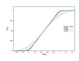
Figure 4: The “population” average arrival distribution function for different values of $T$.

The proof is available in the appendix. Figure 4 depicts $\bar{F}$ for different values of $T$. Notice that the support of the population mean distribution function depends on the value of $T$, and the larger the value of $T$, the earlier and later arrivals can occur to the system (obviously). Interestingly enough, one can also show that the limit population (or mean field) distribution is an average over the individual distribution functions for each user. Following Section 4.1, let $\mathcal{K}:=[0,1]$ represent the universe of all possible users to the queueing system. Then, for $p\in\mathcal{K}$, we know that

$$F_{p}(t):=\frac{t-p+T}{2T}~{}~{}\text{for}~{}~{}p-T\leq t\leq p+T,$$ (29)

is the arrival distribution function of customer $p$. That is, customer $p$ arrives at time $p$, with a uniform uncertainty distribution centered at $p$. The following corollary shows that this population average coincides with the distribution $\bar{F}$ in Proposition 6, when $T\in[0,0.5]$. The proof is a simple integration argument, and is relegated to the appendix.

Corollary 6

Let $F_{p}$ defined in (29) be the arrival distribution associated with user $p\in\mathcal{K}$. Then,

$$\int_{0}^{1}F_{p}(t)m(dp)=\begin{cases}\frac{(t+T)^{2}}{4T},&~{}~{}-T\leq t\leq T,\\ t,&~{}~{}T<t\leq 1-T,\\ \begin{split}&\frac{t+T}{2T}-\frac{t^{2}-T^{2}}{2T}\\ &+\frac{(t-T)^{2}}{4T}-\frac{1}{4T}+(t-T),\end{split}&~{}~{}1-T<t\leq 1+T,\end{cases}$$

where $m(\cdot)$ is the Lebesgue measure on the set $\mathcal{K}$.

This is precisely the condition that needs to be satisfied for the generalized Glivenko-Cantelli result to be true in Theorem 3. Let $F_{n,i}(t):=F(t-\tau_{n,i})$ and extend the support of $F_{n,i}(t)$ to the interval $[-T,1+T]$ such that $F_{n,i}$ is zero outside the interval $[-T+\frac{i}{N_{n}},T+\frac{i}{N_{n}}]$. The scheduled arrival model is, therefore, a special case of the general $\Delta_{(i)}$ traffic model. We claim the following theorem as an immediate consequence of Theorem 3.

Theorem 9

The fluid-scaled arrival process satisfies a functional strong law of large numbers:

$$\bar{A^{n}}\stackrel{{\scriptstyle a.s.}}{{\rightarrow}}\bar{F}\text{ in }(\mathcal{D}_{\lim},U),$$

as $n\to\infty$.

Similar arguments as above we can also prove that the sample covariance function also converges to the average covariance, as obtained in Lemma 3. Since the arguments are similar, we skip the proof and present the final result. The diffusion-scaled arrival process is denoted $\hat{A}^{n}(t):=\sqrt{n}\left(\frac{A^{n}(t)}{n}-\frac{1}{n}\sum_{i=1}^{n}\mathbf{F}(t-\tau_{n,i})\right).$

Theorem 10

The centered arrival process $\hat{A}^{n}$ satisfies a functional central limit theorem,

$$\hat{A}^{n}\Rightarrow\tilde{W}\text{ in }(\mathcal{D}_{lim},U),$$

as $n\to\infty$, where $\tilde{W}\in\mathcal{C}$ is a zero mean Gaussian process with covariance function $K(s,t)$, as obtained in Lemma 3.

As a final note, observe that there is an important distinction between the scheduled arrival and the $\Delta_{(i)}$ pre-limit traffic models. In the latter, the realized arrival times are the ordered statistics of the sampled arrival times, while in the former this is not the case. However, the natural (partial) ordering of the real numbers is all that is required to establish the functional limits, and in the limit as $n\to\infty$ any difference between these models is “washed out”. The results in this and the previous section strongly indicate that, in some sense, the $\Delta_{(i)}$ traffic model is canonical to the study of transitory queueing systems. In the next section we focus on a deeper study of sample path approximations suggested for such models.

5 Conclusions and Future Work

In this paper, we introduced a framework for transitory queueing systems. We define transitory queueing models as those whose arrival process is a finite point process that satisfies (i) the empirical arrival process satisifes a fSLLN and the limit is a well defined probability distribution function, and (ii) the empirical arrival process satisfies a fCLT, converging to a tied down Gaussian process when appropriately centered and scaled. Our attempt is to capture queueing scenarios where the queues are ‘transitory’ either because the queue operates only for a finite time, or because there is only a finite population of customers that will arrive. Such scenarios are very difficult to study via classical queueing analysis, and in some cases even non-stationary Markovian models may not be appropriate.

We first develop fluid and diffusion approximations to the system performance metrics as the population size increases, in a very general setting. More precisely, we only assume that the traffic model satisfies a fluid and diffusion limit, and that the service process is renewal. Under these conditions, we derive a fluid limit to the queue length process and show that it can switch between various regimes. We then derive the diffusion limit of the queue length process in terms of a directional derivative of the Skorokhod reflected fluid ‘netput’ process. This diffusion limit process switches between a free diffusion, a reflected diffusion and the zero process. The weak convergence proof is shown to hold in the $M_{1}$ topology on the space $\mathcal{D}_{\lim}$. A novel feature of the diffusion limit is that it is a function of a Gaussian bridge process and a Brownian motion process. This appears to be a unique observation as such diffusion limits do not appear in the “conventional heavy-traffic” approximations to multi-server queues.

Then, we introduce three natural ‘transitory’ traffic models that satisfy the assumptions. In the $\Delta_{(i)}$ model, a finite population of customers choose (sample) a time of arrival at the queue in an independent manner from distribution functions that are potentially unique to each of them. The customers then enter in order of the sampled arrival times - thus the arrival epochs are ordered statistics. We developed generalizations of the Glivenko-Cantelli and Donsker’s Theorems for triangular arrays, and show that the limit process has an intuitive and interesting interpretation.

Next, we investigated the connection between classical queueing models and the $\Delta_{(i)}/GI/s$ queue. We rigorously show that a conditioned renewal process (appropriately scaled) converges to a Brownian Bridge process a la the i.i.d. sampling $\Delta_{(i)}$ process. This implies that the performance metrics of a (conditioned) $GI/G/s$ queueing model are asymptotically equivalent in distribution to those of the $\Delta_{(i)}/GI/s$ model. We believe this is a new result not reported in the literature before.

Last, we presented fluid and diffusion approximations to a model of scheduled arrivals where the realized arrival epochs are uniformly random around the scheduled arrival epochs. We demonstrate that this model can be viewed as a special case of the $\Delta_{(i)}$ model.

While some non-stationary queueing models can be analyzed by the uniform acceleration (UA) technique, we don’t yet know if this can be used in analyzing ‘transitory’ queueing models as well. Instead, we use the population acceleration (PA) technique. An interesting question is the precise relationship between PA and UA techniques. UA is related to the notion of pointwise stationary approximation (PSA) of the performance metrics of the queue at a fixed time by stationary/ergodic states of an associated notional chain at that time. It is unclear to us if this can be done when pointwise ergodicity is not available.

Finally, we consider this work to be a step towards a comprehensive ‘theory of transitory stochastic networks’. Our focus is next going to be to extend the current theory to ‘transitory queueing networks’ with networks of $\Delta_{(i)}/GI/1$ queues. Moreover, obtaining stochastic process limits in the non-degenerate slowdown regime [2] (i.e., when the number of servers $s_{n}=n^{\alpha}$ for $\alpha\in[0,1]$) would be very useful in developing “non-conventional” large population approximations to transitory many-server systems. Another interesting class of problems is in the development of large and moderate deviation analyses of transitory queueing systems, something that we believe will be quite different from conventional queues. Last, while we have mostly focused on the single class setting, there are very interesting questions in the context of multi-class transitory systems, for instance in designing optimal schedulers.

6 Proofs of Lemmas and Theorems

6.1 Proof of Lemma 1

(i). $\mathcal{D}$ is a subspace under the relative topology $\tau_{r}:=\{A\cap\mathcal{D}|A\in\tau_{\lim}\}$, where $\tau_{\lim}$ is the topology induced by the $J_{1}$ metric on $\mathcal{D}_{\lim}$. Then, it follows that $\mathscr{D}=\mathscr{D}_{r}:=\{\mathcal{D}\cap A|A\in\mathscr{D}_{\lim}\}$. To see this, note that $\mathscr{D}_{r}$ contains all possible open sets of $\mathcal{D}$ (since these are elements of $\mathscr{D}_{\lim}$) and $\mathscr{D}_{r}$ is a $\sigma$-algebra. This implies that $\mathscr{D}\subseteq\mathscr{D}_{r}$ since the Borel $\sigma$-algebra is the smallest to contain all open subsets of $\mathcal{D}$. In the opposite direction, by since $\mathcal{D}$ is a subspace, the injection map $\iota:\mathcal{D}\to\mathcal{D}_{\lim}$ is a homeomorphism, implying that for any Borel set $A\in\mathscr{D}_{\lim}$, $\iota^{-1}(A)$ is Borel in $\mathcal{D}$. But, the inclusion map is clearly $\iota^{-1}(A)=A\cap\mathcal{D}$ by definition. Therefore $\mathscr{D}_{r}\subseteq\mathscr{D}$.

This implies that for any $D\in\mathscr{D}_{\lim}$, $\mathbb{P}(x\in D)=\mathbb{P}(x\in D\cap\mathcal{D})$ is well defined since $x$ is defined with respect to $(D,\mathscr{D})$. This extends the definition of the measure induced by $x$ to $\mathcal{D}_{\lim}$.

(ii) Now, let $G\subset\mathcal{D}_{\lim}$ be any closed subset. Then, we have

$$\mathbb{P}(x_{n}\in G)=\mathbb{P}(x_{n}\in G\cap\mathcal{D})+\mathbb{P}(x_{n}\in G\cap\mathcal{D}^{c})=\mathbb{P}(x_{n}\in G\cap\mathcal{D}),$$

where $\mathcal{D}^{c}$ is the complement set. Let $E:=G\cap\mathcal{D}$, and note that $\mathcal{D}\backslash E=\mathcal{D}\cap E^{c}=\mathcal{D}\cap G^{c}$. This implies that $\mathcal{D}\backslash E$ is open in the relative topology on $\mathcal{D}$ since $G^{c}$ is open in $\tau_{\lim}$. Now, using the fact that $x_{n}\Rightarrow x$ in $(\mathcal{D},J_{1})$ and part (iii) of Theorem 2.1 of [3] we have $\limsup_{n\to\infty}\mathbb{P}(x_{n}\in G\cap\mathcal{D})\leq\mathbb{P}(x\in G\cap\mathcal{D})$. This implies that

$$\limsup_{n\to\infty}\mathbb{P}(x_{n}\in G)\leq\mathbb{P}(x\in G\cap\mathcal{D})=\mathbb{P}(x\in G),$$

where the last equality follows by the fact that $x$ concentrates on $\mathcal{D}$. By part (i) of Theorem 2.1 of [3], it follows that $x_{n}\Rightarrow x$ in $(\mathcal{D}_{\lim},J_{1})$ as $n\to\infty$.   

6.2 Statement and Proof of Lemma 5

Lemma 5

As $n\rightarrow\infty$,

$$\hat{X}^{n}\Rightarrow\hat{X}\,:=\,\tilde{W}-W\circ\bar{B}~{}\text{ in }(\mathcal{D}_{\lim},J_{1})$$ (30)

where $\bar{B}$ is defined in (8), and $\tilde{W}$ and $W$ are mutually independent Gaussian bridge and Brownian motion processes respectively, as defined in Proposition 1

Proof: Fix $j\in\{1,\ldots,N\}$. Recall that $B_{j}^{n}(t)\leq t,\forall t\in[0,\infty)$, implying that $S_{j}^{n}\circ B_{j}^{n}\in\mathcal{D}_{\lim}$. Using (5) in Proposition 1, Corollary 1 and the random time change theorem (see, for example, Section 17 of [3]), it follows that $\sqrt{N_{n}}\bigg{(}\frac{S_{j}^{n}\circ B_{j}^{n}}{N_{n}}-\mu B_{j}^{n}\bigg{)}\Rightarrow\sigma\mu^{3/2}W_{j}\circ\bar{B}_{j}.$  Now, it follows from Proposition 1 and the weak limit just proved that $\hat{X}^{n}\Rightarrow\hat{X}(t)\,:=\,\tilde{W}-\sum_{j=1}^{s}\sigma\mu^{3/2}W_{j}\circ\bar{B}_{j}\stackrel{{\scriptstyle d}}{{=}}\tilde{W}-W\circ\bar{B},$ where the final equality follows from the fact that the sum of independent Brownian motions is equal in distribution to a Brownian motion.   

6.3 Statement and Proof of Lemma 6.

This result is a consequence of Theorem 9.5.1 of [56]. A version of this result is also proved in [22].

Lemma 6 (Directional derivative reflection mapping lemma)

Let $x\in\mathcal{D}$ and $y\in\mathcal{C}$ be real-valued functions on $[0,\infty)$, and $\Psi(z)(t)=\sup_{0\leq s\leq t}(-z(s))$, for any process $z\in\mathcal{D}_{\lim}$. Let $\{y_{n}\}\subset\mathcal{D}_{\lim}$ be a sequence of functions such that $y_{n}\stackrel{{\scriptstyle a.s.}}{{\rightarrow}}y$ as $n\rightarrow\infty$. Then, with respect to Skorokhod’s $M_{1}$ topology, $\tilde{y}_{n}:=\Psi(\sqrt{N_{n}}x+y_{n})-\sqrt{N_{n}}\Psi(x)\longrightarrow\tilde{y}:=\sup_{s\in\nabla_{t}^{x,L}}(-y(s))\vee\sup_{s\in\nabla_{t}^{x,R}}(-y(s))$ as $n\rightarrow\infty$, where $\nabla_{t}^{x,\cdot}$ are defined in Definition 2.

Rewrite $\tilde{y}_{n}$ as

$$\tilde{y}_{n}=(\Psi(\sqrt{n}x+y_{n})-\Psi(\sqrt{n}x+y))-(\Psi(\sqrt{n}x+y)-\sqrt{n}\Psi(x)).$$

Now, using the fact that the Skorokhod reflection map is Lipschitz continuous under the uniform metric (see Lemma 13.4.1 and Theorem 13.4.1 of [57]) we have

$$(\Psi(\sqrt{n}x+y_{n})-\Psi(\sqrt{n}x+y))\leq\|y_{n}-y\|,$$

where $\|\cdot\|$ is the uniform metric. It follows that

$$\tilde{y}_{n}\leq\|y_{n}-y\|+(\Psi(\sqrt{n}x+y)-\sqrt{n}\Psi(x)),$$

Now, by Theorem 9.5.1 of [56] we know that as $n\rightarrow\infty$

$$(\Psi(\sqrt{n}x+y)-\sqrt{n}\Psi(x))\stackrel{{\scriptstyle a.s.}}{{\rightarrow}}\tilde{y},\text{ in }(\mathcal{D}_{\lim},M_{1}).$$

Using this result, and the fact that by hypothesis $y_{n}$ converges to $y$ in $(\mathcal{D}_{\lim},U)$ we have

$$\tilde{y}_{n}\stackrel{{\scriptstyle a.s.}}{{\rightarrow}}\tilde{y},\text{ in }(\mathcal{D}_{\lim},M_{1}).$$

 

6.4 Proof of Proposition 4.

Recall that $\tilde{y}_{n}$ converges to $\tilde{y}$ in the $M_{1}$ topology, from Lemma 6. Now, consider a path of $y$ that is non positive at $\tau$. Thus, the limit process $\tilde{y}$ has a discontinuity at $\tau$ such that $\tilde{y}(\tau)>\tilde{y}(\tau+)$. Note that the process path is left continuous at $\tau$. Assume that $\tilde{y}(\tau)-\tilde{y}(\tau+)>\delta>0$, and it follows that $\tilde{y}(\tau)=-y(\tau)>\delta$ (since $\tilde{y}(\tau+)=0$). Fix an $\epsilon>0$ such that $\delta>\epsilon$. Now, by the continuity of $y$, there exists $\eta>0$ such that $\sup_{t\in[\tau-\eta,\tau+\eta]}|y(t)-y(\tau)|\leq\frac{\epsilon}{4}$. Then, there also exists a $n_{0}$ such that for all $n>n_{0}$, $0\geq-\sqrt{n}x(t)>-\frac{e}{4}$ for $t\in[\tau-\eta,\tau]$.

Then, for any $t\in[\tau-\eta]$ it follows that

$$-\sqrt{n}x(t)-y(t)+y(\tau)>-\frac{\epsilon}{2}.$$

This implies that $-\sqrt{n}x(t)-y(t)>\delta-\frac{\epsilon}{2}>\frac{e}{2},$ since $\delta>\epsilon$. It follows that $\Psi(\sqrt{n}x+y)>\frac{\epsilon}{2}$ for all time points $t\in[\tau-\eta,\tau]$. Thus, it cannot be the case that uniform convergence is possible on any compact set of $[-T_{0},\infty)$. Furthermore, consider any sequence $\{\lambda_{n}\}\subseteq\Lambda$. Then, for large $n$, by assumption, $\lambda_{n}$ is uniformly close to the identity map. Thus, any distortion introduced by the homeomorphism will be minimal, and the same argument will show that it cannot be the case that, for any fixed $\epsilon>0$, $\|\tilde{y}_{n}\circ\lambda_{n}-\tilde{y}\circ e\|\leq\frac{\epsilon}{2}$ for large $n$, and there is a set of points determined by $\eta$ (due to the continuity of $y$) where it is the case that $|(\tilde{y}_{n}\circ\lambda_{n})(t)-(\tilde{y}\circ e)|>\frac{\epsilon}{2}$.   

6.5 Proof of Lemma 2

For each $n\in\mathbb{N}$ we have $F_{n,i}=\Upsilon\left(\frac{i}{N_{n}}\right)$, $i=1,\ldots,N_{n}$. Therefore, (26) can be rewritten as $\bar{F}_{n}(t)=\frac{1}{N_{n}}\sum_{i=1}^{N_{n}}\Upsilon\left(\frac{i}{N_{n}}\right)(t),$ and we prove that $\left\|\frac{1}{N_{n}}\sum_{i=1}^{N_{n}}\Upsilon\left(\frac{i}{N_{n}}\right)(t)-\int_{[0,1]}\Upsilon(s)(t)m(ds)\right\|_{[0,1]}\to 0$ as $n\to\infty$. Notice that $\bar{F}(t)$ is a Riemann-Stieltjes integral with respect to the Lebesgue measure. Therefore, it is natural to view $\bar{F}_{n}$ as a Riemann-Stieltjes (pre-limit) sum. For a fixed $t\in[0,1]$, therefore, we show that the Riemann sums converge to the Riemann-Stieltjes integral.

Let $M_{i}(t):=\sup\Upsilon(x)(t)$ and $m_{i}(t):=\inf\Upsilon(x)(t)$ for all $x\in\left[\frac{i-1}{N_{n}},\frac{i}{N_{n}}\right]$ and $i=1,\ldots,N_{n}$. We define the “upper” and “lower” Riemann sums as (respectively) $U_{n}(t):=\sum_{i=1}^{N_{n}}M_{i}\left(\frac{i}{N_{n}}-\frac{i-1}{N_{n}}\right)$ and $N_{n}(t):=\sum_{i=1}^{N_{n}}m_{i}\left(\frac{i}{N_{n}}-\frac{i-1}{N_{n}}\right).$ Clearly, for every $\epsilon>0$ and large enough $n$, $U_{n}(t)-N_{n}(t)<\epsilon$ due to the Lipschitz continuity property assumed for $\Upsilon$. This is tantamount to showing that the bound holds for at least one possible partition of $[0,1]$. Then, by Theorem 6.6 of [49], it follows that the limit exists and is equal to $\bar{F}(t)$. The Lipschitz continuity property implies that the limit clearly holds for all $t\in S$, implying uniform convergence.   

6.6 Proof of Lemma 3

The first summation in the definition of $K_{n}(s,t)=\frac{1}{N_{n}}\sum_{i=1}^{N_{n}}F_{n,i}(s\wedge t)-\frac{1}{N_{n}}\sum_{i=1}^{N_{n}}F_{n,i}(s)F_{n,i}(t)$ converges to $\int_{\mathcal{K}}F_{p}(s\wedge t)m(dp)$ as $n\to\infty$ by Lemma 2. The second summation converges as well by using the same Riemann-Stieltjes summation argument used in the proof of Lemma 2, and the limit is $\int_{\mathcal{K}}F_{p}(t)F_{p}(s)m(dp)$.   

6.7 Proof of Theorem 3

First, fix $t\in[0,1]$ and $\epsilon>0$. Consider

$$\mathbb{P}\left(\left|\bar{A}^{n}(t)-\bar{F}_{n}(t)\right|>\epsilon\right) = \mathbb{P}\left(\left|\frac{1}{N_{n}}\sum_{i=1}^{N_{n}}\left(\mathbf{1}_{\{T_{n,i}\leq t\}}-\Upsilon(i/N_{n})(t)\right)\right|>\epsilon\right)$$ (31)

$$\leq \frac{1}{\epsilon^{4}N_{n}^{4}}\mathbb{E}\left|\sum_{i=1}^{N_{n}}\left(\mathbf{1}_{\{T_{n,i}\leq t\}}-\Upsilon(i/N_{n})(t)\right)\right|^{4}$$

$$= \begin{split}&\frac{1}{\epsilon^{4}N_{n}^{4}}\sum_{i=1}^{N_{n}}\mathbb{E}\left|\mathbf{1}_{\{T_{n,i}\leq t\}}-\Upsilon(i/N_{n})(t)\right|^{4}\\ &+\frac{12}{\epsilon^{4}N_{n}^{4}}\sum_{i=1}^{N_{n}-1}\sum_{j=i+1}^{N_{n}}\mathbb{E}\left|\mathbf{1}_{\{T_{n,i}\leq t\}}-\Upsilon(i/N_{n})(t)\right|^{2}\mathbb{E}\left|\mathbf{1}_{\{T_{n,j}\leq t\}}-\Upsilon(j/N_{n})(t)\right|^{2}\end{split}$$

$$\leq \begin{split}\frac{1}{\epsilon^{4}N_{n}^{4}}\sum_{i=1}^{N_{n}}\Upsilon(i/N_{n})(t)&(1-\Upsilon(i/N_{n})(t))\\ &+\frac{12}{\epsilon^{4}N_{n}^{4}}\left(\sum_{i=1}^{N_{n}}\Upsilon(i/N_{n})(t)(1-\Upsilon(i/N_{n})(t))\right)^{2},\end{split}$$

where the last inequality follows due to the fact that the terms that remain in the expansion of $\mathbb{E}\left|\sum_{i=1}^{N_{n}}\left(\mathbf{1}_{\{T_{n,i}\leq t\}}-\Upsilon(i/N_{n})(t)\right)\right|^{4}$ are $\sum_{i=1}^{N_{n}}\mathbb{E}|\mathbf{1}_{\{T_{n,i}\leq t\}}-\Upsilon(i/N_{n})(t)|^{2}$ and cross products $\sum_{i=1}^{N_{n}-1}\sum_{j=i+1}^{N_{n}}\mathbb{E}|\mathbf{1}_{\{T_{n,i}\leq t\}}-\Upsilon(i/N_{n})(t)|^{2}\mathbb{E}|\mathbf{1}_{\{T_{n,j}\leq t\}}-\Upsilon(j/N_{n})(t)|^{2}$. From Lemma 3 it follows that (31) is bounded above by $\frac{C}{\epsilon^{4}N_{n}^{2}}$. Therefore, by the Borel-Cantelli Lemma, $\sum_{n=1}^{\infty}\mathbb{P}\left(\left|\bar{A}^{n}(t)-\bar{F}_{n}(t)\right|>\epsilon\right)<\infty,$ implying that $\mathbb{P}\left(\left|\bar{A}^{n}(t)-\bar{F}_{n}(t)\right|>\epsilon~{}i.o.\right)=0$. Combining this result with Lemma 2 proves that $\bar{A}^{n}$ converges to $\bar{F}$ almost surely pointwise.

Next, consider a uniform partition of the support $[0,1]$, and suppose $\frac{j-1}{M}\leq t\leq\frac{j}{M}$, where $j=1,\ldots,M$ and $M$ is the size of the partition. Then, for fixed $n$, $\bar{A}^{n}\left(\frac{j-1}{M}\right)\leq\bar{A}^{n}\left(t\right)\leq\bar{A}^{n}\left(\frac{j}{M}\right),$ implying that $\frac{1}{N_{n}}\sum_{i=1}^{N_{n}}\left(\mathbf{1}_{\{T_{n,i}\leq j-1/M\}}-F_{n,i}(j-1/M)\right)$

$$\begin{split}&\leq\frac{1}{N_{n}}\sum_{i=1}^{N_{n}}\left(\mathbf{1}_{\{T_{n,i}\leq t\}}-F_{n,i}(t)\right)+\frac{1}{N_{n}}\sum_{i=1}^{N_{n}}\left(F_{n,i}(j/M)-F_{n,i}(j-1/M)\right)\\ &\leq\frac{1}{N_{n}}\sum_{i=1}^{N_{n}}\left(\mathbf{1}_{\{T_{n,i}\leq j/M\}}-F_{n,i}(j/M)\right).\end{split}$$

For each $M$, there exists $n_{M}$ such that for all $n\geq n_{M}$ $\left|F_{n,i}(j/M)-F_{n,i}(j-1/M)\right|\leq\frac{1}{M}$. Further, for $\epsilon>0$, there exists $n^{{}^{\prime}}_{M}$ such that for all $n\geq\max(n_{M},n_{M}^{{}^{\prime}})$,

$$\left|\frac{1}{N_{n}}\sum_{i=1}^{N_{n}}\left(\mathbf{1}_{\{T_{n,i}\leq k\}}-F_{n,i}(k)\right)\right|<\epsilon,$$

where $k=j-1/M\text{ or }j/M$. It follows that

$$\sup_{t\in[0,1]}\left|\frac{1}{N_{n}}\sum_{i=1}^{N_{n}}\left(\mathbf{1}_{\{T_{n,i}\leq t\}}-F_{n,i}(t)\right)\right|<2(\epsilon+\frac{1}{M}).$$

Since $\epsilon$ is arbitrary, letting $M\to\infty$ the desired result follows.   

6.8 Proof of Theorem 4

We first prove pointwise convergence by verifying the sufficiency of the Lyapunov Central Limit Theorem (Theorem 7.3 [3]). Fix $t\in[0,1]$ and let $\delta>0$, and consider

$$\frac{\sum_{i=1}^{N_{n}}E|F_{n,i}(t)-\mathbf{1}_{\{T_{n,i}\leq t\}}|^{2+\delta}}{\left(\sum_{i=1}^{N_{n}}F_{n,i}(t)(1-F_{n,i}(t))\right)^{2+\delta}}.$$

Dividing the numerator and denominator by $1/N_{n}^{2+\delta}$, note that the denominator converges to $(\bar{F}(t))^{2+\delta}$ as a consequence of Lemma 2. Consider the numerator alone,

$$\frac{1}{N_{n}^{2+\delta}}\sum_{i=1}^{N_{n}}E|F_{n,i}(t)-\mathbf{1}_{\{T_{n,i}\leq t\}}|^{2+\delta}\leq\frac{2^{\delta}}{N_{n}^{2+\delta}}\sum_{i=1}^{N_{n}}F_{n,i}(t)(1-F_{n,i}(t)),$$

which tends to 0 as $n\to\infty$. The Lyapunov CLT implies that

$$\frac{\sum_{i=1}^{N_{n}}(F_{n,i}(t)-\mathbf{1}_{\{T_{n,i}\leq t\}})}{\sqrt{\sum_{i=1}^{N_{n}}F_{n,i}(t)(1-F_{n,i}(t))}}=\frac{\sum_{i=1}^{N_{n}}(F_{n,i}(t)-\mathbf{1}_{\{T_{n,i}\leq t\}}}{\sqrt{N}_{n}}\times\frac{\sqrt{N_{n}}}{\sqrt{\sum_{i=1}^{N_{n}}F_{n,i}(t)(1-F_{n,i}(t))}}\Rightarrow\mathcal{N}(0,1).$$

By Lemma 3 it follows that $\frac{\sum_{i=1}^{N_{n}}(F_{n,i}(t)-\mathbf{1}_{\{T_{n,i}\leq t\}}}{\sqrt{N}_{n}}\Rightarrow\tilde{W}(t):=\sqrt{K(t,t)}\mathcal{N}(0,1)$. Next, using the Cramer-Wold device it is straightforward to argue that $(\hat{A}^{n}(t_{1}),\ldots,\hat{A}^{n}(t_{k}))\Rightarrow(\tilde{W}(t_{1}),\ldots,\tilde{W}(t_{k}))$ where $(t_{1},\ldots,t_{k})\in[0,1]^{k}$ for all $k\in\mathbb{N}$.

Finally, we verify the sufficiency of Theorem 15.6 of [3] to show that $\hat{A}^{n}\Rightarrow\tilde{W}$ in $(\mathcal{D},J_{1})$. To ease the notation, let $X_{n,i}(t):=(\mathbf{1}_{\{T_{n,i}\leq t\}}-F_{n,i}(t))$. By Chebyshev’s inequality, for any $\lambda>0$ and $t_{1}\leq t\leq t_{2}\in[0,1]$, $\lambda^{4}\mathbb{P}(|\hat{A}^{n}(t)-\hat{A}^{n}(t_{1})|\geq\lambda,|\hat{A}^{n}(t)-\hat{A}^{n}(t_{2})|\geq\lambda)$

$$\leq E\left[(\hat{A}^{n}(t_{1})-\hat{A}^{n}(t))^{2}(\hat{A}^{n}(t_{1})-\hat{A}^{n}(t))^{2}\right].$$

$$= \frac{1}{N_{n}^{2}}E\left[\left|\sum_{i=1}^{N_{n}}(X_{n,i}(t)-X_{n,i}(t_{1}))\right|^{2}\left|\sum_{i=1}^{N_{n}}(X_{n,i}(t_{2})-X_{n,i}(t))\right|^{2}\right]$$

$$= \frac{1}{N_{n}^{2}}E\left[\begin{split}&\sum_{i=1}^{N_{n}}|X_{n,i}(t)-X_{n,i}(t_{1})|^{2}\sum_{i=1}^{N_{n}}|X_{n,i}(t_{2})-X_{n,i}(t)|^{2}\\ &+2\sum_{i<j}(X_{n,i}(t_{2})-X_{n,i}(t))(X_{n,j}(t_{2})-X_{n,j}(t))\sum_{l=1}^{N_{n}}|X_{n,l}(t)-X_{n,l}(t_{1})|^{2}\\ &+2\sum_{i<j}(X_{n,i}(t)-X_{n,i}(t_{1}))(X_{n,j}(t)-X_{n,j}(t_{1}))\sum_{l=1}^{N_{n}}|X_{n,l}(t_{2})-X_{n,l}(t)|^{2}\\ &+4\sum_{i<j}(X_{n,i}(t)-X_{n,i}(t_{1}))(X_{n,j}(t)-X_{n,j}(t_{1}))\sum_{i<j}(X_{n,i}(t_{2})-X_{n,i}(t))(X_{n,j}(t_{2})-X_{n,j}(t))\end{split}\right]$$

$$\leq \begin{split}&\frac{1}{N_{n}}\sum_{i=1}^{N_{n}}\left[(F_{n,i}(t)-F_{n,i}(t_{1}))(F_{n,i}(t_{2})-F_{n,i}(t))(1-F_{n,i}(t)+F_{n,i}(t_{1}))(1-F_{n,i}(t_{2})+F_{n,i}(t))\right]^{1/2}\\ &+2\frac{1}{N_{n}^{2}}\sum_{i<j}\left[(F_{n,i}(t)-F_{n,i}(t_{1}))(F_{n,j}(t_{2})-F_{n,j}(t))(1-F_{n,i}(t)+F_{n,i}(t_{1}))(1-F_{n,j}(t_{2})+F_{n,j}(t))\right]\\ &+4\sum_{i<j}(F_{n,i}(t)-F_{n,i}(t_{1}))(F_{n,i}(t_{2})-F_{n,i}(t))(F_{n,j}(t)-F_{n,j}(t_{1}))(F_{n,j}(t_{2})-F_{n,j}(t))\end{split}$$

$$\leq C$$

where $C\geq 8$ and the bound is true for all $t_{2}>t_{1}$. Theorem 15.6 of [3] shows that if $\mathbb{P}(|\hat{A}^{n}(t)-\hat{A}^{n}(t_{1})|\geq\lambda,|\hat{A}^{n}(t)-\hat{A}^{n}(t_{2})|\geq\lambda)\leq(G(t_{2})-G(t_{1}))^{2\alpha},$ where $G$ is a non-decreasing function on $[0,1]$ and $\alpha>1/2$, then $\hat{A}^{n}$ converges weakly to a limit in $(\mathcal{D},J_{1})$. Therefore, $\hat{A}^{n}\Rightarrow\tilde{W}$ as $n\to\infty$. The convergence in $(\mathcal{D}_{\lim},J_{1})$ follows by an application of part (ii) of Lemma 1. Finally, by part (ii) of Theorem 1.1 of [50] we know that $\tilde{W}$ has continuous sample paths, implying that $A^{n}\Rightarrow\tilde{W}$ in $(\mathcal{D}_{\lim},U)$, thus completing the proof.   

6.9 Proof of Theorem 5

Let $\mathbf{T}:=\{T_{i},\,i=1,\ldots,n\}$ be a collection of i.i.d. random variables, with distribution function $F$ (defined in (28)). Let $A^{n}(t):=\sum_{i=1}^{n}\mathbf{1}_{\{T_{i}\leq t\}}$ and $\hat{A}^{n}(t):=\sqrt{n}\left(\frac{A^{n}(t)}{n}-F(t)\right)$ be the empirical process associated with $\mathbf{T}$. For a fixed $n\geq 1$ and $x\in\mathbb{R}$ we have

$$\mathbb{P}(\hat{M}_{n}(t)\leq x|M(T)=n)=\mathbb{P}(M(t)\leq x\sqrt{n}+nF(t)|M(T)=n).$$

The OS property implies that $M(t)|_{\{M(T)=n\}}\stackrel{{\scriptstyle d}}{{=}}A^{n}(t)$. Proposition 3 implies that

$$\mathbb{P}(M(t)\leq x\sqrt{n}+nF(t)|M(T)=n) = \mathbb{P}(A^{n}(t)\leq x\sqrt{n}+nF(t))$$

$$= \mathbb{P}(\hat{A}^{n}(t)\leq x)$$

$$\Rightarrow (W^{0}\circ F)(t)$$

proving the pointwise convergence of the process $\hat{M}_{n}$. It is also well known that for any $0<t_{1}<\cdots<t_{d}<T$, $\mathbb{P}(M(t_{1})=n_{1},\ldots,M(t_{d})=n_{d}|M(T)=n)=\mathbb{P}(A^{n}(t_{1})=n_{1},\ldots,A^{n}(t_{d})=n_{d})$, where $n_{1}+\cdots n_{d}=n$, so the fact that $(\hat{A}^{n}(t_{1}),\ldots,\hat{A}^{n}(t_{d}))\Rightarrow(W^{0}\circ F)(t_{1}),\cdots,(W^{0}\circ F)(t_{d}))$ implies that the finite dimensional distrbutions of $\hat{M}_{n}$ converge to the same limit. The tightness of $\hat{M}_{n}$ is implied directly by that of $\hat{A}^{n}$, so by Theorem 8.1 of [3] the theorem is proved.   

6.10 Proof of Proposition 5

Let $\{x_{1},\ldots,x_{n}\}\subset[0,T]$ be such that $0\leq x_{1}<x_{2}<\cdots<x_{n}\leq T$. Consider the measure of the event $\{\xi_{1}\in dx_{1},\cdots,\xi_{n}\in dx_{n}\}\in\mathcal{F}$,

$$\begin{split}P(\xi_{1}\in dx_{1},&\cdots,\xi_{n}\in dx_{n}|M(T)=n)\\ =&\frac{P((\xi_{1}\in dx_{1},\cdots,\xi_{n}\in dx_{n}),M(T)=n)}{P(M(T)=n)}.\end{split}$$

Recall that $\{M(T)=n\}=\{\sum_{l=1}^{n}\xi_{l}\leq T<\sum_{l=1}^{n+1}\xi_{l}\}$, implying that we have:

$$\begin{split}&\frac{P((\xi_{1}\in dx_{1},\cdots,\xi_{n}\in dx_{n}),M(T)=n)}{P(M(T)=n)}\\ =&\frac{P(\xi_{1}\in dx_{1},\ldots\xi_{n}\in dx_{n},\sum_{l=1}^{n}\xi_{l}\leq T,\sum_{l=1}^{n}\xi_{l}+\xi_{n+1}>T)}{P(M(T)=n)}.\end{split}$$

Using the fact that under the measure $\mathbb{P}$, $\xi_{i}$ are i.i.d. random variables, it follows that the measure of the joint event is invariant under any permutation of the first $n$ random variables. That is, if $\pi(\cdot)$ is a permutation of $\{1,\ldots,n\}$, then we have

$$\begin{split}&\frac{P((\xi_{1}\in dx_{1},\cdots,\xi_{n}\in dx_{n}),M(T)=n)}{P(M(T)=n)}\\ =&\frac{P(\xi_{\pi(1)}\in dx_{1},\ldots\xi_{\pi(n)}\in dx_{n},\sum_{l=1}^{n}\xi_{\pi(l)}\leq T,\sum_{l=1}^{n}\xi_{\pi(l)}+\xi_{n+1}>T)}{P(M(T)=n)},\end{split}$$

which is equal to $P_{n}(\xi_{\pi(1)}\in dx_{1},\ldots\xi_{\pi(n)}\in dx_{n})$. Next, suppose that $\pi(\cdot)$ is a permutation of $\{1,\ldots,n+1\}$. Then, it is possible that the event $\sum_{i=1}^{n}\xi_{\pi(l)}>T$, since $\xi_{n+1}>T-\sum_{l=1}^{n}\xi_{l}>0$, conditionally on $\{M(T)=n\}$. Thus, $\Xi_{n}$ cannot be extended to a larger collection of exchangeable random variables, implying that it is finitely exchangeable.   

6.11 Conditioned Renewal Process: Lemmata

6.11.1 Sample Space Construction

We assume that the underlying sample space $\Omega,\mathcal{F},\mathbb{P}$ is rich enough to support a sequence of (jointly) independent stochastic processes $\{M_{n}\},\,n\geq 1$, such that they are each indistinguishable from $M$. That is, for any $n\geq 1$, $\mathbb{P}(M_{n}(t)\not=M(t),\,\forall t\geq 0)=0$. For a fixed $n\geq 1$ and $T>0$, we define the restricted sample space, $(\Omega_{n},\mathcal{F}_{n},\mathbb{P}_{n})$, where $\Omega_{n}=\Omega\cap\{M_{n}(T)=n\}$, $\mathcal{F}_{n}:=\sigma\{A\cap\{M_{n}(T)=n\}:A\in\mathcal{F}\}$ and $\mathbb{P}_{n}(B):=\frac{P(B)}{P(M_{n}(T)=n)}$ for any $B\in\mathcal{F}_{n}$. Clearly $\{\{M(T)=n\}$ $n\geq 1\}$ forms a partition of $\Omega$. The following claim shows that this property ($\mathbb{P}-a.s.$) extends to the collection $\{\Omega_{n}\}$.

Lemma 7

$\{\Omega_{n}\}$ $n\geq 1$ forms a $\mathbb{P}-a.s.$ partition of $\Omega$.

Proof: For a fixed $n\geq 1$ and $m\in\mathbb{N}$, $\{M_{n}(T)=m\}$, forms a partition of $\Omega$, as do $\{M(T)=m\}$. By assumption $M_{n}$ and $M$ are indistinguishable from each other. It is straightforward to deduce that $\mathbb{P}(\{M_{n}(T)=m\}\Delta\{M(T)=m\})=0$, implying that $\{M_{n}(T)=m\}=\{M(T)=m\}\,\mathbb{P}-a.s.$ for every $m\in\mathbb{N}$.

Now, consider the collection of sets $\{\{M_{n}(T)=n\}\}$ $n\geq 1$. For brevity, let $A_{n}:=\{M_{n}(T)=n\}$ and $B_{n}:=\{M(T)=n\}$. We have

$$\left(\cup_{n\geq 1}\{M_{n}(T)=n\}\right)\Delta\left(\cup_{n\geq 1}\{M(T)=n\}\right) = \left(\cup_{n\geq 1}A_{n}\right)\Delta\left(\cup_{n\geq 1}B_{n}\right)$$

$$= \cup_{l\geq 1}\left(\cap_{n\geq 1}(B_{l}\cap A_{n}^{c})\right).$$

By the assumption of indistinguishability, $\mathbb{P}(B_{l}\cap A_{l}^{c})=0$, implying that $\mathbb{P}(\cap_{n\geq 1}(B_{l}\cap A_{n}^{c}))=0$, for every $l\geq 1$. Therefore,

$$\mathbb{P}\left(\cup_{n\geq 1}\{M_{n}(T)=n\}\right)\Delta\left(\cup_{n\geq 1}\{M(T)=n\}\right)=0.$$

By virtue of the fact that $\cup_{n\geq 1}\{M(T)=n\}=\Omega$ it follows that $\{\{M_{n}(T)=n\}\},\,n\geq 1$ forms a partition of $\Omega$ $\mathbb{P}-a.s.$   

Next, we construct a new product space from the restricted sample spaces $(\Omega_{n},\mathcal{F}_{n},\mathbb{P}_{n})$ as follows. Let, $\bar{\Omega}:=\Omega_{1}\times\Omega_{2}\times\cdots$, so that $A\subset\bar{\Omega}=A_{1}\times A_{2}\times\cdots$ for sets $A_{n}\subset\Omega_{n}$. The product $\sigma-$algebra, $\bar{\mathcal{F}}:=\mathcal{F}_{1}\otimes\mathcal{F}_{2}\otimes\cdots$ is the $\sigma-$algebra generated from cylinder sets of the type $R=\{(\omega_{1},\omega_{2},\cdots)\in\bar{\Omega}|\omega_{i_{1}}\in A_{i_{1}},\cdots,\omega_{i_{k}}\in A_{i_{k}}\}$, where $(i_{1},\ldots,i_{l})$ is an arbitrary subset of $\mathbb{N}$ of size $k\geq 1$ and $A_{i_{n}}\in\mathcal{F}_{n}$. The existence of such a product $\sigma-$algebra is well-justified by Proposition 1.3 in [14]. Finally, we define $\bar{\mathbb{P}}(R)=\Pi_{i=1}^{k}\mathbb{P}_{i_{l}}(A_{i_{l}})$, for the cylinder sets. This extends to $\bar{P}=\mathbb{P}_{1}\times\mathbb{P}_{2}\times\cdots$, which is the natural product measure on the measure space $(\bar{\Omega},\bar{\mathcal{F}})$, by standard arguments showing that the measure is countably additive on $\bar{\mathcal{F}}$. The definition of the Lebesgue integral on the space $(\bar{\Omega},\bar{\mathcal{F}},\bar{\mathbb{P}})$ now follows from standard definitions of integration on product spaces. However, we introduce some notation to ease our burden. In particular, consider a function defined in the following manner: $\bar{X}:=X\times\Pi_{l\not=n}\mathbb{I}_{\{\Omega_{l}\}}$, where $X$ is measurable and integrable with respect to $(\Omega_{n},\mathcal{F}_{n},\mathbb{P}_{n})$, and $\mathbb{I}_{\{\cdot\}}$ is the indicator function. Then

$$E_{\bar{\mathbb{P}}}[\bar{X}]=\int_{\Omega_{n}}Xd\mathbb{P}_{n}\int_{\Pi_{l\not=n}}\mathbb{I}_{\{\Omega_{l}\}}d\mathbb{P}_{l}$$

is well-defined, and we write this as $E_{\bar{\mathbb{P}}}[X]$, where it is to be understood that the integration is actually of $\bar{X}$.

6.11.2 Preliminary Lemmata

Armed with the new product space, we can now proceed to the proof of the diffusion limit. We define the collection of random variables, $\Xi_{n}:=(\xi_{n,1},\cdots,\xi_{n,n})$ to be “conditioned” inter-arrival times of the renewal process $M_{n}$ provided that

$$M_{n}(t)=\sup\{k\geq 0|\sum_{i=1}^{k}\xi_{n,i}\leq t\},$$

for $t\leq T$ and $\sum_{i=1}^{n}\xi_{n,i}\leq T$. From Proposition 5 it follows that $\Xi_{n}$ forms an exchangeable array, under the measure $\mathbb{P}_{n}$. Furthermore, under the measure $\bar{\mathbb{P}}$, $\Xi_{n}$ and $\Xi_{m}$ ($m\not=n$) are independent of each other (by the definition of the product measure). The following lemma characterizes the mean and variance of the inter-arrival times, for a fixed $n$. Intuitively, one should expect the mean and variance to decrease to 0 as $n\to\infty$, as there are a larger number of variables being packed into a fixed interval ($T$ is fixed, of course). This characterization is important in proving the diffusion limit. We start with a simple lemma.

Lemma 8

Let $\{f_{n}\}$ be a sequence of non-negative, measurable, functions. Let $P$ be a given measure. Assume: a) $\int f_{n}dP\to 0$ as $n\to\infty$, b) $|f_{n}|\leq C<\infty$. Then, $\lim_{n\to\infty}f_{n}=0$ as $n\to\infty$.

Proof:

$$\lim\int f_{n}dP \stackrel{{\scriptstyle DCT}}{{=}} \int\lim f_{n}dP$$

$$0 = \int\lim f_{n}dP,$$

from whence the conclusion follows easily.   

The proof of the asmptotic negligibility of the mean and variance follow as consequences of Lemma 8.

Lemma 9

For $\xi_{n,j}\in\Xi_{n}$,

$$(i) \mu_{n}:=E[\xi_{n,j}|M_{n}(T)=n]\to 0\text{ as }n\to\infty.$$

$$(ii) E[|\xi_{n,j}-\mu_{n}|^{2}|M_{n}(T)=n]\to 0\text{ as }n\to\infty.$$

Proof: (i) Conditioned on $\{M_{n}(T)=n\}$, $\{\xi_{n,j}\}_{j\leq n}$ are exchangeable, implying that they have the same distribution. Thus,

$$E[\xi_{n,1}|M_{n}(T)=n]=\frac{1}{n}E[S_{n}|M_{n}(T)=n],$$

where $S_{n}=\sum_{i=1}^{n}\xi_{n,i}$. By the definition of conditioned expectation:

$$\int\mathbf{1}_{\{M_{n}(T)=n\}}S_{n}d\mathbb{P} = \int\mathbf{1}_{\{S_{n}\leq T\leq S_{n+1}\}}S_{n}d\mathbb{P}$$

$$\leq T\mathbb{P}(S_{n}\leq T<S_{n+1})\leq T\mathbb{P}(S_{n}\leq T).$$

Note: we interpret $S_{n+1}$ as the sum of $n+1$ inter-event times in the $n$th unconditioned system. By assumption, $E_{\mathbb{P}}[\xi_{n,j}]=\mu>0$, implying (by SLLN or Second Borel Cantelli Lemma) that $S_{n}\to\infty\,a.s.$ as $n\to\infty$. This implies that $\lim_{n\to\infty}\mathbb{P}(S_{n}\leq T)=0$. Now, since $S_{n}>0$, it follows from Lemma 8 that

$$\lim_{n\to\infty}E[S_{n}|M_{n}(T)=n]=0.$$

Finally, $\frac{1}{n}E[S_{n}|M_{n}(T)=n]\leq E[S_{n}|M_{n}(T)=n]\to 0$.

(ii) follows by a similar argument. From part (i) we have convergence in measure, using Markov’s inequality: for any $\epsilon>0$,

$$\mathbb{P}_{n}(\xi_{n}>\epsilon)=\mathbb{P}(\xi_{n}>\epsilon|M_{n}(T)=n) \leq \frac{E[\xi_{n}|M_{n}(T)=n]}{\epsilon}$$

$$\to 0,$$

as $n\to\infty$. Next, to see that the variance converges to 0 as well, consider the following: recall that $\mathbb{P}_{n}$ is the conditional probability measure (this is regular, in fact). Then, we have,

$$E[(\xi_{n,j}-\mu_{n})^{2}|M_{n}(T)=n] = \int(\xi_{n,j}-\mu_{n})^{2}d\mathbb{P}_{n}$$

$$= \int_{\{\xi_{n,j}>\epsilon\}}(\xi_{n,j}-\mu_{n})^{2}d\mathbb{P}_{n}+\int_{\{\xi_{n,j}\leq\epsilon\}}(\xi_{n,j}-\mu_{n})^{2}d\mathbb{P}_{n}$$

$$\leq 2T^{2}\mathbb{P}_{n}(\xi_{nj}>\epsilon)+\epsilon^{2}\mathbb{P}_{n}(\xi_{nj}\leq\epsilon)+\mu_{n}^{2}$$

$$< (2T^{2}+2)\epsilon$$

for large $n$. Note that here, we used the fact that under the measure $\mathbb{P}_{n}$ the random variables are bounded by $T$, as well as the convergence in measure noted above. The same argument, in fact, extends to any $r$-th mean.   
It is straightforward to see that Lemma 9 is true under measure $\bar{\mathbb{P}}$. The next theorem proves a rate of convergence for the mean inter-arrival times in the conditioned systems.

Lemma 10

Let $M$ be a renewal process with renewal time distribution $F$. Let $\mu_{n}$ be the mean inter-arrival time, when the process is conditioned to have $n$ events by time $T$. Then, (i) $\mu_{n}\to 0$ and (ii) $\sqrt{n}|1-n\mu_{n}|\to 0$ as $n\to\infty$.

Proof: Let $F:\mathbb{R}_{+}\to[0,1]$ be the inter-arrival time distribution, defining a renewal process $M(t)$. Assume that $f(t):=\frac{dF(t)}{dt}$ is well defined. Then, the conditional intensity function (CIF) of $M(t)$ is $\lambda^{*}(t):=E[N(dt)|\mathcal{H}_{t}]=\frac{f(t)dt}{1-F(t)}\geq 0$, where $\mathcal{H}_{t}$ is the filtration generated by $M$. The integrated CIF, $\Lambda^{*}(t)=\int_{0}^{t}\lambda^{*}(s)ds$ is the martingale compensator so that $M(t)-\Lambda^{*}(t)$ is a Martingale process. Theorem 7.4.I of [9] shows that $M(t)=N(\Lambda^{*^{-1}}(t))$ is a unit rate Poisson Process. That is, if $\{T_{i}\}$ is a realization of the event times of process $M$, then $\{\tilde{T}_{i}=\Lambda^{*}(T_{i})\}$ is a realization of those of a unit rate Poisson process. As $\Lambda^{*}$ is non-decreasing, it follows that $\{\tilde{T}_{n+1}>\Lambda^{*}(T)\geq\tilde{T}_{n}\}$ if and only if $\{T_{n+1}>T\geq T_{n}\}$, implying that $\{M(T)=n\}=\{N(\Lambda^{*}(T))=n\}$.

Let $\xi_{i}=T_{i}-T_{i-1}$ be the inter-arrival time random variable. Then,

$$\mathbb{P}(\xi_{1}>u|M(T)=n)=P(\phi_{1}\geq\Lambda^{*}(u)|N(\Lambda^{*}(T))=n),$$

where $\phi_{1}=\Lambda^{*}(\xi_{1})$. Consider the latter conditioned probability, and recall that a Poisson process satisfies the Ordered Statistics property. It follows that

$$P(\phi_{1}\geq\Lambda^{*}(u)|N(\Lambda^{*}(T))=n)=\left(1-\frac{\Lambda^{*}(u)}{\Lambda^{*}(T)}\right)^{n}.$$

As the inter-arrival times are exchangeable (when conditioned by $\{N(\Lambda^{*}(T))=n\}$) they are also identically distributed, so the ensuing arguments hold true for any inter-arrival time $\phi_{i}$ $i=1,\ldots,n$. The conditional distribution implies that

$$\tilde{\mu}_{n}:=\int_{0}^{\Lambda^{*}(T)}P(\phi_{1}\geq\Lambda^{*}(u)|N(\Lambda^{*}(T))=n)d\Lambda^{*}(u)=\frac{1}{n+1}.$$

Equivalently, after a time change, we have

$$\int_{0}^{T}\mathbb{P}(\xi_{1}>u|M(T)=n)\lambda^{*}(u)du=\frac{1}{n+1}.$$

However, we are interested in the asymptotics of the closely related integral $\mu_{n}:=\int_{0}^{T}\mathbb{P}(\xi_{1}>u|M(T)=n)du$. Therefore, consider

$$(n+1)\left|\mu_{n}-\frac{1}{(n+1)}\right| = (n+1)\left|\int_{0}^{T}\mathbb{P}(\xi_{1}>u|M(T)=n)(1-\lambda^{*}(u))du\right|$$ (32)

$$\leq K(n+1)\int_{0}^{T}\mathbb{P}(\xi_{1}>u|M(T)=n)du$$ (33)

$$= K\int_{0}^{T}(n+1)\left(1-\frac{\Lambda^{*}(u)}{\Lambda^{*}(T)}\right)^{n}du,$$ (34)

where the inequality follows as the CIF is bounded on compact intervals. Since $0\leq\frac{\Lambda^{*}(u)}{\Lambda^{*}(T)}\leq 1$ for every $0<u\leq T$, it follows that $(n+1)\left(1-\frac{\Lambda^{*}(u)}{\Lambda^{*}(T)}\right)^{n}\to 0$ as $n\to\infty$. Then, using (the reverse) Fatou’s Lemma we have

$$\limsup_{n\to\infty}(n+1)\left|\mu_{n}-\frac{1}{(n+1)}\right|\leq\int_{0}^{T}\limsup_{n\to\infty}(n+1)\left(1-\frac{\Lambda^{*}(u)}{\Lambda^{*}(T)}\right)^{n}du=0.$$

Thus, Lebesgue almost everywhere on $[0,T]$, we have $\mu_{n}\sim\frac{1}{n+1}$, so that $\mu_{n}\to 0$ as $n\to\infty$. This immediately implies that $\sqrt{n}|1-n\mu_{n}|\to 0$.   

6.12 Proof of Theorem 6

Consider the interval $[0,1]$, and consider

$$|\sum_{l=1}^{\lfloor nt\rfloor}\xi_{n,l}-t|\leq|\sum_{l=1}^{\lfloor nt\rfloor}(\xi_{n,l}-\mu_{n})|+|\lfloor nt\rfloor\mu_{n}-t|.$$

The second term on the RHS tends to $0$, as a consequence of Lemma 10 (it is straightforward to see that $\{\xi_{n,l}\}_{l=1}^{n}$ satisfies the conditions of the theorem under the space $(\bar{\Omega},\bar{\mathcal{F}},\bar{\mathbb{P}})$). For the first term, consider the martingale sequence $z_{n,l}:=(\xi_{n,l}-\mu_{n})-E[(\xi_{n,l}-\mu_{n})|\mathcal{F}_{n,l-1}],$ where $\mathcal{F}_{n,l}:=\sigma\{(\xi_{n,1}-\mu_{n}),\ldots,(\xi_{n,l-1}-\mu_{n}),\sum_{i=l}^{n}(\xi_{n,i}-\mu_{n})\}$. Using the fact that $\{\xi_{n,l}\}$ are exchangeable it is easy to deduce that

$$\sum_{i=j}^{n}(\xi_{n,i}-\mu_{n})=\sum_{i=j}^{n}E[(\xi_{n,i}-\mu_{n})|\mathcal{F}_{n,j-1}]=(n-j+1)E[\xi_{n,j}-\mu_{n}|\mathcal{F}_{n,j-1}].$$

This implies that $z_{n,l}=(\xi_{n,l}-\mu_{n})+\frac{1}{n-j+1}\sum_{i=l}^{n}(\xi_{n,i}-\mu_{n})=\xi_{n,l}-\frac{1}{n-l+1}\sum_{i=l}^{n}\xi_{n,l}.$ Using the fact that $\xi_{n,l}\in[0,1]$, under the measure $\bar{\mathbb{P}}$, it follows that

$$\sum_{l=1}^{n}\frac{1}{n-l+1}\sum_{i=l}^{n}\xi_{n,l} \leq \sum_{l=0}^{n-1}\frac{1}{n-l}\sum_{j=l+1}^{n}\xi_{n,j}$$

$$\leq 2\left(n-\sum_{l=0}^{n-1}\frac{1}{n-l}\right)$$

$$\approx 2\left(n-\log n+o(n)\right).$$

By definition we have, for any $\epsilon>0$,

$$\{\omega\in\bar{\Omega}:|\sum_{l=1}^{n}\xi_{n,l}-\mu_{n}|\}\subseteq\{\omega\in\bar{\Omega}:|\sum_{l=1}^{n}z_{n,l}|>\epsilon-n\mu_{n}-2(n+\log n+o(n))\}.$$

Thus, it suffices to bound the latter event, which we do using the Azuma-Hoeffding inequality for Martingale differences. First, let us recall the statement of the Azuma-Hoeffding inequality. Let $Z_{l}$, $1\leq l\leq n$, be a martingale difference sequence defined with respect to a sample space $(\mathbb{S},\mathcal{S},\mathcal{P})$, such that $|Z_{l}|\leq c_{l}$, for some set of constants $\{c_{1},\ldots,c_{n}\}$. Then, for all $\epsilon>0$,

$$\mathcal{P}\left(\max_{1\leq k\leq n}\sum_{l=1}^{k}Z_{l}>\epsilon\right)\leq\exp\left(-\frac{\epsilon^{2}}{2\sum_{l=1}^{n}c_{l}^{2}}\right).$$

Returning to the problem at hand, we have, for any $\epsilon>0$

$$\bar{\mathbb{P}}(|\sum_{l=1}^{n}Z_{n,l}|>\epsilon-n\mu_{n}-2(n+\log n+o(n)))\leq 2\exp(-\frac{(\epsilon-n\mu_{n}-2(n+\log n)^{2}}{4n}),$$

where $|z_{n,l}|\leq 2$. Now, all that is required is a lower bound on the exponentiated expression. Let

$$f(\epsilon,n):=\frac{1}{4n}\left((\epsilon-n\mu_{n}-2(n+\log n)^{2}\right).$$

Multiplying and dividing by $n^{2}$ on the RHS, we obtain,

$$f(\epsilon,n) = \frac{n}{4}\left(\epsilon^{2}+(\mu_{n}+2)(1-4\epsilon/n)+8(\frac{\log n}{n})^{2}+4\frac{\log n}{n}-4\epsilon\frac{\log n}{n}(1-\epsilon/n)\right)$$

$$\geq \frac{n}{4}\left(\epsilon^{2}+(1-4\epsilon/n)(1/n+2+4\frac{\log n}{n})+8(\frac{\log n}{n})^{2}\right),$$

where in the last step we make use of the fact that $\frac{1}{n}>\mu_{n}$. For large enough $n$ such that $n>4\epsilon$ we have

$$f(\epsilon,n)\geq\frac{n\epsilon^{2}}{4}+\frac{2\kappa_{\epsilon}}{n},$$

where $\kappa_{\epsilon}:=\log 4\epsilon$. It follows that

$$\exp(-f(\epsilon,n))\leq\exp(-\frac{n\epsilon^{2}}{4})\exp(-\frac{2\kappa_{\epsilon}}{n})\leq\exp(-\frac{n\epsilon^{2}}{4}).$$

This implies that for any $\epsilon>0$

$$\sum_{n=1}^{\infty}\bar{\mathbb{P}}(|\sum_{l=1}^{n}(\xi_{n,l}-\mu_{n})|>\epsilon)\leq\sum_{n=1}^{\infty}\bar{\mathbb{P}}(|\sum_{l=1}^{n}Z_{n,l}|>\epsilon-n\mu_{n}-2(n+\log n+o(n)))<\infty.$$

Thus, by the First Borel-Cantelli Lemma, $\bar{\mathbb{P}}(|\sum_{l=1}^{n}(\xi_{n,l}-\mu_{n})|>\epsilon)i.o.)=0$. Therefore, $\sum_{l=1}^{n}(\xi_{n,l}-\mu_{n})\to 0$ a.s. as $n\to\infty$. Clearly, this holds true for any $t\in[0,1]$, so that $\sum_{l=1}^{\lfloor nt\rfloor}(\xi_{n,l}-\mu_{n})\to 0$ a.s. as $n\to\infty$. By standard arguments it follows that the limit holds uniformly on $[0,1]$ concluding the theorem.   

6.13 Statement and Proof of Proposition 7

Proposition 7

The triangular array $\{\phi_{n,l},~{}~{}l=1,\ldots,n\}~{}~{}n\geq 1$ satisfies the following properties: (i) $\sum_{l=1}^{n}\phi_{n,l}\stackrel{{\scriptstyle P}}{{\to}}0$ as $n\to\infty$.
(ii) $\max_{1\leq l\leq n}|\phi_{n,l}|\to 0$ as $n\to\infty$.
(iii) $\sum_{l=1}^{n}\phi_{n,l}^{2}\stackrel{{\scriptstyle P}}{{\to}}1$ as $n\to\infty$.

Proof:  (i) The proof follows by using the definition of $\bar{\mathbb{P}}$. Fix $\epsilon>0$, and consider the following:

$$\bar{\mathbb{P}}(|\sum_{l=1}^{n}\phi_{n,l}|>\epsilon) = \bar{\mathbb{P}}(|\sum_{l=1}^{n}\phi_{n,l}|>\epsilon,M_{n}(T)=n)$$

$$= \bar{\mathbb{P}}(|\sum_{l=1}^{n}\xi_{n,l}-n\mu_{n}|>\epsilon\sqrt{n},M_{n}(T)=n)$$

$$= \begin{split}\bar{\mathbb{P}}&(\sum_{l=1}^{n}\xi_{n,l}>\epsilon\sqrt{n}+n\mu_{n},M_{n}(T)=n)\\ &+\bar{\mathbb{P}}(\sum_{l=1}^{n}\xi_{n,l}<-\epsilon\sqrt{n}+n\mu_{n},M_{n}(T)=n).\end{split}$$

The first equality follows by the fact that under $\bar{\mathbb{P}}$ $\{M_{n}(t)=n\}$, for every $n\geq 1$, are full measure sets. Recalling that $\{M_{n}(T)=n\}=\{\sum_{l=1}^{n}\xi_{n,l}\leq T<\sum_{l=1}^{n}\xi_{n,l}+\xi_{n,n+1}\}$, it follows that for any $\omega\in A_{n}:=\{\sum_{l=1}^{n}\xi_{n,l}>\epsilon\sqrt{n}+n\mu_{n},M_{n}(T)=n)\}$ we have

$$T\geq\sum_{l=1}^{n}\xi_{n,l}>\epsilon\sqrt{n}+n\mu_{n}.$$

Now, using the fact that $\xi_{n,l}$ are exchangeable (for a fixed $n$), it follows directly that $n\mu_{n}=E_{\bar{\mathbb{P}}}[\sum_{l=1}^{n}\xi_{n,l}]\leq T$, under the measure $\bar{\mathbb{P}}$. Therefore, $n\mu_{n}$ is uniformly bounded (for every $n\geq 1$). It follows that for a given $T$, there exists a $n_{T}$ such that for every $n>n_{T}$, $\sqrt{n}\epsilon+n\mu\geq T$. As $\epsilon>0$ is arbitrary, asymptotically, $A_{n}$ is an impossible event. Next, consider $B_{n}:=\{\sum_{l=1}^{n}\xi_{n,l}<-\epsilon\sqrt{n}+n\mu_{n},M_{n}(T)=n\}$. Similar arguments show that

$$-\epsilon\sqrt{n}+n\mu_{n}>\sum_{l=1}^{n}\xi_{n,l}\geq 0.$$

Clearly as $n\to\infty$, $-\epsilon\sqrt{n}+n\mu_{n}\to-\infty$, as $n\mu_{n}$ is uniformly bounded. Since $\epsilon>0$ is arbitrary, $B_{n}$ too is (asymptotically) an impossible event. It follows that $\phi_{n,l}\stackrel{{\scriptstyle P}}{{\to}}0$ as $n\to\infty$.

(ii) The proof is elementary. First, using the union bound we have, for a fixed $\epsilon>0$,

$$\bar{\mathbb{P}}(\max_{1\leq l\leq n}|\phi_{n,l}|>\epsilon)\leq\sum_{l=1}^{n}\bar{\mathbb{P}}(|\phi_{n,l}|>\epsilon).$$

Using the fact that the random variables $\phi_{n,l}$, $l\leq n$ are exchangeable, they are also (marginally) identically distributed. Thus,

$$\bar{\mathbb{P}}(\max_{1\leq l\leq n}|\phi_{n,l}|>\epsilon) \leq n\bar{\mathbb{P}}(|\phi_{n,1}|>\epsilon)$$

$$\leq n\frac{E_{\bar{\mathbb{P}}}|\xi_{n,l}-\mu_{n}|^{2}}{n\epsilon^{2}}=\frac{\sigma_{n}^{2}}{\epsilon^{2}},$$

where the latter expression follows by an application of Chebyshev’s inequality under the $\bar{\mathbb{P}}$ measure. As noted before, $\sigma^{2}_{n}\to 0$ as $n\to\infty$. As $\epsilon>0$ is arbitrary, (ii) is proved.

(iii) The proof is more involved, requiring the construction of a martingale difference sequence, and then an appeal to the Azuma-Hoeffding inequality for a tight bound on the martingale difference sequence. Note that $\phi_{n,l}^{2}$, $1\leq l\leq n$, is an exchangeable sequence. Let $Z_{n,l}:=\phi_{n,l}^{2}-E_{\bar{\mathbb{P}}}[\phi_{n,l}^{2}|\mathcal{F}_{n,l-1}]$, where $\{\mathcal{F}_{n,l}\}$ is a filtration defined with respect to $\phi_{n,l}^{2}$ as

$$\mathcal{F}_{n,l}=\sigma(\phi_{n,1}^{2},\ldots,\phi_{n,l-1}^{2},\sum_{i=l}^{n}\phi_{n,i}^{2}).$$

Now, consider the conditional expectation in the definition of $Z_{n,l}$. Notice that we have,

$$\sum_{i=j}^{n}\phi_{n,i}^{2} = E_{\bar{\mathbb{P}}}[\sum_{i=j}^{n}\phi_{n,i}^{2}|\mathcal{F}_{n,j-1}]$$

$$= E_{\bar{\mathbb{P}}}[\sum_{i=j}^{n}\phi_{n,j}^{2}|\mathcal{F}_{n,j-1}]$$

$$= (n-j+1)E[\phi^{2}_{n,j}|\mathcal{F}_{n,j-1}].$$

The penultimate equation follows from the fact that $\phi_{n,l}^{2}$ are exchangeable, from which the last equality follows by the fact that they are also identically distributed. This implies that

$$E_{\bar{\mathbb{P}}}[\phi^{2}_{n,j}|\mathcal{F}_{n,j-1}]=\frac{1}{n-j+1}\sum_{i=j}^{n}\phi_{n,i}^{2}$$

Thus, the martingale difference sequence $Z_{n,l}$ has the compact representation

$$Z_{n,l}=\phi_{n,l}^{2}-\frac{1}{n-l+1}\sum_{i=l}^{n}\phi_{n,i}^{2}.$$

In order to obtain a bound on $\sum_{l=1}^{n}\phi_{n,l}^{2}-1$, we first bound $\sum_{l=1}^{n}\frac{1}{n-l+1}\sum_{i=l}^{n}\phi_{n,i}^{2}$ from above. Recall that $\phi_{n,l}\leq 2T/\sqrt{n}$, so that

$$\sum_{l=1}^{n}\frac{1}{n-l+1}\sum_{i=l}^{n}\phi_{n,i}^{2} = \sum_{l=0}^{n-1}\frac{1}{n-l}\sum_{j=l+1}^{n}\phi^{2}_{n,j}$$

$$\leq \frac{4T^{2}}{n}\sum_{l=0}^{n-1}\left(1-\frac{1}{n-l}\right)$$

$$\approx 4T^{2}-4T^{2}\frac{\log n}{n}+\frac{o(n)}{n}.$$

Therefore, it follows that

$$\sum_{l=1}^{n}Z_{n,l}\geq\sum_{l=1}^{n}\phi_{n,l}^{2}-4T^{2}+4T^{2}\frac{\log n}{n}-\frac{o(n)}{n}.$$

Now, consider the event $\{\omega\in\bar{\Omega}|\sum_{l=1}^{n}\phi_{n,l}^{2}-1\geq\epsilon\}$, where $\epsilon>0$. From the bound, it follows that

$$\sum_{l=1}^{n}Z_{n,l}\geq\sum_{l=1}^{n}\phi_{n,l}^{2}-4T^{2}+4T^{2}\frac{\log n}{n}\geq\epsilon+1-4T^{2}+4T^{2}\frac{\log n}{n}.$$

Using the Azuma-Hoeffding inequality as described above, it follows that

$$\bar{\mathbb{P}}(\sum_{l=1}^{n}Z_{n,l}\geq\epsilon+1-4T^{2}+4T^{2}\frac{\log n}{n})\leq\exp\left(-\frac{(\epsilon+1-4T^{2}+4T^{2}\frac{\log n}{n})^{2}}{n\times\frac{64T^{4}}{n^{2}}}\right).$$

(ignoring the $o(n)$ term). The bound in the numerator on the RHS follows by the fact that

$$|Z_{n,l}|\leq|\phi_{n,l}^{2}|+\frac{1}{n-l+1}\sum_{j=l}^{n}|\phi_{n,j}^{2}|\leq 2|\phi_{n,l}^{2}|,$$

and noting that $\phi_{n_{l}}^{2}\leq 2T^{2}/n$. Considering the expression being exponentiated on the RHS, it is a straightforward exercise to see that as $n\to\infty$, the expression tends to $\infty$, in turn implying that

$$\bar{\mathbb{P}}(\sum_{l=1}^{n}\phi_{n,l}^{2}-1\geq\epsilon)\leq\bar{\mathbb{P}}(\sum_{l=1}^{n}Z_{n,l}\geq\epsilon+1-4T^{2}+4T^{2}\frac{\log n}{n})\to 0,$$

as $n\to\infty$.

Next, note that since $\phi_{n,l}^{2}\geq 0$ for all $1\leq l\leq n$, it follows that $\sum_{l=1}^{n}Z_{n,l}\leq\sum_{n=1}^{l}\phi_{n,l}^{2}$. Clearly,

$$\bar{\mathbb{P}}(\sum_{l=1}^{n}\phi_{n,l}^{2}<1-\epsilon)\leq\bar{\mathbb{P}}(\sum_{l=1}^{n}Z_{n,l}<1-\epsilon).$$

Using the Azuma-Hoeffding inequality again, we have

$$\bar{\mathbb{P}}(\sum_{l=1}^{n}Z_{n,l}<1-\epsilon)\leq\exp\left(-\frac{(1-\epsilon)^{2}}{n\times\frac{64T^{4}}{n^{2}}}\right).$$

As $n\to\infty$, the LHS tends to 0, exponentially fast. Thus, it follows that $|\sum_{l=1}^{n}\phi_{n,l}^{2}-1|\stackrel{{\scriptstyle P}}{{\to}}0$ as $n\to\infty$, completing the proof.   

6.14 Proof of Theorem 8

We first state a couple of useful lemmata. We will find it useful to work with a relaxed form of $\bar{N}_{n}$:

Definition 8 (Relaxed Counting Process)

$\tilde{N}_{n}(t):=\sup\{p\in[0,1]|\bar{S}_{n}(p)\leq t\}$.

This process has the useful description as the fraction of arrivals by time $t$. Clearly both $\bar{N}_{n},\tilde{N}_{n}\in\mathcal{D}_{\lim}[0,1]$, and are asymptotically close as the following proposition shows. $\|\cdot\|$ refers to the $\sup$ norm over $[0,1]$. In the remainder of the section we work with the process $\tilde{N}_{n}$.

Lemma 11

$\|\bar{N}_{n}-\tilde{N}_{n}\|\to 0$ as $n\to\infty$.

Proof: Fix $p\in[0,1)$. Clearly,

$$\frac{m}{n}\leq p<\frac{m+1}{n},$$

for some $m=0,1,\ldots,n-1$. Suppose that $t\in[0,1]$,

$$|\bar{N}_{n}(t)-\tilde{N}_{n}(t)|=\tilde{N}_{n}(t)-\frac{m}{n},$$

for some $m$ that is $t$ dependent. Using the upper bound we have $|\bar{N}_{n}(t)-\tilde{N}_{n}(t)|<\frac{1}{n},$ which is independent of $t$. The conclusion follows.   

To complete the analysis we also require a definition of the inverse function of $\bar{S}_{n}$.

Definition 9 (Partial Sum Inverse)

$$\bar{S}_{n}^{-1}(t):=\inf\{p\in[0,1]|\tilde{N}_{n}(p)>t\}.$$

The partial sum inverse and the relaxed counting process are related by the expression: $\bar{S}_{n}^{-1}(t)=\tilde{N}_{n}(\tilde{N}_{n}^{-1}(\tilde{N}_{n}(t))),$ where $\tilde{N}_{n}^{-1}(t):=\inf\{p\in[0,1]|\tilde{N}_{n}(p)>t\}.$ Clearly, the partial sum inverse and the counting process must be close, asymptotically (as $\bar{S}_{n}$ converges to a continuous process in the limit). The following lemma shows that this is indeed the case.

Lemma 12

(i) $\|\bar{N}_{n}-\bar{S}_{n}^{-1}\|\to 0$ as $n\to\infty$.
(ii) $\sqrt{n}(\bar{N}_{n}-\bar{S}_{n}^{-1})\to 0$ as $n\to\infty$.

Proof: (i) Fix $t\in[0,1]$. By definition it follows that $\bar{S}_{n}(\tilde{N}_{n}(t))\leq t$ and $\bar{S}_{n}(\bar{S}_{n}^{-1}(t))>t$ (and $\bar{S}_{n}(\bar{S}_{n}^{-1}(t)-)\leq t$). Thus, for any $\epsilon>0$, $\bar{S}_{n}(\tilde{N}_{n}(t)+\epsilon)>t$. In particular, $\tilde{N}_{n}(t)+\frac{1}{n}\geq\bar{S}_{n}^{-1}(t)$. Since $\bar{S}_{n}$ is non-decreasing (since the increments $\xi_{n,l}\geq 0$), it follows that

$$\frac{1}{n}\geq\bar{S}_{n}^{-1}(t)-\tilde{N}_{n}(t)\geq 0,$$

where the last inequality follows by definition. Combining this expression with Lemma 11, the conclusion follows.

(ii) The result is an obvious corollary of the argument for part $(i)$.   

We now present the proof of Theorem 8.

By an application of Theorem 7.8.1 of [56], the fSLLN in Theorem 6 implies the convergence of the corresponding inverse function, $\bar{S}_{n}^{-1}$ to $e$, and by part (i) of Lemma 12 the convergence of the counting process $\bar{N}_{n}$. This proves part (i) of Theorem 8.

Next, note that

$$\frac{1}{\sqrt{n}}\sum_{l=1}^{\lfloor nt\rfloor}\xi_{n,l}-\sqrt{n}t=\frac{1}{\sqrt{n}}\sum_{l=1}^{\lfloor nt\rfloor}\left(\xi_{n,l}-\mu_{n}\right)+\sqrt{n}\left(\lfloor nt\rfloor\mu_{n}-t\right)\Rightarrow W^{0}(t),$$

u.o.c. of $[0,\infty)$ a.s. as $n\to\infty$, where the latter term of the second expression converges to 0:

$$\sqrt{n}\left(\lfloor nt\rfloor\mu_{n}-t\right)\to 0$$

as $n\to\infty$. Theorem 7.8.2 of [56] implies that the fCLT above implies the convergence of the scaled and centered inverse process, and hence the counting process by part (ii) of Lemma 12   

6.15 Proof of Proposition 6

Fix $n\geq 1$ and $t\in[0,1]$. Define $j_{n}^{*}:=\inf\{j=0,\ldots,n:t\in(j/n-T,j/n+T]\}$ as the first arrival index such that $t$ is in the support of $F_{n,j_{n}^{*}}$, and $j_{n}^{**}:=\sup\{j=0,\ldots,n:t\geq j/n-T\}$ as the largest index such that $t$ is greater than the lower bound of the support of $F_{n,j_{n}^{**}}$.

By the definition of the infimum and supremum, for any $\epsilon>0$,

$$\frac{j_{n}^{*}}{n}-\epsilon <t-T\leq \frac{j_{n}^{*}}{n}~{}~{}\text{and}$$ (35)

$$\frac{j_{n}^{**}}{n} <t+T\leq \frac{j_{n}^{**}}{n}+\epsilon,$$ (36)

so that as $n\to\infty$, $\frac{j_{n}^{*}}{n}\to t-T$  and  $\frac{j_{n}^{**}}{n}\to t+T.$

Now, let $t\in[-T,T]$, then using the definition of $j_{n}^{*}$ and $j_{n}^{**}$,

$$\frac{1}{n}\sum_{i=1}^{n+1}F\left(t-\frac{i-1}{n}\right) = \frac{1}{n}\sum_{i=1}^{j_{n}^{**}}F\left(t-\frac{i-1}{n}\right)$$

$$= \frac{1}{n}\sum_{i=1}^{j_{n}^{**}}\frac{t-\frac{i-1}{n}+T}{2T}$$

$$= \frac{1}{2T}\left\{(t+T)\frac{j_{n}^{*}-1}{n}-\frac{1}{n^{2}}\frac{j_{n}^{**}(j_{n}^{**}-1)}{2}\right\}$$

$$\to \frac{(t+T)^{2}}{4T},$$

where the second equality follows by the fact that $j_{n}^{*}=0$ since $t\in[-T,T)$, and $j_{n}^{**}<n$ follows from the fact that $T\in[0,0.5]$. The limit follows by the limit argument presented above for $j_{n}^{**}$.

Next, fix $t\in(1-T,1+T]$. In this case, $j_{n}^{**}=n$ and we have

$$\frac{1}{n}\sum_{i=1}^{n+1}F\left(t-\frac{i-1}{n}\right) = \frac{1}{n}\sum_{i=j_{n}^{*}}^{n+1}\frac{t+T-\frac{i-1}{n}}{2T}+\frac{j_{n}^{*}}{n}$$

$$= \frac{1}{2T}\left\{(t+T)\frac{n+1-j_{n}^{*}}{n}-\frac{1}{n^{2}}\left[\frac{(n+1)(n+2)}{2}-\frac{j_{n}^{*}(j_{n}^{*}+1)}{2}\right]\right\}+\frac{j_{n}^{*}}{n}$$

$$\to \frac{t+T}{2T}-\frac{t^{2}-T^{2}}{2T}+\frac{(t-T)^{2}}{4T}-\frac{1}{4T}+(t-T),$$

where the first equality follows by the fact that for all indices $j<j_{n}^{*}$ the value of the distribution function at this $t$ is $1$ (in effect, this $t$ is outside the support of these arrival distributions). The limit, of course, is straightforward from those of $j_{n}^{*}$.

Finally, for $t\in[T,1-T]$ we have

$$\frac{1}{n}\sum_{i=1}^{n+1}F\left(t-\frac{i-1}{n}\right) = \frac{j_{n}^{*}}{n}+\frac{1}{n}\sum_{i=j_{n}^{*}}^{j_{n}^{**}}\frac{t+T-\frac{i-1}{n}}{2T}$$

$$= \frac{j_{n}^{*}}{n}+\left(\frac{t+T}{2T}\right)\left(\frac{j_{n}^{**}-j_{n}^{*}}{n}\right)-\frac{1}{2Tn^{2}}\left(\frac{j_{n}^{**}(j_{n}^{*}*+1)}{2}-\frac{j_{n}^{*}(j_{n}^{*}-1)}{2}\right)$$

$$\to t,$$

where first equality follows from the fact that, for large enough $n$, $j_{n}^{*}>1$ and $j_{n}^{*}*<n$. The rest of the argument is a consequence of the limits for $j_{n}^{*}$ and $j_{n}^{**}$.

This completely characterizes the limit for a fixed $t$. Uniform convergence can be shown by a similar argument as in the proof of Lemma 2.   

6.16 Proof of Corollary 6

Fix $t\in[-T,T)$. Notice that only users indexed by $p\in[0,t+T]$ can possibly arrive in this interval. Therefore, for such a $t$, we have

$$\int_{0}^{1}F_{p}(t)m(dp) = \int_{0}^{t+T}\left(\frac{t-p+T}{2T}\right)dp$$

$$= \frac{(t+T)^{2}}{4T}.$$

This is matches the expression found in Proposition 6. Next, let $t\in[T,1-T]$. In this instance, users indexed by $p\in[0,t-T)$ and $p\in(t+T,1]$ cannot arrive in this interval. However, those indexed in the former interval will have arrived by time $t$. This implies that

$$\int_{0}^{1}F_{p}(t)m(dp) = \int_{0}^{t-T}m(dp)+\int_{t-T}^{t+T}\frac{t-p+T}{2T}dp$$

$$= t,$$

agreeing with Proposition 6. Finally, for $t\in(1-T,1+T]$, only arrivals with index $p\in[t-T,1]$ can arrive in this interval and, furthermore, all other arrivals will have happened by time $t$. This implies that,

$$\int_{0}^{1}F_{p}(t)m(dp) = \int_{0}^{t-T}dp+\int_{t-T}^{1}\frac{t-p+T}{2T}dp$$

$$= \frac{t+T}{2T}-\frac{t^{2}-T^{2}}{2T}+\frac{(t-T)^{2}}{4T}-\frac{1}{4T}+(t-T).$$

This completes the proof.

References

- Araman and Glynn [2012] Araman, V. F., P. W. Glynn. 2012. Fractional brownian motion with as a limit of scheduled traffic. J. Appl. Probab. 49(3) 710–718.
- Atar [2012] Atar, R. 2012. A diffusion regime with nondegenerate slowdown. Oper. Res. 60(2) 490–500.
- Billingsley [1968] Billingsley, P. 1968. Convergence of Probability Measures. Wiley & Sons.
- Borodin and Salminen [1996] Borodin, A.N., P. Salminen. 1996. Handbook of Brownian motion. Birkhäuser Verlag.
- Brown et al. [2005] Brown, L., N. Gans, A. Mandelbaum, A. Sakov, H. Shen, S. Zeltyn, L. Zhao. 2005. Statistical analysis of a telephone call center: A queueing-science perspective. J. Amer. Statist. Assoc. 100(469) 36–50.
- Chen and Yao [2001] Chen, H., D.D. Yao. 2001. Fundamentals of Queueing Networks: Performance, asymptotics, and optimization. Springer.
- Chernoff and Teicher [1958] Chernoff, H., H. Teicher. 1958. A central limit theorem for sums of interchangeable random variables. Ann. Math. Statist. 29(1) 118–130.
- Cox and Smith [1961] Cox, D.R., W. L. Smith. 1961. Queues. John Wiley.
- Daley and Vere-Jones [2003] Daley, D. J., D. Vere-Jones. 2003. An Introduction to the Theory of Point Processes: Elementary Theory and Methods, vol. 1. Springer.
- Dubins and Freedman [1967] Dubins, L. E., D. A. Freedman. 1967. Random distribution functions. Proc. Fifth Berkeley Symp. Math. Statist., vol. 2(1). Univ. Calif. Press, 183–214.
- Durrett [2010] Durrett, R. 2010. Probability: Theory and Examples. 4th ed. Cambridge University Press.
- Erlang [1909] Erlang, A. K. 1909. The theory of probabilities and telephone conversations. Nyt Tidsskrift for Matematik B 20(33-39) 16.
- Feigin [1979] Feigin, P.D. 1979. On the characterization of point processes with the order statistic property. J. Appl. Probab. 297–304.
- Folland [1984] Folland, G. B. 1984. Real Analysis: Modern Techniques and their Applications, vol. 2. Wiley New York.
- Gaver et al. [1975] Gaver, D.P., J.P. Lehorsky, M. Perlas. 1975. Service systems with transitory demand. Logistics, vol. 1.
- Glynn [1990] Glynn, P. W. 1990. Diffusion approximations. Handbooks in Operations Research and Management Science, vol. 2. Elsevier, 145–198.
- Glynn [1998] Glynn, P. W. 1998. Strong approximations in queueing theory. Asymptotic Methods in Probability and Statistics. Elsevier Science, 133–150.
- Gross and Harris [1998] Gross, D., C.M. Harris. 1998. Fundamentals of Queueing Theory. Wiley.
- Hahn [1978] Hahn, M. G. 1978. Central limit theorems in D[0,1]. Zeitschrift für Wahrscheinlichkeitstheorie und verwandte Gebiete 44(2) 89–101.
- Harrison [1985] Harrison, J.M. 1985. Brownian Motion and Stochastic Flow Systems. John Wiley and Sons.
- Honnappa and Jain [2011] Honnappa, H., R. Jain. 2011. Strategic arrivals into queueing networks: The network concert queueing game. Submitted.
- Honnappa et al. [2012] Honnappa, H., R. Jain, A.R. Ward. 2012. :A New Queueing Model For Transitory Queueing Systems. Arxiv:1206.0720.
- Iglehart and Whitt [1970] Iglehart, D. L., W. Whitt. 1970. Multiple channel queues in heavy traffic, I. Adv. Appl. Probab. 2 150–177.
- Jain et al. [2011] Jain, R., S. Juneja, N. Shimkin. 2011. The concert queueing game: To wait or to be late. Discrete Event Dyn. Syst. 21(1) 103–134.
- Karatzas and Shreve [1991] Karatzas, I., S. E. Shreve. 1991. Brownian Motion and Stochastic Calculus. Springer.
- Keller [1982] Keller, J. B. 1982. Time-dependent queues. SIAM Rev. 401–412.
- Kim and Whitt [2013a] Kim, S.-H., W. Whitt. 2013a. Are call center and hospital arrivals well modeled by nonhomogeneous poisson processes? Unpublished.
- Kim and Whitt [2013b] Kim, S.-H., W. Whitt. 2013b. Choosing arrival process models for service systems: tests of a nonhomogeneous poisson process. Naval Res. Logist. Accepted for publication.
- Kingman [2009] Kingman, J. F. C. 2009. The first Erlang century - and the next. Queueing Syst. 63(1-4) 3–12.
- Komlós et al. [1976] Komlós, J., P. Major, G. Tusnády. 1976. An approximation of partial sums of independent RV’s, and the sample DF II. Probab. Theory Related Fields 34(1) 33–58.
- Liberman [1985] Liberman, U. 1985. An order statistic characterization of the poisson renewal process. J. Appl. Probab. 717–722.
- Liggett [1970] Liggett, T. M. 1970. Weak convergence of conditioned sums of independent random vectors. Trans. Amer. Math. Soc. 152(1) 195–213.
- Louchard [1994] Louchard, G. 1994. Large finite population queueing systems. The single-server model. Stochastic Proc. Appl. 53(1) 117 – 145.
- Mandelbaum and Massey [1995] Mandelbaum, A., W.A. Massey. 1995. Strong approximations for time-dependent queues. Math. Oper. Res. 20(1).
- Mandelbaum and Ramanan [2010] Mandelbaum, A., K. Ramanan. 2010. Directional derivatives of oblique reflection maps. Math. Oper. Res. 35(3) 527.
- Massey [1981] Massey, W. A. 1981. Non-stationary queues. Ph.D. thesis, Stanford University.
- Massey [2002] Massey, W. A. 2002. The analysis of queues with time-varying rates for telecommunication models. Telecommun. Syst. 21(2-4) 173–204.
- Massey and Whitt [1998] Massey, W. A., W. Whitt. 1998. Uniform acceleration expansions for markov chains with time-varying rates. Ann. Appl. Probab. 8(4) 1130–1155.
- Massey [1985] Massey, W.A. 1985. Asymptotic analysis of the time dependent M/M/1 queue. Math. Oper. Res. 305–327.
- McLeish [1974] McLeish, D.L. 1974. Dependent central limit theorems and invariance principles. Ann. Probab. 620–628.
- Mendieta [1989] Mendieta, G.R. 1989. Two hyperfinite constructions of the brownian bridge. Stoch. Anal. Appl. 7(1) 75–88.
- Newell [1968a] Newell, G.F. 1968a. Queues with time-dependent arrival rates I: The transition through saturation. J. Appl. Probab. 436–451.
- Newell [1968b] Newell, G.F. 1968b. Queues with time-dependent arrival rates II: The maximum queue and the return to equilibrium. J. Appl. Probab. 579–590.
- Newell [1968c] Newell, G.F. 1968c. Queues with time-dependent arrival rates III: A mild rush hour. J. Appl. Probab. 591–606.
- Newell [1982] Newell, G.F. 1982. Applications of Queueing Theory. 2nd ed. Chapman and Hall Ltd.
- Pomarede [1976] Pomarede, J. L. 1976. A unified approach via graphs to skorohod’s topologies on the function space D. Ph.D. thesis, Yale University.
- Puhalskii and Reed [2010] Puhalskii, A.A., J.E. Reed. 2010. On many-server queues in heavy traffic. Ann. Appl. Probab. 20(1) 129–195.
- Rothkopf and Oren [1979] Rothkopf, M. H., S. S. Oren. 1979. A closure approximation for the nonstationary M/M/s queue. Management Sci. 25(6) 522–534.
- Rudin [1964] Rudin, W. 1964. Principles of Mathematical Analysis, vol. 3. McGraw-Hill New York.
- Shorack [1979] Shorack, G. R. 1979. The weighted empirical process of row independent random variables with arbitrary distribution functions. Stat. Neerl. 33(4) 169–189.
- Shorack and Wellner [2009] Shorack, G. R., J. A. Wellner. 2009. Empirical Processes with Applications to Statistics, vol. 59. SIAM.
- Skorokhod [1956] Skorokhod, A.V. 1956. Limit theorems for stochastic processes. Theory Probab. Appl. 1(3).
- Weber [1980] Weber, N.C. 1980. A martingale approach to central limit theorems for exchangeable random variables. J. Appl. Probab. 662–673.
- Wellner [1981] Wellner, J. A. 1981. A Glivenko-Cantelli theorem for empirical measures of independent but non-identically distributed random variables. Stochastic Process. Appl. 11(3) 309–312.
- Whitt [1991] Whitt, W. 1991. The pointwise stationary approximation for queues is asymptotically correct as the rates increase. Management Sci. 37(3) 307–314.
- Whitt [2001a] Whitt, W. 2001a. Internet Supplement To Stochastic Process Limits. Springer.
- Whitt [2001b] Whitt, W. 2001b. Stochastic Process Limits. Springer.