Minimizing the Aggregate Movements for Interval Coverage

Abstract

We consider an interval coverage problem. Given $n$ intervals of the same length on a line $L$ and a line segment $B$ on $L$, we want to move the intervals along $L$ such that every point of $B$ is covered by at least one interval and the sum of the moving distances of all intervals is minimized. As a basic geometry problem, it has applications in mobile sensor barrier coverage in wireless sensor networks. The previous work solved the problem in $O(n^{2})$ time. In this paper, by discovering many interesting observations and developing new algorithmic techniques, we present an $O(n\log n)$ time algorithm. We also show an $\Omega(n\log n)$ time lower bound for this problem, which implies the optimality of our algorithm.

1 Introduction

In this paper, we consider an interval coverage problem. Given $n$ intervals of the same length on a line $L$ and a line segment $B$ on $L$, we want to move the intervals along $L$ such that every point of $B$ is covered by at least one interval and the sum of the moving distances of all intervals is minimized.

The problem has applications in barrier coverage of mobile sensors in wireless sensor networks. For convenience, we will introduce and discuss the problem from the barrier coverage point of view. Given a set of $n$ points $S=\{s_{1},s_{2},\ldots,s_{n}\}$ on $L$, say, the $x$-axis, each point $s_{i}$ represents a sensor. Let $x_{i}$ be the coordinate of $s_{i}$ on $L$ for each $1\leq i\leq n$. For any two coordinates $x$ and $x^{\prime}$ with $x\leq x^{\prime}$, we use $[x,x^{\prime}]$ to denote the interval of $L$ between $x$ and $x^{\prime}$. The sensors of $S$ have the same covering range, denoted by $z$, such that for each $1\leq i\leq n$, sensor $s_{i}$ covers the interval $[x_{i}-z,x_{i}+z]$. Let $B$ be a line segment of $L$ and we call $B$ a “barrier”. We assume that the length of $B$ is no more than $2z\cdot n$ since otherwise $B$ could not be fully covered by these sensors. The problem is to move all sensors along $L$ such that each point of $B$ is covered by at least one sensor of $S$ and the sum of the moving distances of all sensors is minimized. Note that although sensors are initially on $L$, they may not be on $B$. We call this problem the min-sum barrier coverage, denoted by MSBC.

The problem MSBC has been studied before and Czyzowicz et al. [7] gave an $O(n^{2})$ time algorithm. In this paper, we present an $O(n\log n)$ time algorithm and we show that our algorithm is optimal.

1.1 Related Work

A Wireless Sensor Network (WSN) uses a large number of sensors to monitor some surrounding environmental phenomena [1]. Each sensor is equipped with a sensing device with limited battery-supplied energy. The sensors process data obtained and forward the data to a base station. Intrusion detection and border surveillance constitute a major application category for WSNs. A main goal of these applications is to detect intruders as they cross the boundary of a region or domain. For example, research efforts were made to extend the scalability of WSNs to the monitoring of international borders [9, 10]. Unlike the traditional full coverage [12, 16, 17] which requires an entire target region to be covered by the sensors, the barrier coverage [3, 4, 7, 8, 10] only seeks to cover the perimeter of the region to ensure that any intruders are detected as they cross the region border. Since barrier coverage requires fewer sensors, it is often preferable to full coverage. Because sensors have limited battery-supplied energy, it is desired to minimize their movements.

If the sensors have different ranges, the Czyzowicz et al. [8] proves that the problem MSBC is NP-hard.

The min-max version of MSBC has also been studied, where the objective is to minimize the maximum movement of all sensors. If the sensors have the same range, Czyzowicz et al. [7] gave an $O(n^{2})$ time algorithm, and later Chen et al. presented an $O(n\log n)$ time solution [5]. If sensors have different ranges, Czyzowicz et al. [7] left it as an open question whether the problem is NP-hard, and Chen et al. [5] answered the open problem by giving an $O(n^{2}\log n)$ time algorithm.

Mehrandish et al. [13, 14] considered another variant of the one-dimensional barrier coverage problem, where the goal is to move the minimum number of sensors to form a barrier coverage. They [13, 14] proved the problem is NP-hard if sensors have different ranges and gave polynomial time algorithms otherwise. In addition, Li et al. [11] considers the linear coverage problem which aims to set an energy for each sensor to form a coverage such that the cost of all sensors is minimized. There [11], the sensors are not allowed to move, and the more energy a sensor has, the larger the covering range of the sensor and the larger the cost of the sensor. Another problem variation is considered in [2], where the goal is to maximize the barrier coverage lifetime subject to the limited battery powers.

Bhattacharya et al. [3] studied a two-dimensional barrier coverage in which the barrier is a circle and the sensors, initially located inside the circle, are moved to the circle to minimize the sensor movements; the ranges of the sensors are not explicitly specified but the destinations of the sensors are required to form a regular $n$-gon on the circle. Algorithms for both min-sum and min-max versions were given in [3] and subsequent improvements were made in [6, 15].

Some other barrier coverage problems have been studied. For example, Kumar et al. [10] proposed algorithms for determining whether a region is barrier covered after the sensors are deployed. They considered both the deterministic version (the sensors are deployed deterministically) and the randomized version (the sensors are deployed randomly), and aimed to determine a barrier coverage with high probability. Chen et al. [4] introduced a local barrier coverage problem in which individual sensors determine the barrier coverage locally.

1.2 Our Approaches

If the covering intervals of all sensors intersect the barrier $B$, we call this case the containing case. If the sensors whose covering intervals do not intersect $B$ are all in one side of $B$, then it is called the one-sided case. Otherwise, it is the general case.

In Section 2, we introduce notations and briefly review the algorithm in [7]. Based on the algorithm in [7], by using a different implementation and designing efficient data structures, we give an $O(n\log n)$ time algorithm for the containing case in Section 3.

To solve the one-sided case, the containing case algorithm does not work and we have to develop different algorithms. To do so, we discover a number of interesting observations on the structure of the optimal solution, which allows us to have an $O(n\log n)$ time algorithm. The one-sided case algorithm uses the containing case algorithm as a first step and apply a sequence of so-called “reverse operations”. The one-sided case is discussed in Section 4.

In Section 5, we solve the general case in $O(n\log n)$ time. To this end, we generalize the techniques for solving the one-sided case. For example, we show a monotonicity property of one-sided case (in Section 4), which is quite useful for the general case. We also discover new observations on the solution structures. These observations help us develop efficient algorithmic techniques. All these efforts lead to the $O(n\log n)$ time algorithm for the general case.

Section 6 concludes the paper, where we prove the $\Omega(n\log n)$ time lower bound (even for the containing case) by an easy reduction from sorting.

We should point out that although the paper is relatively long, the algorithm itself is simple and easy to implement. In fact, the most complicated data structure used in the algorithm is the balanced binary search trees! The lengthy (and sometimes tedious) proofs are all devoted to discovering the observations and showing the correctness, which eventually lead to a simple, elegant, efficient, and optimal algorithm. Discovering these observations turns out to be quite challenging and is actually one of our main contributions.

2 Preliminaries

In this section, we introduce some notations and sketch the algorithm given by Czyzowicz et al. [8]. Below we will use the terms “line segment” and “interval” interchangeably, i.e., a line segment of $L$ is also an interval and vice versa. Let $\beta$ denote the length of $B$. Without loss of generality, we assume the barrier $B$ is the interval $[0,\beta]$. For short, sensor covering intervals are called sc-intervals.

We assume the sensors of $S$ are already sorted, i.e., $x_{1}\leq x_{2}\leq\cdots\leq x_{n}$ (otherwise we sort them in $O(n\log n)$ time). For each sensor $s_{i}$, we use $I(s_{i})$ to denote its covering interval. Recall that $z$ is the covering range of each sensor and the length of each sc-interval is $2z$. We assume $2z<\beta$ since otherwise the solution would be trivial. An easy but important observation given in [8] is the following order preserving property: there always exists an optimal solution where the order of the sensors is the same as that in the input. Note that this property does not hold if sensors have different ranges.

Sensors will be moved during the algorithm. For any sensor $s_{i}$, suppose its location at some moment is $y_{i}$; the value $x_{i}-y_{i}$ is called the displacement of $s_{i}$ (here we use $x_{i}-y_{i}$ instead of $y_{i}-x_{i}$ in the definition in order to ease the discussions later). Hence, if the displacement of $s_{i}$ is positive (resp., negative), then it is to the left (resp., right) of its original location in the input.

In the sequel, we define two important concepts: gaps and overlaps, which were also used in [8].

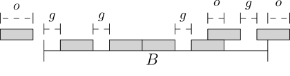
Figure 1: Illustrating gaps (denoted by $g$) and overlaps (denoted by $o$).

A gap refers to a maximal sub-segment of $B$ such that each point of the sub-segment is not covered by any sensors (e.g., see Fig. 1). Each endpoint of any gap is an endpoint of either an sc-interval or $B$. Specifically, consider two adjacent sensors $s_{i}$ and $s_{i+1}$ such that $x_{i}+z<x_{i+1}-z$. If $0\leq x_{i}+z$ and $x_{i+1}-z\leq\beta$, then the interval $[x_{i}+z,x_{i+1}-z]$ is on $B$ and defines a gap, and $s_{i}$ and $s_{i+1}$ are called the left and right generators of the gap, respectively. If $x_{i}+z<0<x_{i+1}-z\leq\beta$, then $[0,x_{i+1}-z]$ is a gap and $s_{i+1}$ is the only generator of the gap. Similarly, if $0\leq x_{i}+z<\beta<x_{i+1}-z$, then $[x_{i}+z,\beta]$ is a gap and $s_{i}$ is the only generator. For any gap $g$, we use $|g|$ to denote its length. For simplicity, if a gap $g$ has only one generator $s_{i}$, then the left/right generator of $g$ is $s_{i}$.

To solve the problem MSBC, the essential task is to move the sensors to cover all gaps by eliminating overlaps, defined as follows. Consider two adjacent sensors $s_{i}$ and $s_{i+1}$. The intersection $I(s_{i})\cap I(s_{i+1})\cap B$ defines an overlap if it is not empty (e.g., see Fig. 1), and we call $s_{i}$ and $s_{i+1}$ the left and right generators of the overlap, respectively. Consider any sensor $s_{i}$. If $I(s_{i})$ is not completely on $B$, then the sub-interval of $I(s_{i})$ that is not on $B$ defines an overlap and $s_{i}$ is its only generator (e.g., see Fig. 1). A subtle situation appears when $I(s_{i})\cap I(s_{i+1})$ contains an endpoint of $B$ in its interior. Refer to Fig. 2 as an example, where $0$ is in the interior of $I(s_{i})\cap I(s_{i+1})$ with $I(s_{i})=[a,b]$ and $I(s_{i+1})=[c,d]$. According to our definition, $s_{i}$ and $s_{i+1}$ together define an overlap $[0,b]$; $s_{i}$ itself defines an overlap $[a,0]$; $s_{i+1}$ itself defines an overlap $[c,0]$. However, to avoid some tedious discussions, we consider the union of $[c,0]$ and $[0,b]$ as a single overlap $[c,b]$ defined by $s_{i}$ and $s_{i+1}$ together, but $s_{i}$ still itself defines the overlap $[a,0]$. Symmetrically, if $I(s_{i})\cap I(s_{i+1})$ contains $\beta$ in its interior, then we consider $I(s_{i})\cap I(s_{i+1})$ as a single overlap defined by $s_{i}$ and $s_{i+1}$, and $s_{i+1}$ itself defines an overlap that is the portion of $I(s_{i+1})$ outside $B$.

For any overlap $o$, we use $|o|$ to denote its length. For simplicity, if an overlap $o$ has only one generator $s_{i}$, then the left/right generator of $o$ is $s_{i}$. We should point out that according to our above definition on overlaps, if an overlap has two different generators, then these two generators must be two adjacent sensors (e.g., $s_{i}$ and $s_{i+1}$ for some $i$). In other words, if the sc-intervals of two non-adjacent sensors (e.g., $s_{i}$ and $s_{i+2}$) intersect, their intersection does not define any overlap.

Clearly, the total number of overlaps and gaps is $O(n)$.

Figure 2: $I(s_{i})\cap I(s_{i+1})$ contains $0$ in its interior. In this case, we consider $s_{i}$ and $s_{i+1}$ together defining an overlap $[c,b]$ and $s_{i}$ itself defining an overlap $[a,0]$.

To solve MSBC, the goal is to move the sensors to cover all gaps by eliminating overlaps. We say a gap/overlap $go_{1}$ is to the left (resp., right) of another gap/overlap $go_{2}$ if the left generator of $go_{1}$ is to the left (resp., right) of the left generator of $go_{2}$ (in the case of Fig. 2, where overlaps $[c,b]$ and $[a,0]$ have the same left generator $s_{i}$, $[a,0]$ is considered to the left of $[c,b]$).

For any two indices $i$ and $j$ with $i\leq j$, let $S(i,j)=\{s_{i},s_{i+1},\ldots,s_{j}\}$.

Below we sketch the $O(n^{2})$ time algorithm in [8] on the containing case where every sc-interval intersects $B$. The algorithm “greedily” covers all gaps from left to right one by one. Suppose the first $i-1$ gaps have just been covered completely and the algorithm is about to cover the gap $g_{i}$.

Let $o_{i}^{r}$ (resp., $o_{i}^{l}$) be the closest overlap to the right (resp., left) of $g_{i}$. We will cover $g_{i}$ by using either $o_{i}^{r}$ or $o_{i}^{l}$. To determine using which overlap to cover $g_{i}$, the costs $C(o_{i}^{r})$ and $C(o_{i}^{l})$ are defined as follows. Let $S_{r}(g_{i})$ be the set of sensors between the right generator of $g_{i}$ and the left generator of $o_{i}^{r}$. Define $C(o_{i}^{r})$ to be $|S_{r}(g_{i})|$. The intuition of this definition is that suppose we shift all sensors of $S_{r}(g_{i})$ to the left for an infinitesimal distance $\epsilon>0$ (such that the gap $g_{i}$ becomes $\epsilon$ shorter), then the sum of the moving distances of all sensors of $S_{r}(g_{i})$ is $\epsilon\cdot C(o_{i}^{r})$. As will be clear later, the current displacement of each sensor in $S_{r}(g_{i})$ may be positive but cannot be negative. For $C(o_{i}^{l})$, it is defined in a slightly different way. Let $S_{l}(g_{i})$ be the set of sensors between the left generator of $g_{i}$ and the right generator of $o_{i}^{l}$, and let $S_{l}^{\prime}(g_{i})$ be the subset of sensors of $S_{l}(g_{i})$ whose displacements are positive. If we shift all sensors in $S_{l}(g_{i})$ to the right for an infinitesimal distance $\epsilon>0$, although the sum of the moving distances of all sensors of $S_{l}(g_{i})$ is $\epsilon\cdot|S_{l}(g_{i})|$, the total moving distance contributed to the sum of the moving distances of all sensors of $S$ is actually $\epsilon\cdot(|S_{l}(g_{i})|-2\cdot|S^{\prime}_{l}(g_{i})|)$ because the sensors of $S^{\prime}_{l}(g_{i})$ are moved towards their original locations. Hence, the cost $C(o_{i}^{l})$ is defined to be $|S_{l}(g_{i})|-2\cdot|S^{\prime}_{l}(g_{i})|$. Note that the sensors in $S_{r}(g_{i})$ or $S_{l}(g_{i})$ are consecutive in their index order.

If $C(o_{i}^{r})<C(o_{i}^{l})$, we move each sensor in $S_{r}(g_{i})$ leftwards by distance $\min\{|o_{i}^{r}|,|g_{i}|\}$, and we call this a left-shift process. Note that if there is any gap $g_{j}$ between two sensors in $S_{r}(g_{i})$, then the above shift process will move $g_{j}$ leftwards as well, but the size and the generators of $g_{j}$ do not change, and thus in the later algorithm we can still use $g_{j}$ without causing any problems. If $|g_{i}|\leq|o_{i}^{r}|$, then after the left-shift process $g_{i}$ is covered completely and we proceed on the next gap $g_{i+1}$. Otherwise, $o_{i}^{r}$ is eliminated and $g_{i}$ is only partially covered. We proceed on the remaining $g_{i}$.

If $C(o_{i}^{r})\geq C(o_{i}^{l})$, we move each sensor in $S_{l}(g_{i})$ rightwards by distance $\min\{|o_{i}^{l}|,|g_{i}|,\alpha\}$, where $\alpha$ is the smallest displacement of the sensors in $S_{l}^{\prime}(g_{i})$, and we call this a right-shift process. If $\alpha$ is the smallest among the three values, then the process makes the displacement of at least one sensor in $S^{\prime}_{l}(g_{i})$ become zero and we call the process as a positive-displacement-removal right-shift process (or PDR process for short). After the process, if $g_{i}$ is only partially covered, we proceed on the remaining $g_{i}$; otherwise we proceed on the next gap $g_{i+1}$.

The algorithm finishes after all gaps are covered. To analyze the running time, there are $O(n)$ shift processes in total. To see this, each shift process covers a gap completely, or eliminates an overlap, or is a PDR process. An observation is that if the displacement of a sensor $s_{i}$ was positive but is made to zero during a PDR process, then the displacement of $s_{i}$ will never become positive again because all uncovered gaps are to the right of $s_{i}$. Therefore, the number of PDR processes is at most $n$. Since the number of gaps and overlaps is $O(n)$, the total number of shift processes in the algorithm is $O(n)$. Each shift process can be done in $O(n)$ time, and thus the algorithm runs in $O(n^{2})$ time.

3 The Containing Case

In this section, we present our algorithm that solves the containing case of MSBC in $O(n\log n)$ time. The high-level scheme of our algorithm is the same as the $O(n^{2})$ time algorithm [8] described in Section 2, but we design efficient data structures such that each shift process can be implemented in $O(\log n)$ amortized time. More specifically, our algorithm maintains an overlap tree $T_{o}$, a position tree $T_{p}$, a left-shift tree $T_{l}$, and a global variable $\gamma$.

3.1 The Overlap Tree $T_{o}$

We store each gap/overlap by recording its generators. Consider any gap $g_{i}$ (which may have been partially covered previously). Our algorithm needs to compute the two overlaps $o_{i}^{l}$ and $o_{i}^{r}$. To this end, we maintain all overlaps in a balanced binary search tree $T_{o}$, called overlap tree, using the indices of the left generators of the overlaps as “keys”. We can find the two overlaps $o_{i}^{l}$ and $o_{i}^{r}$ in $O(\log n)$ time by searching $T_{o}$ with the index of the left generator of $g_{i}$. The tree $T_{o}$ can also support each deletion of any overlap in $O(\log n)$ time if the overlap is eliminated.

Furthermore, $T_{o}$ can help us to compute the costs $C(o_{i}^{l})$ and $C(o_{i}^{r})$ in the following way. After $o_{i}^{r}$ is found, we have $|S_{i}^{r}|=a-b+1$, where $a$ is the index of the left generator of $o_{i}^{r}$ and $b$ is the index of the right generator of $g_{i}$. Hence, $C(o_{i}^{r})=|S_{r}(g_{i})|$ can be computed in $O(\log n)$ time. Similarly, we can obtain $|S_{l}(g_{i})|$. However, to compute $C(o_{i}^{l})$, we also need to know the size $|S^{\prime}_{l}(g_{i})|$, which will be discussed later.

3.2 The Position Tree $T_{p}$

Recall that the algorithm needs to do the left or right shift processes, each of which moves a sequence of consecutive sensors by the same distance. To achieve the overall $O(n\log n)$ time for the algorithm, we cannot explicitly move the involved sensors for each shift process. Instead, we use the following position tree $T_{p}$ to perform each shift implicitly in $O(\log n)$ time.

The tree $T_{p}$ is a complete binary tree of $n$ leaves and $O(\log n)$ height. The leaves from left to right correspond to the sensors in their index order. For each $1\leq j\leq n$, leaf $j$ (i.e., the $j$-th leaf from the left) stores the original location $x_{j}$ of sensor $s_{j}$. Each node of $T_{p}$ (either an internal node or a leaf) is associated with a shift value. Initially the shift values of all nodes of $T_{p}$ are zero. At any moment during the algorithm, the actual location of each sensor $s_{j}$ is $x_{j}$ plus the sum of the shift values of the nodes in the path from the root to leaf $j$ (actually this sum of shift values is exactly the negative value of the current displacement of $s_{j}$), which can be obtained in $O(\log n)$ time.

Now suppose we want to do a right-shift process that moves a sequence of sensors in $S(j,k)$ for $j\leq k$ rightwards by a distance $\delta$. We first find a set $V_{jk}$ of $O(\log n)$ nodes of $T_{p}$ such that the leaves of the subtrees of all these nodes correspond to exactly the sensors in $S(j,k)$. Specifically, $V_{jk}$ is defined as follows. Let $w$ be the lowest common ancestor of leaves $i$ and $j$. Let $\pi^{\prime}_{j}$ be the path from the parent of leaf $j$ to $w$. For each node $v$ in $\pi^{\prime}_{j}$, if the right child of $v$ is not in $\pi^{\prime}_{j}$, then the right child of $v$ is in $V_{jk}$. Leaf $j$ is also in $V_{jk}$. The rest of the nodes of $V_{jk}$ are defined in a symmetric way on the path from the parent of leaf $k$ to $w$. The set $V_{jk}$ can be easily found in $O(\log n)$ time by following the two paths from the root to leaf $j$ and leaf $k$. For each node in $V_{jk}$, we increase its shift value by $\delta$. This finishes the right-shift process, which can be done in $O(\log n)$ time. Similarly, each left-shift process can also be done in $O(\log n)$ time.

After the algorithm finishes, we can use $T_{p}$ to obtain the locations for all sensors in $O(n\log n)$ time.

3.3 The Left-Shift Tree $T_{l}$ and the Global Variable $\gamma$

It remains to compute the size $|S^{\prime}_{l}(g_{i})|$ and the smallest displacement of the sensors in $S^{\prime}_{l}(g_{i})$. Our goal is to compute them in $O(\log n)$ time. This is one main difficulty in our containing case algorithm. We propose a left-shift tree $T_{l}$ to maintain the displacement information of the sensors that have positive displacements (i.e., their current positions are to the left of their original locations).

The tree $T_{l}$ is a complete binary tree of $n$ leaves and $O(\log n)$ height. The leaves from left to right correspond to the $n$ sensors. For each leaf $j$, denote by $\pi_{j}$ the path in $T_{l}$ from the root to the leaf. Each node $v$ of $T_{l}$ is associated with the following information.

1. If $v$ is a leaf, then $v$ is associated with a flag, and $v.flag$ is set to “valid” if the current displacement of $s_{i}$ is positive and “invalid” otherwise. Initially all leaves are invalid. If the flag of leaf $j$ is valid/invalid, we also say the sensor $s_{j}$ is valid/invalid. Thus, $S^{\prime}_{l}(g_{i})$ is the set of valid sensors of $S_{l}(g_{i})$.

2. As in the position tree $T_{p}$, regardless of whether $v$ is an internal node or a leaf, $v$ maintains a shift value $v.shift$. At any moment during the algorithm, for each leaf $j$, the sum of all shift values of the nodes in the path $\pi_{j}$ is exactly the negative value of the current displacement of the sensor $s_{j}$.

3. Node $v$ maintains a min value $v.min$, which is equal to $d$ minus the sum of the shift values of the nodes in the path from $v$ to the root, where $d$ is the smallest displacement among all valid leaves in the subtree rooted at $v$, and further, the index of the corresponding sensor that has the above smallest displacement $d$ is also maintained in $v$ as $v.index$.

   If no leaves in the subtree of $V$ are valid, then $v.min=+\infty$ and $v.index=0$.

4. Node $v$ maintains a num value $v.num$, which is the number of valid leaves in the subtree of $v$. Initially $v.num=0$ for all nodes.

The tree $T_{l}$ can support the following operations in $O(\log n)$ time each.

set-valid

Given a sensor $s_{j}$, the goal of this operation is to set the flag of the $j$-th leaf valid.

To perform this operation, we first find the leaf $j$, denoted by $u$. We set $u.flag=valid$, $u.min=0$, $u.index=j$. Next, we update the min and index values of the other nodes in the path $\pi_{j}$ in a bottom-up manner. Beginning from the parent of $u$, for each node $v$ in $\pi_{j}$, we set $v.min=\min\{v_{l}.min+v_{l}.shift,v_{r}.min+v_{r}.shift\}$ where $v_{l}$ and $v_{r}$ are the left and right child of $v$, respectively, and we set $v.index$ to $v_{l}.index$ if $v_{l}$ gives the above minimum value and $v_{r}.index$ otherwise.

Finally, we update the num values for all nodes in the path $\pi_{j}$ by increasing $v.num$ by one for each node $v\in\pi_{j}$.

Hence, the set-valid operation can be done in $O(\log n)$ time.

set-invalid

Given a sensor $s_{j}$, the goal of this operation is to set the flag of the $j$-th leaf invalid.

We first find leaf $j$, set it invalid, set its min value to $+\infty$, and set its num value to $0$. Then, we update the min, index, and num values of the nodes in the path $\pi_{j}$ similarly as in the above set-valid operation. We omit the details. The set-invalid operation can be done in $O(\log n)$ time.

left-shift

Given two indices $j$ and $k$ with $j\leq k$, as well as a distance $\delta$, the goal of this operation is to move each sensor in $S(j,k)$ leftwards by $\delta$. It is required that $\delta$ is small enough such that any valid (resp., invalid) sensor before the operation is still valid (resp., invalid) after the operation.

The operation can be performed in a similar way as we did on the position tree $T_{p}$, with the difference that we also need to update the shift, min, and index values of some nodes. Specifically, we first compute the set $V_{jk}$ of $O(\log n)$ nodes, as defined in the position tree $T_{p}$, and then for each node $v$ of $V$, we increase its shift value by $\delta$.

Next, we update the min and index values. An easy observation is that only those nodes on the two paths $\pi_{j}$ and $\pi_{k}$ need to have their min and index values updated. Specifically, for $\pi_{j}$, we follow it from leaf $j$ in a bottom-up manner, for each node $v$, we update $v.min$ and $v.index$ in the same way as we did in the set-valid operations. We do the similar things for the path $\pi_{k}$. The time for performing this operation is $O(\log n)$.

right-shift

Given two indices $j$ and $k$ with $j\leq k$, as well as a distance $\delta$, the goal of this operation is to move each sensor in $S(j,k)$ rightwards by $\delta$. Similarly, $\delta$ is small enough such that any valid (resp., invalid) sensor before the operation is still valid (resp., invalid) after the operation.

This operation can be performed in a symmetric way as the above left-shift operation and we omit the details.

find-min

Given two indices $j$ and $k$ with $j\leq k$, the goal is to find the smallest displacement and the corresponding sensor among all valid sensors in $S(j,k)$.

We first find the set $V_{jk}$ of $O(\log n)$ nodes as before. For each node $v\in V_{jk}$, we compute the smallest displacement among all valid nodes in its subtree, which is equal to $v.min$ plus the shift values of the nodes in the path from $v$ to the root. These smallest displacements for all nodes in $V_{jk}$ can be computed in $O(\log n)$ time in total by traversing the two paths $\pi_{j}$ and $\pi_{k}$ in the top-down manner. The smallest displacement among all valid sensors in $S(j,k)$ is the minimum among all above $O(\log n)$ smallest displacements, and the corresponding sensor for the smallest displacement can be immediately obtained by using $v.index$ associated with each node of $V_{jk}$. Thus, each find-min operation can be done in $O(\log n)$ time.

find-num

Given two indices $j$ and $k$ with $j\leq k$, the goal is to find the number of valid sensors in $S(j,k)$.

We first find the set $V_{jk}$ of $O(\log n)$ nodes as before, and then return the sum of the values $v.num$ for all nodes $v\in V_{jk}$. Hence, $O(\log n)$ time is sufficient for performing the operation.

In addition, our algorithm maintains a global variable $\gamma$ that is the rightmost sensor that has ever been moved to the left. We will use $\gamma$ to determine whether we should do a set-valid operation on a sensor in the left-shift tree $T_{l}$ and make sure the total number of set-valid operations on $T_{l}$ in the entire algorithm is at most $n$. Initially, $\gamma=0$. As will be clear later, the variable $\gamma$ will never decrease during the algorithm.

3.4 The $O(n\log n)$ Time Algorithm

Using the three trees $T_{o}$, $T_{p}$, $T_{l}$, and the global variable $\gamma$, we implement the algorithm [8] described in Section 2 in $O(n\log n)$ time, as follows.

The initialization of these trees can be easily done in $O(n\log n)$ time. Suppose the algorithm is about to consider gap $g_{i}$. We assume the three trees and $\gamma$ have been correctly maintained. We first use use the overlap tree $T_{o}$ to find the two overlaps $o_{i}^{r}$ and $o_{i}^{l}$ in $O(\log n)$ time, as discussed earlier. The two numbers $|S_{l}(g_{i})|$ and $|S_{r}(g_{i})|$, as well as the cost $C(o_{i}^{r})$, are also determined. Next, we find $|S^{\prime}_{l}(g_{i})|$ by doing a find-num operation on $T_{l}$ using the index of the right generator of $o_{i}^{l}$ and the index of the left generator of $g_{i}$. The cost $C(o_{i}^{r})$ is thus obtained. Depending on whether $C(o_{i}^{r})<C(o_{i}^{l})$, we have two main cases.

3.4.1 Case $C(o_{i}^{r})<C(o_{i}^{l})$

If $C(o_{i}^{r})<C(o_{i}^{l})$, we do a left-shift process that moves all sensors in $S_{r}(g_{i})$ leftwards by distance $\delta=\min\{|g_{i}|,|o_{i}^{r}|\}$. Note that $S_{r}(g_{i})=S(j,k)$ with $j$ being the index of the right generator of $g_{i}$ and $k$ being the index of the left generator of $o_{i}^{r}$. To implement the above left-shift process, we first do a left shift on the position tree $T_{p}$, as described earlier. Then, we update the left-shift tree $T_{l}$ and the variable $\gamma$ in the following way.

Since $o_{i}^{r}$ is an overlap and the gaps that have been covered are all to the left of $o_{i}^{r}$, no sensor to the right of $o_{i}^{r}$ has ever been moved. Specifically, sensor $s_{t}$ has never been moved, for any $t>k$. This implies that $\gamma\leq k$.

If $\gamma<j$, then for each sensor $s_{t}$ with $j\leq t\leq k$, we first do a set-valid operation on $T_{l}$ on $s_{t}$ and then do a left-shift operation on $T_{l}$ on $s_{t}$ with distance $\delta$.

If $j\leq\gamma<k$, we have the following lemma.

Lemma 1

If $j\leq\gamma<k$, then right before the above left-shift process, all sensors in $S(j,\gamma)$ have positive displacements and thus are valid.

Proof: We consider the situation right before the above left-shift process.

First of all, we claim that the displacement of $s_{\gamma}$ must be positive. Indeed, according to the definition of $\gamma$, if the displacement of $s_{\gamma}$ is not positive, then there must be a shift process previously in the algorithm that moved $s_{\gamma}$ rightwards. However, since the gaps that have been considered by the algorithm are all to the left of $g_{i}$ and thus to the left of $s_{\gamma}$, $s_{\gamma}$ never had any chance to be moved rightwards. The claim thus follows. Hence, if $j=\gamma$, the lemma is trivially true.

If $j<\gamma$, assume to the contrary that there is a sensor $s_{t}$ with $j\leq t<\gamma$ whose displacement is not positive. Since the displacement of $s_{\gamma}$ is positive, the above situation can only happen if the algorithm covered a gap between $s_{t}$ and $s_{\gamma}$, which contradicts with the fact that all gaps that have been covered by the algorithm are to the left of $g_{i}$ and thus to the left of $s_{j}$. Thus, the lemma follows. $\Box$

If $j\leq\gamma<k$, for each $t$ with $\gamma<t\leq k$, we first do a set-valid operation on $s_{t}$ and then do a left-shift operation on $s_{t}$ with distance $\delta$ in $T_{l}$. Finally, we do a left-shift operation for the sensors in $S(j,\gamma)$ on $T_{l}$ with distance $\delta$. Based on Lemma 1, the tree $T_{l}$ is now correctly updated.

Note that during the above left-shift process, we did multiple set-valid operations and each of them is followed immediately by a left-shift operation. An observation is that the total number of set-valid operations in the entire algorithm is at most $n$, because the sensors that are set to valid during this left-shift processes have never been set to valid before as their indices are larger than $\gamma$. The number of left-shift operations immediately following these set-valid operations is thus also at most $n$.

Finally, we update $\gamma$ to $k$.

If $|g_{i}|<|o_{i}^{r}|$, we proceed on the next gap $g_{i+1}$. Otherwise, $o_{i}^{r}$ is eliminated and we delete it from the overlap tree $T_{o}$. Since $g_{i}$ is only partially covered, we proceed on the remaining $g_{i}$ with the same approach (in the special case $|g_{i}|=|o_{i}^{r}|$, we proceed on $g_{i+1}$).

3.4.2 Case $C(o_{i}^{r})\geq C(o_{i}^{l})$

If $C(o_{i}^{r})\geq C(o_{i}^{l})$, we perform a right-shift process that moves all sensors in $S_{l}(g_{i})$ rightwards by distance $\delta=\min\{|g_{i}|,|o_{i}^{l}|,\alpha\}$, where $\alpha$ is the smallest displacement of the sensors in $S^{\prime}_{l}(g_{i})$. Let $j$ be the index of the right generator of $o_{i}^{l}$ and $k$ be the index of the left generator of $g_{i}$. Hence, $S_{l}(g_{i})=S(j,k)$.

To implement the right-shift process, we first do a find-min operation on $T_{l}$ with indices $j$ and $k$ to compute $\alpha$. Then, we update the position tree $T_{p}$ by doing a right-shift operation for the sensors in $S(j,k)$ with distance $\delta$. Since no sensor is moved leftwards in the above process, we do not need to update $\gamma$.

Next, we update the other two trees $T_{o}$ and $T_{l}$, depending on which of the three values $|g_{i}|$, $|o_{i}^{l}|$, and $\alpha$ is the smallest.

If $\delta=\alpha$, we do a right-shift operation with indices $j$ and $k$ for distance $\delta=\alpha$ on $T_{l}$. Recall that the find-min operation can also return the sensor that gives the sought smallest displacement. Suppose the above find-min operation on $T_{l}$ returns $s_{t}$ whose displacement is $\alpha$, with $j\leq t\leq k$. Since the displacement of $s_{t}$ now becomes zero, we do a set-invalid operation on $s_{t}$ in $T_{l}$. Note that although it is possible that $\gamma=t$, we do not need to update $\gamma$.

We should point out a subtle situation where multiple sensors in $S^{\prime}_{l}(g_{i})$ had displacements equal to $\alpha$. For handling this case, we do another find-min operation on $T_{l}$ with indices $j$ and $k$. If the smallest displacement found by the operation is zero, then we do the set-invalid operation on $T_{l}$ on the sensor returned by this find-min operation. We keep doing the find-min operations until the smallest displacement found above is larger than zero. Although there may be multiple set-invalid and find-min operations during the above procedure, the total number of these operations is $O(n)$ in the entire algorithm. To see this, it is sufficient to show that the number of set-invalid operations is $O(n)$ because there is exactly one find-min operation following each set-invalid operation. After each set-invalid operation, say, on a sensor $s_{t}$, we claim that the sensor $s_{t}$ will never be set to valid again in the algorithm. Indeed, since the displacement of $s_{t}$ was positive, according to the definition of $\gamma$, we have $t\leq\gamma$. Since each set-valid operation is only on sensors with indices larger than $\gamma$ and the value $\gamma$ never decreases, $s_{t}$ will never be set to valid again in the algorithm. In fact, $s_{t}$ will never be moved leftwards in the algorithm because $s_{t}$ is to the left $g_{i}$ and all gaps that will be covered in the algorithm are to the right of $g_{i}$ and thus are to the right of $s_{t}$.

This finishes the discussion for the case $\alpha=\delta$. Below we assume $\delta<\alpha$.

We do the right-shift operation with indices $j$ and $k$ for distance $\delta$ on $T_{l}$. Since $\delta<\alpha$, no valid sensor in $S^{\prime}_{l}(g_{i})$ will become invalid due to the right-shift. If $\delta=|o_{i}^{l}|$, we delete $|o_{i}^{l}|$ from $T_{o}$ since $o_{i}^{l}$ is eliminated. If $\delta=|g_{i}|$, we proceed on the next gap $g_{i+1}$; otherwise, we proceed on the remaining $g_{i}$.

The algorithm finishes after all gaps are covered. The above discussion also shows that the running time of the algorithm is bounded by $O(n\log n)$.

4 The One-Sided Case

In this section, we solve the one-sided case in $O(n\log n)$ time, by using our algorithm for the containing case in Section 3 as an initial step. In the one-sided case, the sensors whose covering intervals do not intersect $B$ are all in one side of $B$, and without loss of generality, we assume it is the right side. Specifically, we assume $0\leq x_{1}+z$ holds. We assume at least one sc-interval does not intersect $B$ since otherwise it would become the containing case. Note that this implies $\beta<x_{n}-z$.

We use configuration to refer to a specification of where each sensor is located. For example, in the input configuration, each sensor $s_{i}$ is located at $x_{i}$.

A sequence of consecutive sensors $s_{i},s_{i+1},\ldots s_{j}$ are said to be in attached positions if for each $i\leq k\leq j-1$ the right endpoint of the covering interval $I(s_{k})$ of $s_{k}$ is at the same position as the left endpoint of $I(s_{k+1})$.

4.1 Observations

First, we show in the following lemma that a special case where no sc-interval intersects $B$, i.e., $\beta<x_{1}-z$, can be easily solved in $O(n)$ time.

Lemma 2

If $\beta<x_{1}-z$, we can find an optimal solution in $O(n)$ time.

Proof: If $\beta<x_{1}-z$, then all sensor covering intervals are strictly to the right side of $B$. According to the order preserving property, in the optimal solution $I(s_{1})$ must have its left endpoint at $0$ (i.e., $s_{1}$ is at $z$). Note that we need at least $\lceil\frac{\beta}{2z}\rceil$ sensors to fully cover $B$. Since all sensors have their covering intervals strictly to the right side of $B$ and no sensor intersects $B$, in the optimal solution sensors in $S(1,\lceil\frac{\beta}{2z}\rceil)$ must be in attached positions. Therefore, the optimal solution has a very special pattern: $s_{1}$ is at $z$, sensors in $S(1,\lceil\frac{\beta}{2z}\rceil)$ are in attached positions, and other sensors are at their original locations. Hence, we can compute this optimal solution in $O(n)$ time. $\Box$

In the following, we assume $\beta\geq x_{1}-z$, i.e., $I(s_{1})$ intersects $B$. Let $m$ be the largest index such that $I(s_{m})$ intersects $B$. Note that $m<n$ due to $\beta<x_{n}-z$. To simplify the notation, let $S_{I}=S(1,m)$ and $S_{R}=S(m+1,n)$.

Our containing case algorithm is not applicable here and one can easily verify that the cost function we used in the containing case do not work for the sensors in $S_{R}$. More specifically, suppose we want to move a sensor $s_{i}$ in $S_{R}$ leftwards to cover a gap; there will be an “additive” cost $x_{i}-z-\beta$, i.e., $I(s_{i})$ has to move leftwards by that distance before it touches $B$. Recall that the cost we defined on overlaps in the containing case is a “multiplicative” cost, and the above additive cost is not consistent with the multiplicative cost. To overcome this difficulty, we have to use a different approach to solve the one-sided case.

Our main idea is to somehow transform the one-sided case to the containing case so that we can use our containing case algorithm. Let $D_{opt}$ be any optimal solution for our problem. By slightly abusing notation, depending on the context, a “solution” may either refer to the configuration of the solution or the sum of moving distances of all sensors in the solution. If no sensor of $S_{R}$ is moved in $D_{opt}$, then we can compute $D_{opt}$ by running our containing case algorithm on the sensors in $S_{I}$. Otherwise, let $m^{*}$ be the largest index such that sensor $s_{m^{*}}\in S_{R}$ is moved in $D_{opt}$. If we know $m^{*}$, then we can easily compute $D_{opt}$ in $O(n\log n)$ time as follows. First, we “manually” move all sensors in $S(m+1,m^{*})$ leftwards to $\beta+z$ such that the left endpoints of their covering intervals are at $\beta$. Then, we apply our containing case algorithm on all sensors in $S_{1m^{*}}$, which now all have their covering intervals intersecting $B$ (which is an instance of the containing case), and let $D(m^{*})$ be the solution obtained above. Based on the order preserving property, the following lemma shows that $D(m^{*})$ is $D_{opt}$.

Lemma 3

$D(m^{*})$ is $D_{opt}$.

Proof: Since $s_{m^{*}}$ is moved in $D_{opt}$, $I(s_{m^{*}})$ must intersect $B$ in $D_{opt}$. Based on the order preserving property, for each $m+1\leq i\leq m^{*}$, $I(s_{i})$ intersects $B$ in $D_{opt}$, which implies that the location of $s_{i}$ in $D_{opt}$ must be to the left of $\beta+z$. On the other hand, since no sensor $s_{i}$ with $i>m^{*}$ is moved, sensors in $S(m^{*}+1,n)$ are useless for computing $D_{opt}$. Therefore, $D_{opt}$ is essentially the optimal solution for the containing case on $S(1,m^{*})$ after each sensor in $S(m+1,m^{*})$ is moved leftwards to $\beta+z$, i.e., $D_{opt}=D(m^{*})$. The lemma thus follows. $\Box$

By the above discussion, one main task of our algorithm is to determine $m^{*}$.

For each $j$ with $m<j\leq n$, let $D_{s}(j)=\sum_{i=m+1}^{j}(x_{i}-z-\beta)$, i.e., the sum of the moving distances for “manually” moving all sensors in $S(m+1,j)$ leftwards to $\beta+z$, and we use $F_{j}$ to denote the configuration after the above manual movement and we let $F_{j}$ contain only the sensors in $S(1,j)$ (i.e., sensors in $S(j+1,n)$ do not exist in $F_{j}$). Let $D_{s}(m)=0$ and $F_{m}$ be the input configuration but containing only sensors in $S(1,m)$. For each $m\leq j\leq n$, suppose we apply our containing case algorithm on $F_{j}$ and denote by $D_{c}(j)$ the solution (in the case where $\beta>2zj$, we let $D_{c}(j)=+\infty$), and further, let $D(j)=D_{s}(j)+D_{c}(j)$.

The above discussion leads to the following lemma.

Lemma 4

$D_{opt}=\min_{m\leq j\leq n}D(j)$ and $m^{*}=\operatorname*{arg\,min}_{m\leq j\leq n}D(j)$.

4.2 The Algorithm Description and Correctness

Lemma 4 leads to a straightforward $O(n^{2}\log n)$ time algorithm for the one-sided case, by computing $D(j)$ in $O(n\log n)$ time for each $j$ with $m\leq j\leq n$, as suggested above. In the sequel, by exploring the solution structures, we present an $O(n\log n)$ time solution. The algorithm itself is simple, but it is not trivial to discover the observations behind the scene.

Our algorithm will compute $D(j)$ for all $j=m,m+1,\ldots,n$. Recall that $D(j)=D_{s}(j)+D_{c}(j)$. Since it is easy to compute all $D_{s}(j)$’s in $O(n)$ time, we focus on computing $D_{c}(j)$’s. The main idea is the following. Suppose we already have the solution $D_{c}(j-1)$, which can be considered as being obtained by our containing case algorithm. To compute $D_{c}(j)$, since we have an additional overlap defined by $s_{j}$ at $\beta+z$, i.e., the sc-interval $I(s_{j})$, we modify $D_{c}(j-1)$ by “reversing” some shift processes that have been performed in the containing algorithm when computing $D_{c}(j-1)$, i.e., using $I(s_{j})$ to cover some gaps that were covered by other overlaps in $D_{c}(j-1)$. The details are given below.

We first compute $D_{c}(m)$ on the configuration $F_{m}$. If $2zm<\beta$, then $D_{c}(j)=+\infty$ for each $m\leq j<\lceil\frac{\beta}{2z}\rceil$; in this case, we can start from computing $D_{c}(\lceil\frac{\beta}{2z}\rceil)$ and use the similar idea as the following algorithm. To make it more general, we assume $m\geq\lceil\frac{\beta}{2z}\rceil$, and thus $D_{c}(m)<+\infty$.

Consider our containing case algorithm for computing $D_{c}(m)$. Recall that our containing case algorithm consists of shift processes and each shift process covers a gap using an overlap. Let $p_{1},p_{2},\ldots,p_{q}$ be the shift processes performed in the algorithm in the inverse order of time (e.g., $p_{1}$ is the last process), where $q$ is the total number of processes in the algorithm. For each $1\leq i\leq q$, let $g_{i}$ be the gap covered in the process $p_{i}$ by using/eliminating an overlap, denoted by $o_{i}$. Note that each gap/overlap above may not be an original gap/overlap in the input configuration but only a subset of an original gap/overlap. It holds that $|o_{i}|=|g_{i}|$ for each $1\leq i\leq q$. We call $G=\{g_{1},g_{2},\ldots,g_{q}\}$ the gap list of $D_{c}(m)$. For each $i$, we use $C(o_{i})$ to denote the cost of $o_{i}$ when the algorithm uses $o_{i}$ to cover $g_{i}$ in the process $p_{i}$. Note that the above process information can be explicitly stored during our containing case algorithm without affecting the overall running time asymptotically. We will use these information later. Note that according to our algorithm the gaps in $G$ are sorted from right to left.

Next, we compute $D_{c}(m+1)$, by modifying the configuration $D_{c}(m)$. Comparing with $F_{m}$, the configuration $F_{m+1}$ has an additional overlap defined by $s_{m+1}$ at $\beta+z$, and we use $o(s_{m+1})$ to denote it. We have the following lemma.

Lemma 5

$D_{c}(m+1)=D_{c}(m)$ holds if one of the following happens: (1) the coordinate of the right endpoint of $I(s_{m})$ is strictly larger than $\beta$; (2) $o_{1}$ is to the right of $g_{1}$; (3) $o_{1}$ is to the left of $g_{1}$ and the cost $C(o_{1})$ is not greater than the number of sensors between $g_{1}$ and $s_{m+1}$.

Proof: We prove Case (3) first.

Suppose that we run our containing case algorithm on both $F_{m}$ and $F_{m+1}$ simultaneously. We use $A_{m}$ to denote the algorithm on $F_{m}$ and use $A_{m+1}$ to denote the algorithm on $F_{m+1}$. Below we will show that every shift process of $A_{m}$ and $A_{m+1}$ is exactly the same, which proves $D_{c}(m+1)=D_{c}(m)$.

Consider any shift process $p_{j}$. We assume the processes before $p_{j}$ on both algorithms are the same, which holds for $j=q$. In $A_{m}$, the process covers gap $g_{j}$ by using overlap $o_{j}$.

If $o_{j}$ is to the right of $g_{j}$, then since $o(s_{m+1})$ is the rightmost overlap in $F_{m+1}$, algorithm $A_{m+1}$ also uses $o_{j}$ to cover $g_{j}$, which is the same as $A_{m}$.

If $o_{j}$ is to the left of $g_{j}$, then depending on whether $o(s_{m+1})$ is the only overlap to the right of $g_{j}$, there are two cases.

1. If $o(s_{m+1})$ is not the only overlap to the right $g_{j}$, then let $o$ be the closest overlap to $g_{j}$ among the overlaps to the right of $g_{j}$. According to our containing algorithm, the current process of the algorithm only depends on the costs of the two overlaps $o_{j}$ and $o$. Hence, algorithm $A_{m+1}$ uses the same shift process to cover $g_{j}$ as that in $A_{m}$, i.e, use $o_{j}$ to cover $g_{j}$.

2. If $o(s_{m+1})$ is the only overlap to the right $g_{j}$, then the current process of algorithm $A_{m+1}$ depends on the costs of the two overlaps $o_{j}$ and $o(s_{m+1})$. In the following, we show that $C(o_{j})\leq C(o(s_{m+1}))$, and thus algorithm $A_{m+1}$ also uses $o_{j}$ to cover $g_{j}$, as in $A_{m}$.

   Recall that the list of gaps $g_{1},g_{2},\ldots,g_{q}$ are sorted from right to left by their generators. Thus, the gaps $g_{j},g_{j-1},\ldots,g_{1}$ are sorted from left to right. Since $o(s_{m+1})$ is the only overlap to the right $g_{j}$ in $A_{m+1}$, there is no overlap in $A_{m}$ to the right of $g_{t}$ for any $t$ with $j\geq t\geq 1$. Hence, algorithm $A_{m}$ will have to uses the overlaps to the left of $g_{t}$ to cover $g_{t}$ for each $t$ with $j\geq t\geq 1$. In other words, all overlaps $o_{j},o_{j-1},\ldots,o_{1}$ are to the left of all gaps $g_{j},g_{j-1},\ldots,g_{1}$, which implies that the above list of overlaps are sorted from right to left and $C(o_{j})\leq C(o_{j-1})\leq\cdots\leq C(o_{1})$.

   Since $g_{1}$ is to the right of $g_{j}$, the cost $C(o(s_{m+1}))$, which is the number of sensors between $g_{j}$ and $s_{m+1}$, is no less than the number of sensors between $g_{1}$ and $s_{m+1}$. Since in Case (3) the number of sensors between $g_{1}$ and $s_{m+1}$ are at least $C(o_{1})$, we obtain that $C(o(s_{m+1}))\geq C(o_{1})\geq C(o_{j})$.

The above shows that every shift process of $A_{m}$ and $A_{m+1}$ is the same, which proves that $D_{c}(m+1)=D_{c}(m)$ holds for Case (3).

The proofs of the first two cases are similar to the above, and we only sketch them below.

Case (1) means that sensor $s_{m}$ still defines an overlap, say $o$, to the right of $B$. If we run our containing case algorithm on $F_{m+1}$ to compute $D_{c}(m+1)$, sensor $s_{m+1}$ will not be moved since the overlap $o(s_{m+1})$ is to the right of $o$. Hence, $D_{c}(m+1)=D_{c}(m)$ holds.

Case (2) means the last shift process covers $g_{1}$ using $o_{1}$ that is to the right of $g_{1}$. If we run our containing case algorithm on $F_{m+1}$, overlap $o(s_{m+1})$ will never have any chance to be used to cover any gap, because $o(s_{m+1})$ is the rightmost overlap of $F_{m+1}$. Hence, $D_{c}(m+1)=D_{c}(m)$ holds. $\Box$

To compute $D_{c}(m+1)$, we first check whether one of the three cases in Lemma 5 happens, which can be done in constant time by the above process information stored when computing $D_{c}(m)$. If any of the three cases happens, we are done for computing $D_{c}(m+1)$. Below, we assume none of the cases happens.

Let $C(s_{m+1},g_{1})$ be the number of sensors between $g_{1}$ and $s_{m+1}$, which would be the cost of the overlap $o(s_{m+1})$ if it were there right before we cover $g_{1}$. Note that since we know the generators of $g_{1}$, $C(s_{m+1},g_{1})$ can be computed in constant time (e.g., if $g_{1}$ has two generators, $C(s_{m+1},g_{1})=m+1-a+1$, where $a$ is the index of the right generator of $g_{1}$).

Define $R(g_{1})$ to be $C(s_{m+1},g_{1})-C(o_{1})$. We can consider $R(g_{1})$ as the “unit revenue” (or savings) if we use $o(s_{m+1})$ to cover $g_{1}$ instead of using $o_{1}$. Note that $R(g_{1})>0$ otherwise the third case of Lemma 5 would happen. Hence, it is possible to obtain a better solution than $D_{c}(m)$ by using $o(s_{m+1})$ to cover $g_{1}$ instead of $o_{1}$. Note that $|g_{1}|\leq 2z$ and $|o(s_{m+1})|=2z$.

If $|o(s_{m+1})|=|g_{1}|$, then we use $o(s_{m+1})$ to cover $g_{1}$. Specifically, we move all sensors in $S(a,m+1)$ leftwards by distance $|g_{1}|$, where $a$ is the index of the right generator of the overlap $o_{1}$. The above essentially “restores” the overlap $o_{1}$ and covers $g_{1}$ by eliminating $o(s_{m+1})$. We refer to it as a reverse operation (i.e., it reverses the shift process that covers $g_{1}$ by using $o_{1}$ in the algorithm for computing $D_{c}(m)$). Due to $|o(s_{m+1})|=|g_{1}|$, after the reverse operation, $g_{1}$ is fully covered by $o(s_{m+1})$ and $o(s_{m+1})$ is eliminated. We will show later in Lemma 6 that the current configuration is $D_{c}(m+1)$. Note that $D_{c}(m+1)=D_{c}(m)-R(g_{1})\cdot|g_{1}|$. Again, $o_{1}$ is restored in $D_{c}(m+1)$. Finally, we remove $g_{1}$ from the list $G$.

If $|g_{1}|<|o(s_{m+1})|$, then we do a revere operation by using $o(s_{m+1})$ to cover $g_{1}$ and restore $o_{1}$, after which $o(s_{m+1})$ is not eliminated but becomes shorter. We remove $g_{1}$ from $G$ and proceed on the next gap $g_{2}$.

In general, suppose we have covered gaps $g_{1},g_{2},\ldots,g_{k}$ by using $o(s_{m+1})$ and the overlap $o(s_{m+1})$ still partially remains (i.e., $\sum_{t=1}^{k}|g_{i}|<2z$). The above gaps have all been removed from $G$. Let $F^{\prime}$ denote the current configuration. If $G$ is now empty, then we are done with computing $D_{c}(m+1)$, which is equal to $D_{c}(m)-\sum_{t=1}^{k}R(g_{t})\cdot|g_{t}|$; otherwise, we consider gap $g_{k+1}$, as follows.

Similar to Lemma 5, we will show later in Lemma 6 that $F^{\prime}$ is $D_{c}(m+1)$ if one of the following two cases happens: (1) $o_{k+1}$ is to the right of $g_{k+1}$; (2) $o_{k+1}$ is to the left of $g_{k+1}$ but $C(o_{k+1})$ is not greater than the number of sensors between $g_{k+1}$ and $s_{m+1}$. If one of the above two cases happens, then we are done with computing $D_{c}(m+1)$, which is equal to $D_{c}(m)-\sum_{t=1}^{k}R(g_{t})\cdot|g_{t}|$. Otherwise, we do the following. Note that the length of $o(s_{m+1})$ in $F^{\prime}$ is $2z-\sum_{t=1}^{k}|g_{t}|$. Depending on whether $|o(s_{m+1})|\geq|g_{k+1}|$, there are two cases. As for $g_{1}$, we define $C(s_{m+1},g_{k+1})$ as the number of sensors between $g_{k+1}$ and $s_{m+1}$, and define $R(g_{k+1})=C(o_{k+1})-C(s_{m+1},g_{k+1})$.

1. If $|o(s_{m+1})|\geq|g_{k+1}|$, then we do a reverse operation to cover $g_{k+1}$ by using $o(s_{m+1})$. If $|o(s_{m+1})|=|g_{k+1}|$, we are done with computing $D_{c}(m+1)$, which is equal to $D_{c}(m)-\sum_{t=1}^{k+1}R(g_{t})\cdot|g_{t}|$; otherwise, we proceed on the next gap $g_{k+2}$. In either case, we remove $g_{k+1}$ from $G$, and the reverse operation restores the overlap $o_{k+1}$.

2. If $|o(s_{m+1})|<|g_{k+1}|$, then $o(s_{m+1})$ is not long enough to cover $g_{k+1}$. We do a reverse operation to use $o(s_{m+1})$ to partially cover $g_{k+1}$ of length $|o(s_{m+1})|$, and the remaining part of $g_{k+1}$ is still covered by $o_{k+1}$. We are done with computing $D_{c}(m+1)$, which is equal to $D_{c}(m)-\sum_{t=1}^{k}R(g_{t})\cdot|g_{t}|-R(g_{k+1})\cdot|o(s_{m+1})|$. Since $g_{k+1}$ still partially remains in $D_{c}(m+1)$, we do not remove $g_{k+1}$ from $G$ but change its size accordingly. In addition, overlap $o_{k+1}$ is partially restored in $D_{c}(m+1)$ because its size is $|o(s_{m+1})|$, which is smaller than its original size.

The algorithm stops after $D_{c}(m+1)$ is obtained.

Lemma 6

The solution obtained in the above algorithm is $D_{c}(m+1)$.

Proof: Let $F$ be the configuration obtained by our algorithm. Below we show that $F$ is $D_{c}(m+1)$. If one of the three cases in Lemma 5 happens, then by Lemma 5, $F$ is $D_{c}(m+1)$. Below we assume none of the three cases in Lemma 5 happens.

Suppose that we run our containing case algorithm on both $F_{m}$ and $F_{m+1}$ simultaneously. Let $A_{m}$ be the algorithm on $F_{m}$ and let $A_{m+1}$ be the algorithm on $F_{m+1}$.

Consider any shift process $p_{i}$ of $A_{m}$. We assume the processes before $p_{i}$ on both algorithms are the same, which holds for $i=q$. By the proof of Lemma 5, $p_{i}$ may not be the same in $A_{m}$ and $A_{m+1}$ only if for each process $p_{j}$ after $p_{i}$ (i.e., $j\leq i$ since the order of processes follows the reverse order the time), $o_{j}$ is to the left of $g_{j}$, i.e., $p_{j}$ is a right-shift process. Therefore, we only need to consider the right-shift processes after the last left-shift process in $A_{m}$.

Let $k$ be the smallest index with $0\leq k\leq q-1$ such that $o_{k+1}$ is to the right of $g_{k+1}$, i.e., $p_{1},p_{2},\ldots,p_{k}$ are the right-shift processes after the last left-shift process in $A_{m}$. Note that $k\neq 0$ since otherwise Case (2) of Lemma 5 would happen. Hence, the process $p_{i}$ with $k+1\leq i\leq q$ is the same in both $A_{m}$ and $A_{m+1}$.

Since none of the cases in Lemma 5 happens, $C(o_{1})>C(s_{m+1},g_{1})$. Let $t$ be the largest index such that $C(o_{t})>C(s_{m+1},g_{t})$. For each process $p_{i}$ with $k\leq i\leq t+1$, since $C(o_{i})\leq C(s_{m+1},g_{i})$, the process is the same in both $A_{m}$ and $A_{m+1}$. In summary, the above shows that if $q\geq i\geq t+1$, the process $p_{i}$ is the same in both $A_{m}$ and $A_{m+1}$, i.e., the first $(q-t+1)$ processes in both $A_{m}$ and $A_{m+1}$ are the same.

Consider the next process $p_{t}$, which covers gap $g_{t}$ by using $o_{t}$ in $A_{m}$. In $A_{m+1}$, however, using $o(s_{m+1})$ to cover it can give a better solution. Depending on whether $\sum_{i=1}^{t}|g_{i}|\leq 2z$, there are two cases.

1. If $\sum_{i=1}^{t}|g_{i}|\leq 2z=|o(s_{m+1})|$, then since $o(s_{m+1})$ is long enough, $A_{m+1}$ will use $o(s_{m+1})$ to cover all gaps from $g_{t}$ to $g_{1}$ and thus obtain $D_{c}(m+1)$. Let $s_{h}$ be the left generator of $g_{t}$ and let $x(s_{h})$ be the location of $s_{h}$ in the configuration right after the process $p_{t+1}$. Since the algorithm $A_{m+1}$ uses $o(s_{m+1})$ to cover all gaps from $g_{t}$ to $g_{1}$, the location of $s_{h}$ does not change, which implies that the locations of $s_{h}$ in both $D_{c}(m+1)$ and $D_{c}(m)$ are the same, i.e., $x(s_{h})$. Similarly, each sensor in $S(1,h)$ has the same location in both $D_{c}(m+1)$ and $D_{c}(m)$. Further, since $o(s_{m+1})$ is the only overlap to the right of $g_{t}$, all sensors in $S(h,m+1)$ are in attached positions in $D_{c}(m+1)$.

   Now consider the configuration $F$ obtained by our algorithm using the reverse operations. According to our algorithm, only gaps from $g_{1}$ to $g_{t}$ will be covered by $o(s_{m+1})$. Hence, the left generator $s_{h}$ of $g_{t}$ does not change its location. In other words, the position of $s_{h}$ is the same as that in $D_{c}(m)$, which is $x(s_{h})$. Also, each sensor in $S(1,h)$ has the same location in both $D_{c}(m)$ and $F$. On the other hand, since gaps from $g_{1}$ to $g_{t}$ are covered by $o(s_{m+1})$, the sensors in $S(h,m+1)$ are in attached positions in $F$.

   The above discussion shows that each sensor of $S(1,m+1)$ has the same location in both $F$ and $D_{c}(m+1)$, which implies that $F$ is $D_{c}(m+1)$.

2. If $\sum_{i=1}^{t}|g_{i}|>2z$, then $o(s_{m+1})$ is not long enough to cover all gaps from $g_{1}$ to $g_{t}$. Algorithm $A_{m+1}$ will use $o(s_{m+1})$ to cover these gaps in the order $g_{t},g_{t-1},\ldots$ until $o(s_{m+1})$ is eliminated (i.e., $s_{m+1}$ is at $\beta-z$). Consider the configuration right before $A_{m+1}$ covers $g_{t}$. Recall that the algorithm $A_{m}$ uses the gaps $o_{1},o_{2},\ldots,o_{t}$ to cover all these gaps. Let $d=\sum_{i=1}^{t}|g_{i}|$, which is $\sum_{i=1}^{t}|o_{i}|$.

   In $A_{m+1}$, according to our discussion above, $o(s_{m+1})$ will be used first to cover these overlaps for a total length of $2z$, and then the above overlaps (in the order from right to left) will be used to cover the remaining gaps, whose total length is $d-2z$. Let $h$ be the smallest index such that $\sum_{i=h}^{t}|o_{i}|\geq d-2z$. Then, $A_{m+1}$ will use the overlaps from $o_{t}$ to $o_{h}$ to cover the remaining of the above gaps. Hence, for each gap $o_{i}$, if $h+1\leq i\leq t$, then $o_{i}$ does not exist in $D_{c}(m+1)$; if $i\leq h-1$, then $o_{i}$ exists there; if $i=h$, then if $\sum_{i=h}^{t}|o_{i}|=d-2z$, $o_{h}$ does not exist, otherwise $o_{h}$ still exits but become shorter. Let $o_{h}^{1}$ be the subset of $o_{h}$ that is eliminated and let $o_{h}^{2}$ be the rest of $o_{h}$ that still exists in $D_{c}(m+1)$. Thus, $|o^{1}_{h}|+\sum_{i=h+1}^{t}|o_{i}|=d-2z$. Due to $d=\sum_{i=1}^{t}|o_{i}|$, it holds that $|o_{h}^{2}|+\sum_{i=1}^{h-1}|o_{i}|=2z$.

   Now consider the configuration $F$ obtained by our algorithm using reverse operations. Since $C(o_{i})>C(s_{m+1},g_{i})$ for each $1\leq i\leq t$, the gaps $g_{1},g_{2},\ldots$ will be covered in this order until $o(s_{m+1})$ is eliminated, implying that overlaps in $o_{1},o_{2},\ldots$ will be restored in this order until $o(s_{m+1})$ is eliminated. Due to $|o_{h}^{2}|+\sum_{i=1}^{h-1}|o_{i}|=2z$, $o_{i}$ exists in $F$ for each $1\leq i\leq h-1$ and $o_{h}$ is partially restored to $o^{2}_{h}$ in $F$.

   Therefore, in both configurations $F$ and $D_{c}(m+1)$, overlaps of $o_{1},o_{2},\ldots,o_{h-1}$ exist and $o_{h}$ partially exits as $o_{h}^{2}$. Hence, the two configurations are exactly the same.

The lemma thus follows. $\Box$

Lemma 6 shows that $D_{c}(m+1)$ is computed correctly. Next, we use the same approach to compute $D_{c}(m+2)$ by using the remaining gaps in $G$. Let $G_{m}$ denote the remaining $G$. In order to correctly compute $D_{c}(m+2)$, one may wonder that we should use the corresponding gap list of $D_{c}(m+1)$ (i.e., the gap list of the containing case algorithm if we apply it on $F_{m+1}$ to compute $D_{c}(m+1)$), which may not be the same as $G_{m}$. However, we prove in Lemma 7 that the result obtained using $G_{m}$ is $D_{c}(m+2)$, and further, this can be generalized to the next solution until $D_{c}(n)$, i.e., we can use the same approach to compute $D_{c}(m+3),D_{c}(m+4),\ldots,D_{c}(n)$ by using the remaining gaps.

Lemma 7

If we do the reverse operations on $D_{c}(m+1)$ and sensor $s_{m+2}$ by using the gaps in $G_{m}$, then the solution obtained is $D_{c}(m+2)$. Similarly, this can be generalized to the next solution $D_{c}(m+3)$ and so on until $D_{c}(n)$.

Proof: Suppose we apply our containing case algorithm on the configuration $F_{m+1}$ to compute $D_{c}(m+1)$ and let $G^{\prime}$ be the list of gaps covered in the right-shift processes after the last left-shift process of the algorithm. Then, using $G^{\prime}$, we can compute $D_{c}(m+2)$ by doing reverse operations on $D_{c}(m+1)$ and sensor $s_{m+2}$, and the correctness can be proved similarly to Lemma 6. Hence, if $G_{m}$ is exactly the same as $G^{\prime}$, then the lemma trivially follows. However, $G^{\prime}$ may be the same as $G_{m}$, as shown below.

We follow the notations defined in the proof of Lemma 6. Let $A_{m+1}$ be our containing case algorithm on $F_{m+1}$ above. Consider the gap list $G=\{g_{1},g_{2},\ldots,g_{k}\}$ for our containing case algorithm on $F_{m}$. Again, $G$ only contains the gaps in the right-shift processes after the last left-shift process. Let $t$ be the largest index such that $C(o_{t})>C(s_{m+1},g_{t})$. As in the proof of Lemma 6, depending on whether $\sum_{i=1}^{t}|g_{i}|\leq 2z$, there are two cases.

1. If $\sum_{i=1}^{t}|g_{i}|\leq 2z$, then as analyzed in Lemma 6, algorithm $A_{m+1}$ will use the overlap $o(s_{k+1})$ to cover all gaps $g_{1},g_{2},\ldots,g_{t}$, after which the solution $D_{c}(m+1)$ is obtained. Therefore, the last shift process of $A_{m+1}$ is a right-shift process, implying that $G^{\prime}=\emptyset$. Thus, if we do the reverse operations on $D_{c}(m+1)$ and $s_{m+2}$, according to our algorithm, it holds that $D_{c}(m+2)=D_{c}(m+1)$ (similar to Case (2) of Lemma 5).

   On the other hand, the gap list of $G_{m}$ is $\{g_{t+1},g_{t+2},\ldots,g_{k}\}$.

   If $\sum_{i=1}^{t}|g_{i}|<2z$, then the coordinate of the right endpoint of $I(s_{m+1})$ is strictly larger than $\beta$ in $D_{c}(m+1)$. According to our reverse operation algorithm (Case (1) of Lemma 5), we obtain $D_{c}(m+2)=D_{c}(m+1)$.

   Otherwise, the right endpoint of of $I(s_{m+1})$ is exactly at $\beta$ in $D_{c}(m+1)$. We claim that $C(o_{t+1})<C(s_{m+2},g_{t+1})$. To see this, by the definition of $t$, it holds that $C(o_{t+1})\leq C(s_{m+1},g_{t+1})$. Note that $C(s_{m+2},g_{t+1})=C(s_{m+1},g_{t+1})+1$, because the right endpoint of $I(s_{m+1})$ is exactly at $\beta$. Therefore, $C(o_{t+1})<C(s_{m+2},g_{t+1})$. According to our reverse operation algorithm (Case (3) of Lemma 5), we obtain $D_{c}(m+2)=D_{c}(m+1)$.

   Therefore, in this case, the solution obtained by our algorithm is $D_{c}(m+2)$.

2. If $\sum_{i=1}^{t}|g_{i}|>2z$, then as analyzed in Lemma 6, algorithm $A_{m+1}$ will use $o(s_{k+1})$ to cover gaps $g_{1},g_{2},\ldots,g_{h-1}$ and $g_{h}^{1}$. Therefore, the list $G^{\prime}$ is $\{g_{h}^{2},g_{h+1},\ldots,g_{t}\}$.

   On the other hand, the gap list of $G_{m}$ is $\{g_{h}^{2},g_{h+1},\ldots,g_{t},g_{t+1},\ldots,g_{k}\}$, which is $G^{\prime}\cup\{g_{t+1},\ldots,g_{k}\}$.

   Note that in this case, the right endpoint of of $I(s_{m+1})$ is exactly at $\beta$ in $D_{c}(m+1)$.

   We claim that if we do reverse operations on $D_{c}(m+1)$ and sensor $s_{m+2}$, we can obtain the same result using either $G_{m}$ or $G^{\prime}$. Intuitively, due to $C(o_{t+1})<C(s_{m+2},g_{t+1})$, which has been proved in the above first case, the gaps in $\{g_{t+1},g_{t+2},\ldots,g_{k}\}$ are useless for computing $D_{c}(m+2)$. The detailed proof for the claim is given below.

   Indeed, the reverse operations consider the gaps one by one from the first gap $g_{h}^{2}$. The result can be different only if all gaps of $\{g_{h}^{2},g_{h+1},\ldots,g_{t}\}$ are covered by $o(s_{m+2})$, i.e., the overlap defined by $s_{m+2}$, and $o(s_{m+2})$ has not been fully eliminated yet. If this happens, for $G^{\prime}$, it now becomes empty and thus according to our reverse operation algorithm the current configuration is $D_{c}(m+2)$. For $G_{m}$, the next gap $g_{t+1}$ is considered. Due to $C(o_{t+1})<C(s_{m+2},g_{t+1})$, according to our reverse operation algorithm, the current solution is $D_{c}(m+2)$.

   Therefore, in this case, the solution obtained by our algorithm is $D_{c}(m+2)$.

The above proves that we can compute $D_{c}(m+2)$ by applying the reverse operations on $D_{c}(m+1)$ and $s_{m+2}$ with $G_{m}$. Using similar arguments, we can keep computing $D_{c}(m+3)$ and so on until $D_{c}(n)$, by using the remaining gaps in $G$. The lemma thus follows. $\Box$

4.3 The Algorithm Implementation

Our algorithm can be easily implemented in $O(n\log n)$ time to compute the solutions $D_{c}(i)$ for all $i=m,m+1,\ldots,n$. First, we can compute $D_{c}(m)$ in $O(n\log n)$ time by using our containing case algorithm. During the algorithm, we explicitly record the information of each shift process $p_{i}$, as discussed earlier. In fact, as shown in the proofs of Lemmas 5 and 6, we only need to record all right-shift processes after the last left-shift process of the algorithm, and let $G$ be the gap list for the above right-shift processes (i.e., for each gap $g_{i}$ in $G$, $o_{i}$ is to the left of $g_{i}$).

Next, we apply the reverse operations on $G$ to compute solutions $D_{c}(j)$ for $m+1\leq j\leq n$ one by one. To this end, we only need to use the position tree $T_{p}$ (the other two trees are not necessary). Each reverse operation can be done in $O(\log n)$ time using $T_{p}$ because the operation essentially moves a sequence of consecutive sensors leftwards by the same distance. If $G$ becomes $\emptyset$ at any moment during the algorithm, then the current configuration is the solution we seek. The overall time for computing all solutions $D_{c}(j)$ for $m+1\leq j\leq n$ is $O(K\cdot\log n)$, where $K$ is the total number of reverse operations in the entire algorithm. Note that each reverse operation either covers completely a gap of $G$ or eliminates an overlap $o(s_{j})$ for $m+1\leq j\leq n$. Therefore, $K\leq|G|+n-m=O(n)$.

In summary, we can compute the solutions $D_{c}(j)$ for all $m\leq j\leq n$ in $O(n\log n)$ time, after which the value $D(j)$ for all $j=m,m+1,\ldots,n$ as well as the index $m^{*}$ can be obtained in additional linear time. Thus, the one-sided case is solved in $O(n\log n)$ time.

4.4 A Unimodal Property of the Solutions $D(j)$’s

If there is more than one index $j\in[m,n]$ such that $D(j)=D_{opt}$, then we let $m^{*}$ refer to the smallest such index. The following lemma, which will be useful in Section 5 for solving the general case, shows a unimodal property of the values $D(j)$ for $j=m,m+1,\ldots,n$.

Lemma 8

As $j$ increases from $m$ to $n$, the value $D(j)$ first strictly decreases until $D(m^{*})$ and then strictly increases except that $D(m^{*})=D(m^{*}+1)$ may be possible. Formally, $D(j-1)>D(j)$ for any $m<j\leq m^{*}$; $D(m^{*})\leq D(m^{*}+1)$; $D(j-1)<D(j)$ for any $m^{*}+2<j\leq n$.

Proof: To avoid tedious discussion, we make a general position assumption that no two sensors are at the same position in the input configuration.

Consider any index $j$ with $m<j\leq n$. We have the following.

$$\begin{split}D(j)-D(j-1)&=[D_{s}(j)+D_{c}(j)]-[D_{s}(j-1)+D_{c}(j-1)]\\ &=[D_{s}(j)-D_{s}(j-1)]+[D_{c}(j)-D_{c}(j-1)]\\ &=(x_{j}-z-\beta)+[D_{c}(j)-D_{c}(j-1)].\\ \end{split}$$

Define $f(j)=D_{c}(j)-D_{c}(j-1)$. We have the following claim.

Claim: $f(j)\leq 0$ and $f(j)$ is nondecreasing as $j$ increases.

In the sequel, we first prove the lemma by using the above claim and then prove the claim.

As $j$ increases, since $x_{j}-z-\beta$ is strictly increasing and $f(j)$ is nondecreasing, $D(j)-D(j-1)$ is strictly increasing. If $j=m^{*}$, then according to the definition of $m^{*}$, we have $D(m^{*})-D(m^{*}-1)<0$. Hence, when $j\leq m^{*}$, $D(j)-D(j-1)<0$. On the other hand, we have $D(m^{*}+1)-D(m^{*})\geq 0$, and thus, when $j>m^{*}+1$, $D(j)-D(j-1)>0$. The lemma thus follows.

In the sequel, we prove the above claim.

We first prove $f(j)\leq 0$. Recall that $D_{c}(j)$ is the solution obtained on configuration $F_{j}$ and $D_{c}(j-1)$ is the solution obtained on configuration $F_{j-1}$. Comparing with $F_{j-1}$, $F_{j}$ has an additional overlap defined by $s_{j}$ at $\beta+z$, and thus, it holds that $D_{c}(j)\leq D_{c}(j-1)$. Hence, $f(j)\leq 0$.

Next, we show $f(j)\leq f(j+1)$. Let $|f(j)|$ and $|f(j+1)|$ be the absolute values of $f(j)$ and $f(j+1)$, respectively. Below we prove $|f(j)|\geq|f(j+1)|$.

Comparing $D_{c}(j-1)$ with $D_{c}(j)$, we may consider the value $|f(j)|$ as the “marginal revenue” after having one more overlap defined by sensor $s_{j}$ at $\beta+z$. Intuitively, if we have more sensors, the marginal revenue will become less and less, i.e., as $j$ increases, $|f(j)|$ is monotonically decreasing, and thus $|f(j)|\geq|f(j+1)|$. A detailed proof is given below, which may be skipped if the reader is confident in the above intuition.

Let $G=\{g_{1},g_{2},\ldots,g_{k}\}$ be the gap list of the right-shift processes after the last left-shift process of our containing algorithm on $D_{c}(m)$. We assume the list in $G$ are sorted by the inverse time order, e.g., $g_{1}$ is the gap covered by the last process. Let $O=\{o_{1},o_{2},\ldots,o_{k}\}$ be the corresponding overlap list, and for each $1\leq i\leq h$, let $C(o_{i})$ be the cost of $o_{i}$ during the containing case algorithm. As analyzed in the proofs of Lemmas 5 and 6, it holds that $C(o_{1})\geq C(o_{2})\geq\cdots\geq C(o_{k})$.

Recall that we obtain all solutions $D_{c}(i)$ for $m+1\leq i\leq n$ by doing the reverse operations with $G$. More specifically, let $G_{j-1}$ be the list of remaining gaps of $G$ right after $D_{c}(j-1)$ is obtained. To compute $D_{c}(j)$, we do reverse operations on $D_{c}(j-1)$ with $s_{j}$ and $G_{j-1}$. Let $G_{j-1}=\{g_{h},g_{h+1},\ldots,g_{k}\}$. Let $G_{j}$ be the gap list right after we obtain $D_{c}(j)$. According to our algorithm, $G_{j}$ is obtained from $G_{j-1}$ by removing the first several gaps that are covered by $o(s_{j})$, i.e., the overlap defined by $s_{j}$ at $\beta+z$. We assume $G_{j}=\{g_{t},g_{t+1},\ldots,g_{k}\}$ and thus, $o(s_{j})$ has covered the gaps ${g_{h},g_{h+1},\ldots,g_{t-1}}$ completely. Note that depending on whether $o(s_{j})$ is used to cover $g_{t}$ partially in $D_{c}(j-1)$, the $g_{t}$ in $G_{j}$ may only be a subset of the $g_{t}$ in $G_{j-1}$ (i.e., they have the same generators but their lengths are different). For simplicity of discussion, we assume $o(s_{j})$ does not partially cover $g_{t}$.

Our algorithm computes $D_{c}(j+1)$ by doing reverse operations on $D_{c}(j)$ with sensor $s_{j+1}$ and $G_{j}$.

If the coordinate of the right endpoint of $I(s_{j})$ is strictly larger than $\beta$ in the configuration $D_{c}(j)$, then according to our algorithm (Lemma 5), we have $D_{c}(j+1)=D_{c}(j)$. Hence, $f(i+1)=0$, implying that $|f(i)|\geq|f(i+1)|$.

In the following, we assume the coordinate of the right endpoint of $I(s_{j})$ is no greater than $\beta$, and thus it is exactly $\beta$ since $s_{j}$ is the rightmost sensor in the configuration $F_{j}$. In this case, the total length of the gaps of $G_{j-1}$ covered by the overlap $o(s_{j})$ is $2z$. Recall that the gaps of $G_{j-1}$ covered by $o(s_{j})$ in $D_{c}(j)$ are $g_{h},g_{h+1},\ldots,g_{t-1}$. Thus, we have $\sum_{i=h}^{t-1}|g_{i}|=2z$. According to our algorithm, it holds that $D_{c}(j)=D_{c}(j-1)-\sum_{i=h}^{t-1}R(g_{i})\cdot|g_{i}|$, where $R(g_{i})=C(o_{i})-C(s_{j},g_{i})$. Therefore, $|f(i)|=\sum_{i=h}^{t-1}R(g_{i})\cdot|g_{i}|$. Since gaps in $G_{j-1}$ are sorted from right to left, an easy observation is that $C(s_{j},g_{i})\geq C(s_{j},g_{i-1})$ for any $h+1\leq i\leq t-1$, i.e., as $i$ increases, $C(s_{j},g_{i})$ increases. Recall that as $i$ increases, $C(o_{i})$ decreases. Thus, as $i$ increases, $R(g_{i})$ decreases. We obtain that $2z\cdot R(g_{h})\geq|f(i)|\geq 2z\cdot R(g_{t-1})$.

Now consider the solution $D_{c}(j+1)$ obtained by doing reverse operations on $D_{c}(j)$ with $s_{j+1}$ and $G_{j}$. Without of loss of generality, suppose $o(s_{j+1})$ is used to cover gaps from $g_{t}$ to $g_{t^{\prime}}$ in $G_{j}$. With the similar analysis as above, we can obtain $|f(j+1)|\leq 2z\cdot R(g_{t})$, regardless of whether the right endpoint of $I(s_{j+1})$ is at $\beta$ in $D_{c}(j+1)$. Note that $R(g_{t})\leq R(g_{t-1})$. To see this, on one hand, it holds that $C(o_{t})\leq C(o_{t-1})$. On the other hand, since $g_{t}$ is to the left of $g_{t-1}$ and $s_{j+1}$ is to the right of $s_{j}$, the number of sensors between $g_{t}$ and $s_{j+1}$ is larger than that of the sensors between $g_{t-1}$ and $s_{j}$, i.e., $C(s_{j+1},g_{t})>C(s_{j},g_{t-1})$. Hence $R(g_{t})\leq R(g_{t-1})$ holds.

The above discussion leads to $|f(i)|\geq 2z\cdot R(g_{t-1})\geq 2z\cdot R(g_{t})\geq|f(j+1)|$.

The claim thus follows. $\Box$

5 The General Case

In this section, we consider the general case where sensors may be everywhere on $L$. We present an $O(n\log n)$ time algorithm by generalizing our algorithmic techniques for the one-sided case.

We assume there is at least one sensor whose covering interval intersects $B$. The case where this assumption does not hold can be solved using similar but simpler techniques and we will handle this case at the end of this section in Lemma 18.

Let $s_{l}$ (resp., $s_{r}$) be the leftmost (resp., rightmost) sensor whose covering interval intersects $B$. We assume $1<l$ and $r<n$, since otherwise it becomes the one-sided case. Let $S_{L}=S(1,l-1)$, $S_{I}=S(l,r)$, and $S_{R}=S(r+1,n)$.

We first give some intuition on how the problem can be solved. Suppose $D_{opt}$ is an optimal solution. If no sensors of $S_{L}$ have been moved in $D_{opt}$, then we can compute $D_{opt}$ by solving a one-sided case on the sensors in $S(l,n)$. Similarly, if no sensors of $S_{R}$ have been moved in $D_{opt}$, then we can compute $D_{opt}$ by solving a one-sided case on the sensors in $S(1,r)$. Otherwise, there are sensors in both $S_{L}$ and $S_{R}$ that have been moved in $D_{opt}$. For this case, our main effort will be finding $l^{*}$, where $l^{*}$ is the smallest index such that sensor $s_{l^{*}}$ has been moved in $D_{opt}$. Note that $l^{*}\leq l-1$. By the definition of $l^{*}$, sensors in $S(1,l^{*}-1)$ are useless for computing $D_{opt}$. Further, due to the order preserving property, the sc-intervals of sensors of $S(l^{*},l-1)$ must all intersect $B$ in $D_{opt}$. Hence, after we have $l^{*}$, $D_{opt}$ can be computed as follows. We first “manually” move each sensor $s_{i}$ for $l^{*}\leq i\leq l-1$ rightwards to $-z$ and then apply our one-sided case algorithm on the sensors in $S(l^{*},n)$, and the obtained solution is $D_{opt}$.

5.1 Observations

Let $\lambda=\lceil\frac{\beta}{2z}\rceil$, i.e., the minimum number of sensors necessary to fully cover $B$.

We introduce a few new definitions. Consider any $i$ with $1\leq i\leq l$ and any $j$ with $r\leq j\leq n$ such that $j-i+1\geq\lambda$. If $i\neq l$, define $D^{L}_{s}(i,j)=\sum_{t=i}^{l-1}(-z-x_{t})$, i.e., the total sum of the moving distances for “manually” moving all sensors in $S(i,l-1)$ rightwards to $-z$ (such that the right endpoints of their covering intervals are all at $0$); otherwise, $D^{L}_{s}(l,j)=0$. Similarly, if $j\neq r$, define $D^{R}_{s}(i,j)=\sum_{t=r+1}^{j}(x_{t}-z-\beta)$; otherwise, $D^{R}_{s}(i,r)=0$. Let $D_{s}(i,j)=D_{s}^{L}(i,j)+D_{s}^{R}(i,j)$. Let $F(i,j)$ denote the configuration after the above manual movements and including only sensors in $S(i,j)$. Hence, $F(i,j)$ is an instance of the containing case on sensors in $S(i,j)$. Let $D_{c}(i,j)$ be the solution obtained by applying our containing case algorithm on $F(i,j)$. Finally, let $D(i,j)=D_{c}(i,j)+D_{s}(i,j)$. For simplicity, for any $i$ and $j$ with $j-i+1<\lambda$, we let $D(i,j)=+\infty$, as $S(i,j)$ does not have enough sensors to fully cover $B$.

For each $i$ with $1\leq i\leq l$, define $f(i)$ to be the index in $[r,n]$ such that $D(i,f(i))=\min_{r\leq j\leq n}D(i,j)$. Similarly, for each $j$ with $r\leq j\leq n$, define $f(j)$ to be the index in $[1,l]$ such that $D(f(j),j)=\min_{1\leq i\leq l}D(i,j)$.

Let $D_{opt}$ denote the optimal solution. We have the following lemma.

Lemma 9

$D_{opt}=\min_{1\leq i\leq l,r\leq j\leq n}D(i,j)=\min_{1\leq i\leq l}D(i,f(i))=\min_{r\leq j\leq n}D(f(j),j)$.

Proof: We assume at least one sensor in $S_{L}$ and at least one sensor in $S_{R}$ are moved in $D_{opt}$, since other cases can be proved similarly (but in a simpler way).

Let $l^{*}$ be the index of the leftmost sensor in $S_{L}$ that is moved in $D_{opt}$, and let $r^{*}$ be index of the rightmost sensor in $S_{R}$ that is moved in $D_{opt}$. Clearly, the covering intervals of $s_{l^{*}}$ and $s_{r^{*}}$ must intersect $B$ in $D_{opt}$. By the order preserving property, all sensors in $S(l^{*},l-1)$ are moved such that their covering intervals in $D_{opt}$ all intersect $B$, and similarly, all sensors in $S(r+1,r^{*})$ are moved such that their covering intervals in $D_{opt}$ all intersect $B$. Therefore, we can obtain $D_{opt}$ by first manually moving sensors in $S(l^{*},l-1)$ rightwards to $-z$ and moving sensors in $S(r+1,r^{*})$ leftwards to $\beta+z$, and then apply our containing case algorithm on $S(l^{*},r^{*})$ (and the obtained solution is $D_{opt}$). According to our definition of $D(i,j)$, we have $D_{opt}=D(l^{*},r^{*})$.

Therefore, it holds that $D_{opt}=\min_{1\leq i\leq l,r\leq j\leq n}D(i,j)$. The definitions of $f(i)$ and $f(j)$ immediately lead to $D_{opt}=\min_{1\leq i\leq l}D(i,f(i))=\min_{r\leq j\leq n}D(f(j),j)$. The lemma thus follows. $\Box$

Let $l^{*}$ and $r^{*}$ be the indices with $1\leq l^{*}\leq l$ and $r\leq r^{*}\leq n$ such that $D(l^{*},r^{*})=D_{opt}$. It is easy to see that $l^{*}=f(r^{*})$ and $r^{*}=f(l^{*})$.

To compute $D_{opt}$, if we know either $l^{*}$ or $r^{*}$, then $D_{opt}$ can be computed in additional $O(n\log n)$ time, as follows. Suppose $l^{*}$ is known to us. We first “manually” move each sensor $s_{i}$ for $l^{*}\leq i\leq l-1$ rightwards to $-z$ (this step is not necessary for the case $l^{*}=l$) and then apply our one-sided case algorithm on $S(l^{*},n)$ (the obtained solution is $D_{opt}$). Hence, the key is to determine $l^{*}$ or $r^{*}$.

5.2 The Case $|S_{I}|\geq\lambda$

First, we show that if $|S_{I}|\geq\lambda$, then we can easily compute $l^{*}$ and $r^{*}$ in $O(n\log n)$ time by using the following lemma.

Lemma 10

If $|S_{I}|\geq\lambda$, then it holds that $f(i)=r^{*}$ for any $i\in[1,l]$ and $f(j)=l^{*}$ for any $j\in[r,n]$.

Proof: We only prove the former case since the latter case can be proved similarly. Due to $|S_{I}|\geq\lambda$, we have $2z\cdot|S_{I}|\geq\beta$. Hence, we can run our containing case algorithm on $S_{I}$ to obtain a solution that covers $B$ fully, which is $D_{c}(l,r)$ according to our definition. Depending on whether $2z\cdot|S_{I}|=\beta$, there are two cases. In the following, we first prove the case with $2z\cdot|S_{I}|>\beta$.

If $2z\cdot|S_{I}|>\beta$, there must exist an overlap, denoted by $o$, in the configuration of $D_{c}(l,r)$. Note that $o$ may be a subset of an original overlap in the input. In the following, we assume $o$ has two generators since the case where $o$ has only one generator can be proved similarly but in a much simpler way. Let $s_{k}$ and $s_{k+1}$ be the generators of the overlap $o$.

To compute $f(l)$, we can apply our one-sided case algorithm on the sensors $S(l,n)$. Recall the our one-sided case algorithm works by doing the reverse processes on the configuration $D_{c}(l,r)$ and considering sensors in $S_{R}$ one by one from left to right. Consider any $j$ with $r+1\leq j\leq n$. According to the reverse operations, since $o$ is an overlap in $D_{c}(l,r)$, comparing the two configurations $D_{c}(l,r)$ and $D_{c}(l,j)$, sensors in $S(r+1,j)$ are used to cover some gaps of $D_{c}(l,r)$ that are to the right of the overlap $o$. Hence, for each sensor in $S(l,k)$, its locations in $D_{c}(l,r)$ and $D_{c}(l,j)$ are the same, and in other words, $D_{c}(l,j)$ is determined by the locations of the sensors of $S(k+1,r)$ in $D_{c}(l,r)$. This implies that the index $f(i)$ is only determined by the locations of the sensors of $S(k+1,r)$ in $D_{c}(l,r)$.

Consider the configuration $D_{c}(l-1,r)$. Comparing with $D_{c}(l,r)$, we have one more sensor $s_{l-1}$ on the left side of $B$. Hence, $s_{k}$ and $s_{k+1}$ still define an overlap in $D_{c}(l-1,r)$: Although $s_{k}$ in $D_{c}(l-1,r)$ may be strictly to the right of its location in $D_{c}(l,r)$ (in this case, the new overlap is longer than $o$), the sensor $s_{k+1}$ has the same position in $D_{c}(l,r)$ and $D_{c}(l-1,r)$. This also implies that each sensor of $S(k+1,r)$ has the same position in $D_{c}(l,r)$ and $D_{c}(l-1,r)$.

We have shown that the index $f(l)$ is only determined by the locations of the sensors of $S(k+1,r)$. Since each sensor of $S(k+1,r)$ has the same location in $D_{c}(l,r)$ and $D_{c}(l-1,r)$, and $s_{k}$ and $s_{k+1}$ define an overlap in both configurations, if we do reverse operations on $D_{c}(l-1,r)$ and $S_{R}$ to compute $f(l-1)$, we will obtain the same result as that for $D_{c}(l,r)$ and $S_{R}$, i.e., $f(l-1)=f(l)$.

By similar analysis, we can show that $f(l)=f(l-1)=\cdots=f(1)$, which leads to the lemma for the case where $2z\cdot|S_{I}|>\beta$.

In the following, we prove the case with $2z\cdot|S_{I}|=\beta$. The proof is similar in spirit to the first case.

In this case, all sensors in the configuration of $D_{c}(l,r)$ has to be in attached positions. If sensors in $S(l,r)$ do not define any overlap in the input configuration, then these sensors must be in attached positions and exactly cover $B$, implying that $D_{opt}=0$ and $f(i)=r^{*}$ for each $1\leq i\leq l$, and thus the lemma follows. Otherwise, suppose we apply our containing case algorithm on $S(l,r)$ to compute $D_{c}(l,r)$ and let $o$ be the overlap used to cover a gap $g$ in the last shift process of the algorithm. Note that $|o|=|g|$ due to $2z\cdot|S_{I}|=\beta$.

We assume $o$ has two generators since the case where $o$ has only one generator can be proved similarly (but in a simpler way). Let $s_{k}$ and $s_{k+1}$ be the left and right generators of $o$, respectively. Another way to think of $o$ is that if the length of $B$ was $\beta-\epsilon$ for an infinitesimal value $\epsilon$, then there would be an overlap defined by $s_{k}$ and $s_{k+1}$ in $D_{c}(l,r)$.

According to the one-sided case algorithm, we can obtain $f(l)$ by doing reverse operations on $D_{c}(l,r)$ and considering the sensors in $S_{R}$ from left to right. One observation is that each sensor $s_{i}$ in $S(l,k)$ has the same location in $D_{c}(l,r)$ and $D_{c}(l,f(l))$. To see this, according to our reverse operations, if sensors in $S(r+1,f(l))$ are used to cover some gaps of $D_{c}(l,r)$, then these gaps must be to the right of $o$ since $o$ is used to cover the last gap $g$, and after these reverse operations, some sensors to the right of $o$ may have been moved leftwards but no sensor to the left of $o$ is moved. In other words, the index $f(l)$ is determined only by the locations of sensors of $S(k+1,r)$ in the configuration $D_{c}(l,r)$.

Now consider the solution $D_{c}(l-1,r)$. Similarly to the analysis in the first case, for each sensor in $S(l,k)$, its location in $D_{c}(l-1,r)$ may be strictly to the right of its location in $D_{c}(l,r)$. However, each sensor in $S(k+1,r)$ has the same location in $D_{c}(l,r)$ and $D_{c}(l-1,r)$. Therefore, if we do reverse operations on $D_{c}(l-1,r)$ and $S_{R}$ to compute $f(l-1)$, we will obtain the same result as that for $D_{c}(l,r)$ and $S_{R}$, i.e., $f(l-1)=f(l)$. Similar analysis can prove that $f(l)=f(l-1)=\cdots=f(1)$.

The lemma thus follows. $\Box$

By Lemma 10, if $|S_{I}|\geq\lambda$, then it holds that $f(1)=r^{*}$, which can be easily computed in $O(n\log n)$ time by applying our one-sided case algorithm on $S(1,n)$ after moving sensors in $S_{L}$ rightwards to the position $-z$.

In the following discussion, we assume $|S_{I}|<\lambda$. Note that $|S(l^{*},r^{*})|\geq\lambda$ always holds. Since both $|S(l^{*},r^{*})|$ and $\lambda$ are integers, either $|S(l^{*},r^{*})|\geq\lambda+1$ or $|S(l^{*},r^{*})|=\lambda$. We have different algorithms for these two subcases.

5.3 The Case $|S_{I}|<\lambda$ and $|S(l^{*},r^{*})|\geq\lambda+1$

The subcase $|S(l^{*},r^{*})|\geq\lambda+1$ can be easily handled due to the following lemma, which is proved based on the unimodal property described in Lemma 8.

Lemma 11

If $|S(l^{*},r^{*})|\geq\lambda+1$, then $f(i)=r^{*}$ holds for any $i$ with $1\leq i<l^{*}$.

Proof: We assume $1<l^{*}<l$ and $r<r^{*}<n$ since other cases can be proved using similar techniques but in simpler ways. Recall that $r^{*}=f(l^{*})$.

Since $|S(l^{*},r^{*})|\geq\lambda+1$, $|S(l^{*},r^{*}-1)|\geq\lambda$ holds, and thus, $D_{c}(l^{*},r^{*}-1)\neq+\infty$. We can obtain the solution $D_{c}(l^{*},r^{*})$ by doing reverse operations on $D_{c}(l^{*},r^{*}-1)$ with sensor $s_{r^{*}}$. Let $R(l^{*},s_{r^{*}})=D_{c}(l^{*},r^{*}-1)-D_{c}(l^{*},r^{*})$, and as in Section 4, we can consider $R(l^{*},s_{r^{*}})$ as the revenue or savings incurred by $s_{r^{*}}$ on $D_{c}(l^{*},r^{*}-1)$. For any sensor $s_{j}\in S_{R}$, let $d(s_{j})=x_{j}-z-\beta$. By the definition of $f(l^{*})$ ($=r^{*}$), if we consider finding an optimal solution for the one-sided case on $S(l^{*},r^{*}-1)$ after sensors in $S(l^{*},l-1)$ are moved to $-z$ and sensors in $S(r+1,r^{*}-1)$ are moved to $\beta+z$, then we have $R(l^{*},s_{r^{*}})\geq d(s_{r^{*}})$.

Similarly, we can also obtain $D_{c}(l^{*},r^{*}+1)$ by doing reverse operations on $D_{c}(l^{*},r^{*})$ with sensor $s_{r^{*}+1}$, and let $R(l^{*},s_{r^{*}+1})=D_{c}(l^{*},r^{*})-D_{c}(l^{*},r^{*}+1)$. Again, by the definition of $f(l^{*})$ ($=r^{*}$), it holds that $R(l^{*},s_{r^{*}+1})\leq d(s_{r^{*}+1})$.

In the following, we first prove $f(l^{*}-1)=r^{*}$.

Similarly as above, define $R(l^{*}-1,s_{r^{*}})=D_{c}(l^{*}-1,r^{*}-1)-D_{c}(l^{*}-1,r^{*})$ and $R(l^{*}-1,s_{r^{*}+1})=D_{c}(l^{*}-1,r^{*})-D_{c}(l^{*}-1,r^{*}+1)$. By the unimodal property in Lemma 8, to prove $f(l^{*}-1)=r^{*}$, it is sufficient to show that $D(l^{*}-1,s_{r^{*}})-D(l^{*}-1,s_{r^{*}-1})\leq 0$ and $D(l^{*}-1,s_{r^{*}})-D(l^{*}-1,s_{r^{*}+1})\leq 0$. Note that $D(l^{*}-1,s_{r^{*}})-D(l^{*}-1,s_{r^{*}-1})=d(s_{r^{*}})-R(l^{*}-1,s_{r^{*}})$ and $D(l^{*}-1,s_{r^{*}})-D(l^{*}-1,s_{r^{*}+1})=R(l^{*}-1,s_{r^{*}+1})-d(s_{r^{*}+1})$. Therefore, to prove $f(l^{*}-1)=r^{*}$, it suffices to show that $R(l^{*}-1,s_{r^{*}})\geq d(s_{r^{*}})$ and $R(l^{*}-1,s_{r^{*}+1})\leq d(s_{r^{*}+1})$. To this end, in the sequel we show that $R(l^{*}-1,s_{r^{*}})=R(l^{*},s_{r^{*}})$ and $R(l^{*}-1,s_{r^{*}})=R(l^{*},s_{r^{*}})$, which will lead to the lemma.

The proof techniques are similar to those used in the proof of Lemma 10. We first prove $R(l^{*}-1,s_{r^{*}})=R(l^{*},s_{r^{*}})$. Since $|S(l^{*},r^{*})|=r^{*}-l^{*}+1\geq\lambda+1$, it holds that $2z(r^{*}-l^{*})\geq\beta$. As in the proof of Lemma 10, depending on whether $2z(r^{*}-l^{*})>\beta$ or $2z(r^{*}-l^{*})=\beta$, there are two cases.

1. If $2z(r^{*}-l^{*})>\beta$, then the configuration $D_{c}(l^{*},r^{*}-1)$ must have an overlap $o$. We assume $o$ has two generators $s_{k}$ and $s_{k+1}$ since the other case where it has only one generator can be proved similarly but in a simpler way. Consider the two configurations $D_{c}(l^{*},r^{*}-1)$ and $D_{c}(l^{*},r^{*})$. We can obtain $D_{c}(l^{*},r^{*})$ by doing reverse operations on $D_{c}(l^{*},r^{*}-1)$ and sensor $s_{r^{*}}$.

   As in the proof of Lemma 10, due to the overlap $o$, each sensor of $S(l^{*},k)$ has the same location in $D_{c}(l^{*},r^{*}-1)$ and $D_{c}(l^{*},r^{*})$. Hence, the value $R(l^{*},s_{r^{*}})$ only depends on the locations of the sensors of $S(k+1,r^{*}-1)$ in $D_{c}(l^{*},r^{*}-1)$.

   As in Lemma 10, sensors $s_{k}$ and $s_{k+1}$ still define an overlap in $D_{c}(l^{*}-1,r^{*}-1)$. Hence, each sensor of $S(k+1,r^{*}-1)$ has the same location in $D_{c}(l^{*}-1,r^{*}-1)$ and $D_{c}(l^{*},r^{*}-1)$. Similarly, the value $R(l^{*}-1,s_{r^{*}})$ only depends on the locations of the sensors of $S(k+1,r^{*}-1)$ in $D_{c}(l^{*}-1,r^{*}-1)$.

   Therefore, $R(l^{*}-1,s_{r^{*}})=R(l^{*},s_{r^{*}})$ holds.

2. If $2z(r^{*}-l^{*})=\beta$, then in the configuration $D_{c}(l^{*},r^{*}-1)$ all sensors of $S(l^{*},r^{*}-1)$ are in attached position. Suppose we compute $D_{c}(l^{*},r^{*}-1)$ by using our containing case algorithm; as in Lemma 10, let $o$ be the overlap used to cover a gap $g$ in the last shift process of the algorithm. Again, we assume $o$ has two generators $s_{k}$ and $s_{k+1}$.

   As the analysis in Lemma 10 and the above case, the value $R(l^{*},s_{r^{*}})$ only depends on the locations of the sensors of $S(k+1,r^{*}-1)$ in $D_{c}(l^{*},r^{*}-1)$ and $R(l^{*}-1,s_{r^{*}})$ only depends on the locations of the sensors of $S(k+1,r^{*}-1)$ in $D_{c}(l^{*}-1,r^{*}-1)$. Further, each sensor of $S(k+1,r^{*}-1)$ has the same location in $D_{c}(l^{*}-1,r^{*}-1)$ and $D_{c}(l^{*},r^{*}-1)$. Thus, $R(l^{*}-1,s_{r^{*}})=R(l^{*},s_{r^{*}})$ holds.

The above proves that $R(l^{*}-1,s_{r^{*}})=R(l^{*},s_{r^{*}})$.

To prove $R(l^{*}-1,s_{r^{*}+1})=R(l^{*},s_{r^{*}+1})$, we can use the similar techniques. Note that since $|S(l^{*},r^{*})|\geq\lambda+1$, we have $2z\cdot(r^{*}-l^{*}+1)>\beta$, and thus we only need to consider the above first case. We omit the details.

The lemma is thus proved. $\Box$

By Lemma 11, if $|S(l^{*},r^{*})|\geq\lambda+1$, then it holds that $f(1)=r^{*}$, which can be easily computed in $O(n\log n)$ time by applying our one-sided case algorithm on $S(1,n)$ after moving sensors in $S_{L}$ rightwards to the position $-z$.

5.4 The Case $|S_{I}|<\lambda$ and $|S(l^{*},r^{*})|=\lambda$

It remains to handle the case where $|S(l^{*},r^{*})|=\lambda$. Due to $l^{*}\leq l$ and $r^{*}\geq r$, we have $\max\{1,r-\lambda+1\}\leq l^{*}\leq\min\{l,n-\lambda+1\}$. In the following, for simplicity of discussion, we assume $r-\lambda+1>1$ and $l<n-\lambda+1$ since the other cases can be solved similarly. Let $l^{\prime}=r-\lambda+1$. Thus, we have $l^{\prime}\leq l^{*}\leq l$, and for any $i$ with $i\geq 0$ and $r+i\leq n$, $|S(l^{\prime}+i,r+i)|=\lambda$. Clearly, $D_{opt}=\min_{0\leq i\leq l-l^{\prime}}D(l^{\prime}+i,r+i)$. Let $l^{\prime\prime}=l-l^{\prime}$.

In the following, we present an $O(n\log n)$ time algorithm that can compute the solutions $D(l^{\prime}+i,r+i)$ for all $i=0,1,\ldots,l^{\prime\prime}$. Recall that $D(l^{\prime}+i,r+i)=D_{c}(l^{\prime}+i,r+i)+D_{s}(l^{\prime}+i,r+i)$. We can easily compute $D_{s}(l^{\prime}+i,r+i)$ for all $i=0,1,\ldots,l^{\prime\prime}$ in $O(n)$ time. Therefore, it is sufficient to compute the solutions $D_{c}(l^{\prime}+i,r+i)$ for all $i=0,1,\ldots,l^{\prime\prime}$ in $O(n\log n)$ time, which is our focus below. To simplify the notation, we use $D_{c}(i)$ to represent $D_{c}(l^{\prime}+i,r+i)$.

In the following discussion, unless otherwise stated, we assume all sensors in $S(1,l-1)$ are at $-z$ and all sensors in $S(r+1,n)$ are at $\beta+z$; sensors in $S(l,r)$ are in their original locations as input. In other words, we work on the configuration $F(1,n)$.

5.4.1 The case $\lambda=\frac{\beta}{2z}$

We first consider a special case where $\lambda=\frac{\beta}{2z}$, i.e., $\frac{\beta}{2z}$ is an integer. In this case, for each $0\leq i\leq l^{\prime\prime}$, the configuration $D_{c}(i)$ has a very special pattern: sensors in $S(l^{\prime}+i,r+i)$ are in attached positions with $s_{l^{\prime}+i}$ at $z$. The following lemma gives an $O(n\log n)$ time algorithm for this special case.

Lemma 12

If $|S(l^{*},r^{*})|=\lambda$ and $\lambda=\frac{\beta}{2z}$, we can compute $D_{opt}$ in $O(n\log n)$ time.

Proof: For any configuration $F$, we define its aggregate-distance as the sum of the distances of all sensors between their locations in $F$ and their locations in $F(1,n)$. Note that in $F(1,n)$, sensors of $S(1,l-1)$ have been moved to $-z$ and sensors of $S(r+1,n)$ have been moved to $\beta+z$.

We first compute $D_{c}(0)$, i.e., $D_{c}(l^{\prime},r)$, which can be done in $O(n)$ time. $D_{c}(1)$ can be obtained from the configuration $D_{c}(0)$ by moving each sensor in $S(l^{\prime},r+1)$ leftwards by distance $2z$. In general, for each $l^{\prime}\leq i\leq l^{\prime\prime}$, we can obtain the configuration $D_{c}(i+1)$ from $D_{c}(i)$ by moving each sensor in $S(l^{\prime}+i,r+i+1)$ leftwards by distance $2z$. To compute the value $D_{c}(i+1)$ efficiently, however, we need to do the above movement carefully, as follows.

Let $S_{n}$ be the set of sensors of $S(l^{\prime},r)$ whose displacements in the configuration $D_{c}(0)$ are negative with respect to their locations in $F(1,n)$ (i.e., their locations in $D_{c}(0)$ are strictly to the right of their locations in $F(1,n)$), and let $k_{n}=|S_{n}|$. Since the displacement of $s_{r+1}$ is not negative, the number of sensors of $S(l^{\prime},r+1)$ with non-negative displacements in $D_{c}(0)$ is $\lambda+1-k_{n}$. If we move all sensors of $S(l^{\prime},r+1)$ leftwards by an infinitesimal distance $\delta$ such that the displacement of each sensor in $S_{n}$ is still negative after the movement, then the aggregate-distance of the new configuration is $D_{c}(0)+\delta\cdot(\lambda+1-k_{n}-2k_{n})$. If we keep moving, then the displacements of some sensors in $S_{n}$ will become zero, at which moments we should update the value $k_{n}$ for later computation. We stop the algorithm after $\delta$ becomes $2z$, at which moment $D_{c}(1)$ is obtained.

We can use the similar idea to obtain $D_{c}(2)$ and so on until $D_{c}(l^{\prime\prime})$. By careful implementation, we can compute all these solutions in $O(n\log n)$ time as follows.

First, we compute $D_{c}(0)$ and obtain the set $S_{n}$ and $k_{n}$. Let $A$ be the set of the absolute values of the displacements of sensors in $S_{n}$. Furthermore, let $A=A\cup\{2z\cdot i\ |\ 1\leq i\leq l^{\prime\prime}\}$. For simplicity of discussion, we assume no two values in $A$ are the same.

We sort the values in $A$ in increasing order. Starting from the configuration $D_{c}(0)$, our algorithm “sweeps” a value $\delta$ from zero to $2z\cdot l^{\prime\prime}$ and $\delta$ represents the total leftwards movement made so far by our algorithm. Note that after moving the distance of $2z\cdot l^{\prime\prime}$, we will obtain the configuration $D_{c}(l^{\prime\prime})$.

During the algorithm, when $\delta$ is equal to any value in $A$, an event happens and we need to update the value $k_{n}$ accordingly. In general, suppose we have computed the aggregate-distance $M(\delta_{1})$ of the current configuration at distance $\delta=\delta_{1}$ and we also know the current value $k_{n}(\delta_{1})$. Initially, $M(0)=D_{c}(0)$ and $k_{n}(0)$ is known. Consider the next event $\delta=\delta_{2}$. First, we compute the aggregate-distance $M(\delta_{2})=M(\delta_{1})+(\delta_{2}-\delta_{1})\cdot(\lambda+1-3k_{n}(\delta_{1}))$. If $\delta_{2}$ is equal to the absolute displacement of a sensor in $S_{n}$, then we update $k_{n}(\delta_{2})=k_{n}(\delta_{1})-1$. Otherwise, $\delta_{2}=2z\cdot i$ for some $1\leq i\leq l^{\prime\prime}$, and in this case, we obtain $D_{c}(i)=M(\delta_{2})$ and $k_{n}(\delta_{2})=k_{n}(\delta_{1})$.

In this way, each event takes $O(1)$ time. There are $O(n)$ events. Hence, we can compute $D_{c}(i)$ for $i=0,1,\ldots,l^{\prime\prime}$ in $O(n\log n)$ time.

Since we already have the values $D_{s}(i)$ for $i=0,1,\ldots,l^{\prime\prime}$, we can obtain the values $D(i)$ for all $i=0,1,\ldots,l^{\prime\prime}$ and $D_{opt}$ in additional $O(n)$ time. $\Box$

5.4.2 The case $\lambda\neq\frac{\beta}{2z}$

In the following, we assume $\lambda\neq\frac{\beta}{2z}$, i.e., $\frac{\beta}{2z}$ is not an integer. This implies that there must be an overlap in any solution $D_{c}(i)$ for $0\leq i\leq l^{\prime\prime}$.

We first use our containing case algorithm to compute $D_{c}(0)$ on the configuration $F(l^{\prime},r)$ with sensors in $S(l^{\prime},r)$. Below, we present an algorithm that can compute $D_{c}(1)$ by modifying the configuration $D_{c}(0)$. The algorithm consists of two main steps.

The first main step is to compute $D_{c}(l^{\prime},r+1)$ by doing reverse operations on $D_{c}(l^{\prime})$ with sensor $s_{r+1}$ at $\beta+z$. This is done in the same way as in our one-sided case algorithm.

The second main step is to compute $D_{c}(1)$ by modifying the configuration $D_{c}(l^{\prime},r+1)$, as follows.

Note that $D_{c}(1)$ is on the configuration $F(l^{\prime}+1,r+1)$ with sensors in $S(l^{\prime}+1,r+1)$ while $D_{c}(l^{\prime},r+1)$ is on $F(l^{\prime},r+1)$ with sensors in $S(l^{\prime},r+1)$. Hence, $s_{l^{\prime}}$ is not used in $D_{c}(1)$ but may be used in $D_{c}(l^{\prime},r+1)$. If in $D_{c}(l^{\prime},r+1)$, $s_{l^{\prime}}$ covers some portion of $B$ that is not covered by any other sensor in $S(l^{\prime}+1,r+1)$, then we should move sensors of $S(l^{\prime}+1,r^{\prime}+1)$ to cover the above portion and more specifically, that portion should be covered by eliminating some overlaps in $D_{c}(l^{\prime},r+1)$. The details are given below.

Consider the configuration $D_{c}(l^{\prime},r+1)$. If $s_{l^{\prime}}$ is at $-z$, then $I(s_{l^{\prime}})\cap B=\emptyset$ and $B$ is covered by sensors of $S(l^{\prime}+1,r+1)$, implying that $D_{c}(1)=D_{c}(l^{\prime},r+1)$.

If $s_{l^{\prime}}$ is not at $-z$, then let $g=I(s_{l^{\prime}})\cap B$. The following lemma implies that $s_{l^{\prime}}$ is the only sensor that covers $g$ in $D_{c}(l^{\prime},r+1)$.

Lemma 13

No sensor in $S(l^{\prime}+1,r^{\prime}+1)$ covers $g$ in $D_{c}(l^{\prime},r+1)$.

Proof: Recall that all sensors in $S(l^{\prime},l-1)$ are initially at $-z$. Since $|S(l^{\prime},r)|=\lambda$, $s_{l^{\prime}}$ must be strictly to the right of $-z$ in $D_{c}(l^{\prime})$ (i.e., $s_{l^{\prime}}$ has been moved rightwards). Due to the order preserving property, sensors in $S(l^{\prime},l)$ must be in attached positions in $D_{c}(l^{\prime})$. When we compute $D_{c}(l^{\prime},r+1)$, sensor $s_{l^{\prime}}$ may be moved leftwards due to the reverse operations, in which case all sensors in $S(l^{\prime},l)$ must be moved leftwards by the same amount because they were in attached positions in $D_{c}(l^{\prime})$. Hence, sensors in $S(l^{\prime},l)$ are also in attached positions in $D_{c}(l^{\prime},r+1)$, which implies that $g$ is only covered by $s_{l^{\prime}}$ in $D_{c}(l^{\prime},r+1)$. $\Box$

To obtain $D_{c}(l^{\prime}+1)$, we first remove $s_{l^{\prime}}$ and then cover $g$ by eliminating overlaps of $D_{c}(l^{\prime},r+1)$ from left to right until $g$ is fully covered. Specifically, let $o_{1},o_{2},\ldots,o_{k}$ be the overlaps of $D_{c}(l^{\prime},r+1)$ sorted from left to right. We move the sensors between $g$ and $o_{1}$ leftwards by distance $\min\{|g|,|o_{1}|\}$. This movement can be done in $O(\log n)$ time by updating the position tree $T_{p}$. If $|g|\leq|o_{1}|$, then we are done. Otherwise, we consider the next overlap $o_{2}$. We continue this procedure until $g$ is fully covered. Note that since $|S(l^{\prime}+1,r+1)|=\lambda$, it holds that $\sum_{i=1}^{k}|o_{i}|\geq|g|$, implying that $g$ will eventually be fully covered. Let $D$ be the obtained configuration. The following lemma shows that $D$ is $D_{c}(1)$.

Lemma 14

$D$ is $D_{c}(1)$.

Proof: Suppose we run our containing case algorithm on both configurations $F(l^{\prime}+1,r+1)$ and $F(l^{\prime},r+1)$ simultaneously by considering the sensors in the two sets in the order from right to left, to compute $D_{c}(1)$ and $D_{c}(l^{\prime},r+1)$, respectively. Let the algorithm on $F(l^{\prime}+1,r+1)$ be $A_{l^{\prime}+1}$ and let the algorithm on $F(l^{\prime},r+1)$ be $A_{l^{\prime}}$.

Let $g_{1}$ be the first gap such that $A_{l^{\prime}}$ and $A_{l^{\prime}+1}$ use different overlaps to cover it. Let $F$ be the configuration in $A_{l^{\prime}}$ including only sensors in $S(l^{\prime}+1,r+1)$ right before $g_{1}$ is considered. Hence, $A_{l^{\prime}+1}$ has the same configuration as $F$ right before $g_{1}$ is considered. Below, if the context is clear, we use $F$ to refer to the configurations in both $A_{l^{\prime}}$ and $A_{l^{\prime}+1}$.

Since the only difference of $F(l^{\prime}+1,r+1)$ and $F(l^{\prime},r+1)$ is that $F(l^{\prime},r+1)$ has an additional overlap $o$ of size $2z$ defined by $s_{l^{\prime}}$ at $-z$, $g_{1}$ must be covered by $o$ in $A_{l^{\prime}}$ while $g_{1}$ is covered by other overlaps in $A_{l^{\prime}+1}$. Since $o$ is the leftmost overlap in $F(l^{\prime},r+1)$, there are no overlaps between $o$ and $g_{1}$ in $F$. Since both algorithms consider the gaps from right to left, the remaining gaps in $F$ are all to the left of $g_{1}$, and let $G$ denote the set of the remaining gaps in $F$ and let $d_{G}$ denote the total sum of the lengths of all these gaps.

In algorithm $A_{l^{\prime}+1}$, all overlaps are to the right of $g_{1}$ in $F$, and thus, according to our containing case algorithm, these overlaps will be used from left to right to cover the gaps of $G$ until all gaps are covered and the total sum of the overlaps eliminated is exactly $d_{G}$. The obtained solution is $D_{c}(l^{\prime}+1)$.

In algorithm $A_{l^{\prime}}$, however, depending on the costs, we can use either the overlaps to the right of $g_{1}$ or use $o$ to cover the gaps of $G$. Consider the configuration $F(l^{\prime},r+1)$. Recall that in $F(l^{\prime},r+1)$, $I(s_{l^{\prime}})$ covers a portion of $B$, denoted by $g$, which is not covered by any sensor of $S(l^{\prime}+1,r+1)$. This means that in algorithm $A_{l^{\prime}}$ the overlap $o$ eventually covers some gaps of $G$ of total length $|g|$ and the rest of the gaps of $G$, whose total length is $d_{G}-|g|$, are covered by the overlaps to the right $g_{1}$ in the order from left to right.

Now consider our algorithm for computing $D$ based on $D_{c}(l^{\prime},r+1)$. The overlaps of $D_{c}(l^{\prime},r+1)$ are to the right of $g$, and we obtain $D$ by eliminating these overlaps from left to right until $g$ is fully covered (thus the total length of the overlaps eliminated is $|g|$).

Combining the discussion of the last two paragraphs, it is equivalent to say that $D$ is obtained from $F$ by covering the gaps of $G$ by eliminating the overlaps of $F$ from left to right with a total length of $d_{G}-|g|+|g|=d_{G}$. Therefore, the configuration $D$ is exactly the same as the configuration $D_{c}(l^{\prime}+1)$.

The lemma thus follows. $\Box$

The above gives a way to compute $D_{c}(1)$ from $D_{c}(0)$. In general, for each $0\leq i\leq l^{\prime\prime}$, if we know $D_{c}(i)$, we can use the same approach to compute $D_{c}(i+1)$ and the proof of the correctness is similar as in Lemma 14.

We say a solution $D_{c}(i)$ for $i\in[0,l^{\prime\prime}]$ is trivial if the coordinate of the right endpoint of $I(s_{r+i})$ is strictly larger than $\beta$. By using the similar algorithm as in Lemma 12, we have the following lemma.

Lemma 15

Suppose $k$ is the smallest index in $[0,l^{\prime\prime}]$ such that $D_{c}(k)$ is a trivial solution; then we can compute $D_{c}(i)$ for all $i=k,k+1,\ldots,l^{\prime\prime}$ in $O(n\log n)$ time.

Proof: Let $k$ be the index specified in the lemma statement. Let $x$ be the coordinate of the right endpoint of $I(s_{r+i})$ in the configuration $D_{c}(k)$. Since $x>\beta$, sensor $s_{r+k}$ defines an overlap $[\beta,x]$ in $D_{c}(k)$.

We can obtain $D_{c}(l^{\prime}+k,r+k+1)$ by doing the reverse operations on $D_{c}(k)$ and sensor $s_{r+k+1}$. Since $s_{r+k}$ already defines an overlap $[\beta,x]$ that is to the right of $\beta$, the configuration $D_{c}(l^{\prime}+k,r+k+1)$ is exactly the same as $D_{c}(k)$ except that $D_{c}(l^{\prime}+k,r+k+1)$ includes $[\beta,\beta+2z]$ as an overlap defined by sensor $s_{r+k+1}$.

As the way we compute $D_{c}(1)$ from $D_{c}(l^{\prime},r+1)$, we can compute $D_{c}(k+1)$ by modifying the configuration $D_{c}(l^{\prime}+k,r+k+1)$ in the following way. Let $g=I(s_{l^{\prime}+k})\cap B$. To obtain $D_{c}(k+1)$, we remove $s_{l^{\prime}+k}$ and cover $g$ by eliminating the overlaps of $D_{c}(l^{\prime}+k,r+k+1)$ from left to right until $g$ is covered.

The above computes $D_{c}(k+1)$ from $D_{c}(l^{\prime}+k,r+k+1)$ . Next, we show that $D_{c}(k+1)$ has a very special pattern: sensors of $S(l^{\prime}+k+1,r+k+1)$ are in attached positions and sensor $s_{l^{\prime}+k+1}$ is at $z$ (i.e., the left endpoint of $I(s_{l^{\prime}+k+1})$ is at $0$).

Indeed, let $d_{o}$ be the sum of the lengths of all overlaps in $D_{c}(k)$. Note that $|S(l^{\prime}+k,r+k)|=\lambda$. Since $2z\cdot(\lambda-1)<\beta$, sensors in $S(l^{\prime}+k+1,r+k)$ are not enough to fully cover $B$, which implies that $|g|>d_{o}$. Recall that the two configurations $D_{c}(k)$ and $D_{c}(l^{\prime}+k,r+k+1)$ are the same except that the latter one has an additional overlap $[\beta,\beta+2z]$. Consider the procedure for covering $g$ by eliminating the overlaps of $D_{c}(l^{\prime}+k,r+k+1)$ from left to right. Since $|g|>d_{o}$, all overlaps of $D_{c}(l^{\prime}+k,r+k+1)$ except that last one $[\beta,\beta+2z]$ will be eliminated, and the moment right before the overlap $[\beta,\beta+2z]$ is used, sensors in $S(l^{\prime}+k+1,r+k+1)$ must be in attached positions. Finally, $D_{c}(k+1)$ is obtained after sensors of $S(l^{\prime}+k+1,r+k+1)$ are moved leftwards to cover $g$ completely, which implies that all sensors of $S(l^{\prime}+k+1,r+k+1)$ are in attached positions in $D_{c}(k+1)$ and $s_{l^{\prime}+k+1}$ is at $z$. Further, since $2z\cdot\lambda>\beta$, the right endpoint of $I(s_{r+k+1})$ is strictly to the right of $\beta$, implying that $D_{c}(k+1)$ is a trivial solution.

Since $D_{c}(k+1)$ is also a trivial solution, by using the similar analysis, we can show that for each $k+2\leq i\leq l^{\prime\prime}$, $D_{c}(i)$ is a trivial solution and has the following pattern: sensors in $S(l^{\prime}+i,r+i)$ are in attached positions with $s_{l^{\prime}+i}$ at $z$.

Therefore, after $D_{c}(k+1)$ is computed, we can obtain all solutions $D_{c}(i)$ for $k+2\leq i\leq l^{\prime\prime}$ by moving sensors leftwards. We can use a similar sweeping algorithm as in Lemma 12 to compute all these solutions $D_{c}(i)$ for $k+2\leq i\leq r$ in $O(n\log n)$ time (we omit the details).

The lemma thus follows. $\Box$

In the following, we compute solutions $D_{c}(i)$ for all $i=0,1,\ldots,l^{\prime\prime}$ in $O(n\log n)$ time. Our algorithm will compute the solutions $D_{c}(i)$ in the order from $0$ to $l^{\prime\prime}$ until either $D_{c}(l^{\prime\prime})$ is obtained, or we find a trivial solution and then we apply the algorithm in Lemma 15.

First, we compute $D_{c}(0)$ in $O(n\log n)$ time by applying our containing case algorithm on the configuration $F(l^{\prime},r)$. As in our one-sided case algorithm, we also maintain the process information of the right-shift processes after the last left-shift process in the above algorithm. Let $P=\{p_{1},p_{2},\ldots,p_{q}\}$ be the above process list in the inverse time order (i.e., $p_{1}$ is the last process of the algorithm), where $q$ is the number of these processes. Let $G=\{g_{1},g_{2},\ldots,g_{q}\}$ and $O=\{o_{1},o_{2},\ldots,o_{q}\}$ be the corresponding gap list and overlap list, i.e., for each $1\leq i\leq q$, process $p_{i}$ covers $g_{i}$ by eliminating $o_{i}$. For each $1\leq i\leq q$, we also maintain the cost $C(o_{i})$ of the overlap $o_{i}$. As discussed in Section 4, the gaps of $G$ are sorted from right to left while the overlaps of $O$ are sorted from left to right. In addition, we maintain an extra overlap list $O^{\prime}=\{o_{1}^{\prime},o_{2}^{\prime},\ldots,o_{h}^{\prime}\}$, which are the overlaps in the configuration $D_{c}(0)$ sorted from left to right. The list $O^{\prime}$ will be used in the second main step for computing each $D_{c}(i)$. According to their definitions, all overlaps of $O^{\prime}$ are to the left of the overlaps of $O$. As in the one-sided case algorithm, we only need to use the position tree $T_{p}$ in the following algorithm.

To compute $D_{c}(1)$, the first main step is to compute $D_{c}(l^{\prime},r+1)$ by doing the reverse operations on $D_{c}(0)$ with $s_{r+1}$. This step is the same as that in the one-sided case algorithm. Let $o(s_{r+1})$ be the overlap $[\beta,\beta+2z]$ defined by $s_{r+1}$ at $\beta+z$. In general, suppose during the reverse operations $g_{1},g_{2},\ldots,g_{t-1}$ are the gaps fully covered by $o(s_{r+1})$ and $g_{t}$ is only partially covered by a length of $d_{t}$. Then, gaps $g_{1},g_{2},\ldots,g_{t-1}$ are removed from $G$, and $g_{t}$ is still in $G$ but its length is changed to its original length minus $d_{t}$. Correspondingly, the overlaps $o_{1},o_{2},\ldots,o_{t-1}$ are restored and $o_{t}$ is partially restored with length $d_{t}$ in $D_{c}(l^{\prime},r+1)$. We append $o_{1},o_{2},\ldots,o_{t}$ at the end of $O^{\prime}$. Since overlaps of $O^{\prime}$ are to the left of overlaps of $O$ and overlaps of the two lists $O$ and $O^{\prime}$ are both sorted from left to right, after the above “append” operation, the overlaps of the new list $O^{\prime}$ are still sorted from left to right.

The second main step is to compute $D_{c}(1)$ from $D_{c}(l^{\prime},r+1)$, by eliminating overlaps of $O^{\prime}$ from left to right until $I(s_{l^{\prime}})\cap B$ is covered, as discussed earlier. For each overlap that is eliminated, we remove it from $O^{\prime}$, which can be done in constant time. Note that eliminating an overlap is essentially to move a subset of consecutive sensors leftwards by the same distance, which takes $O(\log n)$ time to update the position tree $T_{p}$. Hence, the running time for this step is $O((t^{\prime}+1)\log n)$, where $t^{\prime}$ is the number of overlaps that are eliminated and the additional one is for the case where an overlap is not completely eliminated while $I(s_{l^{\prime}})\cap B$ is fully covered (at which moment we obtain $D_{c}(1)$).

If $D_{c}(1)$ is a trivial solution, we are done. Otherwise, we continue to compute $D_{c}(2)$, again by first computing $D_{c}(l^{\prime}+1,r+2)$ and then computing $D_{c}(2)$. Let $G_{1}$ be the remaining gap list of $G$ after $D_{c}(1)$ is computed. To compute $D_{c}(l^{\prime}+1,r+2)$, we use $G_{1}$ to do the reverse operations on $D_{c}(1)$ with $s_{r+2}$. Although $G_{1}$ may not be the corresponding gap list for $D_{c}(1)$, Lemma 16 shows that the obtained result using $G_{1}$ is $D_{c}(2)$, and further, this can be generalized to $D_{c}(3),D_{c}(4),\ldots$ until $D_{c}(l^{\prime\prime})$.

Lemma 16

Suppose $D_{c}(1)$ is not a trivial solution; then if we do the reverse operations on $D_{c}(1)$ with sensor $s_{r+2}$ by using the gap list $G_{1}$, the solution obtained is $D_{c}(l^{\prime}+1,r+2)$.

Proof: Consider the configuration $D_{c}(l^{\prime},r+1)$. Since $D_{c}(1)$ is not a trivial solution, we claim that the right endpoint of $I(s_{r+1})$ in $D_{c}(l^{\prime},r+1)$ must be at $\beta$. Indeed, if this is not true, then according to the order preserving property, since $s_{r+1}$ is the rightmost sensor in $S(l^{\prime},r+1)$, the right endpoint of $I(s_{r+1})$ must be strictly to the right of $\beta$, which implies that $I(s_{r+1})$ defines an overlap $o$ to the right of $B$. Recall that our algorithm for computing $D_{c}(1)$ from $D_{c}(l^{\prime},r+1)$ is to cover $I(s_{l^{\prime}})\cap B$ by eliminating overlaps of $D_{c}(l^{\prime},r+1)$ from left to right until $I(s_{l^{\prime}})\cap B$ is fully covered. Since $o$ is the rightmost overlap of $D_{c}(l^{\prime},r+1)$ and $S(l^{\prime}+1,r+1)=\lambda>\frac{\beta}{2z}$, the overlap $o$ cannot be fully eliminated in $D_{c}(1)$, which implies that $D_{c}(1)$ is a trivial solution, incurring contradiction. Therefore, the above claim is proved.

According to our previous discussion, we can compute $D_{c}(l^{\prime}+1,r+2)$ based on $D_{c}(0)$ in the following way. Suppose we have already computed $D_{c}(0)$ and its gap list $G$. First, we compute $D_{c}(l^{\prime},r+1)$ by doing reverse operations on $D_{c}(l^{\prime})$ and $G$ with sensor $s_{r+1}$, and $G_{1}$ is the list of remaining gaps of $G$. Second, we compute $D_{c}(l^{\prime},r+2)$ by doing reverse operations on $D_{c}(l^{\prime},r+1)$ and $G_{1}$ with sensor $s_{r+1}$. Third, we remove $s_{l^{\prime}}$ and cover $I(s_{l^{\prime}})\cap B$ by eliminating the overlaps of $D_{c}(l^{\prime},r+2)$ from left to right until $I(s_{l^{\prime}})\cap B$ is fully covered. The obtained solution is $D_{c}(l^{\prime}+1,r+2)$. Note that the correctness of the first two steps is based on our one-sided case algorithm, and that of the third step is similar to Lemma 14. We use $A$ to denote the above algorithm for computing $D_{c}(l^{\prime}+1,r+2)$.

Let $D$ be the configuration obtained after we do reverse operations on $D_{c}(1)$ and sensor $s_{r+2}$ with the gap list $G_{1}$. In summary, we obtain $D$ in the following way. Suppose we have already computed $D_{c}(0)$ and its gap list $G$. First, we compute $D_{c}(l^{\prime},r+1)$ by doing reverse operations on $D_{c}(l^{\prime})$ and $G$ with sensor $s_{r+1}$, and $G_{1}$ is the list of remaining gaps of $G$. Second, we remove $s_{l^{\prime}}$ and cover $I(s_{l^{\prime}})\cap B$ by eliminating the gaps of $D_{c}(l^{\prime},r+1)$ from left to right until $I(s_{l^{\prime}})\cap B$ is fully covered. The obtained solution is $D_{c}(1)$. Third, we do reverse operations on $D_{c}(1)$ and $s_{r+2}$ with $G_{1}$, and the obtained solution is $D$. Let $A^{\prime}$ denote our algorithm above.

Our goal is to prove that $D$ is $D_{c}(l^{\prime}+1,r+2)$. To this end, we show that each sensor of $S(l^{\prime}+1,r+2)$ has the same location in $D$ and $D_{c}(l^{\prime}+1,r+2)$.

Both algorithms compute $D_{c}(l^{\prime},r+1)$ after their first steps. Let $o^{\prime}$ be the rightmost overlap in $D_{c}(l^{\prime},r+1)$. Recall that we have proved that the right endpoint of $I(s_{r+1})$ in $D_{c}(l^{\prime},r+1)$ is at $\beta$. Hence, $o^{\prime}$ cannot be an overlap to the right of $\beta$. Below, we assume $o^{\prime}$ has two generators $g_{k}$ and $g_{k+1}$ since the case where $o^{\prime}$ has only one generator can be proved similarly but in a simpler way. In the following discussion, in some configurations, the size of $o^{\prime}$ may be changed but its generators are always $g_{k}$ and $g_{k+1}$; for simplicity of discussion, we always use $o^{\prime}$ to refer to the overlap defined by $g_{k}$ and $g_{k+1}$ in any configuration.

The second step of algorithm $A$ computes $D_{c}(l^{\prime},r+2)$ by doing reverse operations on $D_{c}(l^{\prime},r+1)$ with $s_{r+2}$. As in the proof of Lemma 10, since $o^{\prime}$ is an overlap in $D_{c}(l^{\prime},r+1)$, the result of the above reverse operations only depends on the locations of the sensors of $S(k+1,r+1)$ in $D_{c}(l^{\prime},r+1)$, i.e., for each sensor $s_{i}\in S(k+1,r+2)$, its location in $D_{c}(l^{\prime},r+2)$ only depends on the locations of the sensors of $S(k+1,r+1)$ in $D_{c}(l^{\prime},r+1)$.

The second step of algorithm $A^{\prime}$ computes $D_{c}(1)$ by removing $s_{l^{\prime}}$ and covering $I(s_{l^{\prime}})\cap B$ by eliminating the gaps of $D_{c}(l^{\prime},r+1)$ from left to right. We claim that the location of the sensor $s_{k+1}$ is the same in $D_{c}(l^{\prime},r+1)$ and $D_{c}(1)$. Indeed, since $|S(l^{\prime},r+1)|=\lambda+1$, $\lambda>\frac{\beta}{2z}$, and $2z\cdot|S(l^{\prime},r+1)|>\beta+2z$, the total length of the overlaps in $S(l^{\prime},r+1)$ is strictly larger than $2z$. Note that $|I(s_{l^{\prime}})\cap B|\leq 2z$. Since we cover $I(s_{l^{\prime}})\cap B$ by eliminating the overlaps of $D_{c}(l^{\prime},r+1)$ from left to right (to obtain $D_{c}(1)$) and $o^{\prime}$ is the rightmost overlap of $D_{c}(l^{\prime},r+1)$, $o^{\prime}$ will not be fully eliminated in $D_{c}(1)$, which implies that $s_{k+1}$ will not be moved during the above procedure for covering $I(s_{l^{\prime}})\cap B$, i.e., $s_{k+1}$ has the same location in $D_{c}(l^{\prime},r+1)$ and $D_{c}(1)$. Further, due to the order preserving property, each sensor of $S(k+1,r+1)$ has the same location in $D_{c}(l^{\prime},r+1)$ and $D_{c}(1)$.

With the above discussion, we prove below that each sensor of $S(l^{\prime}+1,r+2)$ has the same location in $D$ and $D_{c}(l^{\prime}+1,r+2)$, which will lead to the lemma.

1. The second step of algorithm $A$ computes $D_{c}(l^{\prime},r+2)$ by doing reverse operations on $D_{c}(l^{\prime},r+1)$ with $s_{r+2}$ and $G_{1}$; the third step of algorithm $A^{\prime}$ computes $D$ by doing reverse operations on $D_{c}(1)$ with $s_{r+2}$ and $G_{1}$. We have discussed above that the result of the reverse operations only depend on the locations of the sensors of $S(k+1,r+1)$. Now that the locations of the sensors of $S(k+1,r+1)$ are the same in $D_{c}(l^{\prime},r+1)$ and $D_{c}(1)$, and $o^{\prime}$ exists in both configurations, the location of each sensor of $S(k+1,r+2)$ must be the same in both $D_{c}(l^{\prime},r+2)$ and $D$.

2. As discussed before, after the third step of algorithm $A^{\prime}$ computes $D$ by doing reverse operations on $D_{c}(1)$ with $s_{r+2}$, only sensors in $S(k+1,r+2)$ possibly change their locations. Therefore, each sensor of $S(l^{\prime}+1,k)$ has the same location in $D_{c}(1)$ and $D$.

3. Since $o^{\prime}$ exists in $D_{c}(1)$, $o^{\prime}$ must exist in $D_{c}(l^{\prime}+1,r+2)$. Indeed, we can obtain $D_{c}(l^{\prime}+1,r+2)$ by doing reverse operations on $D_{c}(1)$ and $s_{r+2}$. Hence, $o^{\prime}$ must exit in $D_{c}(l+1,r+2)$ although it may become longer (i.e., $s_{k+1}$ may be moved leftwards, but $s_{k}$ does not change its location).

   After the second step of algorithm $A$ computes $D_{c}(l^{\prime},r+2)$ by the reverse operations, $o^{\prime}$ must exist in $D_{c}(l^{\prime},r+2)$ although it may become longer that before. Hence, each sensor of $S(l^{\prime},k)$ has the same location in $D_{c}(l^{\prime},r+2)$ and $D_{c}(l^{\prime},r+1)$. The second step of algorithm $A^{\prime}$ computes $D_{c}(1)$ by covering $I(s_{l^{\prime}})\cap B$ by only moving the sensors in $S(l^{\prime}+1,k)$ (because $o^{\prime}$ still exists in $D_{c}(1)$). The third step of algorithm $A$ computes $D_{c}(l^{\prime}+1,r+2)$ by covering $I(s_{l^{\prime}})\cap B$ by eliminating overlaps of $D_{c}(l^{\prime},r+2)$ from left to right, in exactly the same way as $A^{\prime}$ computes $D_{c}(1)$. Since $o^{\prime}$ exists in $D_{c}(l^{\prime}+1,r+2)$ and each sensor of $S(l^{\prime},k)$ has the same location in $D_{c}(l^{\prime},r+2)$ and $D_{c}(l^{\prime},r+1)$, algorithm $A$ can cover $I(s_{l^{\prime}})\cap B$ using the same sensors as does in $A^{\prime}$. This means that each sensor of $S(l^{\prime}+1,k)$ has the same location in $D_{c}(1)$ and $D_{c}(l^{\prime}+1,r+2)$.

4. The third step of algorithm $A$ computes $D_{c}(l^{\prime}+1,r+2)$ by covering $I(s_{l^{\prime}})\cap B$ by eliminating overlaps of $D_{c}(l^{\prime},r+2)$ from left to right. Since $o^{\prime}$ exists in both $D_{c}(l^{\prime},r+2)$ and $D_{c}(l^{\prime}+1,r+2)$, each sensor of $S(k+1,r+2)$ does not change its location in the above algorithm for computing $D_{c}(l^{\prime}+1,r+2)$, and in other words, each sensor of $S(k+1,r+2)$ has the same location in $D_{c}(l^{\prime},r+2)$ and $D_{c}(l^{\prime}+1,r+2)$.

To summarize our above discussion, we have obtained the following: (1) each sensor of $S(k+1,r+2)$ has the same location in $D_{c}(l^{\prime},r+2)$ and $D$; (2) each sensor of $S(l^{\prime}+1,k)$ has the same location in $D_{c}(1)$ and $D$; (3) each sensor of $S(l^{\prime}+1,k)$ has the same location in $D_{c}(1)$ and $D_{c}(l^{\prime}+1,r+2)$; (4) each sensor of $S(k+1,r+2)$ has the same location in $D_{c}(l^{\prime},r+2)$ and $D_{c}(l^{\prime}+1,r+2)$.

By the above (1) and (4), we obtain that each sensor of $S(k+1,r+2)$ has the same location in $D$ and $D_{c}(l^{\prime}+1,r+2)$; by the above (2) and (3), we obtain that each sensor of $S(l^{\prime}+1,k)$ has the same location in $D$ and $D_{c}(l^{\prime}+1,r+2)$. Therefore, each sensor of $S(l^{\prime}+1,r+2)$ has the same location in $D$ and $D_{c}(l^{\prime}+1,r+2)$. The lemma thus follows. $\Box$

After we obtain $D_{c}(l^{\prime}+1,r+2)$, we can use the same approach to compute $D_{c}(2)$ (i.e., cover $I(s_{l^{\prime}+1})\cap B$ by eliminating the overlaps of $D_{c}(l^{\prime}+1,r+2)$ from left to right). We continue the same algorithm to compute $D_{c}(i)$ for $i=3,4,\ldots,l^{\prime\prime}$, until we find a trivial solution or $D_{c}(l^{\prime\prime})$ is computed. We show in the following lemma that the entire algorithm takes $O(n\log n)$ time.

Lemma 17

It takes $O(n\log n)$ time to compute $D_{c}(i)$ for $i=0,1,\ldots,l^{\prime\prime}$, until we find a trivial solution or $D_{c}(l^{\prime\prime})$ is computed.

Proof: First, computing $D_{c}(0)$ can be done in $O(n\log n)$ time by our containing case algorithm. We can also obtain the sets $G$, $O$, and $O^{\prime}$. Next, we use the algorithm discussed above to compute each $D_{c}(i)$, which consists of two main steps.

On the one hand, recall that the first main step of computing each $D_{c}(i)$ is to do reverse operations. Each reverse operation can be performed in $O(\log n)$ time by updating the position tree $T_{p}$. Recall that $q$ is the number of gaps in the gap list $G$ of $D_{c}(0)$. The total number of the reverse operations in the entire algorithm is at most $l^{\prime\prime}+q$, because after each reverse operation, either a gap is removed from $G$ or a solution $D_{c}(l^{\prime}+i,r+i+1)$ is obtained (as the overlap defined by $s_{r+i+1}$ is eliminated during the operation). Since $l^{\prime\prime}+q=O(n)$, the total time of the first main steps in the entire algorithm is $O(n\log n)$.

On the other hand, the second main step of computing each $D_{c}(i)$ is to cover $I(s_{l^{\prime}+i-1})\cap B$ by eliminating the overlaps in the current list of $O^{\prime}$ from left to right. As discussed earlier, eliminating each overlap takes $O(\log n)$ time by updating $T_{p}$. Hence, the total time of the second main steps in the entire algorithm is $O((l^{\prime\prime}+n_{o})\log n)$, where $n_{o}$ is the total number of overlaps that have ever appeared in $O^{\prime}$. Note that $n_{o}\leq n_{o}^{1}+n_{o}^{2}$, where $n_{o}^{1}$ is the number of overlaps in $D_{c}(0)$ and $n_{o}^{2}$ is the number of overlaps restored due to the reverse operations in the entire algorithm. Clearly, $n_{o}^{1}\leq n$. Each reverse operation restores at most one overlap. Hence, we have $n_{o}^{2}=O(n)$. Thus, the total time of the second main steps in the entire algorithm is $O(n\log n)$.

The lemma thus follows. $\Box$

Recall that in the beginning of this section we made an assumption that at least one sensor must intersect $B$. In the case where the assumption does not hold, we can use similar but much easier techniques to find an optimal solution in $O(n\log n)$ time, as shown in the lemma below.

Lemma 18

If the covering interval of every sensor of $S$ does not intersect $B$, then we can find an optimal solution in $O(n\log n)$ time.

Proof: Suppose sensors in $S(1,k)$ are on the left side of $B$ and sensors in $S(k+1,n)$ are on the right side of $B$. Hence, $x_{k}+z<0$ and $\beta+z<x_{k+1}$.

Since no covering interval intersects $B$ in the input configuration, due to the order preserving property, there must be an optimal solution $D_{opt}$ that uses a subset $S(l^{*},r^{*})$ of consecutive sensors to cover $B$ and the sensors of $S(l^{*},r^{*})$ are in attached positions. Further, sensors of $S\setminus S(l^{*},r^{*})$ are at their original locations.

Consider the configuration $D_{opt}$. Since sensors of $S(l^{*},r^{*})$ are in attached positions and the covering interval of each sensor of $S(l^{*},r^{*})$ intersects $B$, the size of $|S(l^{*},r^{*})|$ is either $\lambda$ or $\lambda+1$. We claim that $|S(l^{*},r^{*})|$ cannot be $\lambda+1$. Indeed, assume to the contrary that $|S(l^{*},r^{*})|=\lambda+1$. Clearly, either $|S(1,k)\cap S(l^{*},r^{*})|\leq|S(k+1,n)\cap S(l^{*},r^{*})|$ or $|S(1,k)\cap S(l^{*},r^{*})|>|S(k+1,n)\cap S(l^{*},r^{*})|$ holds. Without loss of generality, we assume the former one holds. Imagine that we shift all sensors of $S(l^{*},r^{*})$ rightwards. Since $|S(l^{*},r^{*})|=\lambda+1$, during the above shift, at some moment the barrier $B$ will be covered by the sensors in $S(l^{*},r^{*}-1)$, i.e., sensor $s_{r^{*}}$ is redundant. Further, due to $|S(1,k)\cap S(l^{*},r^{*})|\leq|S(k+1,n)\cap S(l^{*},r^{*})|$, the above shift will not increase the value of $D_{opt}$. Once $s_{r^{*}}$ becomes redundant, we stop the shift and move $s_{r^{*}}$ back to its original location in the input, which strictly decreases the value $D_{opt}$. This means that we obtain a solution that is strictly smaller than $D_{opt}$, contradicting with that $D_{opt}$ is an optimal solution.

Therefore, we obtain that $|S(l^{*},r^{*})|=\lambda$. The above analysis can also show that there exists an optimal solution $D_{opt}$ with $|S(l^{*},r^{*})|=\lambda$ such that either the left endpoint of $I(s_{l^{*}})$ is at $0$ or the right endpoint of $I(l^{*},r^{*})$ is at $\beta$. Indeed, with loss of generality, we assume $|S(1,k)\cap S(l^{*},r^{*})|\leq|S(k+1,n)\cap S(l^{*},r^{*})|$ holds. If the left endpoint of $I(s_{l^{*}})$ is not at $0$ in $D_{opt}$, then we can always shift all sensors of $S(l^{*},r^{*})$ rightwards without increasing the value $D_{opt}$ until the left endpoint of $I(s_{l^{*}})$ is at $0$, at which moment we obtain an optimal solution in which the left endpoint of $I(s_{l^{*}})$ is at $0$.

Hence, there is an optimal solution with the following pattern: (1) only sensors of $S(l^{*},r^{*})$ are moved and $|S(l^{*},r^{*})|=\lambda$; (2) sensors of $S(l^{*},r^{*})$ are in attached positions; (3) either $s_{l^{*}}$ is at $z$ or $s_{r^{*}}$ is at $\beta-z$.

For any configuration $F$, here we define its aggregate-distance as the sum of the distances of all sensors between their locations in $F$ and their original locations in the input.

In light of the above discussion, to find an optimal solution, we can do the following. First, we compute the aggregate-distances of the configurations for all $i=1,2\ldots,n-\lambda+1$ such that sensors of $S(i,i+\lambda-1)$ are in attached positions with $s_{i}$ at $z$. All these values can be computed in $O(n\log n)$ time by a “sweeping” algorithm similar to the one in Lemma 12. Next, we compute the aggregate-distances of the configurations for all $i=1,2\ldots,n-\lambda+1$ such that sensors of $S(i,i+\lambda-1)$ are in attached positions with $s_{i+\lambda-1}$ at $\beta-z$. Similarly, this can be done in $O(n\log n)$ time. Finally, the configuration with the smallest aggregate-distance is an optimal solution to our problem. $\Box$

The proof of the following theorem summarizes our algorithm for solving the general case.

Theorem 5.1

The general case is solvable in $O(n\log n)$ time.

Proof: We first check whether $|S_{I}|\geq\lambda$. If yes, by Lemma 10, it holds that $r^{*}=f(1)$. We can compute $f(1)$ by applying our one-sided case algorithm on $S(1,n)$ after moving sensors in $S_{L}$ rightwards to $-z$. After having $r^{*}$, as discussed earlier, we can find an optimal solution in additional $O(n\log n)$ time, again by using our one-sided case algorithm.

Below we assume $|S_{I}|<\lambda$. If $|S_{I}|=\emptyset$, then we find an optimal solution by Lemma 18. Otherwise, we will compute two candidate solutions $sol_{1}$ and $sol_{2}$, and the smaller one is our optimal solution.

Solution $sol_{1}$ corresponds to the case in Lemma 11, i.e., $|S(l^{*},r^{*})|\geq\lambda+1$. By Lemma 11, we have $f(1)=\lambda^{*}$. Hence, we first compute $f(1)$ as above. Then, we apply our one-sided case algorithm on the sensors of $S(1,f(1))$ after sensors in $S(r+1,f(1))$ are moved leftwards to $\beta+z$, and the obtained solution is $sol_{1}$.

Solution $sol_{2}$ corresponds to the case $|S(l^{*},r^{*})|=\lambda$. If $\lambda=\frac{\beta}{2z}$, then we use the algorithm for Lemma 12 to compute a solution of smallest value and the obtained solution is $sol_{2}$. Otherwise, we compute all solutions $D(i)$ for $i=0,1,\ldots,l^{\prime\prime}$ and return the smallest one as $sol_{2}$, which takes $O(n\log n)$ time by Lemmas 15 and 17.

Therefore, the total running time for computing $sol_{1}$ and $sol_{2}$ is $O(n\log n)$.

The theorem thus follows. $\Box$

6 Concluding Remarks

In this paper, we present an algorithm that can solve the MSBC problem in $O(n\log n)$ time. To develop the algorithm, we discover many interesting observations and propose new algorithmic techniques. Since the MSBC problem is a fundamental geometry problem, we suspect that our algorithm can find other applications as well. Moreover, the observations we discovered and algorithmic techniques we proposed in this paper may be useful for solving other problems related to interval coverage.

We can easily prove the $\Omega(n\log n)$ time lower bound for the MSBC problem (even for the containing case) by a reduction from the sorting problem. Consider sorting a set of numbers $A=\{a_{1},a_{2},\ldots,a_{n}\}$. In $O(n)$ time, we can create an instance for the MSBC problem as follows. Let $S=\{s_{1},s_{2},\ldots,s_{n}\}$ be a set of $n$ sensors on the $x$-axis $L$, and for each $1\leq i\leq n$, the coordinate of $s_{i}$ is $a_{i}$ and we say $s_{i}$ corresponds to $a_{i}$. Let $a^{\prime}$ be the smallest number in $A$ and $a^{\prime\prime}$ be the largest number in $A$. The barrier $B$ is the interval $[a^{\prime},a^{\prime\prime}]$ on $L$. The covering range $z$ is set to be $\frac{a^{\prime\prime}-a^{\prime}}{2n}$. Clearly, this is an instance of the containing case of the MSBC problem. Since $2z\cdot n$ is exactly equal to the length of the barrier, the optimal solution has the following pattern: all sensors are in attached positions and the leftmost sensor is at $z$. Due to the order preserving property, the left-to-right order of the sensors in the optimal solution corresponds to the small-to-large order of the numbers in $A$. Therefore, once we have the optimal solution, we can obtain the sorted list of $A$ in additional $O(n)$ time. Since the sorting problem has $\Omega(n\log n)$ time lower bound (in the algebraic decision tree model), the problem MSBC (even for the containing case) also has $\Omega(n\log n)$ lower bound on the time complexity.

References

- [1] I. Akyildiz, W. Su, Y. Sankarasubramaniam, and E. Cayirci. Wireless sensor networks: A survey. Computer Networks, 38(4):393–422, 2002.
- [2] A. Bar-Noy, D. Rawitz, and P. Terlecky. Maximizing barrier coverage lifetime with mobile sensors. In Proc. of the 21st European Symposium on Algorithms (ESA), pages 97–108, 2013.
- [3] B. Bhattacharya, B. Burmester, Y. Hu, E. Kranakis, Q. Shi, and A. Wiese. Optimal movement of mobile sensors for barrier coverage of a planar region. Theoretical Computer Science, 410(52):5515–5528, 2009.
- [4] A. Chen, S. Kumar, and T. Lai. Designing localized algorithms for barrier coverage. In Proc. of the 13th Annual ACM International Conference on Mobile Computing and Networking, pages 63–73, 2007.
- [5] D.Z. Chen, Y. Gu, J. Li, and H. Wang. Algorithms on minimizing the maximum sensor movement for barrier coverage of a linear domain. Discrete and Computational Geometry, 50:374–408, 2013.
- [6] D.Z. Chen, X. Tan, H. Wang, and G. Wu. Optimal point movement for covering circular regions. Algorithmica, 2013. Online First, DOI 10.1007/s00453-013-9857-1.
- [7] J. Czyzowicz, E. Kranakis, D. Krizanc, I. Lambadaris, L. Narayanan, J. Opatrny, L. Stacho, J. Urrutia, and M. Yazdani. On minimizing the maximum sensor movement for barrier coverage of a line segment. In Proc. of the 8th International Conference on Ad-Hoc, Mobile and Wireless Networks, pages 194–212, 2009.
- [8] J. Czyzowicz, E. Kranakis, D. Krizanc, I. Lambadaris, L. Narayanan, J. Opatrny, L. Stacho, J. Urrutia, and M. Yazdani. On minimizing the sum of sensor movements for barrier coverage of a line segment. In Proc. of the 9th International Conference on Ad-Hoc, Mobile and Wireless Networks, pages 29–42, 2010.
- [9] S. Hu. ‘Virtual Fence’ along border to be delayed. Washington Post, February 28, 2008.
- [10] S. Kumar, T. Lai, and A. Arora. Barrier coverage with wireless sensors. Wireless Networks, 13(6):817–834, 2007.
- [11] M. Li, X. Sun, and Y. Zhao. Minimum-cost linear coverage by sensors with adjustable ranges. In Proc. of the 6th International Conference on Wireless Algorithms, Systems, and Applications, pages 25–35, 2011.
- [12] X. Li, H. Frey, N. Santoro, and I. Stojmenovic. Localized sensor self-deployment with coverage guarantee. ACM SIGMOBILE Mobile Computing and Communications Review, 12(2):50–52, 2008.
- [13] M. Mehrandish. On Routing, Backbone Formation and Barrier Coverage in Wireless Ad Doc and Sensor Networks. PhD thesis, Concordia University, Montreal, Quebec, Canada, 2011.
- [14] M. Mehrandish, L. Narayanan, and J. Opatrny. Minimizing the number of sensors moved on line barriers. In Proc. of IEEE Wireless Communications and Networking Conference (WCNC), pages 653–658, 2011.
- [15] X. Tan and G. Wu. New algorithms for barrier coverage with mobile sensors. In Proc. of the 4th International Workshop on Frontiers in Algorithmics, pages 327–338, 2010.
- [16] S. Yang, M. Li, and J. Wu. Scan-based movement-assisted sensor deployment methods in wireless sensor networks. IEEE Trans. Parallel Distrib. Syst., 18(8):1108–1121, 2007.
- [17] Y. Zou and K. Chakrabarty. A distributed coverage and connectivity-centric technique for selecting active nodes in wireless sensor networks. IEEE Trans. Comput., 54(8):978–991, 2005.