Semi-definite relaxations for optimal control problems with oscillation and concentration effects

Abstract

Converging hierarchies of finite-dimensional semi-definite relaxations have been proposed for state-constrained optimal control problems featuring oscillation phenomena, by relaxing controls as Young measures. These semi-definite relaxations were later on extended to optimal control problems depending linearly on the control input and typically featuring concentration phenomena, interpreting the control as a measure of time with a discrete singular component modeling discontinuities or jumps of the state trajectories. In this contribution, we use measures introduced originally by DiPerna and Majda in the partial differential equations literature to model simultaneously, and in a unified framework, possible oscillation and concentration effects of the optimal control policy. We show that hierarchies of semi-definite relaxations can also be constructed to deal numerically with nonconvex optimal control problems with polynomial vector field and semialgebraic state constraints.

1 Introduction

This paper is devoted to a numerical method for solving optimal control problems which may exhibit concentrations and/or oscillations. Such problems naturally appear in many applications, for instance in controlling space shuttles, in impulsive control theory, see e.g. [5], [7], or [16].

A typical example how concentration effects enter a minimization problem is the following:

$$\begin{array}[]{ll}\mbox{inf}&\displaystyle{\int_{0}^{1}(t-1/2)^{2}|u(t)|\,dt}\\ \mbox{s.t.}&\dot{y}=u,\ \ y(0)=0,\ y(1)=1,\\ &y\in W^{1,1}(0,1),\ \ u\in L^{1}(0,1),\end{array}$$ (1)

where $u$ is a control living in the Lebesgue space of square integrable functions $L^{2}(0,1)$, $y$ is the corresponding state living in the Sobolev space $W^{1,1}(0,1)$ of functions whose (distributional) derivative belongs to the Lebesgue space of integrable functions $L^{1}(0,1)$, and the dot denotes time derivative.

Roughly speaking, an optimal control must here balance between transfering the state from $0$ to $1$ and remaining constant “as much as possible”. Therefore, the optimal state should switch between two constants. As the function $t\mapsto(t-1/2)^{2}$ attains its minimum on $[0,1]$ at $t=1/2$, it is desirable to switch from zero to one in a vicinity of $t=1/2$. Having this in mind, it is easy to check that in problem (1) the infimum is zero but it cannot be attained. Changing suitably the weight function $t\mapsto(t-1/2)^{2}$, the jump point can appear anywhere in $[0,1]$, and in particular, also on the boundary.

Concentrations do not have to occur only at isolated points, but they can be smeared out along the whole interval. This can be demonstrated on the following problem:

$$\begin{array}[]{ll}\mbox{inf}&\displaystyle{\int_{0}^{1}\left(\frac{u(t)^{2}}{1+u(t)^{4}}+(y(t)-t)^{2}\right)\,dt}\\[8.53581pt] \mbox{s.t.}&\displaystyle{\dot{y}=u},\ \ y(0)=0,\\ &y\in W^{1,1}(0,1),\ \ u\in L^{1}(0,1),\ \ u\geq 0.\end{array}$$ (2)

Here, the cost favors instantaneous controls of null or very large magnitude, while averaging out to $1$. The infimum of (2) is $0$. Indeed, consider the control

$$u^{k}(t)=\left\{\begin{array}[]{ll}k&\mbox{ if $t\in[\frac{l}{k}-\frac{1}{2k^{2}},\frac{l}{k}+\frac{1}{2k^{2}}]$}\\ 0&\mbox{ otherwise}\end{array}\right.$$

where $k\in\mathbb{N}$ is large enough and $1\leq l\leq k-1$. The corresponding state then reads $y^{k}(t)=\int_{0}^{t}u^{k}(s)\,ds$. An easy calculation shows that with this sequence $(y^{k},u^{k})_{k\in\mathbb{N}}$ the cost in problem (2) can approach zero as closely as desired, so that the infimum is zero, while there is obviously no minimizer.

In this paper, we propose a numerical method for solving those types of problems in a unified framework. The high-level methodology we follow is now familiar [22, 10]:

• First, a suitable relaxed concept of control is assumed, so as to guarantee the existence of minimizers under sufficiently broad assumptions.

• Second, as the problem still depends non-convexly on trajectories, whether via dynamics, constraints or the cost, suitable variants of occupation measures are introduced, so as to lift the optimization problem as a linear program over a measure space.

• Finally, if problem data are polynomial, directly or via algebraic lifts, this linear program can be solved via the paraphernalia of moment-sum-of-squares semidefinite programming relaxations (moment-SOS relaxations for short).

For problems with bounded controls, which may give rise to fast oscillations, appropriate relaxed concepts of controls were developed decades ago, by the likes of Young [37], Fillipov, Warga, Gamkrelidze [15] and many others, see e.g. [13, Part III]. The equivalence between the relaxed control problem and the measure LP was then proven in [36, 35], see also [14]. More recently, [22] proposed to solve this linear program via moment-SOS relaxations. For unbounded controls entering affinely in the problem, which may give rise to concentration effects, various weak concepts of solution have been proposed, where the control is now a measure of time [28, 15] in the simplest case, with more intricate cases requiring appropriate graph completions [6] to ensure well-posedness of the relaxed program. Variants of occupation measures were then introduced [10, 8] so as to solve the problem via moment-SOS relaxations, optimizing also w.r.t. all possible graph completions.

For unbounded controls entering non-linearly in the control problem, minimizing sequences may give rise to both oscillation and concentration phenomena. DiPerna and Majda [11] have introduced measures allowing to capture the limit of admissible control sequences. Those results were then used in [20] as the basis of a numerical method to solve unconstrained, convex (in the trajectories) problems. In this paper, we introduce appropriate occupation measures to relax this class of problem as a linear program over measures, and develop the subsequent moment-SOS relaxations resulting from this formulation. This allows to attack non-convex problems, and as importantly for practical applications, handle state constraints seamlessly.

Contribution

The method of moments has already been used in relaxations of optimal control problems with oscillations in [21] and then [22] using occupation measures and moment-SOS techniques. See also [24] and its calculus of variations counterpart [25] which do not use occupation measures but time-dependent moments and hence time-discretization, and which do not account for state constraints. Occupation measures and moment-SOS techniques were then used in [10, 8] to cope with concentrations. In this paper, these techniques are extended (to our best knowledge for the first time) for optimal control problems with oscillations and concentrations. As a by-product, we describe explicitly how compactification techniques can be used to deal numerically with non-compact sets in the moment-SOS approach to optimal control.

Organization of the paper

The paper is organized as follows. Section 2 introduces the problem and recalls key results about DiPerna-Majda measures. Section 3 develops the primal linear program on measures, and also present its Hamilton-Jacobi Bellman dual. Section 4 details how this primal-dual pair can be solved via moment-SOS relaxations and semidefinite programming. Section 5 presents several extensions to the approach, relegated to this section for clearer exposition. Finally, 6 presents several relevant examples.

Notations

Let $\mathcal{M}(X)$ denote the vector space of finite, signed, Radon measures supported on an Euclidean subset $X\subset\mathbb{R}^{n}$, equipped with the weak-star topology, see e.g. [31] for background material. Let $\mathcal{M}^{+}(X)$ denote the cone of non-negative measures in $\mathcal{M}(X)$. For a continuous function $f\in\mathcal{C}(X)$, we denote by $\int_{X}\!f(x)\,\mu(dx)$ the integral of $f$ w.r.t. the measure $\mu\in\mathcal{M}(X)$. When no confusion may arise, we use the duality bracket notation $\langle f,\mu\rangle=\int f\mu$ for the integral to simplify exposition and to insist on the duality relationship between $\mathcal{C}(X)$ and $\mathcal{M}(X)$ on compact $X$. The Dirac measure supported at $x^{*}$, denoted by $\delta_{x^{*}}$, is the measure for which $\langle f,\delta_{x^{*}}\rangle=f(x^{*})$ for all $f\in\mathcal{C}(X)$. The indicator function of set $A$, denoted by $I_{A}(x)$, is equal to one if $x\in A$, and zero otherwise. The space of probability measures on $X$, the subset of $\mathcal{M}^{+}(X)$ with mass $\langle 1,\mu\rangle=1$, is denoted by $\mathcal{P}(X)$.

Let $T:=[t_{0},\>t_{f}]$ denote a time interval, with $t_{f}>t_{0}\geq 0$. We use standard notation for Lebesgue and Sobolev spaces, i.e. $L^{p}(T;\mathbb{R}^{m})$ and $W^{1,1}(T;\mathbb{R}^{m})$. Due to nonreflexivity of $W^{1,1}(T;\mathbb{R}^{m})$ we are forced to enlarge the space of states (trajectories) to $BV(T;\mathbb{R}^{m})$, the space of functions of bounded variations on $T$. However, the standard definitions of the BV space does not take into account of jumps of function values at the boundary of the interval [1] as it is typically defined on an open set. Nevertheless, we can choose a small $\varepsilon>0$ and extend any absolutely continuous function $y\in W^{1,1}(T;\mathbb{R}^{m})$ to $(t_{0}-\varepsilon;t_{f}+\varepsilon)$ such that this extension $\tilde{y}$ satisfies $\tilde{y}(t)=y(0)$ for $t\in[t_{0}-\varepsilon;t_{0})$ and $\tilde{y}(t)=y(t_{f})$ for $t>t_{f}$. Then we define $BV(T;\mathbb{R}^{m})$ as the set of restrictions to $T$ of the weak-star (in the sense of BV) closure of the set $\{\tilde{y}:\,y\in W^{1,1}(T;\mathbb{R}^{m})\}$. In fact, this definition coincides with the so-called Souček space $W^{1,\mu}(T;\mathbb{R}^{m})$ introduced in [32] and used e.g. in [29].

For multi-index $\alpha\in\mathbb{N}^{n}$ and vector $x\in\mathbb{R}^{n}$, we use the notation $x^{\alpha}:=\prod_{i=1}^{n}x_{i}^{\alpha_{i}}$ for a monomial. We denote by $\mathbb{N}^{n}_{m}$ the set of vectors $\alpha\in\mathbb{N}^{n}$ such that $\sum_{i=1}^{n}\alpha_{i}\leq m$. The moment of multi-index $\alpha\in\mathbb{N}^{n}$ of measure $\mu\in\mathcal{M}^{+}(X)$ is then defined as the real $y_{\alpha}=\langle x^{\alpha},\mu\rangle$. A multi-indexed sequence of reals $(z_{\alpha})_{\alpha\in\mathbb{N}^{n}}$ is said to have a representing measure on $X$ if there exists $\mu\in\mathcal{M}^{+}(X)$ such that $z_{\alpha}=\langle x^{\alpha},\mu\rangle$ for all $\alpha\in\mathbb{N}^{n}$. Let $\mathbb{R}[x]$ denote the ring of polynomials in the variables $x\in\mathbb{R}^{n}$, and let $\deg p$ denote the (total) degree of polynomial $p$. A subset of $\mathbb{R}^{n}$ is basic semi-algebraic if it is defined as the intersection of finitely many polynomial inequalities, namely $\{x\in\mathbb{R}^{n}:\;g_{i}(x)\geq 0,\,i=1\ldots n_{X}\}$ with $g_{i}(x)\in\mathbb{R}[x],\,i=1\ldots n_{X}$.

2 Preliminaries

2.1 DiPerna-Majda measures

As the motivating examples reveal, the infimum of the optimal control problems might not be attained. For that reason, we have to construct a suitable locally compact convex hull of the Lebesgue spaces [29]. As already mentioned, we will use a special extension proposed by DiPerna and Majda [11, 19, 30].

Let $S^{m-1}$ denote the unit sphere in $\mathbb{R}^{m}$ and let

$${\cal R} = \left\{\right.\!\!v\!\in\!\mathcal{C}_{b}(\mathbb{R}^{m})\>:\>\exists\>v_{0}\!\in\!\mathcal{C}_{b}(\mathbb{R}^{m}),\ v_{1}\!\in\!\mathcal{C}(S^{m-1}),\ c\in\mathbb{R}:$$ (3)

$$\ \ \ \lim_{|u|\to\infty}v_{0}(u)=0,\>\>v(u)=c+v_{0}(u)+v_{1}\left(\frac{u}{|u|}\right)\frac{|u|^{p}}{1+|u|^{p}}\!\!\left.\right\}$$

denote the complete separable subring of the ring $\mathcal{C}_{b}(\mathbb{R}^{m})$ of bounded continuous functions on $\mathbb{R}^{m}$. The corresponding compactification of $\mathbb{R}^{m}$, denoted $\gamma\mathbb{R}^{m}$, is then homeomorphic with the unit ball or equivalently the simplex in $\mathbb{R}^{m}$. This means that every $v\in{\cal R}$ admits a uniquely defined continuous extension on $\gamma\mathbb{R}^{m}$ (denoted then again by $v$ without any misunderstanding) and conversely, for every $v\in\mathcal{C}(\gamma\mathbb{R}^{m})$, the restriction on $\mathbb{R}^{m}$ lives in ${\cal R}$.

Let $\sigma\in\mathcal{M}^{+}(T)$, and let $L^{\infty}_{\rm w}(T,\sigma;\mathcal{M}(\gamma\mathbb{R}^{m}))$ denote the Banach space of all weakly $\sigma$-measurable $\sigma$-essentially bounded mappings from $T$ to the set of Radon measures $\mathcal{M}(\gamma\mathbb{R}^{m})$ on $\gamma\mathbb{R}^{m}$. Let ${\cal U}(T,\sigma;\gamma\mathbb{R}^{m})$ denote the subset of $L^{\infty}_{\rm w}(T,\sigma;\mathcal{M}(\gamma\mathbb{R}^{m}))$ consisting of the mappings $\nu:t\mapsto\nu(du|t)$ such that $\nu(du|t)$ is a probability measure on $\gamma\mathbb{R}^{m}$ for $\sigma$-almost all $t\in T$.

DiPerna and Majda [11] showed that, given a bounded sequence $(u_{k})_{k\in\mathbb{N}}$ in $L^{p}(T;\mathbb{R}^{m})$, $1\leq p<+\infty$, there exists a subsequence (denoted by the same indices) and a measure $\eta\in\mathcal{M}^{+}(T\times\gamma\mathbb{R}^{m})$ such that for any $h_{0}\!\in\!\mathcal{C}(T\times\gamma\mathbb{R}^{m})$,

$$\lim_{k\to\infty}\int_{T}h(t,u_{k}(t))dt\ =\int_{T}\!\int_{\gamma\mathbb{R}^{m}}h_{0}(t,u)d\eta(t,u)\ ,$$ (4)

where $h(t,u)=h_{0}(t,u)(1+|u|^{p})$. DiPerna-Majda measures are precisely all the measures $\mathcal{M}^{+}(T\times\gamma\mathbb{R}^{m})$ that are attainable in the sense of (4) by some sequence in $L^{p}(T;\mathbb{R}^{m})$.

For our purposes, it will be convenient to disintegrate a DiPerna-Majda measure $\eta\in\mathcal{M}^{+}(T\times\gamma\mathbb{R}^{m})$ as a product of a time marginal $\sigma\in\mathcal{M}^{+}(T)$ and a state conditional $\nu\in{\cal U}(T,\sigma;\gamma\mathbb{R}^{m})$, i.e.

$$\eta(dt,du)=\nu(du|t)\sigma(dt).$$

By this, we mean that for any $h_{0}\!\in\!\mathcal{C}(T\times\gamma\mathbb{R}^{m})$,

$$\lim_{k\to\infty}\int_{T}h(t,u_{k}(t))dt\ =\int_{T}\!\int_{\gamma\mathbb{R}^{m}}h_{0}(t,u)\nu(du|t)\sigma(dt),$$ (5)

where $h$ is related to $h_{0}$ as before. We say that such a pair $(\sigma,\nu)\in\mathcal{M}(T)\times{\cal Y}(T,\sigma;\gamma\mathbb{R}^{m})$ is attainable by a sequence $(u_{k})_{k\in\mathbb{N}}\subset L^{p}(T;\mathbb{R}^{m})$. The set of all attainable pairs $(\sigma,\nu)$ is denoted by ${DM}^{p}(T;\mathbb{R}^{m})$.

Given $(\sigma,\nu)\in{DM}^{p}(T;\mathbb{R}^{m})$ we denote by $\|(\sigma,\nu)\|$ the norm of total variation, i.e. the mass of the measure $\eta(dt,du):=\nu(du|t)\sigma(dt)\in\mathcal{M}^{+}(T\times\gamma\mathbb{R}^{m})$.

2.2 Control relaxations

We consider the following class of optimal control problems:

$$\begin{array}[]{rll}&\mbox{minimize}&\displaystyle{\int_{T}l(t,y,u)dt}\\ &\mbox{s.t.}&\displaystyle{\dot{y}=f(t,y,u),}\qquad y(0)=y_{0},\\ &&y\!\in\!W^{1,1}(T;Y),\ \ \ \ u\!\in\!L^{p}(T;\mathbb{R}^{m}),\end{array}$$ (9)

where $Y$ is a given subset of $\mathbb{R}^{m}$. For this section and the next, we make the following integrability and growth conditions on the Lagrangian and dynamics:

Assumption 1

Lagrangian $l(t,y,u):=a(t,y,u)+b(t,u)$ and dynamics $f(t,y,u):=c(t,y,u)+d(t,u)$ are such that $a:T\times Y\times\mathbb{R}^{m}\to\mathbb{R}$ is a Carathéodory function, $c:T\times Y\times\mathbb{R}^{m}\to\mathbb{R}^{n}$ is a Carathéodory function, and $b:T\times\mathbb{R}^{m}\to\mathbb{R}$ is continuous, while satisfying

$$\max(|a(t,y,u)|,|c(t,y,u)|)\leq\alpha_{1+\varepsilon}(t)+\beta(|y|^{1/\varepsilon}+|u|^{p/(1+\varepsilon)}),$$ (10)

$$b_{0}\in\mathcal{C}(T;{\cal R}),\ \ \ \ \ \mbox{ where }\ b_{0}(t,u):=b(t,u)/(1+|u|^{p}),$$ (11)

$$|c(t,y,u)|\leq(\alpha_{1}(t)+\beta|u|^{p})(1+|y|),$$ (12)

$$|a(t,y_{1},u)-a(t,y_{2},u)|\leq(\alpha_{1}(t)+\beta|y_{1}|^{1/\varepsilon}+\beta|y_{2}|^{1/\varepsilon}+\beta|u|^{p/(1+\varepsilon)})|y_{1}-y_{2}|,$$ (13)

$$|c(t,y_{1},u)-c(t,y_{2},u)|\leq(\alpha_{1}(t)+\beta|y_{1}|^{1/\varepsilon}+\beta|y_{2}|^{1/\varepsilon}+\beta|u|^{p/(1+\varepsilon)})|y_{1}-y_{2}|,$$ (14)

$$d_{0}\in\mathcal{C}(T;{\cal R}^{n}),\ \ \ \ \ \mbox{ where }\ d_{0}(t,u):=d(t,u)/(1+|u|^{p}),$$ (15)

$$a(t,y,u)+b(t,u)\geq\delta|u|^{p}\ ,$$ (16)

with some $\varepsilon>0$, $\delta\geq 0$, $\beta\in\mathbb{R}$, $\alpha_{q}\in L^{q}(T)$.

Note that if $\delta=0$ in (16), we must slightly adapt the discussion in the paper by bounding the set of admissible controls in $L^{p}(T;\mathbb{R}^{m})$. This will result in an additional linear constraint in the measure LP and the moment relaxations, as explained in Section 5. Moreover, we really can admit only measurability in the first variables of $a$ and $c$. The reason is their growth in the control variable which is smaller than $p$, namely at most $p/(1+\varepsilon)$.

As shown in [20], DiPerna-Majda measures allow for the following relaxation of (9), which we refer to the “strong” problem (by opposition to a weak problem to defined later on):

$$\begin{array}[]{rll}&\mbox{minimize}&\displaystyle{\int_{T}\int_{\gamma\mathbb{R}^{m}}\frac{l(t,y(t),u)}{1+|u|^{p}}\>\nu(du|t)\sigma(dt)}\\[8.53581pt] &\mbox{s.t.}&y(\tau)=y(t_{0})+\displaystyle\int_{t_{0}}^{\tau}\int_{\gamma\mathbb{R}^{m}}\frac{f(t,y(t),u)}{1+|u|^{p}}\nu(du|t)\sigma(dt),\>\>\tau\in T,\\[5.69054pt] &&y\in BV(T;\mathbb{R}^{m}),\ \ \ \ \ (\sigma,\nu)\in{DM}^{p}(T;\mathbb{R}^{m}),\\ \end{array}$$ (17)

where the differential equation is now expressed in integral form.

The natural embedding

$$\begin{array}[]{rclcl}i&:&L^{p}(T;\mathbb{R}^{m})&\to&{DM}^{p}(T;\mathbb{R}^{m})\\ &&u&\mapsto&(\sigma,\>\nu):=((1+\lvert u(t)\rvert^{p})dt,\>\delta_{u(t)}(du|t))\end{array}$$ (18)

establishes readily that (17) is really an extension of (9). In fact, the following two assertions justify that (17) is actually a legitimate relaxation of (9), see [20] for proofs.

Proposition 1

Let (10)–(12), (14), and (15) be valid. Assume $Y=\mathbb{R}^{m}$ and a fixed initial condition $y_{0}\in\mathbb{R}^{m}$. For $k\in\mathbb{N}$, let $y^{k}$ solve

$$\dot{y}^{k}=f(t,y^{k},u^{k}),\ \ y^{k}(t_{0})=y_{0},$$ (19)

and let the sequence $(u^{k})_{k\in\mathbb{N}}$ attain $(\sigma,\nu)$ in the sense of (5). Then $y^{k}\to y$ weakly star in ${\rm BV}(T;\mathbb{R}^{m})$ and $y^{k}(t_{f})\to y(t_{f})$, with $y$ uniquely defined by

$$y(\tau)=y_{0}+\int_{t_{0}}^{\tau}\int_{\gamma\mathbb{R}^{m}}\!\frac{f(t,y(t),u)}{1+|u|^{p}}\nu(du|t)\sigma(dt),\>\>\tau\in T.$$ (20)

Hence, we can define a map $\pi:{DM}^{p}(T;\mathbb{R}^{m})\to BV(T;\mathbb{R}^{m})$ such that $\pi(\sigma,\nu)=y$ where $y$ is a solution to (20).

Proposition 2

Let (10)–(16) be valid. Assume $Y=\mathbb{R}^{m}$, a fixed initial condition $y_{0}$ and a free final state. Then the infimum in the original problem (9) is equal to the infimum in the strong problem (17), which is attained. Moreover, every solution $(\sigma,\nu)\in{DM}^{p}(T;\mathbb{R}^{m})$ to the strong problem (17) is attainable in the sense of (5) by a minimizing sequence for the original problem (9), and, conversely, every minimizing sequence for the original problem (9) contains a subsequence converging in the sense of (5) to a solution of the strong problem (17).

Remark 1

If we consider an additional constraint on state trajectories, i.e. $y(t)\in Y$ for some compact $Y\subset\mathbb{R}^{n}$, Proposition 2 does not hold anymore in general. Indeed, consider (1), our first example in the introduction, with $Y=\{0,1\}$. Then the infimum of (9) is infinity because the admissible set of states is empty, while the infimum of (17) is zero. Different boundary conditions and/or an explicit bound on the norm of the control might yield a similar relaxation gap. On the other hand, we know that if $y\in BV(T;\mathbb{R}^{m})$ is an optimal state (a solution) then $y\in L^{\infty}(T;\mathbb{R}^{m})$. Therefore, there is a closed ball $B(0,R)$ in $\mathbb{R}^{m}$ centered at the origin and of radius $R$ which contains $y$. Therefore, taking $Y:=B(0,R)$ for $R>0$ large enough, it is always possible to obtain a solution on the whole $\mathbb{R}^{m}$.

Proposition 1 establishes uniqueness of the Cauchy problem for the relaxed differential equation. This motivates the following handy definition for the remainder of the paper.

Definition 1 (Relaxed arc)

A triplet $(\sigma,\>\nu,\>y)$ is called a relaxed arc for strong problem (17) if $(\sigma,\nu)\in{DM}^{p}(T;\mathbb{R}^{m})$ and $y\in BV(T,Y)$ satisfy (20), as well as the boundary conditions of (17).

We can readily prove the following result:

Proposition 3

Assume that there is a relaxed arc $(\sigma,\>\nu,\>y)$ for problem (17) such that $\|(\sigma,\>\nu)\|\leq c$ for some $c>0$. If $y\in Y$ for every solution $\dot{y}=c(t,y,u)+d(t,u)$, $y(t_{0})=y_{0}$ where $u\in L^{p}(T;\mathbb{R}^{m})$ is such that $\|i(u)\|\leq c$ then the corresponding relaxation result holds as in Proposition 2.

3 Weak linear program

This section constructs a weak linear program for relaxing optimal control problem (9), and explicits its dual. For ease of exposition, we assume that both boundary conditions in (9) are prescribed (see Section 5 on how to relax this assumption). We also assume that $Y$ is compact, since this is required anyway in the next section for manipulating measures by their moments. Finally, we assume $\delta>0$ in Assumption 1, so that we do not need to explicitly handle a bound on the $L^{p}$ norm of the control (see Section 5 again for how such a constraint would modify the discussion below).

3.1 Measure LP

We now define occupation measures based on DiPerna-Majda measures, in much the same way occupation measures can be constructed from Young measures, see e.g. [36, 22]. Problem (17) has relaxed control $(\sigma,\nu)$ as decision variables, both measures, but also the state trajectory $y$, considered now as a function of bounded variation. As such, the problem is not fully expressed as a linear program on measures, and cannot yet be solved by our moment-SOS approach. In this subsection, we therefore embed (17) into such a linear program, via an appropriate space-time reparametrization of the solution during the possible jumps. First of all, notice that the ODE of strong problem (17) is a measure-driven differential equation. Let $\sigma=\sigma_{C}+\sigma_{D}$ denote the Lebesgue decomposition of measure $\sigma$, with its continuous (absolutely or singularly w.r.t. the Lebesgue measure) part $\sigma_{C}$ and its discrete part $\sigma_{D}$ supported on at most countably many points of $J:=(t_{j})_{j\in\mathbb{N}}\subset T$. When $\sigma$ is continuous, so is the state trajectory $y$. When it is discrete, one may construct a properly defined space-time reparametrization of the state trajectory “during” the jumps, see [27, 26, 12]:

Definition 2 (Space-time reparametrization)

A function $y\in BV(T;\mathbb{R}^{n})$ is a solution to the ODE in (17) if it satisfies

$$y(\tau^{+})=y(t_{0}^{-})+\int_{t_{0}}^{\tau}\int_{\gamma\mathbb{R}^{m}}\frac{f(t,y(t),u)}{1+\lvert u\rvert^{p}}\,\nu(du|t)\,\sigma_{C}(dt)+\sum_{s\in J\cap[t_{0},\tau]}\left(y(s^{+})-y(s^{-})\right)$$

where $y(s^{+})$ and $y(s^{-})$ are boundary conditions of the following ODE:

$$\begin{gathered}\dot{y}_{s}(t)=\int_{\gamma\mathbb{R}^{m}}\frac{f(s,y_{s}(t),u)}{1+\lvert u\rvert^{p}}\,\nu(du|t),\quad t\in[0,\sigma_{D}(\{s\})]\\ y_{s}(0)=y(s^{-}),\quad y_{s}(\sigma_{D}(\{s\}))=y(s^{+})\end{gathered}$$ (21)

with $y_{s}$ a fictitious state that evolves “during” the jump at $s\in J$.

Here $y(t^{\pm})$ represent left and right limits of $y(t)$, and we implicitly extend $y(t)$ by a constant function outside of the interval $T$ should jump discontinuities arise at its boundaries. Note that during jumps, we follow for the rest of the paper the convention that the state $y_{s}$ remains in $Y$, that is, we forbid arbitrarily fast violations of the state constraints during jumps. Given Proposition 1, the mere definition of relaxed control $(\sigma,\nu)$ guarantees the uniqueness of $y$, and hence of the space-time reparametrization as well. The reason to introduce Definition 2 is therefore not motivated by a desire for a well-defined concept of trajectory as in impulsive optimal control, but as a necessary step for defining an appropriate concept of occupation measure. Indeed, fix an admissible relaxed arc $(\sigma,\nu,y)$ and its associated space-time reparametrization $(y_{s})_{s\in J}$, and define a measure

$$\xi(B|u,s)=\begin{cases}\delta_{y(s)}(B)&\text{if}\>s\notin J\\ \int_{0}^{\sigma(\{s\})}\frac{I_{B}(y_{s}(t))}{\sigma(\{s\})}\,dt&\text{if}\>s\in J\end{cases}$$ (22)

for any Borel set $B\subset Y$, where $I_{B}(y)$ denotes the indicator function equal to $1$ if $y\in B$ and $0$ otherwise. Note that the normalization by $\sigma(\{s\})$ ensures that $\xi(B|s)$ is a probability measure. The notation $\xi(dy|u,s)$ indicates that $\xi$ is a conditional probability measure depending on control $u$ (through the DiPerna-Majda measure $(\sigma,\nu)$) and time $s$.

Definition 3 (Occupation measure)

The occupation measure $\mu\in\mathcal{M}^{+}(T\times Y\times\gamma\mathbb{R}^{m})$ associated to a given admissible relaxed arc $(\sigma,\nu,y)$ is defined by

$$d\mu(t,y,u):=\xi(dy|u,t)\,\nu(du|t)\,\sigma(dt)$$ (23)

The following essential property reveals that the ODE in (17) gives rise to linear constraints:

Proposition 4

Let $\mu$ be the occupation measure associated to admissible relaxed arc $(\sigma,\nu,y)$. Then for all test functions $v(t,y)\in\mathcal{C}^{1}(T\times Y)$ it holds:

$$\langle\frac{\partial v}{\partial t}\frac{1}{1+\lvert u\rvert^{p}}+\frac{\partial v}{\partial y}\frac{f(t,y,u)}{1+\lvert u\rvert^{p}},\mu\rangle=v(t_{f},y(t_{f}^{+}))-v(t_{0},y(t_{0}^{-})).$$ (24)

Proof : By the chain rule in BV ([1, Th. 3.96]), differentiating such test functions along the admissible trajectory leads to

$$\begin{gathered}v(t_{f},y(t_{f}^{+}))-v(t_{0},y(t_{0}^{-}))=\int_{T}dv(t,y(t))=\\ \underbrace{\int_{T}\!\frac{\partial v}{\partial t}(t,y(t))\,dt}_{:=a_{1}}+\underbrace{\int_{T}\!\frac{\partial v}{\partial y}(t,y_{C}(t))\,dy_{C}(t)}_{:=a_{2}}+\underbrace{\sum_{s\in J}\left(v(s,y(s^{+}))-v(s,y(s^{-}))\right)}_{:=a_{3}}\end{gathered}$$ (25)

where $y_{C}$ denotes the continuous part of the Lebesgue decomposition of $y$ w.r.t. time. By (5) with $v=g=1$, $dt=\int_{\gamma\mathbb{R}^{m}}\frac{1}{1+\lvert u\rvert^{p}}\nu(du|t)\,\sigma(dt)$, so that the first term is equal to

$$a_{1}=\langle\frac{\partial v}{\partial t}(t,y)\frac{1}{1+\lvert u\rvert^{p}},\mu\rangle.$$ (26)

By Definition 3 and the fact that $dy(t)=\int_{\gamma\mathbb{R}^{m}}\frac{1}{1+\lvert u\rvert^{p}}\nu(du|t)\,\sigma(dt)$, the second term is equal to

$$a_{2}=\langle\frac{\partial v}{\partial y}\frac{f(t,y,u)}{1+\lvert u\rvert^{p}},\mu_{C}\rangle,$$ (27)

where $\mu_{C}$ is the continuous part of the Lebesgue decomposition of $\mu$ w.r.t. time. Finally, the last term can now be evaluated along graph completions using (21):

$$a_{3} =\sum_{s\in J}\int_{0}^{\sigma(\{s\})}dv(t)$$ (28)

$$=\sum_{s\in J}\int_{0}^{\sigma(\{s\})}\int_{\gamma\mathbb{R}^{m}}\frac{\partial v}{\partial y}(s,y_{s}(t))\,\frac{f(s,y_{s}(t),u)}{1+\lvert u\rvert^{p}}\,\nu(du|s)\,dt$$

$$=\sum_{s\in J}\int_{Y}\int_{\gamma\mathbb{R}^{m}}\frac{\partial v}{\partial y}(s,y)\,\frac{f(s,y,u)}{1+\lvert u\rvert^{p}}\,\xi(dy|u,s)\,\nu(du|s)\,\sigma(\{s\})$$

$$=\langle\frac{\partial v}{\partial y}\frac{f(t,y,u)}{1+\lvert u\rvert^{p}},\mu_{D}\rangle,$$

where $\mu_{D}$ is the discrete part of the Lebesgue decomposition of $\mu$ w.r.t. time. Since $\mu=\mu_{C}+\mu_{D}$, this concludes the proof. $\Box$

Proposition 4 suggests to relax strong problem (17) as a linear program on measures, called hereafter the “weak” problem:

$$p_{W}^{*}=\inf_{\mu} \langle\frac{l(t,y,u)}{1+\lvert u\rvert^{p}},\mu\rangle$$ (29)

s.t. $$\langle\frac{\partial v}{\partial t}\frac{1}{1+\lvert u\rvert^{p}}+\frac{\partial v}{\partial y}\frac{f(t,y,u)}{1+\lvert u\rvert^{p}},\mu\rangle=v(t_{f},y(t_{f}^{+}))-v(t_{0},y(t_{0}^{-})),\quad\forall v\in\mathcal{C}^{1}(T\times Y)$$

$$\mu\in\mathcal{M}^{+}(T\times Y\times\gamma\mathbb{R}^{m}).$$

Obviously, $p_{W}^{*}$ is smaller than or equal to the infimum of (17). Note that it is conjectured that the values actually agree, as is the case for bounded controls, see [36, 35]. In the next section, (29) is further relaxed to obtain a finite-dimensional, tractable problem. The absence of a relaxation gap is then simply tested a posteriori by observing that the finite-dimensional solution converges to a solution of (9). See also the examples in Section 6.

3.2 Dual conic LP

Before investigating the practical implications on semi-definite relaxations of measure LP (29), we explore its conic dual. This is an interesting result in its own right for so-called “verification theorems” which supply necessary and sufficient conditions in the form of more traditional Hamilton-Jacobi-Bellman (HJB) inequalities. In addition, practical numerical resolution of the semidefinite programming (SDP) relaxations by primal/dual interior-point methods [34] implies that a strengthening of this dual will be solved as well, as shown in Section 4.4.

In this section, it is first shown that the solution of (29) is attained whenever an admissible solution exists. Then, the dual problem of (29), in the sense of conic duality, is presented. This leads directly to a HJB-type inequality. Although, the value of this problem might not be attained, it is however shown that there is no duality gap between the conic programs.

First of all, we establish that whenever the optimal value of (29) is finite, there exists a vector of measures attaining the value of the problem:

Lemma 1

If $p_{W}^{*}$ is finite in problem (29), there exists an admissible $\mu$ attaining the infimum, viz. such that $\langle\frac{l}{1+\lvert u\rvert^{p}},\mu\rangle=p^{*}_{W}$.

Proof : Observe that by coercivity of the cost, the mass of $\mu$ is bounded. Following Alaoglu’s theorem [31, §15.1], the unit ball in the vector space of compactly supported measures is compact in the weak star topology. Therefore, any sequence of admissible solutions for (29) possesses a converging subsequence. Since this must be true for any sequence, this is true for any minimizing sequence, which concludes the proof. $\Box$

Now, remark that (29) can be seen as an instance of a conic program, called hereafter the primal, in standard form (see for instance [3]):

$$\begin{array}[]{rcll}p_{W}^{*}&=&\displaystyle\inf\limits_{x_{p}}&\displaystyle\langle x_{p},c\rangle_{p}\\ &&\mathrm{s.t.}&\mathcal{A}\,x_{p}=b,\\ &&&x_{p}\in E^{+}_{p}\end{array}$$ (30)

with decision variable $x_{p}:=\mu\in E_{p}:=\mathcal{M}(T\times Y\times\gamma\mathbb{R}^{m})$, and cost $c:=\frac{l}{1+\lvert u\rvert^{p}}\in F_{p}:=\mathcal{C}(T\times Y\times\gamma\mathbb{R}^{m})$. The notation $\langle x_{p},c\rangle_{p}$ refers to the duality between $E_{p}$ and $F_{p}$. The cone $E^{+}_{p}$ is the non-negative orthant of $E_{p}$. The linear operator $\mathcal{A}:E_{p}\rightarrow[\mathcal{C}^{1}(T\times Y)]^{\prime}$ is the adjoint operator of $\mathcal{A}^{\prime}:\mathcal{C}^{1}(T\times Y)\rightarrow\mathcal{C}(T\times Y\times\gamma\mathbb{R}^{m})$ defined by

$$v\mapsto\mathcal{A}^{\prime}v:=\frac{\partial v}{\partial t}\frac{1}{1+\lvert u\rvert^{p}}+\frac{\partial v}{\partial y}\frac{f(t,y,u)}{1+\lvert u\rvert^{p}}.$$ (31)

The right hand side is $b:=\delta_{(t_{f},y(t_{f}))}(dtdy)-\delta_{(t_{0},y(t_{0}))}(dtdy)\in E_{d}:=[\mathcal{C}^{1}(T\times Y)]^{\prime}$.

Lemma 2

The conic dual of (29) is given by

$$\begin{array}[]{rcll}d^{*}&=&\sup\limits_{v}&v(t_{f},y(t_{f}))-v(t_{0},y(t_{0}))\\ &&\mathrm{s.t.}&\frac{l(t,y,u)}{1+\lvert u\rvert^{p}}-\mathcal{A}^{\prime}v(t,y)\geq 0,\>\>\forall\>(t,y,u)\in T\times Y\times\gamma\mathbb{R}^{m},\\ &&&v\in\mathcal{C}^{1}(T\times Y).\end{array}$$ (32)

Proof : Following standard results of conic duality (see [2] or [3]), the conic dual of (30) is given by

$$\begin{array}[]{rcll}d^{*}&=&\sup\limits_{x_{d}}&\langle b,x_{d}\rangle_{d}\\ &&\mathrm{s.t.}&c-\mathcal{A}^{\prime}x_{d}\in F_{p}^{+},\\ &&&x_{d}\in E_{d}\end{array}$$ (33)

where decision variable $x_{d}:=v\in F_{d}:=\mathcal{C}^{1}(T\times Y)$ and (pre-)dual cone $F_{p}^{+}$ is the positive orthant of $F_{p}$. The notation $\langle b,x_{d}\rangle_{d}$ refers to the duality between $E_{d}$ and $F_{d}$. The lemma just details this dual problem. $\Box$

Once the duality relationship established, the question arises of whether a duality gap may occur between linear problems (32) and (29). The following theorem discards such a possibility:

Theorem 1

There is no duality gap between (32) and (29): if there is an admissible vector for (32), then

$$p_{W}^{*}=d^{*}.$$ (34)

Proof : Following [2, Th. 3.10] (see also the exposition in [3, § 4]), it is enough to show that the weak-star closure of the cone $C:=\left\{(\langle x_{p},c\rangle_{p},\mathcal{A}\,x_{p}):\;x_{p}\in E^{+}_{p}\right\}$ belongs to $\mathbb{R}\times E_{d}$.

To prove closure, one may show that, for any sequence of admissible solutions $(x^{k}_{p})_{k\in\mathbb{N}}$, all accumulation points of $(\langle x^{k}_{p},c\rangle_{p},\mathcal{A}\,x^{k}_{p})_{k\in\mathbb{N}}$ belong to $C$. Note that Lem. 1 establishes that any sequence $(x^{k}_{p})_{k\in\mathbb{N}}$ has a converging subsequence. Therefore, all that is left to show is the weak-star continuity of $\mathcal{A}$. Following [22], this can be shown by noticing that $\mathcal{A}^{\prime}$ is continuous for the strong topology of $\mathcal{C}^{1}(T\times Y)$, hence for its associated weak topologies. Operators $\mathcal{A}$ is therefore weakly-star continuous, and each sequence $(\langle x^{k}_{p},c\rangle_{p},\mathcal{A}x^{k})_{k\in\mathbb{N}}$ converges in $C$, which concludes the proof. $\Box$

Note that what is not asserted in Theorem 1 is the existence of a continuously differentiable function for which the optimal cost is attained in dual problem (32). Indeed, it is a well-known fact that value functions of optimal control problems, to which $v$ is closely related, may not be continuous, let alone continuously differentiable. However, there does exist an admissible vector of measures for which the optimal cost of primal (29) is attained (whenever there exists an admissible solution), following Lem. 1. This furnishes practical motivations for approaching the problem via its primal on measures, as the dual problem will be solved anyway as a side product, see the later sections of this article.

Corollary 1

Let $\mu$ be admissible for (29). Then, there exists a sequence $(v^{k})_{k\in\mathbb{N}}\in\mathcal{C}^{1}(T\times Y)$, with each element admissible for (32) and such that

$$\lim_{k\rightarrow\infty}\langle\frac{l(t,y,u)}{1+\lvert u\rvert^{p}}-\mathcal{A}v^{k},\mu\rangle=0,$$ (35)

if and only if $\mu$ is a solution of (29).

Proof : This corollary exploits weak duality via the complementarity condition

$$\lim_{k\rightarrow\infty}\langle x^{*}_{p},c-\mathcal{A}^{\prime}x^{k}_{d}\rangle_{p}=0$$

if $x^{*}_{p}$ is optimal for the primal and $x^{k}_{d}$ is minimizing for the dual, and exploits Lem. 1 guaranteeing the existence of an optimal $x^{*}_{p}$. $\Box$

This last corollary implies easy sufficient conditions for global optimality of the original and strong problem:

Corollary 2

Let $u(t)$ be admissible for (9), resp. $(\sigma,\nu)$ be admissible for (17). Let $\mu$ be their corresponding occupation measure. If there exists a sequence $(v^{k})_{k\in\mathbb{N}}\in\mathcal{C}^{1}(T\times Y)$ satisfying the conditions of Cor. 1, then $u(t)$ is globally optimal for (9), resp. $(\sigma,\nu)$ is globally optimal for (17).

4 Semidefinite relaxations

This section outlines the numerical method to solve (29) in practice, by means of primal-dual moment-SOS relaxations. First, the problem is transformed to avoid explicitly handling $\gamma\mathbb{R}^{m}$. Then, when problem data is restricted to be polynomial, occupation measures can be equivalently manipulated by their moments for the problem at hand. Then, this new infinite-dimensional problem is truncated so as to obtain a convex, finite-dimensional relaxation (see Section 4.3). Finally, we present a simple approach to reconstruct approximate trajectories from moment data, if more than the globally optimal cost is needed.

In the remainder of the paper, we make the following standing assumptions:

Assumption 2

All functions are polynomial in their arguments:

$$l,f\in\mathbb{R}[t,y,u].$$ (36)

In addition, set $Y$ is basic semi-algebraic, that is, defined by finitely many polynomial inequalities

$$Y=\left\{y\in\mathbb{R}^{n}:\,g_{i}(y)\geq 0,i=1,\ldots,n_{Y}\right\}$$ (37)

with $g_{i}\in\mathbb{R}[y]$, $i=1,\ldots,n_{Y}$. In addition, it is assumed that one of the $g_{i}$ enforces a ball constraint on all variables, which is possible w.l.g. since $Y$ is assumed compact (see [23, Th. 2.15] for slightly weaker conditions).

4.1 Equivalent problem on compact sets

Set $\gamma\mathbb{R}^{m}$ prevents the definition of moments of the form $\langle u^{\alpha},\mu\rangle$, since not all such polynomials are members of $\mathcal{R}$. In addition, manipulating very large quantities is bound to pose numerical issues. To overcome this difficulty, we use the fact that $\gamma\mathbb{R}^{m}$ is homeomorphic to the unit ball or a simplex in $\mathbb{R}^{m}$, see [20]. We leverage this necessary transformation to also remove the rational dependence in the control in (29).

For precisely this last practical reason, we consider specifically the $p$-norm when expressing $\lvert u\rvert$ as well as in the definition of $B^{m}$, the unit ball in $\mathbb{R}^{m}$. Define the mapping

$$\begin{array}[]{rclcl}q&:&\gamma\mathbb{R}^{m}&\to&B^{m}\\ &&u&\mapsto&\displaystyle\frac{u}{(1+\lvert u\rvert^{p})^{\frac{1}{p}}}\end{array}$$ (38)

with inverse

$$\begin{array}[]{rclcl}q^{-1}&:&B^{m}&\to&\gamma\mathbb{R}^{m}\\ &&w&\mapsto&\displaystyle\frac{w}{(1-\lvert w\rvert^{p})^{\frac{1}{p}}}.\end{array}$$ (39)

As both $q$ and $q^{-1}$ are continuous, $q$ defines a proper homeomorphism. Define now the pushforward measure

$$\gamma(A\times B\times C):=\mu(A\times B\times q^{-1}(C))$$ (40)

for every Borel subsets $A$, $B$, $C$ respectively in $T$, $Y$, $B^{m}$.

Finally, introduce the additional lifting variable

$$w_{0}:=\left(1-\sum_{i=1}^{m}\lvert w_{i}\rvert^{p}\right)^{1/p}.$$

This variable is easily constrained algebraically if, for instance, $p$ is even, since constraints $w_{0}\geq 0$ and $w_{0}^{p}=1-\sum_{i=1}^{m}w_{i}^{p}$ uniquely determine $w_{0}$. For clarity of exposition, we assume for the rest of the section that $p$ is even, while common alternative cases are simply worked out in some examples in Section 6.

With these hypotheses in mind, notice that for multi-index $\alpha\in\mathbb{N}^{m}$ such that $\lvert\alpha\rvert\leq p$,

$$\langle\frac{u^{\alpha}}{1+\lvert u\rvert_{p}^{p}},\mu\rangle=\langle w_{0}^{p-\lvert\alpha\rvert}w^{\alpha},\gamma\rangle.$$ (41)

That is, by homogenizing (with respect to the control) polynomials via the new variable $w_{0}$, and using push-forward measure (40), problem (29) may be reformulated as:

$$p_{W}^{*}=\inf_{\gamma} \langle\hat{l}(t,y,w),\gamma\rangle$$ (42)

s.t. $$\langle\frac{\partial v}{\partial t}w_{0}^{p}+\frac{\partial v}{\partial y}\hat{f},\gamma\rangle=v(t_{f},y(t_{f}))-v(t_{0},y(t_{0}))\quad\forall v\in\mathcal{C}^{1}(T\times Y)$$

$$\gamma\in\mathcal{M}^{+}(G)$$

after defining

$$G:=T\times Y\times W,\quad W:=\left\{(w_{0},w)\in[0,1]\times B^{m}:\;w_{0}\geq 0,w_{0}^{p}=1-\sum_{i=1}^{m}w_{i}^{p}\right\}$$

and where $\hat{l}$ and $\hat{f}$ are the homogenizations by $w_{0}$ with respect to the control of each term of resp. $l$ and $f$. That is, we multiply each of these terms by an appropriate power of $w_{0}$ so that their degree with respect to the extended controls $(w_{0},w)$ is equal to $p$.

Notice that (42) is a measure LP with purely polynomial data. Indeed, it is easy to see that the support $G$ of $\gamma$ can be described as a semi-algebraic set:

$$G=\left\{(t,y,w)\in\mathbb{R}^{1+n+1+m}:\;g_{i}(t,y,w)\geq 0,\;i=1,\ldots,n_{G}\right\}.$$ (43)

For ease of exposition (in the definition of moment matrices below), we also enrich the algebraic description of $G$ with the trivial inequality $g_{0}(t,y,w):=1\geq 0$. In addition, again for ease of exposition, we formally consider equality constraints as two inequality constraints. Finally, without loss of generality since $G$ is bounded, we make the following

Assumption 3

One of the polynomials in the definition of set $G$ in (43) has the form $g_{i}(t,y,w):=r-\|(t,y,w)\|^{2}_{2}$ for a sufficiently large constant $r$.

4.2 Equivalent moment problem

This subsection details how measure LP (42) can be solved by an appropriate hierarchy of semidefinite programming (SDP) relaxations, since it possesses polynomial data.

We first rewrite (42) in terms of moments. Recall that the moment of degree $\alpha\in N^{n}$ of a measure $\mu(dx)$ on $X\subset\mathbb{R}^{n}$ is the real number

$$z_{\alpha}=\langle x^{\alpha},\mu\rangle.$$ (44)

Then, given a sequence $z=(z_{\alpha})_{\alpha\in\mathbb{N}^{n}}$, let $\ell_{z}:\mathbb{R}[x]\to\mathbb{R}$ be the linear functional

$$f(x)=\sum_{\alpha}f_{\alpha}x^{\alpha}\in\mathbb{R}[x]\quad\mapsto\quad\ell_{z}(f)\,=\,\sum_{\alpha}f_{\alpha}z_{\alpha}.$$ (45)

Define the localizing matrix of order $d$ associated with sequence $z$ and polynomial $g(x)=\sum_{\gamma}g_{\gamma}x^{\gamma}\in\mathbb{R}[x]$ as the real symmetric matrix $M_{d}(g\,y)$ whose entry $(\alpha,\beta)$ reads

$$[M_{d}(g\,z)]_{\alpha,\beta} =\ell_{z}\left(g(x)\,x^{\alpha+\beta}\right)$$ (46)

$$=\sum_{\gamma}g_{\gamma}\,z_{\alpha+\beta+\gamma},\quad\forall\alpha,\beta\in\mathbb{N}^{n}_{d}.$$ (47)

In the particular case that $g(x)=1$, the localizing matrix is called the moment matrix. As a last definition, a sequence of reals $z=(z_{\alpha})_{\alpha\in\mathbb{N}^{n}}$ is said to have a representing measure if there exists a finite Borel measure $\mu$ on $X$, such that relation (44) holds for every $\alpha\in\mathbb{N}^{n}$.

The construction of the moment problem associated with (42) can now be stated. Its decision variable is the sequence of moments $(z_{\beta})_{\beta\in\mathbb{N}^{1+n+1+m}}$ of measure $\gamma$, where each moment is given by $z_{\beta}:=\langle e_{\beta},\gamma\rangle,\beta\in\mathbb{N}^{1+n+1+m}$, where $e_{\beta}$ are polynomials of $\mathbb{R}[t,y,w]$ defining its monomial basis:

$$e_{\beta}:=t^{\beta_{1}}y_{1}^{\beta_{2}}\cdots y_{n}^{\beta_{n+1}}w_{0}^{\beta_{n+2}}w_{1}^{\beta_{n+3}}\cdots w_{m}^{\beta_{1+n+1+m}},\>\>\beta\in\mathbb{N}^{1+n+1+m}.$$ (48)

As each term of the cost of (42) is polynomial by assumption, they can be rewritten as

$$\sum_{\beta\in\mathbb{N}^{n+1+m+1}}c_{\beta}z_{\beta}=\ell_{z}(\hat{l}).$$ (49)

That is, vector $(c_{\beta})$ contains the coefficients of polynomial $\hat{l}$ expressed in monomial basis (48).

Similarly, the weak dynamic constraints of (42) need only be satisfied for countably many polynomial test functions $v\in\mathbb{R}[t,y]$, since the measure $\gamma$ is supported on a compact subset of $\mathbb{R}^{1+n+1+m}$. Therefore, for the particular choice of test function

$$v_{\alpha}(t,y):=t^{\alpha_{1}}y_{1}^{\alpha_{2}}\cdots y_{n}^{\alpha_{n+1}},\>\>\alpha\in\mathbb{N}^{1+n},$$ (50)

the weak dynamics define linear constraints between moments of the form

$$\sum_{\beta\in\mathbb{N}^{1+n+1+m}}a_{\alpha,\beta}z_{\beta}=b_{\alpha}:=v_{\alpha}(t_{t},y(t_{f}))-v_{\alpha}(t_{0},y(t_{0}))$$ (51)

where coefficients $a_{\alpha,\beta}$ can be deduced by identification with

$$\sum_{\beta\in\mathbb{N}^{1+n+1+m}}a_{\alpha,\beta}z_{\beta}=\ell_{z}(\frac{\partial v_{\alpha}}{\partial t}w_{0}^{p}+\frac{\partial v_{\alpha}}{\partial y}\hat{f}(t,y,w)),\>\>\alpha\in\mathbb{N}^{1+n}.$$ (52)

Finally, the only nonlinear constraints are the convex semidefinite constraints for measure representativeness. Indeed, it follows from Putinar’s theorem [23, Theorem 3.8] that the sequence of moments $z$ has a representing measure defined on a set $G$ satisfying Assumption 3 if and only if $M_{d}(g_{i}\,z)\succeq 0$ for all $d\in\mathbb{N}$ and for all polynomials $g_{i}$ defining the set, where $\succeq 0$ means positive semidefinite.

This leads to the problem:

$$\begin{array}[]{rcll}p^{*}_{\infty}&=&\displaystyle\inf_{z}&\displaystyle\sum_{\beta\in\mathbb{N}^{1+n+1+m}}c_{\beta}z_{\beta}\\ &&\mathrm{s.t.}&\displaystyle\sum_{\beta\in\mathbb{N}^{1+n+1+m}}a_{\alpha,\beta}z_{\beta}=b_{\alpha},\>\alpha\in\mathbb{N}^{1+n},\\ &&&M_{d}(g_{i}\,z)\succeq 0,\>i=0,1,\ldots,n_{G},\>d\in\mathbb{N}.\end{array}$$ (53)

Theorem 2

Measure LP (42) and infinite-dimensional SDP (53) share the same optimum:

$$p_{W}^{*}=p^{*}_{\infty}.$$ (54)

For the rest of the paper, we will therefore use $p_{W}^{*}$ to denote the cost of measure LP (42) or infinite-dimensional SDP (53) indifferently.

4.3 Moment hierarchy

The final step to reach a tractable problem is relatively obvious: infinite-dimensional SDP problem (53) is truncated to its first few moments.

To streamline exposition, first notice in (53) that $M_{d+1}(\cdot)\succeq 0$ implies $M_{d}(\cdot)\succeq 0$, such that when truncated, only the semidefinite constraints of highest order must be taken into account. Now, let $d_{0}\in\mathbb{N}$ be the smallest integer such that all criterion, dynamics and constraint monomials belong to $\mathbb{N}^{1+n+1+m}_{2d_{0}}$. This is the degree of the so-called first relaxation. For any relaxation order $d\geq d_{0}$, the decision variable is now the finite-dimensional vector $(z_{\alpha})_{\alpha}$ with $\alpha\in\mathbb{N}_{2d}^{1+n+1+m}$, made of the first $\left(\begin{smallmatrix}1+n+1+m+2d\\ 1+n+1+m\end{smallmatrix}\right)$ moments of measure $\gamma$. Then, define the index set

$$\bar{\mathbb{N}}^{1+n}_{2d}:=\left\{\alpha\in\mathbb{N}^{1+n}:\,\deg\left(\frac{\partial v_{\alpha}}{\partial t}w_{0}^{p}+\frac{\partial v_{\alpha}}{\partial y}\hat{f}(t,y,w)\right)\leq 2d,\right\}$$

viz. the set of monomials for which test functions of the form (50) lead to linear constraints of appropriate degree. By assumption, this set is finite and not empty – the constant monomial always being a member.

Then, the SDP relaxation of order $d$ is given by

$$\begin{array}[]{rcll}p^{*}_{d}&=&\inf\limits_{z}&\displaystyle\sum_{\beta\in\mathbb{N}^{1+n+1+m}_{2d}}c_{\beta}z_{\beta}\\ &&\text{s.t.}&\displaystyle\sum_{\beta\in\mathbb{N}^{1+n+1+m}_{2d}}a_{\alpha,\beta}z_{\beta}=b_{\alpha},\>\alpha\in\bar{\mathbb{N}}^{1+n}_{2d},\\ &&&M_{d}(g_{i}\,z)\succeq 0,\>i=0,1,\ldots,n_{G}.\end{array}$$ (55)

Notice that for each relaxation, we obtain a standard finite-dimensional SDP that can be solved numerically by off-the-shelf software. In addition, the relaxations converge asymptotically to the cost of the moment LP:

Theorem 3

$$p^{*}_{d_{0}}\leq p^{*}_{d_{0}+1}\leq\cdots\leq p^{*}_{\infty}=p_{W}^{*}.$$ (56)

Proof : By construction, observe that $j>i$ implies $p^{*}_{d_{0}+j}\geq p^{*}_{d_{0}+i}$, viz. the sequence $p^{*}_{d}$ is monotonically non-decreasing. Asymptotic convergence to $p_{W}^{*}$ follows from [23, Theorem 3.8]. $\Box$

Therefore, by solving the truncated problem for ever greater relaxation orders, we will obtain a monotonically non-decreasing sequence of lower bounds to the true optimal cost.

4.4 SOS hierarchy

As for the measure LP of Section 3.1, the moment relaxations detailed in the previous section possess a conic dual. In this section, we show that this dual problem can be interpreted as a polynomial sum-of-squares (SOS) strengthening of the dual outlined in Section 3.2. The exact form of the dual problem is an essential aspect of the numerical method, since it will be solved implicitly whenever primal-dual interior point methods are used for the moment hierarchy of Section 4.3.

Let ${\mathbb{S}}^{n}$ be the space of symmetric $n\times n$ real matrices equipped with the inner product $\langle A,B\rangle:=\mathrm{trace}\,AB$ for $A,B\in{\mathbb{S}}^{n}$. In problem (55), let us define the matrices $A_{i,\beta}\in{\mathbb{S}}^{\left(\begin{smallmatrix}1+n+1+m+d\\ 1+n+1+m\end{smallmatrix}\right)}$ satisfying the identity

$$M_{d}(g_{i}\>z)=\sum_{\beta}A_{i,\beta}z_{\beta}$$ (57)

for every sequence $(z_{\beta})_{\beta}$ and $i=0,1,\ldots,n_{G}$.

Proposition 5

The conic dual of moment SDP (55) is given by the SOS SDP

$$\begin{array}[]{ll}\sup\limits_{x,X}&\displaystyle\sum_{\alpha\in\bar{\mathbb{N}}^{1+n}_{2d}}b_{\alpha}x_{\alpha}\\ \text{s.t.}&\displaystyle\sum_{\alpha\in\bar{\mathbb{N}}^{1+n}_{2d}}a_{\alpha,\beta}x_{\alpha}+\sum_{i=0}^{n_{G}}\langle A_{i,\beta},X_{i}\rangle=c_{\beta},\>\beta\in\mathbb{N}^{1+n+1+m}_{2d},\\ &X_{i}\in{\mathbb{S}}^{\left(\begin{smallmatrix}1+n+1+m+d\\ 1+n+1+m\end{smallmatrix}\right)},\quad X_{i}\succeq 0,\quad i=0,1,\ldots,n_{G},\\ &x_{\alpha}\in\mathbb{R},\quad\alpha\in\bar{\mathbb{N}}^{1+n}_{2d}.\end{array}$$ (58)

Proof : Replacing the equality constraints in (55) as two inequalities, moment relaxation (55) can be written as an instance of linear program (33), whose dual is given symbolically by (30). Working out the details leads to the desired result, using for semidefinite constraints the duality bracket as explained earlier. $\Box$

The relationship between (58) and (32) might not be obvious at a first glance. Denote by $\Sigma[x]$ the subset of $\mathbb{R}[x]$ that can be expressed as a finite sum of squares of polynomials in the variable $x$. Then a standard interpretation (see e.g. [23]) of (58) in terms of such objects is given by the next proposition.

Proposition 6

Semidefinite problem (58) can be stated as the following polynomial SOS strengthening of problem (32):

$$\begin{array}[]{ll}\sup&v(t_{f},y(t_{f}))-v(t_{0},y(t_{0}))\\ \text{s.t.}&\displaystyle\hat{l}-\frac{\partial v}{\partial t}w_{0}^{p}-\frac{\partial v}{\partial y}\hat{f}=\sum_{i=0}^{n_{G}}g_{i}s_{i},\\ \end{array}$$ (59)

where the maximization is w.r.t. the vector of coefficients $x$ of polynomial

$$v(t,y)=\sum_{\alpha\in\bar{\mathbb{N}}^{n+1}_{2d}}x_{\alpha}v_{\alpha}(t,y),$$

and the vectors of coefficients of polynomials

$$s_{i}\in\Sigma[t,y,w],\quad\deg g_{i}\,s_{i}\leq 2d,\quad i=0,\ldots,n_{G}.$$

Proof : By (51), the cost of (59) is equivalent to (58). Then multiply each scalar constraint (indexed by $\beta$) by monomial $e_{\beta}$ in definition (48), and sum them up. By definition, $\sum_{\beta}c_{\beta}e_{\beta}=\hat{l}$. Notice also that $\sum_{\beta}\sum_{\alpha}a_{\alpha,\beta}x_{\alpha}e_{\beta}=\frac{\partial v}{\partial t}w_{0}^{p}+\frac{\partial v}{\partial y}\hat{f}$. The conversion from the semidefinite terms to the SOS exploits their well-known relationship (e.g. [23, §4.2]) to obtain the desired result, by definition (46) of the localizing matrices. $\Box$

Prop. 6 specifies in which sense “polynomial SOS strengthenings” must be understood: positivity constraints of problem (32) are enforced by SOS certificates, and the decision variable of (32) is now limited to polynomials of appropriate degrees. Finally, the following result states that no numerical troubles are expected when using classical interior-point algorithms on the primal-dual semidefinite pair (55-58).

Proposition 7

The infimum in primal problem (55) is equal to the supremum in dual problem (58), i.e. there is no duality gap.

Proof : By Assumption 2, one of the polynomials $g_{i}$ in the description of set $Y$ enforces a ball constraint, and so does the ball constraint on $W$ and the representation of the intervals. The corresponding localizing constraints $M_{d}(g_{i}\,z)\succeq 0$ then implies that the vector of moments $z$ is bounded in semidefinite problem (55). Then to prove the absence of duality gap, we use the same arguments as in the proof of Theorem 4 in Appendix D of [17]. $\Box$

4.5 Approximate solution reconstruction

Solving the hierarchy of primal/dual problems (55)/(58) simply yields a monotonically non-decreasing and converging sequence of lower bounds on the relaxed cost $p_{W}^{*}$. If actual trajectories and/or controls must also be reconstructed, additional computations must be carried out, since this information is encoded within the moments and the dual polynomial certificates.

We follow the simple strategy proposed in [9], which is well-suited to recover discontinuous trajectories. In this framework, a grid $G_{\epsilon}$ of $G$ is fixed, such that set $G_{\epsilon}$ has finite cardinality and $\mathrm{dist}(z,G_{\epsilon})\leq\epsilon$ for all $z\in G$. Then, one seeks to minimize the distance between the truncated moment sequence of a measure supported on $G_{\epsilon}$ , and the moments returned by any of the relaxations. The supremum norm is particularly interesting, since it corresponds to the truncation of the weak star norm on measures. Because $G_{\epsilon}$ has finite cardinality, this optimization problem is a simple finite-dimensional linear program to solve with the atomic weights as decision variables. Obviously, as $\epsilon$ is decreased and the relaxation order is increased, those atomic measures approximate closely the moments of the global optimal occupation measure (assuming its uniqueness), and good approximation of controls and trajectories can be recovered. If high precision is required, those may later be refined by applying any local optimization technique, or by simply working out necessary optimality conditions based on the observed solution structure. Finally, note that to circumvent the exponential growth in the dimension of $G$ of the computational method entails, one can simply identify one coordinate (state or control) at a time, by simply considering moments of time and that coordinate. Then, one only needs to grid the projection of $G$ on a $2$-dimensional grid, which is well within reach of current mid-scale LP solvers.

5 Extensions

The approach can easily take into account a free initial state and/or time, by introducing an initial occupation measure $\mu_{0}\in\mathcal{M}^{+}(\{t_{0}\}\times Y_{0})$, with $Y_{0}\subset\mathbb{R}^{n}$ a given compact set of allowed initial conditions, such that for an admissible starting point $(t_{0},y(t_{0}))$,

$$\langle v,\mu_{0}\rangle=v(t_{0},y(t_{0})),$$ (60)

for all continuous test functions $v(t,y)$ of time and space. That is, in weak problem (42), one replaces some of the boundary conditions by injecting (60) and making $\mu_{0}$ an additional decision variable. In dual (32), this adds a constraint on the initial value of $v$ and modifies the cost.

Similarly, a terminal occupation measure $\mu_{f}$ can be introduced for free terminal states and/or time. Note that injecting both (60) and its terminal counterpart in (42) requires the introduction of an additional affine constraint to exclude trivial solutions, e.g. $\langle 1,\mu_{0}\rangle=1$ so that $\mu_{0}$ is a probability measure. In dual problem (32), this introduces an additional decision variable.

More interestingly, the initial time may be fixed w.l.g. to $t_{0}=0$, but only the spatial probabilistic distribution of initial states is known. Let $\xi\in\mathcal{M}^{+}(Y_{0})$ be the probability measure whose law describes such a distribution. Then, the additional constraints for (42) are

$$\langle v,\mu_{0}\rangle=\int_{Y_{0}}\!\!v(0,y)\,\xi(dy).$$ (61)

As remarked in [22], this changes the interpretation of LP (42) to the minimization of the expected value of the cost given the initial distribution. See also [17] for the Liouville interpretation of the LP as transporting the probability $\xi$ along the optimal flow.

Finally, integral constraints can be easily taken into account in our framework. For instance, if $\delta=0$ in Assumption 1, it is essential to add a constraint of the type $\int_{T}\lvert u(t)\rvert^{p}\,dt\leq u_{\max}$ in (9), with $u_{\max}$ a given bound on the norm of the control. This results in problem (29) in additional linear constraint $\langle\frac{\lvert u\rvert^{p}}{1+\lvert u\rvert^{p}},\mu\rangle\leq u_{\max}$, hence in an additional scalar decision variable in the various dual problems.

6 Examples

This section presents several examples of the approach. Practical construction of the semidefinite relaxations were implemented via the GloptiPoly toolbox [18], and solved numerically via SeDuMi [34].

6.1 Simple impulse

We consider optimal control problem (1), our first motivating example. The unique solution is to apply an impulse of unit amplitude at $t=\frac{1}{2}$, such that minimizing sequences in $L^{2}$ tend weakly to the Dirac measure. Therefore, the optimal DiPerna-Majda measure is given by

$$\sigma(dt)=dt+\delta_{\frac{1}{2}}(dt),\qquad\nu(du|t)=\begin{cases}\delta_{0}(du)&\mbox{if }t\neq\frac{1}{2},\\ \delta_{+\infty}(du)&\mbox{if }t=\frac{1}{2}\end{cases}$$ (62)

with optimal trajectory $y(t)=0$ if $0\leq t\leq\frac{1}{2}$ and $y(t)=1$ if $1/2<t\leq 1$.

The problem is rewritten as the measure LP (42), with $w_{0}:=\sqrt{1-w_{1}^{2}}$ algebraically constrained in the description of our semi-algebraic measure support $G$ as $w_{0}^{2}=1-w_{1}^{2}$ and $w_{0}\geq 0$:

$$\inf_{\gamma,\mu_{1}} \langle(t-\frac{1}{2})^{2}w_{1}^{2},\gamma\rangle$$ (63)

s.t. $$\langle\frac{\partial v}{\partial t}w_{0}^{2}+\frac{\partial v}{\partial y}w_{1}^{2},\gamma\rangle=\langle v(1,\cdot),\mu_{1}\rangle-v(0,y(0)),\>\>\forall v\in\mathbb{R}[t,y]$$

$$\gamma\in\mathcal{M}^{+}(G),\>\>\mu_{1}\in\mathcal{M}^{+}(\mathbb{R}).$$

Recall in particular that $u=\infty$ if and only if $w_{0}=0$. Solving the problem with GloptiPoly leads at the fifth relaxation to moments of the form

$$\left(\ell_{z}(t^{k})\right)_{k\in\mathbb{N}} =(2.0000,\,1.0000,\,0.5833,\,0.3750,\,0.2625,\,0.1979,\,\ldots),$$

$$\left(\ell_{z}(w^{k})\right)_{k\in\mathbb{N}} =(2.0000,\,1.0101,\,1.0000,\,0.9943,\,0.9903,\,0.9873,\,\ldots)$$

to be compared with the moments of the known optimal solution:

$$\left(\langle t^{k},\gamma^{*}\rangle\right)_{k\in\mathbb{N}} =(2.0000,\,1.0000,\,0.5833,\,0.3750,\,0.2625,\,0.1979,\,\ldots),$$

$$\left(\langle w^{k},\gamma^{*}\rangle\right)_{k\in\mathbb{N}} =(2.0000,\,1.0000,\,1.0000,\,1.0000,\,1.0000,\,1.0000,\,\ldots).$$

Finally, Figure 1 shows the reconstructed trajectory using the method outlined in Section 4.5. The solution agrees with the true solution, even during the jump.

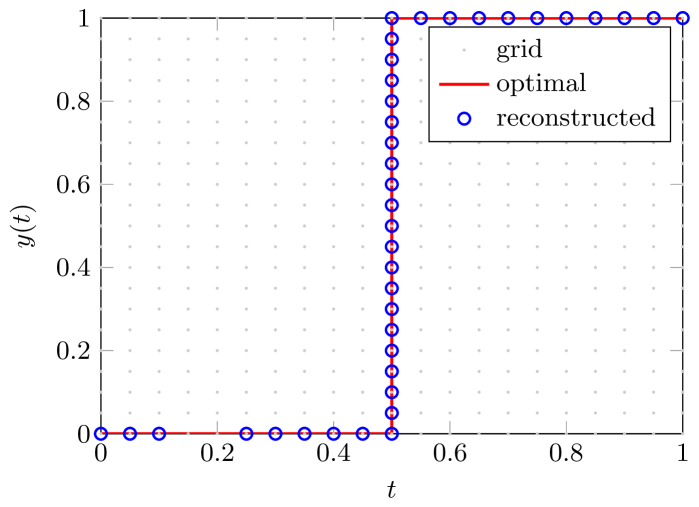
Figure 1: Reconstruction trajectory for Example 6.1.

6.2 Smeared impulses

We consider now optimal control problem (2), our second motivating example. This sequence tends weakly to the DiPerna-Majda measure given by

$$\sigma(dt)=2\,dt,\qquad\nu(du|t)=\frac{1}{2}\delta_{0}(du)+\frac{1}{2}\delta_{+\infty}(du),$$ (64)

with optimal trajectory given by $y(t)=t$.

In this case, one can avoid the use of lift variable $w_{0}$, since with the positivity constraint on $u$, we have simply $w_{0}=1-w_{1}$. Measure LP (42) is then expressed as

$$\inf_{\gamma,\mu_{1}} \langle\frac{(1-w)^{3}\,w^{2}}{(1-w)^{4}+w^{4}}+(1-w)\,(y_{1}-t)^{2},\gamma\rangle$$ (65)

s.t. $$\langle\frac{\partial v}{\partial t}(1-w)+\frac{\partial v}{\partial y}w,\gamma\rangle=\langle v(1,\cdot),\mu_{1}\rangle-v(0,y(0)),\>\>\forall v\in\mathbb{R}[t,y]$$

$$\gamma\in\mathcal{M}^{+}([0,1]^{3}),\>\>\mu_{1}\in\mathcal{M}^{+}(\mathbb{R})$$

Because we started with a cost rational in the control, there remains a rational expression in (65) despite the change of variables introduced in Section 4.1. This rational term can then treated by introducing the lifting variable $r=\frac{(1-w)^{3}\,w^{2}}{(1-w)^{4}+w^{4}}$, constrained algebraically via the equation $r((1-w)^{4}+w^{4})=(1-w)^{3}w^{2}$.

Solving the problem with GloptiPoly leads at the fourth relaxation leads to moments of the form

$$\left(\ell_{z}(t^{k})\right)_{k\in\mathbb{N}} =(2.0026,\,1.0026,\,0.6692,\,0.5026,\,0.4026,\,0.3359,\,\ldots),$$

$$\left(\ell_{z}(w^{k})\right)_{k\in\mathbb{N}} =(2.0026,\,1.0026,\,1.0012,\,0.9999,\,0.9985,\,0.9972,\,\ldots)$$

to be compared with the moments of the known optimal solution

$$\left(\langle t^{k},\gamma^{*}\rangle\right)_{k\in\mathbb{N}} =(2.0000,\,1.0000,\,0.6667,\,0.5000,\,0.4000,\,0.3333,\,\ldots),$$

$$\left(\langle w^{k},\gamma^{*}\rangle\right)_{k\in\mathbb{N}} =(2.0000,\,1.0000,\,1.0000,\,1.0000,\,1.0000,\,1.0000,\,\ldots).$$

The trajectory reconstructed with the method of Section 4.5 is given in Fig. 2. The reconstructed solution agrees with the true optimal solution.

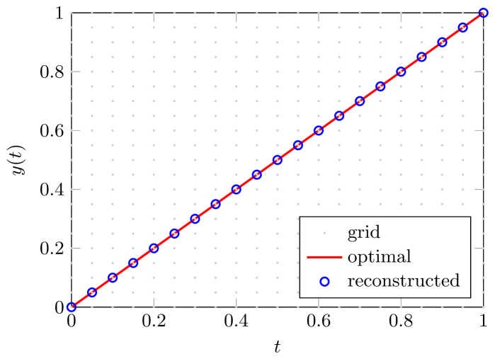
Figure 2: Reconstruction trajectory for Example 6.2.

6.3 Non-convex problem

We consider now a simplified planar orbital rendezvous problem constrained in a non-convex domain:

$$\inf_{u} \int_{0}^{1}\lvert u\rvert\,dt$$ (66)

s.t. $$\dot{y}_{1}=\pi\,y_{2},\>\>\dot{y}_{2}=-\pi\,y_{1}+u,$$

$$y(0)=(1/2,\>0),\>\>y(1)=(-1,\>0),$$

$$y_{1}^{2}(t)+y_{2}^{2}(t)\leq 2,\>\>y_{1}^{2}(t)+(y_{2}(t)-1/2)^{2}\geq 1/4,$$

$$u\in L^{1}([0,1]).$$

Instead of using $w_{0}:=1-\lvert w_{1}\rvert$ as for even $p$ in Section 4.1, one could instead use the lifting variable $r=\lvert w_{1}\rvert$, algebraically represented as $r^{2}=w_{1}^{2}$, $r\geq 0$. Then LP problem (42) is written as

$$\inf_{\gamma} \langle r,\gamma\rangle$$ (67)

s.t. $$\langle\frac{\partial v}{\partial t}(1-r)+\frac{\partial v}{\partial y_{1}}2\pi\,y_{2}(1-r)+\frac{\partial v}{\partial y_{2}}(-2\pi\,y_{1}(1-r)+w_{1}),\gamma\rangle$$

$$\quad\quad=v(1,y(1))-v(0,y(0)),\>\>\forall v\in\mathbb{R}[t,y]$$

$$\gamma\in\mathcal{M}^{+}(G)$$

with semi-algebraic set

$$\begin{array}[]{l}G=\{(t,y_{1},y_{2},w,r)\in\mathbb{R}^{5}:t(1-t)\geq 0,\>2-y^{2}_{1}-y^{2}_{2}\geq 0,\\ \quad\quad-1/4+y^{2}_{1}+(y^{2}_{2}-1/2)^{2}\geq 0,\>1-w^{2}_{1}\geq 0,\>r\geq 0,\>r^{2}=w^{2}_{1}\}\end{array}$$

defined accordingly to the constraints in the optimal control problem. The trajectory reconstructed from moments of the 6th relaxation is reported back on Fig. 3, with a relaxation cost of $p_{6}^{*}=0.824$. From this, it is easy to infer a candidate optimal trajectory involving an impulse of $\approx 0.273$ at $t=0$, followed by an impulse of $\approx-0.227$ at $t\approx 0.318$, followed by a control in feedback form of $u=y_{1}/(2y_{2}+1)$ to steer around the obstacle, followed by a free coasting arc. This admissible policy has a cost of $\approx 0.846$, which, given the relaxation cost, strongly suggests its global optimality.

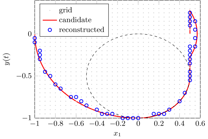
Figure 3: Reconstruction trajectory for the example of Ex. 6.3.

6.4 Weierstrass’ example

Consider the optimal control problem

$$\inf_{u} \int_{-1}^{1}t^{2}u^{2}\,dt$$ (68)

s.t. $$\dot{y}=u$$

$$y(-1)=-1,\quad y(1)=1$$

$$u\in L^{2}([-1,1]),\quad u(t)\geq 0.$$

Note the lack of coercivity in the cost integrand for $t=0$, so that the standing Assumptions 1 are not met. Following [33, Section 5.4] a minimizing sequence for this problem is

$$u^{k}(t)=\begin{cases}k&\mbox{if }\frac{-1}{k}\leq t\leq\frac{1}{k},\\ 0&\mbox{otherwise}.\end{cases}$$ (69)

Note however that $\lim_{k\rightarrow\infty}\int_{-1}^{1}\!(u^{k}(t))^{2}\,dt\rightarrow\infty$, such that the infimum cannot be attained by a DiPerna-Majda measure.

Solving the LP problem (42) with GloptiPoly leads to numerical issues, as the mass of $\gamma$ grows without bounds at each relaxation, as expected. We are currently investigating suitable analytical and numerical frameworks to cope with this problem. However, if one introduces an additional $L^{2}$ norm on the control, the problem becomes tractable by our approach. The new optimal minimizing sequence will obviously be different from (69).

References

• [1] L. Ambrosio, N. Fusco, D. Pallara. Functions of bounded variation and free discontinuity problems. Oxford University Press, UK, 2000.
• [2] E. J. Anderson, P. Nash. Linear programming in infinite-dimensional spaces: theory and applications. Wiley, 1987.
• [3] A. Barvinok. A course in convexity. American Mathematical Society, Providence, NJ, 2002.
• [4] A. Ben-Tal, A. Nemirovski. Lectures on modern convex optimization: analysis, algorithms, and engineering applications. SIAM, Philadelphia, 2001.
• [5] A. Blaquière. Impulsive optimal control with finite or infinite time horizon. Journal of Optimization Theory and Applications, 46:431–439, 1985.
• [6] A. Bressan, F. Rampazzo. On differential systems with vector-valued impulsive controls. Unione Matematica Italiana. Bollettino. B., 2(3):641–656, 1988.
• [7] A. E. Bryson, Y.C. Ho. Applied optimal control theory. Ginn & Co., Waltham, 1969.
• [8] M. Claeys. Mesures d’occupation et relaxations semi-définies pour la commande optimale. PhD thesis (in French), University of Toulouse, 2013.
• [9] M. Claeys, R. J. Sepulchre. Reconstructing trajectories from the moments of occupation measures. Proceedings of the IEEE Conference on Decision and Control, 2014.
• [10] M. Claeys, D. Arzelier, D. Henrion, J.-B. Lasserre. Measures and LMIs for non-linear optimal impulsive control. IEEE Transactions on Automatic Control, 59(5):1374-1379, 2014.
• [11] R. J. DiPerna, A. J. Majda. Oscillations and concentrations in weak solutions of the incompressible fluid equations. Communications in Mathematical Physics, 108(4):667-689, 1987.
• [12] V. A. Dykhta, O. N. Samsonyuk. Hamilton-Jacobi inequalities in control problems for impulsive dynamical systems. Proceedings of the Steklov Institute of Mathematics, 271(1):86–102, 2010.
• [13] H. O. Fattorini. Infinite dimensional optimization and control theory. Cambridge University Press, UK, 1999.
• [14] V. Gaitsgory, M. Quincampoix. Linear programming approach to deterministic infinite horizon optimal control problems with discounting. SIAM Journal On Control and Optimization, 48(4):2480-2512, 2009.
• [15] R. V. Gamkrelidze. Principles of optimal control theory. Plenum Press, New York, 1978.
• [16] W. M. Getz, D.H. Martin. Optimal control systems with state variable jump discontinuities. Journal of Optimization Theory and Applications, 31:195–205, 1980.
• [17] D. Henrion, M. Korda. Convex computation of the region of attraction of polynomial control systems. IEEE Transactions on Automatic Control, 59(2):297–312, 2014.
• [18] D. Henrion, J.-B. Lasserre, J. Löfberg. Gloptipoly 3: Moments, optimization and semidefinite programming. Optimization Methods and Software, 24(4-5):761–779, 2009.
• [19] M. Kružík, T. Roubíček. On the measures of DiPerna and Majda. Mathematica Bohemica, 122:383–399, 1997.
• [20] M. Kružík, T. Roubíček. Optimization problems with concentration and oscillation effects: relaxation theory and numerical approximation. Numerical Functional Analysis and Optimization, 20(5-6):511–530, 1999.
• [21] J. B. Lasserre, C. Prieur, D. Henrion. Nonlinear optimal control: numerical approximation via moments and LMI relaxations. Proc. IEEE Conf. Decision and Control and Europ. Control Conf., Sevilla, Spain, 2005.
• [22] J.-B. Lasserre, D. Henrion, C. Prieur, E. Trélat. Nonlinear optimal control via occupation measures and LMI relaxations. SIAM Journal on Control and Optimization, 47(4):1643–1666, 2008.
• [23] J.-B. Lasserre. Positive polynomials and their applications. Imperial College Press, London, UK, 2010.
• [24] R. Meziat, D. Patino, P. Pedregal. An alternative approach for non-linear optimal control problems based on the method of moments. Computational Optimization and Applications, 38(1):147–171, 2007.
• [25] R. Meziat, T. Roubíček, D. Patino. Coarse-convex-compactification approach to numerical solution of nonconvex variational problems. Numerical Functional Analysis and Optimization, 31(4):460–488, 2010.
• [26] B. Miller, E. Ya. Rubinovich. Impulsive control in continuous and discrete-continuous systems. Springer, Berlin, 2003.
• [27] M. Motta, F. Rampazzo. Space-time trajectories of nonlinear systems driven by ordinary and impulsive controls. Differential and Integral Equations, 8(2):269–288, 1995.
• [28] L. W. Neustadt. Optimization, a moment problem and nonlinear programming. SIAM Journal of Control, 2(1):33–53, 1964.
• [29] T. Roubíček. Relaxation in optimization theory and variational calculus. W. de Gruyter, Berlin, 1997.
• [30] T. Roubíček, M. Kružík. Adaptive approximation algorithm for relaxed optimization problems In Proceedings of ”Fast Solutions of Discrete Optimization Problems” held in WIAS, Berlin, May 8–12, 2000, (Eds. V. Schulz, K.-H. Hoffmann and R.H.W. Hoppe), Birkhäser, Basel, 2001
• [31] H. L. Royden, P. Fitzpatrick. Real analysis. 4th edition. Prentice Hall, NJ, 2010.
• [32] J. Souček. Spaces of functions on domain $\Omega$, whose $k$-th derivatives are measures defined on $\bar{\Omega}$. Časopis Pro Pěstování Matematiky, 97:10–46, 1972.
• [33] E. M. Stein, R. Shakarchi. Princeton lectures on analysis III. Real analysis: measure theory, integration, and Hilbert spaces. Princeton University Press, Princeton, NJ, 2005.
• [34] J. F. Sturm. Using SeDuMi 1.02, a Matlab toolbox for optimization over symmetric cones. Optimization Methods and Software, 11–12:625–653, 1999.
• [35] R. Vinter. Convex duality and nonlinear optimal control. SIAM Journal on Control and Optimization, 31(2):518–538, 1993.
• [36] R. Vinter, R. Lewis. The equivalence of strong and weak formulations for certain problems in optimal control. SIAM Journal on Control and Optimization, 16(4):546–570, 1978.
• [37] L. C. Young. Lectures on the calculus of variations and optimal control theory. W. B. Saunders Co., Philadelphia, NJ, 1969.