How to analyze stochastic time series obeying a 2nd order differential equation

Abstract

The stochastic properties of a Langevin-type Markov process can be extracted from a given time series by a Markov analysis. Also processes that obey a stochastically forced second order differential equation can be analyzed this way by employing a particular embedding approach: To obtain a Markovian process in 2N dimensions from a non Markovian signal in N dimensions, the system is described in a phase space that is extended by the temporal derivative of the signal. For a discrete time series, however, this derivative can only be calculated by a differencing scheme, which introduces an error. If the effects of this error are not accounted for, this leads to systematic errors in the estimation of the drift- and diffusion functions of the process. In this paper we will analyze these errors and we will propose an approach that correctly accounts for them. This approach allows an accurate parameter estimation and, additionally, is able to cope with weak measurement noise, which may be superimposed to a given time series.

I Introduction

Many dynamical systems can be modelled as continuous-time Markov processes $\mathbf{Y}(t)$ that are driven by Gaussian white noise $\boldsymbol{\xi}(t)$ with $\left<\xi_{i}(t)\right>\!=\!0$ and $\left<\xi_{i}(t)\xi_{j}(t^{\prime})\right>\!=\!\delta_{ij}\delta(t\!-\!t^{\prime})$. The temporal evolution of such a process obeys a Langevin equation – a first order ordinary differential equation (ODE) that is stochastically forced

$$\dot{\mathbf{Y}} = \mathbf{a}(\mathbf{Y})+\mathbf{b}(\mathbf{Y})\,\boldsymbol{\xi}(t).$$ (1)

Here and in the following Itô’s definition of a stochastic integral is used platen99 . Furthermore, a stationary stochastic process is looked at, whereas in general $\mathbf{a}$ and $\mathbf{b}$ may depend on time.

The Kramers–Moyal coefficients of the Fokker–Planck equation corresponding to Eq. (1) are denoted by $\mathbf{D}^{(1)}$ and $\mathbf{D}^{(2)}$ and commonly referred to as drift- and diffusion function respectively risken89 . These functions uniquely define the stochastic process and are related to $\mathbf{a}$ and $\mathbf{b}$ by

$$\mathbf{D}^{(1)}(\mathbf{y}) = \mathbf{a}(\mathbf{y}),\qquad\mathbf{D}^{(2)}(\mathbf{y})\;=\;\mathbf{b}(\mathbf{y})\mathbf{b}^{t}(\mathbf{y}).$$ (2)

It is possible to estimate $\mathbf{D}^{(1)}$ and $\mathbf{D}^{(2)}$ from a given time series of $\mathbf{Y}$ by a Markov analysis. This technique, also denoted as direct estimation method, has been introduced in the late 1990s friedrich97 ; siegert98 ; friedrich00 ; gradisek00 . Since then it has been successfully applied to problems out of many different fields. Reviews on Markov analysis and its applications can be found e.g. in friedrich11 ; friedrich08 .

The method is based on the fact that the moments $\mathbf{M}^{(k)}$ of the conditional process increments of $\mathbf{Y}$ can be expressed in terms of the Kramers–Moyal coefficients

$$\mathbf{M}^{(k)}(\mathbf{y},\tau) := \left<\big{[}\mathbf{Y}(t\!+\!\tau)\!-\!\mathbf{Y}(t)\big{]}^{k}\right>\big{|}_{\mathbf{Y}(t)=\mathbf{y}}$$ (3)

$$= \tau\mathbf{D}^{(k)}(\mathbf{y})+O(\tau^{2}),\quad k\;=\;1,2.$$ (4)

Here and in the following the $k$-th power of a vector denotes a $k$-fold dyadic product. The time argument $t$ of $\mathbf{M}^{(k)}$ is suppressed here because a stationary process is assumed. This assumption also allows a moment estimation from a single time series – ensemble averages can be replaced by time averages then (tacitly assuming ergodicity). For a non-stationary process an ensemble of time series would be needed (alternatively a windowing strategy could be applied, assuming a slowly varying time dependence).

The moments $\mathbf{M}^{(k)}$ (Eq. (3)) can be expressed in terms of moments $\mathbf{m}^{(k)}$ of the two-point probability density function (PDF) of $\mathbf{Y}$ at times $t$ and $t\!+\!\tau$. These moments $\mathbf{m}^{(k)}$ are defined as

$$\mathbf{m}^{(k)}(\mathbf{y},\tau) := \int_{\mathbf{s}}(\mathbf{s}\!-\!\mathbf{y})^{k}p(\mathbf{y},t;\mathbf{s},t\!+\!\tau)\,\boldsymbol{d}s,$$ (5)

where again the time argument $t$ is suppressed because of the assumption of stationarity. Using the well known relations $p(a;b)\!=\!p(b)p(a|b)$ and $\int_{a}f(a)p(a|b)\!=\!\left<f(A)|b\right>$ leads to

$$\mathbf{m}^{(k)}(\mathbf{y},\tau) = p(\mathbf{y},t)\,\mathbf{M}^{(k)}(\mathbf{y},\tau).$$ (6)

For $k\!=\!0$, this yields $m^{(0)}(\mathbf{y})\!=\!p(\mathbf{y},t)$ (suppressing the unneeded argument $\tau$ and taking into account the scalar nature of $m^{(0)}$). Consequently one can write $\mathbf{M}^{(k)}\!=\!\mathbf{m}^{(k)}/m^{(0)}$ and one obtains

$$\frac{\mathbf{m}^{(k)}(\mathbf{y},\tau)}{m^{(0)}(\mathbf{y})} = \tau\mathbf{D}^{(k)}(\mathbf{y})\!+\!O(\tau^{2}),\quad k=1,2.$$ (7)

The moments $\mathbf{m}^{(k)}(\mathbf{y},\tau)$ can directly be estimated from a given time series. In practise, this is usually done by applying a binning approach. Estimating the moments for a number of time increments $\tau$ then allows to solve Eq. (7) for $\mathbf{D}^{(k)}(\mathbf{y})$ in a least square sense. Usually a low order polynomial in $\tau$ is used for a fit of the right hand side, as the higher order terms in above equation are known to be powers of $\tau$ sampling02a ; sampling08 . This strategy will be denoted as standard Markov analysis (SMA) in the following.

Next, a stochastic process $\mathbf{X}(t)$ is looked at that obeys the second order ODE

$$\ddot{\mathbf{X}} = \mathbf{f}(\mathbf{X},\dot{\mathbf{X}})+\mathbf{g}(\mathbf{X},\dot{\mathbf{X}})\,\boldsymbol{\xi}(t),\quad\mathbf{X}\in\mathbb{R}^{N}.$$ (8)

Here $\boldsymbol{\xi}(t)$ denotes Gaussian white noise again. As Eq. (8) is a second order ODE, such a process is not Markovian, i.e., the statistics of its increments do not only depend on the value of $\mathbf{X}$ but also on its derivative. In an extended phase space, however, consisting of the values of $\mathbf{X}$ and $\dot{\mathbf{X}}$, the dynamic becomes Markovian. With the definitions

$$\mathbf{Y}_{1}(t) := \mathbf{X}(t),\quad\mathbf{Y}_{2}(t)\;:=\;\dot{\mathbf{X}}(t),$$ (9)

Eq. (8) can be written as a system of first order equations that define a Langevin process $\mathbf{Y}^{t}(t)\!:=\![\mathbf{Y}_{1}^{t}(t),\mathbf{Y}_{2}^{t}(t)]$ in $2N$ dimensions

$$\dot{\mathbf{Y}} = \begin{bmatrix}\dot{\mathbf{Y}}_{1}\\ \dot{\mathbf{Y}}_{2}\end{bmatrix}\;=\;\left[\begin{array}[]{l}\mathbf{Y}_{2}\\ \mathbf{f}(\mathbf{Y})+\mathbf{g}(\mathbf{Y})\,\boldsymbol{\xi}(t)\end{array}\right].$$ (12)

The Kramers–Moyal coefficients of the corresponding Fokker–Planck equation are simpler than in the general $2N$-dimensional case, as they are given by

$$\mathbf{D}^{(1)}(\mathbf{y}) = \begin{bmatrix}\mathbf{y}_{2}\\ \mathbf{f}(\mathbf{y})\end{bmatrix},\quad\!\mathbf{D}^{(2)}(\mathbf{y})\;=\;\begin{bmatrix}\mathbf{0}&\mathbf{0}\\ \mathbf{0}&\mathbf{g}\mathbf{g}^{t}\!(\mathbf{y})\end{bmatrix}\!.$$ (13)

Of cause, these coefficients can be estimated from a given time series of $\mathbf{Y}(t)$ by the above mentioned SMA. But therefor the values of $\mathbf{X}$ and $\dot{\mathbf{X}}$ must be given (Eq. (9)). For real word data this will not always be the case. Frequently only a series of ’positions’ $\mathbf{Y}_{1}(t)\!\equiv\!\mathbf{X}(t)$ will be given for a second order process obeying Eq. (8), while the corresponding ’velocities’ $\mathbf{Y}_{2}(t)\!\equiv\!\dot{\mathbf{X}}(t)$ are missing. It may, e.g., be hard to accurately meassure the velocities in a given experimental setup. Or it may not have been realized in advance that $\mathbf{X}(t)$ needs to be modelled as second order process. Or it may simply have been assumed that a highly resolved series of position values will provide sufficiently accurate information on the velocities.

If $\dot{\mathbf{X}}$ is missing, these velocity values need to be estimated numerically. This seems to be no major problem as $\mathbf{X}(t)$ is a continuously differentiable function. Its derivative can be estimated by a discrete differencing scheme with arbitrary accuracy – provided the step-size of the scheme (here and in the following denoted by $\theta$) can be chosen small enough. So for a ’sufficiently’ fine sampled series of positions the estimation-errors of the velocities will become negligible. The standard approach for an analysis, therefore, goes like this: Choose some small step-size $\theta$ and estimate the series $\mathbf{Y}_{2}$ using the given series $\mathbf{Y}_{1}$. Then apply a SMA to the resulting series $\mathbf{Y}$. This strategy will be denoted as standard embedding approach (SEA) in the following.

Such an approach, however, has its flaws. For a Markov analysis, the moments of process-increments will be looked at (see Eq. (3)). For these quantities the effects of the estimation errors will show to be of importance unless the step-size $\theta$ (used for velocity estimation) can be chosen much smaller than the time increment $\tau$ (used for increment calculation). At the same time, however, $\tau$ needs to be small compared to the characteristic time scale $T$ of the process under investigation. Otherwise the higher order terms in Eq. (7) can no longer be approximated by a low order polynomial. The requirement $\theta\!\ll\!\tau\!\ll\!T$ will only rarely be fulfilled in practise as it requires data with a very high temporal resolution (compared to the characteristic time scale $T$).

Also another source of errors has to be considered for real data: Any measurement noise that afflicts the values of $\mathbf{Y}_{1}$ will lead to an additional error in the estimation of $\mathbf{Y}_{2}$. For a differencing scheme with step-size $\theta$, this error will be proportional to $\theta^{-1}$, as will be seen later (assuming uncorrelated measurement noise). So even if the measurement noise is very small, and thus negligible for $\mathbf{Y}_{1}$ itself, it may become important in the estimation of $\mathbf{Y}_{2}$ for small values of $\theta$.

Above considerations imply that for real data neither the values of $\mathbf{Y}_{1}(t)$ nor that of $\mathbf{Y}_{2}(t)$ are known accurately. The ’noisy’ values, which are at hand, will be denoted by $\mathbf{Y}^{*}(t)$ in the following.

The aim of this paper is, to provide of a modified embedding approach (MEA) that accounts for the errors due to differencing scheme and meassurement noise. As a by-product also a quantitative description of the errors of the SEA will be found. However, only weak measurement noise can be accounted for. This restriction is a consequence of the perturbative approach that will be used. The requirements on the noise will be given later, but, roughly speaking, the noise must be negligible for the position values and its effect on the velocity increments may at most be of the same order as the effects of the driving stochastic force $\boldsymbol{\xi}$.

This paper is organized as follows: In Sec. II the observable moments $\mathbf{m}^{*(k)}$ of the noisy time series will be expressed in terms of moments of the noisy values $\mathbf{Y}^{*}(t)$ and $\mathbf{Y}^{*}(t\!+\!\tau)$ conditioned on the true value $\mathbf{Y}(t)$. Subsequently, based on a Taylor–Itô expansion, these conditional noisy values will be expressed in terms of process parameters, measurement noise and stochastic integrals of $\boldsymbol{\xi}$ in Sec. III. The resulting expressions, together with an assumption on the magnitude of the measurement noise, will lead to an explicit description of $\mathbf{m}^{*(k)}$ in Sec. IV then. This description will serve two purposes. Firstly, the effects of the reconstruction errors of a SEA can be quantified (Sec. V). Secondly, a MEA can be specified that allows an accurate estimation of the Kramers–Moyal coefficients and the properties of the measurement noise (Sec. VI). Subsequently a numerical test case will be specified in Sec. VII, which will be used to compare the results of SEA and MEA with and without measurement noise (Secs. VIII and IX).

II Moments of the noisy values

For a series of noisy values $\mathbf{Y}^{*}$ only the noisy counterparts $\mathbf{m}^{*(k)}$ of the moments $\mathbf{m}^{(k)}$ can be estimated. In analogy to Eq. (5) they can be defined as

$$\mathbf{m}^{*(k)}(\mathbf{y}^{*}) := \int_{\mathbf{s}}(\mathbf{s}\!\!-\!\mathbf{y}^{*})^{k}p(\mathbf{Y}^{*}\!\!=\!\mathbf{y}^{*}\!;\mathbf{Y}_{\tau}^{*}\!\!=\!\mathbf{s})\,\boldsymbol{d}s.$$ (14)

Here and in the following, the time arguments $t$ and $\tau$ are omitted to allow for a more compact notation. Stochastic variables implicitely refer to time $t$ now, and the shortcut $\mathbf{Y}_{\tau}^{*}$ is used to denote $\mathbf{Y}^{*}(t\!+\!\tau)$.

Next the moments $\mathbf{m}^{*(k)}$ need to be related to the process parameters and the properties of the measurement noise. As outlined in Sec. I, the first step will be, to express the moments $\mathbf{m}^{*(k)}$ in terms of moments of the conditional noisy values $\mathbf{Y}^{*}|_{\mathbf{Y}\!=\mathbf{y}}$ and $\mathbf{Y}_{\tau}^{*}|_{\mathbf{Y}\!=\mathbf{y}}$. This can be done as follows: First, the PDF in Eq. (14) is rewritten as

$$\!\!\!\!\!\!\!p(\mathbf{Y}^{*}\!\!=\!\mathbf{y}^{*}\!;\mathbf{Y}_{\tau}^{*}\!\!=\!\mathbf{s})\;\equiv\;\int_{\mathbf{y}}\rho(\mathbf{y})$$ (15)

$$\qquad\qquad\times\,p(\mathbf{Y}^{*}\!\!=\!\mathbf{y}^{*}\!;\mathbf{Y}_{\tau}^{*}\!\!=\!\mathbf{s}\big{|}\mathbf{Y}\!=\!\mathbf{y})\,\boldsymbol{d}y,$$ (16)

where $\rho(\mathbf{y})\!:=\!p(\mathbf{Y}\!=\!\mathbf{y})$ denotes the PDF of $\mathbf{Y}$. Inserting Eq. (15) and interchanging the order of integration thus allows to write the moments $\mathbf{m}^{*(k)}$ in the form

$$\mathbf{m}^{*(k)}(\mathbf{y}^{*}) = \int_{\mathbf{y}}\rho(\mathbf{y})\,\mathbf{F}^{(k)}(\mathbf{y}^{*}\!,\mathbf{y})\,\boldsymbol{d}y$$ (17)

with

$$\!\!\!\!\!\!\!\mathbf{F}^{(k)}(\mathbf{y}^{*}\!,\mathbf{y})\;=\;\int_{\mathbf{s}}(\mathbf{s}\!-\!\mathbf{y}^{*})^{k}$$ (18)

$$\qquad\qquad\times\,p(\mathbf{Y}^{*}\!\!=\!\mathbf{y}^{*}\!;\mathbf{Y}_{\tau}^{*}\!\!=\!\mathbf{s}\big{|}\mathbf{Y}\!=\!\mathbf{y})\,\boldsymbol{d}s.$$ (19)

Expressing the integral in Eq. (17) by a moment expansion yields (using summation convention)

$$m^{*(k)}_{i_{1},\ldots,i_{k}}(\mathbf{y}^{*}) = \sum_{\nu=0}^{\infty}\frac{(-1)^{\nu}}{\nu!}\frac{\partial}{\partial y^{*}_{j_{1}}}\cdots\frac{\partial}{\partial y^{*}_{j_{\nu}}}$$ (21)

$$\times\,\left[\rho(\mathbf{y}^{*})M^{(k,\nu)}_{i_{1},\ldots,i_{k},j_{1},\ldots,j_{\nu}}\!(\mathbf{y}^{*})\right],$$

where the moments are defined as

$$\mathbf{M}^{(k,\nu)}(\mathbf{y}^{*}) := \int_{\mathbf{z}}\mathbf{F}^{(k)}(\mathbf{z},\mathbf{y}^{*})\otimes(\mathbf{z}\!-\!\mathbf{y}^{*})^{\nu}\,\boldsymbol{d}z.$$ (22)

Here $\otimes$ denotes a dyadic product. Inserting the definition of $\mathbf{F}^{(k)}$ first leads to

$$\!\!\!\!\!\!\!\mathbf{M}^{(k,\nu)}(\mathbf{y}^{*})\;=\;\int_{\mathbf{s},\mathbf{z}}(\mathbf{s}\!-\!\mathbf{z})^{k}\otimes(\mathbf{z}\!-\!\mathbf{y}^{*})^{\nu}$$ (23)

$$\qquad\quad\quad\times\,p(\mathbf{Y}^{*}\!\!=\!\mathbf{z};\mathbf{Y}_{\tau}^{*}\!\!=\!\mathbf{s}\big{|}\mathbf{Y}\!=\!\mathbf{y}^{*})\,\boldsymbol{d}s\,\boldsymbol{d}z.$$ (24)

Using the relation $\int_{a}f(a)p(a|b)\!=\!\left<f(A)|b\right>$ then gives

$$\mathbf{M}^{(k,\nu)}(\mathbf{y}^{*}) = \left<(\mathbf{Y}_{\tau}^{*}\!\!-\!\mathbf{Y}^{*})^{k}\!\!\otimes\!(\mathbf{Y}^{*}\!\!-\!\mathbf{Y})^{\nu}\right>\!\big{|}_{\mathbf{Y}\!=\mathbf{y}^{*}}.$$ (25)

The general form of the observable moments $\mathbf{m}^{*(k)}$ therefore reads (dropping the asterisk on the parameter $\mathbf{y}$)

$$\!\!\!\!\!\!\!m^{*(k)}_{i_{1},\ldots,i_{k}}(\mathbf{y})\;=\;\sum_{\nu=0}^{\infty}\frac{(-1)^{\nu}}{\nu!}\frac{\partial}{\partial y_{j_{1}}}\cdots\frac{\partial}{\partial y_{j_{\nu}}}$$ (26)

$$\quad\times\left\{\rho(\mathbf{y})\big{<}[\mathbf{A}^{k}\!(\mathbf{y})]_{i_{1},\ldots,i_{k}}[\mathbf{B}^{\nu}\!(\mathbf{y})]_{j_{1},\ldots,j_{\nu}}\big{>}\right\}$$ (27)

with

$$\mathbf{A}(\mathbf{y}) := \mathbf{Y}_{\tau}^{*}\big{|}_{\mathbf{Y}\!=\mathbf{y}}\!-\mathbf{Y}^{*}\big{|}_{\mathbf{Y}\!=\mathbf{y}}\;,$$ (28a)

$$\mathbf{B}(\mathbf{y}) := \mathbf{Y}^{*}\big{|}_{\mathbf{Y}\!=\mathbf{y}}\!-\mathbf{y}.$$ (28b)

This is a quite general result – no information on how $\mathbf{Y}^{*}(t)$ and $\mathbf{Y}(t)$ are related is used so far. This will be done in the next section, where the conditional values of $\mathbf{Y}^{*}$ and $\mathbf{Y}_{\tau}^{*}$ will be expressed explicitly.

III Conditional values of $\mathbf{Y}^{*}$

In this section we will specify the assumptions on the measurement noise together with the details of the differencing scheme. This will allow to express the conditional values of $\mathbf{Y}^{*}$ and $\mathbf{Y}_{\tau}^{*}$ in terms of measurement noise and conditional values of $\mathbf{Y}_{1}$. Based on a Taylor–Itô expansion, these conditional values $\mathbf{Y}_{1}$ can then be expressed in terms of the driving stochastic force and process parameters.

To avoid confusion, time arguments will be given explicitly again in the following. However, the shortcut $(\ldots)|_{\mathbf{y}}$ will be used to indicate conditioning on $\mathbf{Y}(t)\!=\!\mathbf{y}$.

The given values $\mathbf{Y}^{*}_{1}(t)$ are assumed to be spoilt by additive, Gaussian distributed and temporally uncorrelated measurement noise $\boldsymbol{\Gamma}(t)$ with an expectation value of zero and covariance matrix $\mathbf{V}$

$$\left<\boldsymbol{\Gamma}(t)\right> = \mathbf{0},$$ (29a)

$$\left<\boldsymbol{\Gamma}(t)\boldsymbol{\Gamma}^{t}(t^{\prime})\right> = \delta_{t,t^{\prime}}\mathbf{V},\;\;\delta_{t,t^{\prime}}:=\left\{\begin{array}[]{ll}1\,,&\;t\!=\!t^{\prime}\\ 0\,,&\;t\!\neq\!t^{\prime}\end{array}\right..$$ (29d)

The noise is also assumed to be independent of $\boldsymbol{\xi}$ and $\mathbf{Y}$ (implying $\boldsymbol{\Gamma}(t)\big{|}_{\mathbf{y}}\!\equiv\boldsymbol{\Gamma}(t)$). The conditional values $\mathbf{Y}^{*}_{1}\big{|}_{\mathbf{y}}$ are thus given by

$$\mathbf{Y}^{*}_{1}(t\!+\!\Delta)\big{|}_{\mathbf{y}} := \mathbf{Y}_{1}(t\!+\!\Delta)\big{|}_{\mathbf{y}}+\boldsymbol{\Gamma}(t\!+\!\Delta).$$ (30)

For the reconstruction of $\mathbf{Y}_{2}$ a first order forward differencing scheme with a step-size of $\theta$, applied to the observable values $\mathbf{Y}^{*}_{1}$, will be used in the following. The conditional values $\mathbf{Y}^{*}_{2}\big{|}_{\mathbf{y}}$ therefore are given by

$$\mathbf{Y}^{*}_{2}(t\!+\!\Delta,\theta)\big{|}_{\mathbf{y}} := \frac{1}{\theta}\left[\mathbf{Y}_{1}(t\!+\!\Delta\!+\!\theta)\big{|}_{\mathbf{y}}\!-\mathbf{Y}_{1}(t\!+\!\Delta)\big{|}_{\mathbf{y}}\right]$$ (32)

$$+\frac{1}{\theta}\left[\boldsymbol{\Gamma}(t\!+\!\Delta\!+\!\theta)\!-\boldsymbol{\Gamma}(t\!+\!\Delta)\right].$$

The values $\mathbf{Y}_{1}\big{|}_{\mathbf{y}}$ at time $t\!+\!\Delta$ can be expressed by a Taylor–Itô expansion (see App. A)

$$\mathbf{Y}_{1}(t\!+\!\Delta)\big{|}_{\mathbf{y}} = \mathbf{y}_{1}+\mathbf{y}_{2}\,\Delta+\mathbf{f}(\mathbf{y})\frac{\Delta^{2}}{2}$$ (34)

$$+\mathbf{g}(\mathbf{y})\mathbf{I}^{t,\Delta}+\mathbf{R}^{t,\Delta}\!(\mathbf{y}).$$

Here $\mathbf{I}^{t,\Delta}$ denotes a vector of stochastic integrals that only depend on the realization of $\boldsymbol{\xi}$ in the interval $[t,t\!+\!\Delta)$. The components of this vector are of magnitude $O(\Delta^{3/2})$ and have an expectation value of zero. All other expansion terms are summarized in the remainder $\mathbf{R}^{t,\Delta}\!(\mathbf{y})$ with a magnitude of $O(\Delta^{2})$ and an expectation value of $O(\Delta^{3})$.

In summary, above results lead to the following expressions for $\mathbf{Y}^{*}\big{|}_{\mathbf{y}}$

$$\mathbf{Y}^{*}_{1}(t)\big{|}_{\mathbf{y}} = \mathbf{y}_{1}+\boldsymbol{\Gamma}(t),$$ (35a)

$$\mathbf{Y}^{*}_{1}(t\!+\!\tau)\big{|}_{\mathbf{y}} = \mathbf{y}_{1}+\mathbf{y}_{2}\,\tau+\mathbf{f}(\mathbf{y})\frac{\tau^{2}}{2}+\mathbf{g}(\mathbf{y})\mathbf{I}^{t,\tau}$$ (35c)

$$+\boldsymbol{\Gamma}(t\!+\!\tau)+\mathbf{R}^{t,\tau}\!(\mathbf{y}),$$

$$\mathbf{Y}^{*}_{2}(t,\theta)\big{|}_{\mathbf{y}} = \mathbf{y}_{2}+\mathbf{f}(\mathbf{y})\frac{\theta}{2}+\mathbf{g}(\mathbf{y})\frac{\mathbf{I}^{t,\theta}}{\theta}$$ (35e)

$$+\frac{\boldsymbol{\Gamma}(t\!+\!\theta)\!-\!\boldsymbol{\Gamma}(t)}{\theta}+\frac{\mathbf{R}^{t,\theta}\!(\mathbf{y})}{\theta},$$

$$\mathbf{Y}^{*}_{2}(t\!+\!\tau,\theta)\big{|}_{\mathbf{y}} = \mathbf{y}_{2}+\mathbf{f}(\mathbf{y})(\tau\!+\!\frac{\theta}{2})+\mathbf{g}(\mathbf{y})\frac{\mathbf{I}^{t,\tau\!+\!\theta}\!-\!\mathbf{I}^{t,\tau}}{\theta}$$ (35h)

$$+\frac{\boldsymbol{\Gamma}(t\!+\!\tau\!+\!\theta)\!-\!\boldsymbol{\Gamma}(t\!+\!\tau)}{\theta}$$

$$+\frac{\mathbf{R}^{t,\tau\!+\!\theta}\!(\mathbf{y})\!-\!\mathbf{R}^{t,\tau}\!(\mathbf{y})}{\theta}.$$

IV Moments $\mathbf{M}^{(k,\nu)}$

Now the moments $\mathbf{M}^{(k,\nu)}$ can be attacked. For a calculation of $\mathbf{M}^{(k,\nu)}$ explicit expressions for the vectors $\mathbf{A}$ and $\mathbf{B}$, as defined in Eq. (28), are needed. Using the results from the previous section (Eq. (35)) one finds

$$\mathbf{A}(\mathbf{y},\tau,\theta) = \begin{bmatrix}\mathbf{y}_{2}\,\tau+\mathbf{g}(\mathbf{y})\mathbf{I}^{t,\tau}+\boldsymbol{\Gamma}(t\!+\!\tau)-\boldsymbol{\Gamma}(t)+\mathbf{f}(\mathbf{y})\frac{\tau^{2}}{2}+\mathbf{R}^{t,\tau}\!(\mathbf{y})\\[3.00003pt] \mathbf{f}(\mathbf{y})\tau+\mathbf{g}(\mathbf{y})\frac{\mathbf{I}^{t,\tau\!+\!\theta}-\mathbf{I}^{t,\tau}-\mathbf{I}^{t,\theta}}{\theta}+\frac{\boldsymbol{\Gamma}(t\!+\!\tau\!+\!\theta)-\boldsymbol{\Gamma}(t\!+\!\tau)-\boldsymbol{\Gamma}(t\!+\!\theta)+\boldsymbol{\Gamma}(t)}{\theta}+\frac{\mathbf{R}^{t,\tau\!+\!\theta}\!(\mathbf{y})-\mathbf{R}^{t,\tau}\!(\mathbf{y})-\mathbf{R}^{t,\theta}\!(\mathbf{y})}{\theta}\end{bmatrix},$$ (36a)

$$\mathbf{B}(\mathbf{y},\tau,\theta) = \begin{bmatrix}\boldsymbol{\Gamma}(t)\\[3.00003pt] \mathbf{f}(\mathbf{y})\frac{\theta}{2}+\mathbf{g}(\mathbf{y})\frac{\mathbf{I}^{t,\theta}}{\theta}+\frac{\boldsymbol{\Gamma}(t\!+\!\theta)-\boldsymbol{\Gamma}(t)}{\theta}+\frac{\mathbf{R}^{t,\theta}\!(\mathbf{y})}{\theta}\end{bmatrix}.$$ (36b)

These expressions contain infinitely many terms, summarized in the remainders $\mathbf{R}$. To allow for a series truncation, a small parameter $\varepsilon$ is introduced in the following to express the magnitude of terms (it is tacitly assumed here that the problem is described in dimensionless form with $\mathbf{f}$ an $\mathbf{g}$ being of order $O(1)$). It will be assumed that $\tau$ and $\theta$ are of the same order of magnitude as $\varepsilon$ and that the measurement noise $\Gamma_{i}$ is of the same order as $\varepsilon^{3/2}$

$$\tau\overset{!}{=}O(\varepsilon),\quad\theta\overset{!}{=}O(\varepsilon),\quad V_{ij}\overset{!}{=}O(\varepsilon^{3}).$$ (37)

In a strict sense, the use of the Landau symbols here is not appropriate, because there is no functional relation between $\varepsilon$ and, e.g., $\tau$. Above notation is rather used to express the assumptions that, firstly, $\tau$, $\varepsilon$ and $\Gamma_{i}$ are small quantities, which allows to sort powers by magnitude (like e.g. $\tau^{2}\!\ll\!\tau$). Secondly, it is assumed that $\tau$, $\theta$ and $|\Gamma_{i}|^{2/3}$ are of ’compareable size’, where compareable size means that, when resticting to small exponents, also powers of different quantities can be sorted by size (like e.g. $\tau^{3}\!\ll\!\theta^{2}$ or $|V_{ij}|\!\ll\!\tau^{2}$). This will be sufficient for appropriate low order approximations.

With this assumptions the lowest order terms in $\mathbf{A}$ and $\mathbf{B}$ are of order $O(\varepsilon^{1/2})$. The magnitude of a moment $\mathbf{M}^{(k,\nu)}$, therefore, is given by (omitting arguments)

$$\mathbf{M}^{(k,\nu)} = \left<\mathbf{A}^{k}\otimes\mathbf{B}^{\nu}\right>\;=\;O(\varepsilon^{(k\!+\!\nu)/2}).$$ (38)

For a first order description of the moments $\mathbf{m}^{*(k)}$ thus only moments $\mathbf{M}^{(k,\nu)}$ with $k\!+\!\nu\leq 2$ need to be taken into account. Using Eq. (75) and the properties of $\boldsymbol{\Gamma}$, one finds

$$\mathbf{M}^{(0,0)} = 1,$$ (39a)

$$\mathbf{M}^{(0,1)} = \begin{bmatrix}\mathbf{0}\\ \frac{1}{2}\theta\mathbf{f}\end{bmatrix}\!+\!O(\varepsilon^{2}),$$ (39b)

$$\mathbf{M}^{(0,2)} = \begin{bmatrix}\mathbf{0}&\mathbf{0}\\ \mathbf{0}&\frac{1}{3}\theta\mathbf{g}\mathbf{g}^{t}\!+\!2\frac{\mathbf{V}}{\theta^{2}}\end{bmatrix}\!+\!O(\varepsilon^{2}),$$ (39c)

$$\mathbf{M}^{(1,0)} = \begin{bmatrix}\tau\mathbf{y}_{2}\\ \tau\mathbf{f}\end{bmatrix}\!+\!O(\varepsilon^{2}),$$ (40a)

$$\mathbf{M}^{(1,1)} = \begin{bmatrix}\mathbf{0}&\mathbf{0}\\ \mathbf{0}&\frac{\tau\!-\!\psi}{2}\mathbf{g}\mathbf{g}^{t}\!-\!(2\!+\!\delta_{\tau,\theta})\frac{\mathbf{V}}{\theta^{2}}\end{bmatrix}\!+\!O(\varepsilon^{2}),$$ (40b)

$$\mathbf{M}^{(2,0)} = \begin{bmatrix}\mathbf{0}&\mathbf{0}\\ \mathbf{0}&\psi\,\mathbf{g}\mathbf{g}^{t}\!+\!2(2\!+\!\delta_{\tau,\theta})\frac{\mathbf{V}}{\theta^{2}}\end{bmatrix}\!+\!O(\varepsilon^{2}),$$ (41)

with

$$\psi := \left\{\begin{array}[]{lcl}\tau^{2}/\theta-\frac{1}{3}\tau^{3}/\theta^{2}&,&\tau<\theta\\[3.00003pt] \tau-\frac{1}{3}\theta&,&\tau\geq\theta\end{array}\right..$$ (44)

Inserting these expressions into Eq. (21), finally, yields a first order description of the moments $\mathbf{m}^{*(k)}$ in terms of $\rho$, $\mathbf{f}$, $\mathbf{g}$ and $\mathbf{V}$. It turns out that derivatives with respect to components of $\mathbf{y}_{1}$ do not appear in the terms up to order $O(\varepsilon)$ – so for a first order description only the derivatives with respect to the components of $\mathbf{y}_{2}$ need to be considered. It also turns out that only the upper half of the vector $\mathbf{m}^{*(1)}$ and the upper quarter of the matrix $\mathbf{m}^{*(2)}$ need to be looked at (those components that correspond to moments of the increments of $\mathbf{Y}^{*}_{2}$). To take (syntactical) advantage of this reduction in dimensionality the notations

$$\hat{\partial}_{i} := \frac{\partial}{\partial y_{N\!+\!i}},\qquad\hat{m}^{(0)}\;:=\;m^{*(0)},$$ (45a)

$$\hat{m}^{(1)}_{i} := m^{*(1)}_{N\!+\!i},\qquad\;\hat{m}^{(2)}_{ij}\;:=\;m^{*(2)}_{N\!+\!i,N\!+\!j},$$ (45b)

are introduced, where $i$ and $j$ are in the range $1,\ldots,N$. The relevant equations can now be written compactly as

$$\hat{m}^{(0)}(\mathbf{y},\theta) = \rho-\frac{\theta}{2}\,\hat{\partial}_{i}[\rho f_{i}]+\frac{\theta}{6}\,\hat{\partial}_{i}\hat{\partial}_{j}[\rho\,(\mathbf{g}\mathbf{g}^{t})_{ij}]$$ (46b)

$$+\frac{V_{ij}}{\theta^{2}}\,\hat{\partial}_{i}\hat{\partial}_{j}\rho+O(\varepsilon^{2}),$$

$$\hat{m}^{(1)}_{i}(\mathbf{y},\tau,\theta) = \tau\rho f_{i}-\frac{1}{2}(\tau\!-\!\psi)\,\hat{\partial}_{j}[\rho\,(\mathbf{g}\mathbf{g}^{t})_{ij}]$$ (46d)

$$+(2\!+\!\delta_{\tau,\theta})\frac{V_{ij}}{\theta^{2}}\,\hat{\partial}_{j}\rho+O(\varepsilon^{2}),$$

$$\hat{m}^{(2)}_{ij}(\mathbf{y},\tau,\theta) = \psi\rho\,(\mathbf{g}\mathbf{g}^{t})_{ij}$$ (46f)

$$+2(2\!+\!\delta_{\tau,\theta})\frac{V_{ij}}{\theta^{2}}\,\rho+O(\varepsilon^{2}).$$

These equations directly relate the unknown quantities $\rho$, $\mathbf{f}$, $\mathbf{g}\mathbf{g}^{t}$ and $\mathbf{V}$ and the observable quantities $\hat{\mathbf{m}}^{(k)}$. The function argument of $\rho$, $\mathbf{f}$ and $\mathbf{g}$ is given by $\mathbf{y}$. The function $\psi$ depends on $\tau$ and $\theta$ and has a piecewise definition only, Eq. (44).

V Systematic errors of the standard embedding approach (SEA)

Next the SEA will be analyzed, using the final result of the previous section (Eq. (46)). Only the case without measurement noise, i.e. $\mathbf{V}\equiv\mathbf{0}$, will be looked at. This will show the ’pure’ effects of the reconstruction errors caused by the numerical estimation of $\mathbf{Y}_{2}$.

For a time series, where $\mathbf{Y}_{2}$ has been reconstructed by a first order forward differencing scheme with stepsize $\theta$, the observable moments $\hat{\mathbf{m}}^{(k)}$ are described by Eq. (46). Ignoring this result and attempting a Markov analysis as outlined in Sec. I will put the focus on the terms $\hat{\mathbf{m}}^{(k)}(\mathbf{y},\tau,\theta)/(\tau\hat{m}^{(0)}(\mathbf{y},\theta))$. According to Eq. (7), these terms should be finite-increment estimates of $\mathbf{f}$ and $\mathbf{g}\mathbf{g}^{t}$ ($k\!=\!1$ resp. $k\!=\!2$). In fact, however, the terms evaluate to

$$\frac{\hat{m}^{(1)}_{i}(\mathbf{y},\tau,\theta)}{\tau\hat{m}^{(0)}(\mathbf{y},\theta)} = f_{i}-\frac{1\!-\!\psi(\tau,\theta)/\tau}{2\hat{m}^{(0)}}\,\hat{\partial}_{j}\left[\hat{m}^{(0)}\,(\mathbf{g}\mathbf{g}^{t})_{ij}\right]$$ (47b)

$$+O(\varepsilon)$$

$$\frac{\hat{m}^{(2)}_{ij}(\mathbf{y},\tau,\theta)}{\tau\hat{m}^{(0)}(\mathbf{y},\theta)} = \frac{\psi(\tau,\theta)}{\tau}(\mathbf{g}\mathbf{g}^{t})_{ij}+O(\varepsilon).$$ (47c)

Trying to extrapolate these estimates to $\tau\!=\!0$ then becomes problematic. Instead of being approximately constant, as expected from Eq. (7), the values will show non-linear behaviour caused by the function $\psi/\tau$. For fixed $\theta$ this function starts linear with a value of zero at $\tau/\theta\!=\!0$, passes through $2/3$ at $\tau/\theta\!=\!1$ and approaches a value of one for $\tau/\theta\!\to\!\infty$. Simply fitting a low order polynomial to all estimates up to some maximum increment $\tau_{\text{max}}$ will thus, in general, under-estimate $\mathbf{g}\mathbf{g}^{t}$ (because of $|\psi/\tau|<1$). An error of compareable size (although with arbitrary sign) will occure when estimating $\mathbf{f}$.

In principle, however, the estimates for large $\tau$, i.e. where $\psi/\tau\approx 1$, could be used for a fit. On the other hand also the influence of higher order terms becomes stronger for large increments. Unless a time series is sampled with a very small timestep, such an approach will also fail to provide accurate estimates for $f_{i}$ and $(\mathbf{g}\mathbf{g}^{t})_{ij}$.

VI Modified embedding approach (MEA)

Based on Eq. (46), we now will propose a modified approach that takes into account the effects of the differencing scheme as well as the effects of measurement noise. An important point in this approach will be to keep the ratio of $\tau$ and $\theta$ fix. This provides an easy way to avoid problems caused by the non-linear term $\psi(\tau,\theta)$. In the following $\theta\!\equiv\!\tau$ is chosen. Equation (46) then reads

$$\hat{m}^{(0)}(\mathbf{y},\tau) = \rho-\frac{\tau}{2}\,\hat{\partial}_{i}[\rho f_{i}]+\frac{\tau}{6}\,\hat{\partial}_{i}\hat{\partial}_{j}[\rho\,(\mathbf{g}\mathbf{g}^{t})_{ij}]$$ (48b)

$$+\frac{V_{ij}}{\tau^{2}}\,\hat{\partial}_{i}\hat{\partial}_{j}\rho+O(\varepsilon^{2}),$$

$$\hat{m}^{(1)}_{i}(\mathbf{y},\tau,\tau) = \tau\rho f_{i}-\frac{\tau}{6}\,\hat{\partial}_{j}[\rho\,(\mathbf{g}\mathbf{g}^{t})_{ij}]$$ (48d)

$$+3\frac{V_{ij}}{\tau^{2}}\,\hat{\partial}_{j}\rho+O(\varepsilon^{2}),$$

$$\hat{m}^{(2)}_{ij}(\mathbf{y},\tau,\tau) = \tau\frac{2}{3}\rho\,(\mathbf{g}\mathbf{g}^{t})_{ij}$$ (48f)

$$+6\frac{V_{ij}}{\tau^{2}}\,\rho+O(\varepsilon^{2}).$$

A fixed ratio of $\tau$ and $\theta$ also leads to a simpler form of the higher order terms (see App. B). Each term of order $O(\varepsilon^{n})$ on the right hand side of Eq. (48) has the form

$$Q^{(n)} = c(\mathbf{y})\,\tau^{a}(\varepsilon^{3}/\tau^{2})^{b}$$ (49)

with

$$0\leq a\leq n,\quad b=n-a,\quad c=O(1).$$ (50)

Here the symbol $Q^{(n)}$ is used to denote such a term and $\varepsilon^{3}$ accounts for the assumption on the magnitude of $\mathbf{V}$. The functional form of $Q^{(n)}$ (with respect to $\tau$) can thus be described by a function-base ${\cal B}^{(n)}$ that consists of $n\!+\!1$ functions $\tau^{a-2b}$. As noted in App. B, this implies ${\cal B}^{(n)}\!\subset{\cal B}^{(n\!+\!3)}$ and thus puts a limit on the accuracy that can be achieved in least square fits of $\hat{\mathbf{m}}^{(k)}$. E.g. it is not possible to distinguish a first order term $c\tau$ and a fourth order term $c^{\prime}\tau^{3}(\varepsilon^{3}/\tau^{2})$ by their functional form.

In the following Eq. (48b) will be used in the form $\hat{m}^{(0)}\!=\!\rho+O(\varepsilon)$, i.e. the explicit results for the first order terms will not be used. This avoids the need to numerically calculate the derivatives that appear within these terms. Next, Eqs. (48d) and (48f) are divided by $\rho$. Replacing $\rho$ by $\hat{m}^{(0)}$ in the resulting left hand sides will only result in additionally terms of order $O(\varepsilon^{2})$ and higher for the right hand sides. One finds (omitting function arguments again)

$$\frac{\hat{m}^{(1)}_{i}}{\hat{m}^{(0)}} = \tau\tilde{f}_{i}+\frac{3V_{ij}\hat{\partial}_{j}\rho}{\tau^{2}\rho}+O(\varepsilon^{2}),$$ (51a)

$$\frac{\hat{m}^{(2)}_{ij}}{\hat{m}^{(0)}} = \tau\frac{2}{3}\,(\mathbf{g}\mathbf{g}^{t})_{ij}+\frac{6V_{ij}}{\tau^{2}}+O(\varepsilon^{2}),$$ (51b)

with the shortcut

$$\tilde{f}_{i} := f_{i}-\frac{\hat{\partial}_{j}[\rho\,(\mathbf{g}\mathbf{g}^{t})_{ij}]}{6\rho}.$$ (52)

The term $3V_{ij}(\hat{\partial}_{j}\rho)/(\tau^{2}\rho)$ in Eq. (51a) will now be expressed as $\tau^{-2}c_{i}$, where $c_{i}$ is a unknown constant (of order $O(\varepsilon^{3})$). Finally, it will be assumed that $\mathbf{V}$ is known. This assumption is not mandatory – $\mathbf{V}$ could be estimated using Eq. (51b) – but this quantity can be estimated more easily in advance by, e.g., analyzing the auto-covariance of $\mathbf{Y}^{*}_{1}$. The final set of equations now reads

$$\hat{m}^{(0)} = \rho+O(\varepsilon),$$ (53a)

$$\frac{\hat{m}^{(1)}_{i}}{\hat{m}^{(0)}} = \tau\tilde{f}_{i}+\frac{1}{\tau^{2}}c_{i}+O(\varepsilon^{2}),$$ (53b)

$$\frac{\hat{m}^{(2)}_{ij}}{\hat{m}^{(0)}}-\frac{6V_{ij}}{\tau^{2}} = \tau\frac{2}{3}(\mathbf{g}\mathbf{g}^{t})_{ij}+O(\varepsilon^{2}).$$ (53c)

The terms on the left hand sides can be estimated for different values of $\tau$ from a given time series. Choosing appropriate sets of regression functions thus allows to estimate $\rho$, $\tilde{\mathbf{f}}$ and $\mathbf{g}\mathbf{g}^{t}$ by a linear regression analysis. Once these quantities have been estimated, Eq. (52) can be used to finally calculate $\mathbf{f}$ (the derivative that appears in Eq. (52) can, e.g., be calculated using a density-weighted local polynomial fit of $\rho\mathbf{g}\mathbf{g}^{t}$).

The functional form of the higher order terms can be shown to still obey Eq. (49). Therefore $\{1,\tau,\tau^{-2}\}$, $\{\tau,\tau^{-2}\}$ and $\{\tau\}$ are appropriate function sets for Eq. (53a), (53b) and (53c) if terms up to order $O(\varepsilon)$ shall be taken into account. To also take into account second order terms, the functions $\{\tau^{2}\!,\tau^{-1}\!,\tau^{-4}\}$ must be added to the sets. In principle, also third order terms can be accounted for in Eq. (53b) and (53c) by also adding the functions $\{\tau^{3}\!,1,\tau^{-3}\!,\tau^{-6}\}$. In practise, however, a large number of regression functions and also large negative exponents lead to numerical problems. As a compromise, the terms can partially be accounted for. In the numerical example given later, e.g., only $\tau^{3}$ is used as regression function for third order terms.

VII Numerical test case

To check the analytical results and to compare the different embedding approaches, a numerical example is investigated now. As test case a scalar process $X(t$) is chosen that obeys the second order ODE

$$\ddot{X} = f(X,\dot{X})+g(X,\dot{X})\xi(t),$$ (54)

where $f$ and $g$ are defined as

$$f(X,\dot{X}) := -X-3\dot{X},\quad g(X,\dot{X})\;:=\;1.$$ (55)

Again $\xi(t)$ denotes Gaussian white noise with $\left<\xi(t)\xi(t^{\prime})\right>\!=\!\delta(t\!-\!t^{\prime})$. Above ODE can be rewritten as a system of first order ODEs for a $2D$ process $\mathbf{Y}(t)$, the components of which are given by position $Y_{1}\!\equiv\!X$ and velocity $Y_{2}\!\equiv\!\dot{X}$ of the $1D$ process $X(t)$

$$\dot{Y}_{1} = Y_{2},$$ (56a)

$$\dot{Y}_{2} = -Y_{1}-3Y_{2}+\xi.$$ (56b)

These equations describe an Ornstein–Uhlenbeck process in two dimensions and can be solved analytically. The characteristic time scales of the auto-covariance of $\mathbf{Y}$ are found to be $(3\!+\!\sqrt{5})/2\!\approx\!2.618$ and $(3\!-\!\sqrt{5})/2\!\approx\!0.382$. The values of $\mathbf{Y}$ are Gaussian distributed and have a variance of $\left<\mathbf{Y}\mathbf{Y}^{t}\right>\!=\!\mathbf{Id}/6$.

For this process a time series of $\mathbf{Y}$, consisting of $10^{7}$ values, sampled with a time increment $\Delta t\!=\!0.01$, is generated. Excerpts of the resulting series for $Y_{1}$ and $Y_{2}$ are shown in Figs. (1) and (2). Here also a basic problem of the SEA can be seen, which was noted in Sec. (I) and quantified in Sec. (V): Even if a series is sampled sufficiently fine to allow an ’accurate’ estimation of $Y_{2}$ by a numerical differencing scheme, the velocity increments (for time increment $\tau$) will still show notable errors for small $\tau$. This error depends on the ratio $\theta/\tau$ (here $\theta\!=\!\Delta t$) and its effects can be quantified by the function $\psi$ in Eq. (47).

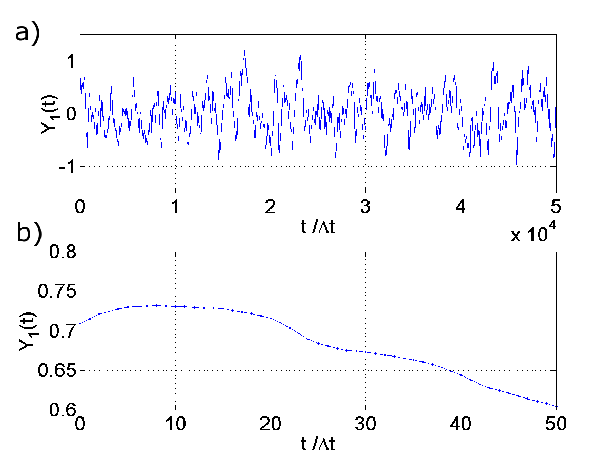
Figure 1: Excerpt of the generated series of position values $Y_{1}$ (a). A zoomed-in view (b) shows that the signal in fact is smooth and thus allows to numerically estimate its derivative if the sampling time step $\Delta t$ is sufficiently small.

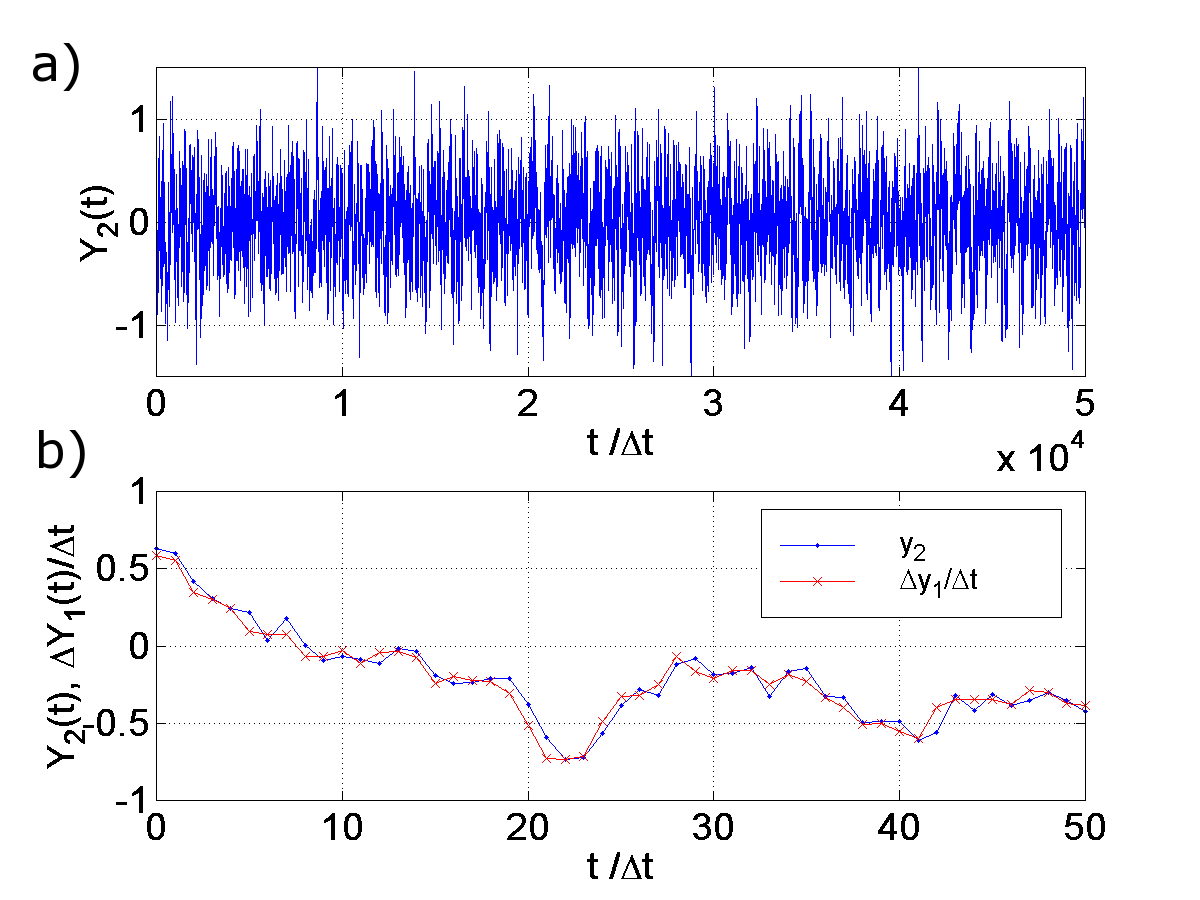
Figure 2: Excerpt of the generated series of velocity values $Y_{2}$ (a). In the zoomed-in view (b) additionally the numerically estimated derivative of $Y_{1}$ is shown. Allthough the values of both series (true and estimated) quite accurately match, there are notable differences for the small scale increments.

To obtain a baseline for the accuracy that can be achieved with the given data, a SMA is applied to the true $2D$ series $\mathbf{Y}$ first. Here and for subsequent analyses a binning approach is used, where the region $[-1,1]\times[-1,1]$ of the $(y_{1},y_{2})$-plane is covered by $30\times 30$ bins. For one of these bins the estimated moments of the conditional velocity increments are shown in Fig. (3).

Figure 3: First (a) and second moment (b) of the conditional velocity increments (obtained by a SMA). The estimated values (circles) are scaled by $\tau^{-1}$. The corresponding fits are shown as solid curves. Estimates are taken at $(y_{1},y_{2})\!=\!(-0.1,-0.2333)$. Here $f$ and $g^{2}$ have values of $0.8$ and $1.0$ respectively (dashed lines).

Actually the moments in Fig. (3) are scaled by $\tau^{-1}$, as is usually done for their visual presentation. This allows to interprete the estimation of $f$ and $g^{2}$ as ’extrapolating the scaled moments to $\tau\!=\!0$’. Later on, however, when measurement noise enters the scene, a more general interpretation will be needed, where $f$ and $g^{2}$ are found by a linear regression strategy. Of cause this interpretation is also valid in the given setup. The values of $f$ and $g^{2}$ are given by the coefficients of the linear part (in $\tau$) of the conditional moments $m^{(1)}_{2}/m^{(0)}$ and $m^{(2)}_{22}/m^{(0)}$ respectively (see Eq. (7)).

In the following the regression functions $\{\tau,\tau^{2}\}$ and $\{\tau,\tau^{2},\tau^{3}\}$ are used to fit the estimated first and second conditional moments (this corresponds to fitting a linear function to the values in Fig.(3a) and a quadratic function to those in Fig.(3b)). The maximum increment that is used for these fits is chosen as $\tau_{\text{max}}\!=\!15\Delta t$. The resulting estimates for $f$ and $g^{2}$ are shown in Fig. (4). In Fig. (5) the absolute errors $\delta f$ and $\delta g^{2}$ of these estimates are shown. In regions with low density (as noted above, the PDF of $\mathbf{Y}$ is a symmetric Gaussian with a standard deviation of $\approx 0.408$) fluctuations become larger but there is no obvious bias of the results.

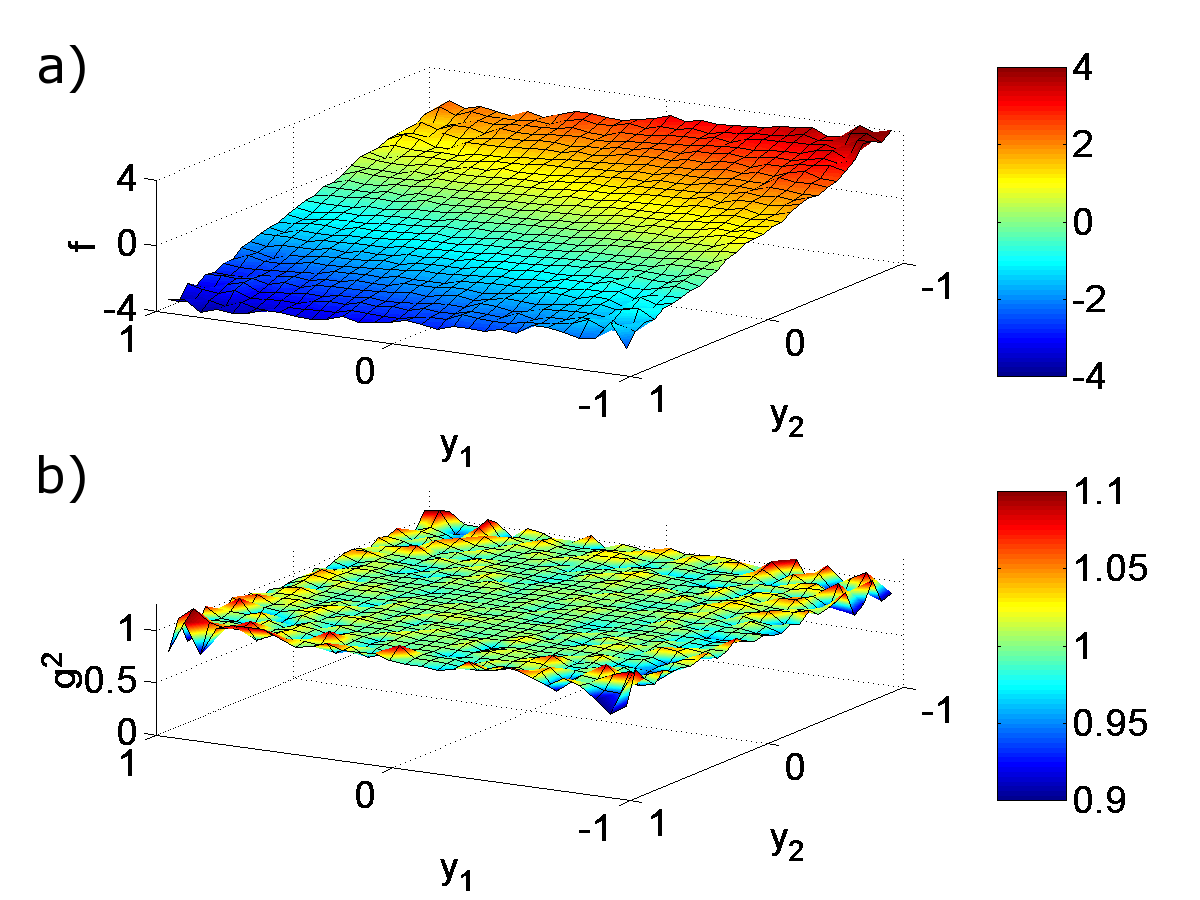
Figure 4: Estimates for $f$ and $g^{2}$ (a, b), obtained by a SMA.

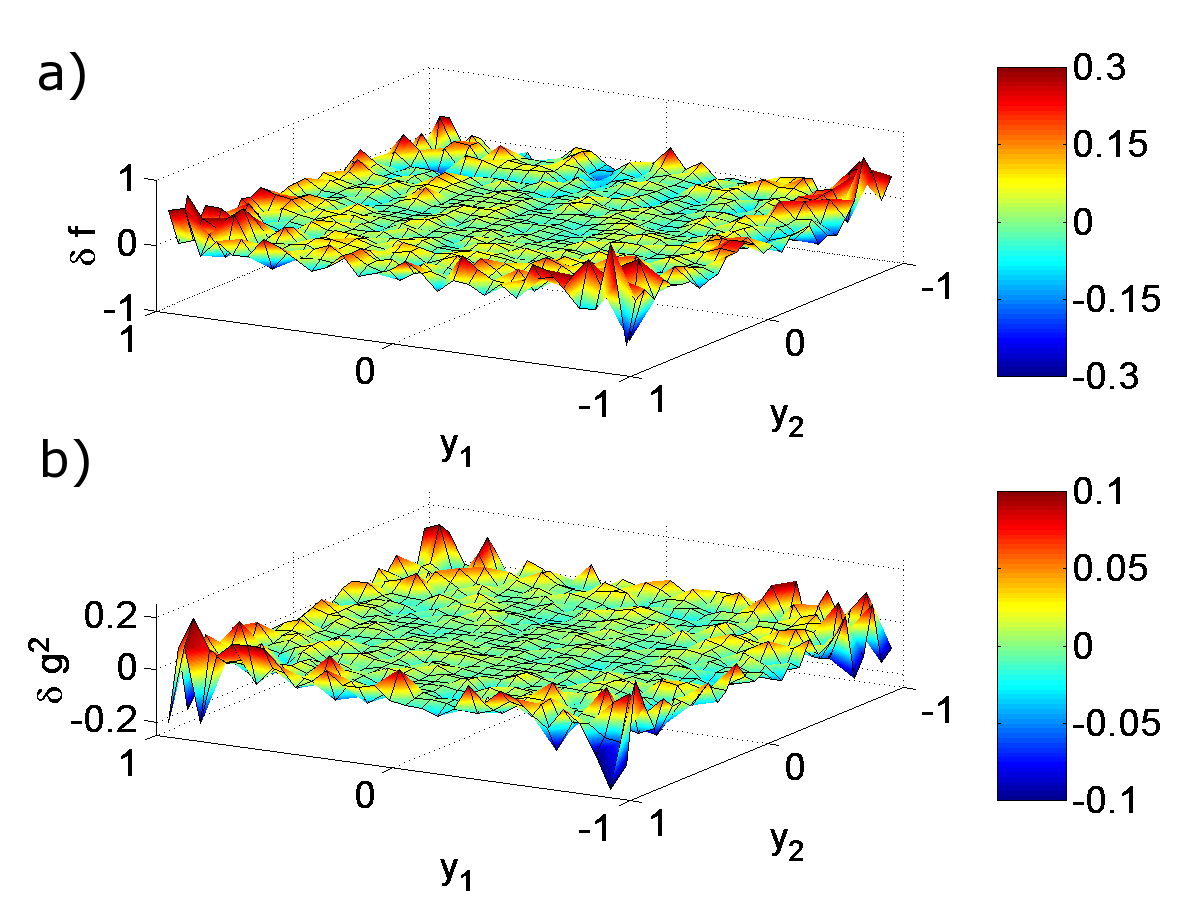
Figure 5: Absolute errors of the estimates for $f$ and $g^{2}$ (a, b), obtained by a SMA.

VIII Embedding approaches without measurement noise

Next the results of the different embedding approaches are looked at. First a SEA is used to perform an analysis solely based on the $1D$ series of positions $Y_{1}$. The corresponding velocity values $Y_{2}$ are estimated by a first order forward differencing scheme with a step size of $\theta\!=\!\Delta t$ and the resulting $2D$ series then is analyzed by a SMA.

As is shown in Fig. (6), the estimated moments of the conditional velocity increments behave quite different, compared to those obtained from the true $2D$ series (shown in Fig. (3)). As expected from Eq. (47), the moments show strongly nonlinear behaviour for small increments $\tau$. For an estimation of $f$ and $g^{2}$, therefore, only increments with $5\leq\tau/\Delta t\leq 15$ are used. Least square fits are performed using the same sets of regression functions as in the previous section. The absolute errors $\delta f$ and $\delta g^{2}$ of the resulting estimates are shown in Fig. (7). Of cause, the fluctuations become larger now as fewer increments are used for the fits. But, more importantly, it is obvious that $g^{2}$ is systematically under-estimated. And also the estimates for $f$ clearly show a significant bias that is approximately linear in $y_{2}$.

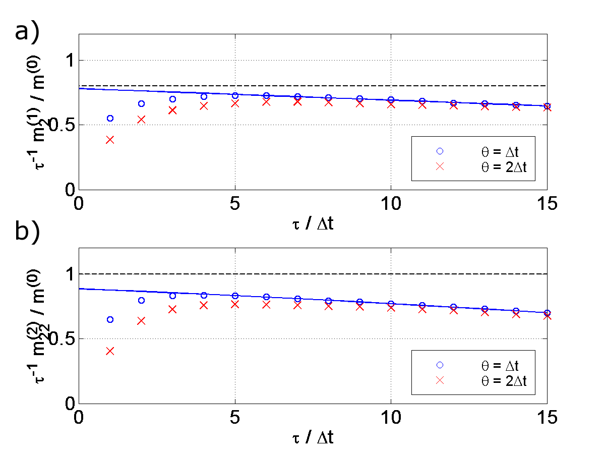
Figure 6: First (a) and second moment (b) of the conditional velocity increments (obtained by a SEA with $\theta\!=\!\Delta t$). The estimated values (circles) are scaled by $\tau^{-1}$. The corresponding fits are shown as solid curves. Additionally, the estimates obtained by a SEA with $\theta\!=\!2\Delta t$ are shown (crosses). Estimates are taken at $(y_{1},y_{2})\!=\!(-0.1,-0.2333)$. Here $f$ and $g^{2}$ have values of $0.8$ and $1.0$ respectively (dashed lines).

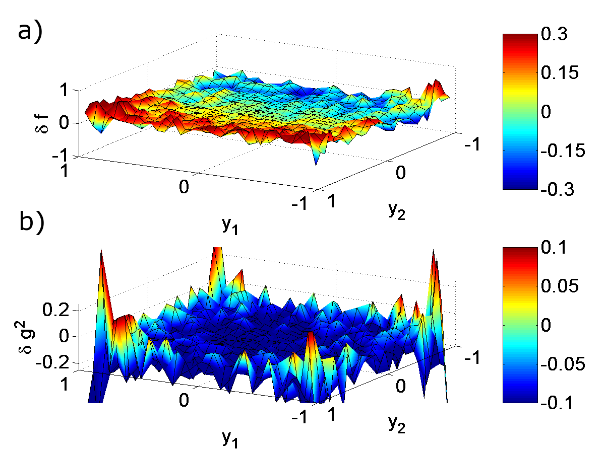
Figure 7: Absolute errors of the estimates for $f$ and $g^{2}$ (a, b), obtained by a SEA.

Using a SEA also affects the estimates for the process density $\rho$. It would be missleading, however to compare the estimates $m^{(0)}$ to the true density $\rho$, as is done in Fig. (8a). To a large extent the observed errors are caused by finite size effects and not by the reconstruction approach (the binned density of the true $2D$ series would show very similar errors). To assess the errors that are introduced by the embedding approach, the estimates $m^{(0)}$ thus should be compared to the binned density of the $2D$ series. This is done in Fig. (8b), where the erros are found to be biased by a hyperbolic function in $y_{1}$ and $y_{2}$.

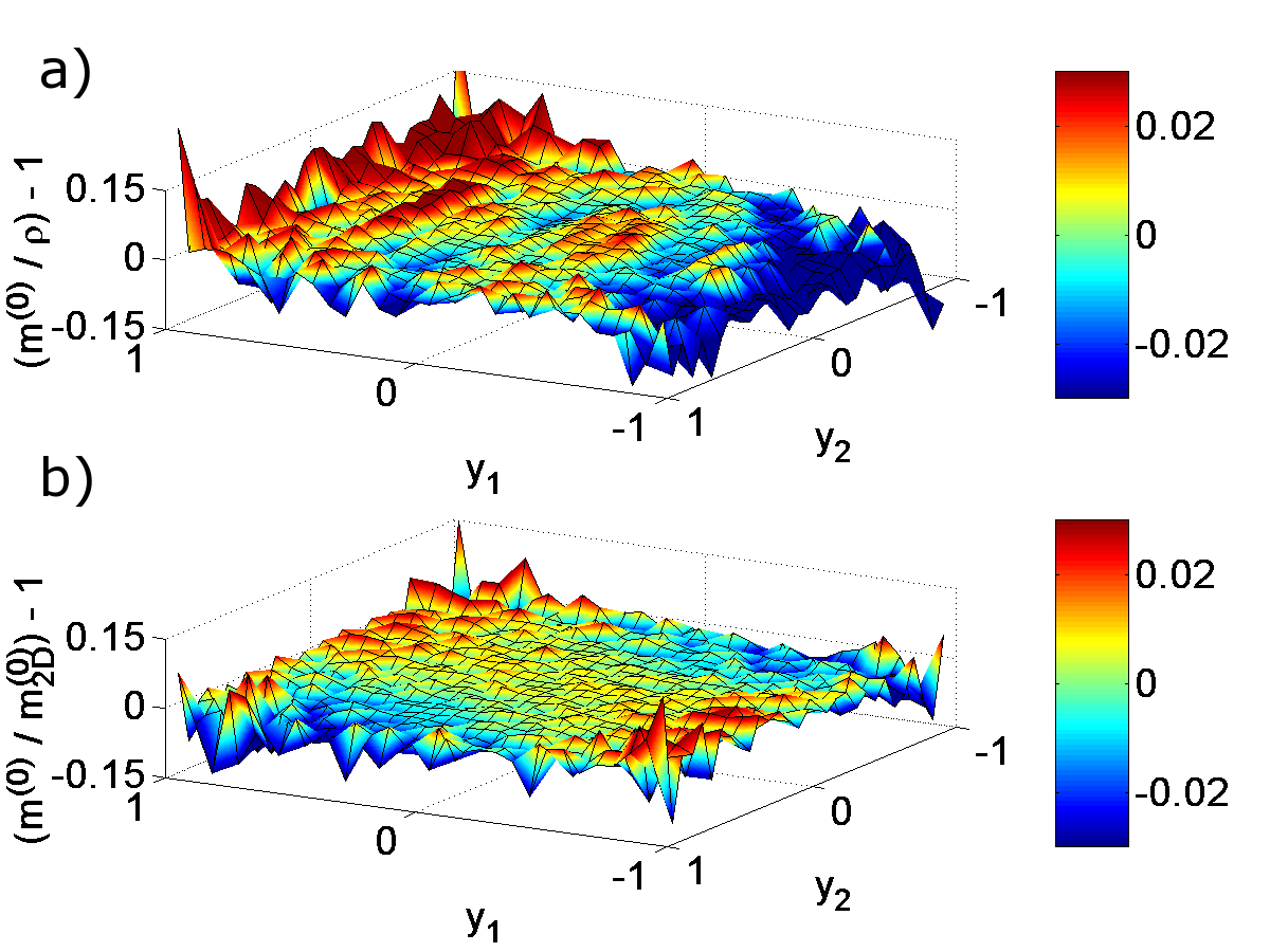
Figure 8: Relative errors of the estimated density values, obtained by a SEA. In (a) errors relative to the true density $\rho$ are shown. In (b) errors are relative to the binned density of the $2D$ series.

Now a MEA, as proposed in Sec. (VI), is applied. Again the analysis is purely based on the $1D$ series of positions $Y_{1}$. Opposed to a SEA, however, velocities are no longer estimated by a differencing scheme with a fixed step size. Instead, velocities and velocity increments for time increment $\tau$ are estimated using the step size $\theta\!=\!\tau$. Using a binning approach, it is not much more effort than for a SEA to implement the calculation of the density $m^{(0)}$ and of the conditional moments $m^{(1)}_{1}/m^{(0)}$ and $m^{(2)}_{22}/m^{(0)}$. In pseudo-code this reads:

for i=1:n-kmax  % n data-points
  for k=1:kmax  % kmax increments
    pos = x[i]  % x is data array
    velo = (x[i+k]-x[i])/k/dt  % sampling step dt
    dvelo = (x[i+2*k]-2*x[i+k]+x[i])/k/dt
    idx = getBinIndex(pos,velo)
    if(isValid(idx))
      m0[idx][k] += 1
      m1[idx][k] += dvelo
      m2[idx][k] += dvelo*dvelo
    end
  end
end
for idx=1:idxmax  % loop over all indicees
  for k=1:kmax
    m1[idx][k] /= m0[idx][k] % 1st cond. moment
    m2[idx][k] /= m0[idx][k] % 2nd cond. moment
    m0[idx][k] /= (n-kmax)*binSize % density
  end
end

Estimates for density and conditional moments obtained by a MEA are shown in Fig. (9). As expected from Eq. (51), the scaled moments now approach $\tilde{f}$ and $2g^{2}\!/3$ respectively for $\tau\!\to\!0$. Also the density $m^{(0)}$ now depends on $\tau$ and approaches the density of the $2D$ series.

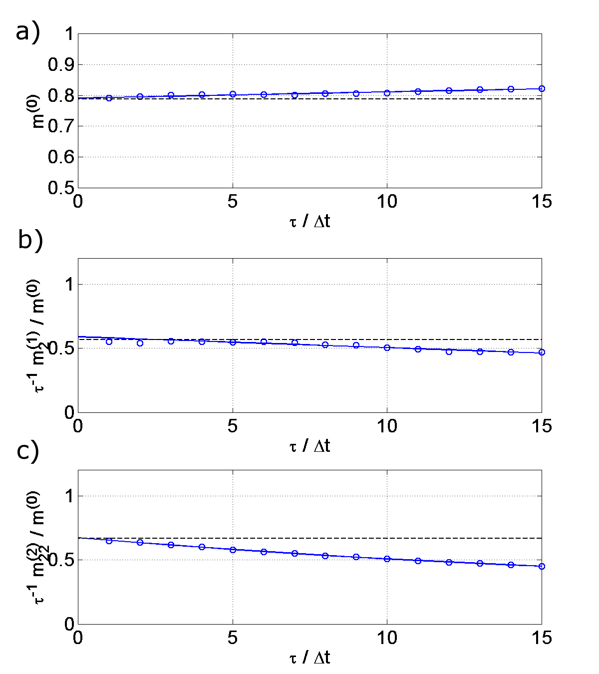
Figure 9: Estimated densities (a) and estimated moments (scaled by $\tau^{-1}$) of the conditional velocity increments (b, c). The estimates (circles) have been obtained by a MEA. The corresponding fits are shown as solid curves. Estimates are taken at $(y_{1},y_{2})\!=\!(-0.1,-0.2333)$. Here $\tilde{f}$ (see Eq. (52)) and $2g^{2}\!/3$ have values of $0.5667$ and $0.6667$ respectively and the binned density of the $2D$ series has a value of $0.7873$ (dashed lines).

All increments up to $\tau_{\text{max}}\!=\!15\Delta t$ are used for the least square fits. The regression functions $\{1,\tau\}$ are used to fit the density estimates. For the fits of the estimated first and second conditional moments again the functions $\{\tau,\tau^{2}\}$ respectively $\{\tau,\tau^{2},\tau^{3}\}$ are used. There is no need to add functions like $\tau^{-2}$, as still a case without measurement noise is looked at. The errors of the resulting estimates for $\rho$, $f$ and $g^{2}$ are shown in Fig. (10). Opposed to a SEA, shown in Fig. (7), no obvious biasing of the estimates can be observed and the fluctuations of $\delta f$ and $\delta g^{2}$ are compareable to those observed in an analysis of the $2D$ series using a SMA.

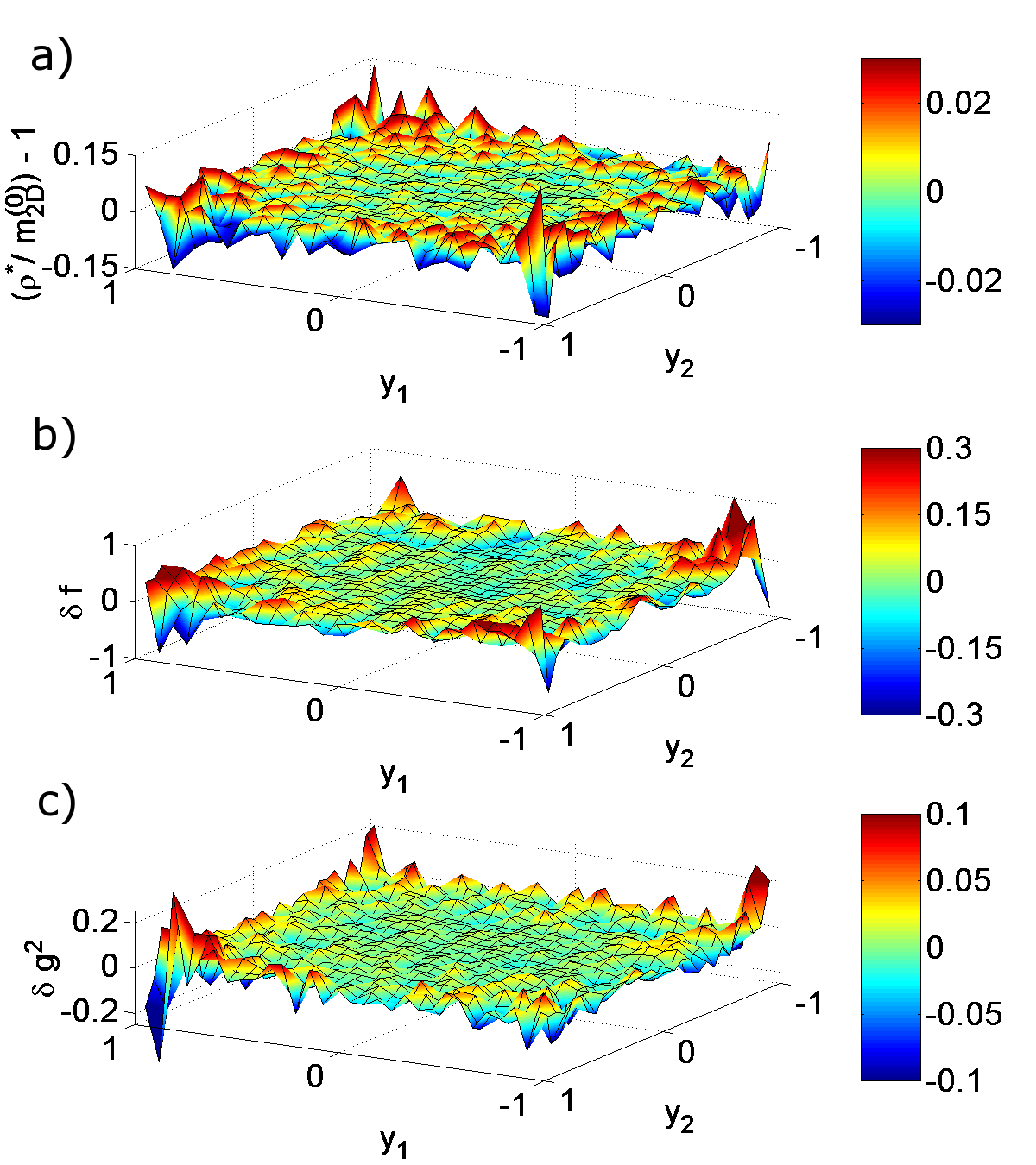
Figure 10: Relative error of the estimated density $\rho$ (a) and absolute errors of the estimates for $f$ and $g^{2}$ (b, c), obtained by a MEA. Errors in (a) are relative to the binned density of the $2D$ series.

IX Embedding approaches with measurement noise

So far, only data without measurement noise as been analyzed. Next, a series of ’noisy’ values $Y_{1}^{*}$ is generated by adding Gaussian, uncorrelated noise with a variance of $V\!=\!1.6667\times 10^{-7}$ (this corresponds to a noise-to-signal amplitude ratio of $10^{-3}$) to the series $Y_{1}$. This noisy series $Y_{1}^{*}$ is then analyzed – first by applying a SEA and next by applying a MEA.

Moments obtained by a SEA are shown in Fig. (11). Due to the measurement noise the scaled moments now diverge for $\tau\!\to\!0$. For an estimation of $f$ and $g^{2}$, therefore, again only increments with $5\leq\tau/\Delta t\leq 15$ are used. Least square fits again are performed using the functions $\{\tau,\tau^{2}\}$ and $\{\tau,\tau^{2},\tau^{3}\}$ respectively. The absolute errors $\delta f$ and $\delta g^{2}$ of the resulting estimates are shown in Fig. (12). It turns out that $g^{2}$ is systematically over-estimated now. The estimates for $f$ still show a significant bias that is approximately linear in $y_{2}$ – allthough the bias now has switched sign.

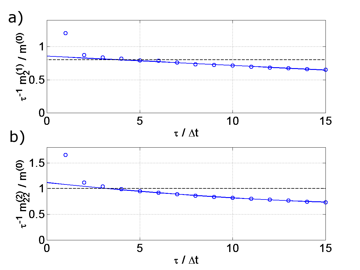
Figure 11: First (a) and second moment (b) of the conditional velocity increments of the noisy series $Y_{1}^{*}$ (obtained by a SEA with $\theta\!=\!\Delta t$). The estimated values (circles) are scaled by $\tau^{-1}$. The corresponding polynomial fits are shown as solid curves. Estimates are taken at $(y_{1},y_{2})\!=\!(-0.1,-0.2333)$. Here $f$ and $g^{2}$ have values of $0.8$ and $1.0$ respectively (dashed lines).

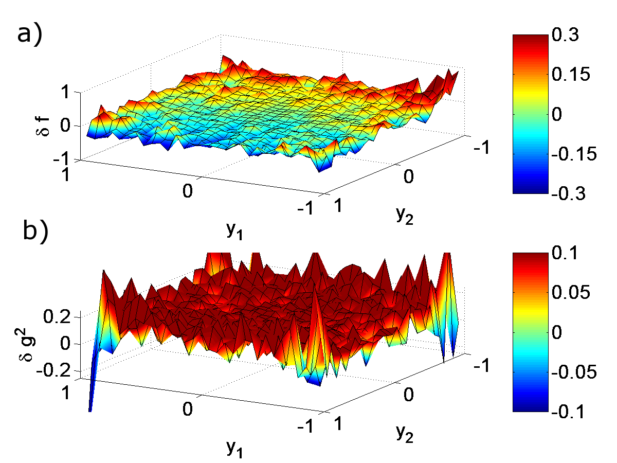
Figure 12: Absolute errors of the estimates for $f$ and $g^{2}$ (a,b), obtained by using a SEA for the noisy series $Y_{1}^{*}$.

Finally our proposed MEA is applied to the series $Y_{1}^{*}$, what leads to estimates for density and conditional moments as shown in Fig. (13). For $\tau\!\to\!0$ the moments are diverging because of the terms proportional to $\tau^{-2}$ (and other higher order terms proportional to negative powers of $\tau$), as described by Eq. (51). It is thus neccessary now, to add appropriate regression functions that account for these terms: For density estimation, all terms up to order $O(\varepsilon)$ are accounted for by using the functions $\{1,\tau,\tau^{-2}\}$. Fits of the first conditional moments (yielding an estimate for $\tilde{f}$) are performed using the regression functions $\{\tau,\tau^{-2},\tau^{2},\tau^{-1},\tau^{-4}\}$, i.e. considering terms up to order $O(\varepsilon^{2})$. Fits of the second conditional moments, finally, (yielding an estimate for $2g^{2}\!/3$) are performed using the regression functions $\{\tau,\tau^{2},\tau^{-1},\tau^{-4},\tau^{3}\}$. This choice needs some explanation. Firstly, only $\tau^{3}$ is present to account for third order terms. This is a compromise for numerical reasons – it reduces the number of regression functions and avoids numerical problems with large negative powers of $\tau$. Secondly, the first order term $6V/\tau^{2}$ is not accounted for by any regression function. This term is assumed to be known and thus does not need to be estimated. The value of $V$ is estimated in advance by extrapolating the auto-covariance function of $Y_{1}^{*}$ to $\tau\!=\!0$ and then taking the difference to $\left<Y_{1}^{*2}\right>$. Estimates for $V$ that are obtained this way are accurate within about five percent, as has been checked numerically.

Using above sets of regression functions and all increments up to $\tau_{\text{max}}\!=\!15\Delta t$ then leads to estimates for $f$ and $g^{2}$, the absolute errors of which are shown in Fig. (14). The estimates are quite heavily fluctuating now. But – at least to the bare eye – the results seem not to be biased.

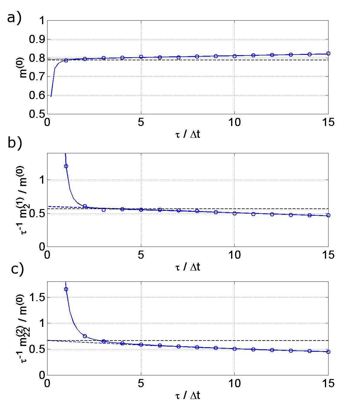
Figure 13: Estimated densities (a) and estimated moments (scaled by $\tau^{-1}$) of the conditional velocity increments (b, c) of the noisy series $Y_{1}^{*}$. The estimates (circles) have been obtained by a MEA. The corresponding fits are shown as solid curves. The non-diverging parts of these fits are shown as dashed curves. Estimates are taken at $(y_{1},y_{2})\!=\!(-0.1,-0.2333)$. Here $\tilde{f}$ (see Eq. (52)) and $2g^{2}\!/3$ have values of $0.5667$ and $0.6667$ respectively and the binned density of the $2D$ series has a value of $0.7873$ (dashed lines).

Figure 14: Absolute errors of the estimates for $f$ and $g^{2}$ (a, b), obtained by using a MEA for the noisy series $Y_{1}^{*}$.

X Summary of numerical results

Solid quantitative results for biases of the results of the different analyses that have been performed would require an averaging over a large number of analyses of independent realizations of $\mathbf{Y}$. Instead, a simpler approach is chosen to numerically compare the results. A polynomial $P$ with

$$P=a\!+\!b_{1}y_{1}\!+\!b_{2}y_{2}\!+\!c_{11}y_{1}^{2}\!+\!c_{12}y_{1}y_{2}\!+\!c_{22}y_{2}^{2}$$ (57)

is fitted to the results for $f$ and $g^{2}$ using a density weighted least square fit. According to Eq. (55) the only non-zero coefficients for $f$ should be $b_{1}\!=\!-1$ and $b_{2}\!=\!-3$. For $g^{2}$ only $a\!=\!1$ should be non-zero. Defining $rms$ as the root of the density weighted mean of the squared differences between the actual estimates and $P$, allows to also assess the fluctuations. The results for $f$ and $g^{2}$ are given in Table 1.

$f$	$a$	$b_{1}$	$b_{2}$	$c_{11}$	$c_{12}$	$c_{22}$	$rms\phantom{\!\!\!I^{\int}}$
exact	$0.00$	$-1.00$	$-3.00$	$0.00$	$0.00$	$0.00$
SMA	$0.00$	$-1.00$	$-2.97$	$-0.05$	$0.01$	$0.02$	$\;0.06\phantom{I^{I}}$
SEA	$0.00$	$-1.00$	$\mathbf{-2}.\mathbf{77}$	$-0.05$	$0.01$	$0.02$	$\;0.06\phantom{I^{I}}$
MEA	$0.00$	$-0.99$	$-2.97$	$-0.05$	$0.01$	$0.02$	$\;0.06\phantom{I^{I}}$
$\text{SEA}^{*}$	$0.00$	$-1.00$	$\mathbf{-3}.\mathbf{16}$	$-0.05$	$0.01$	$0.01$	$\;0.06\phantom{I^{I}}$
$\text{MEA}^{*}$	$0.00$	$-0.97$	$-2.98$	$-0.05$	$0.00$	$0.00$	$\;\mathbf{0}.\mathbf{13}\phantom{I^{I}}$
$g^{2}$	$a$	$b_{1}$	$b_{2}$	$c_{11}$	$c_{12}$	$c_{22}$	$rms\phantom{\!\!\!I^{\int}}$
exact	$1.00$	$0.00$	$0.00$	$0.00$	$0.00$	$0.00$
SMA	$1.00$	$0.00$	$0.00$	$0.00$	$0.00$	$0.01$	$\;0.02\phantom{I^{I}}$
SEA	$\mathbf{0}.\mathbf{89}$	$0.00$	$0.00$	$0.00$	$0.00$	$-0.04$	$\;0.04\phantom{I^{I}}$
MEA	$1.00$	$0.00$	$0.00$	$0.00$	$0.01$	$0.00$	$\;0.02\phantom{I^{I}}$
$\text{SEA}^{*}$	$\mathbf{1}.\mathbf{11}$	$0.00$	$0.00$	$0.00$	$0.04$	$0.08$	$\;0.04\phantom{I^{I}}$
$\text{MEA}^{*}$	$1.00$	$0.01$	$0.00$	$0.01$	$0.02$	$0.00$	$\;\mathbf{0}.\mathbf{06}\phantom{I^{I}}$

Table 1: Polynomial coefficients and mean errors of a fit of the estimates for $f$ and $g^{2}$ respectively. Here $\text{SEA}^{*}$ and $\text{MEA}^{*}$ denote results for the noisy series $Y_{1}^{*}$. Bold values are discussed in the text.

The most pronounced effects of a SEA can be observed for the coefficient $b_{2}$, when estimating $f$, respectively for the coefficient $a$, when estimating $g^{2}$. These coefficients are also strongest affected by the presence of measurement noise. Applying a MEA, however, yields results that are compareable to those obtained by an analysis of the $2D$ series – at least if no measurement noise is present. For noisy data the coefficients still are quite accurate but the mean error, $rms$, becomes larger then. This is a consequence of the large number of regression functions that is required for the analysis of noisy data.

XI Conclusions

For a time series analysis of a process $\mathbf{X}$ that is described by a stochastically forced second order ODE, frequently an embedding strategy as outlined in Sec. I is used: First the temporal derivative $\dot{\mathbf{X}}$ is estimated for each point in time by a numerical differencing scheme, and a new series $\mathbf{Y}^{t}\!:=\!(\mathbf{X}^{t},\dot{\mathbf{X}}^{t})$ is built. Then a Markov analysis is applied to the series $\mathbf{Y}$ in order to estimate its drift- and diffusion functions. However, the errors that are caused by the differencing scheme lead to notably biased estimates for these functions. Additionally, even a very small amount of measurement noise has strong influence on the results.

The errors of the above ’standard’ approach have been studied analytically and a modified approach has been proposed. This approach allows for an accurate estimation of the drift- and diffusion functions and, additionally, is able to deal with weak measurement noise. This has been verified for a numerical test case.

In this numerical test it also could be seen that measurement noise is a bigger problem than one might think intuitively. Already measurement noise with an noise-to-signal amplitude ratio of $10^{-3}$ had a severe influence: For the standard approach, it introduces an additional, notable bias to the results. For the modified approach, however, the results stay unbiased. Here the presence of noise only affects the fluctuations, which become much stronger.

The implementation of the presented approach is easily done and straight forward. The algorithm is not demanding with respect to memory or CPU power. All calculations have been performed on a standard desktop PC, where each analysis took less than one minute.

Compared to the standard approach, our modified embedding approach performs much better at compareable costs. It, therefore, should be the method of choice in the given setup.

Appendix A Taylor–Itô expansion of $\mathbf{Y}_{1}$

A Taylor–Itô expansion of $\mathbf{Y}_{1}(t)$ provides a stochastic description of the values $\mathbf{Y}_{1}(t\!+\!\Delta)$ for given $\mathbf{Y}(t)$. Assuming smooth functions $\mathbf{f}$ and $\mathbf{g}$, the expansion can be written as an infinite sum of deterministic and stochastic integrals that only depend on $\Delta$ and $\boldsymbol{\xi}$ and that are weighted by coefficient functions. These functions only depend on the values and derivatives of $\mathbf{f}$ and $\mathbf{g}$, evaluated at $\mathbf{Y}(t)$. In the following, some properties of the integrals will shortly be summarized. A detailed description of the Taylor–Itô expansion and the properties of the stochastic integrals can be found e.g. in platen99 .

Using a multi-index ${\boldsymbol{\alpha}}$, the expansion of $\mathbf{Y}_{1}$ can be written quite compactly

$$\mathbf{Y}_{1}(t\!+\!\Delta)\big{|}_{\mathbf{y}} = \mathbf{y}_{1}+\sum_{\boldsymbol{\alpha}}\mathbf{c}_{\boldsymbol{\alpha}}(\mathbf{y})I_{\boldsymbol{\alpha}}^{t,\Delta}(\boldsymbol{\xi}),$$ (58)

with

$${\boldsymbol{\alpha}} := (\alpha_{1},\ldots,\alpha_{n}),\quad n\in{\mathbb{N}},$$ (59)

$$\alpha_{i} \in \{0,\ldots,N\}.$$ (60)

Here $\mathbf{c}_{\boldsymbol{\alpha}}$ denotes the above mentioned coefficient functions. The multiple integrals $I_{\boldsymbol{\alpha}}$ may contain integrations with respect to time as well as integrations with respect to components of the Wiener process $\mathbf{W}(t)$, associated with the Gaussian noise $\boldsymbol{\xi}(t)$. The structure of each integral is determined by its multi-index ${\boldsymbol{\alpha}}$

$$I^{t,\Delta}_{\boldsymbol{\alpha}} := \int_{s_{n}=t}^{t+\Delta}\int_{s_{n\!-\!1}=t}^{s_{n}}\!\cdots\int_{s_{1}=t}^{s_{2}}\,dZ_{1}\cdots dZ_{n},$$ (61)

with

$$dZ_{i} := \left\{\begin{array}[]{ll}ds_{i}&\quad,\alpha_{i}=0\\ dW_{\!\alpha_{i}}(s_{i})&\quad,\alpha_{i}\neq 0\end{array}\right..$$ (64)

The multi-index also determines the order of magnitude of the integral

$$I^{t,\Delta}_{\boldsymbol{\alpha}} = O(\Delta^{m({\boldsymbol{\alpha}})}),$$ (65)

with

$$m({\boldsymbol{\alpha}}) := \sum_{\alpha_{i}=0}1+\sum_{\alpha_{i}\neq 0}\frac{1}{2}.$$ (66)

Because of Itô’s definition of the stochastic integral, the expectation value of $I_{\boldsymbol{\alpha}}$ will be zero if it contains any integration with respect to a Wiener process, i.e. if there are any non-zero components in it’s index-vector. Otherwise, when all components are zero, the integral becomes purely deterministic and evaluates to $(\Delta^{\!n})/n!$, where $n$ indicates the length of ${\boldsymbol{\alpha}}$.

In App. B expectation values of multiple products of integrals will be of interest. This will be restricted to such products, however, where the increments $\Delta_{i}$ of the integrals are all of the same order of magnitude

$$\left<\prod_{i=1}^{k}I^{t,\Delta_{i}}_{{\boldsymbol{\alpha}}_{i}}\right> = \left\{\begin{array}[]{l}O(\Delta^{\!r})\\ 0\end{array}\right.,$$ (69)

with

$$\Delta_{i} \overset{!}{=} O(\Delta),\quad r\;:=\;\sum_{i=1}^{k}\!m({\boldsymbol{\alpha}}_{i}).$$ (70)

Here a sufficient (but not neccessary) condition for a vanishing expectation value is an odd total number of non-zero entries in the index vectors, i.e. a non-integral value of $r$. Non-vanishing expectation values will thus always have the magnitude of an integral power of $\Delta$. For an even more restrictive case, where the ratios $\Delta_{i}/\Delta_{j}$ of the increments are kept fix, the expectation value actually becomes proportional to a power of $\Delta$ (this can be shown by scaling the time variables in the integrals and using the fact that $\lambda^{1/2}\boldsymbol{\xi}(\lambda t)$ is (statistically) identical to $\boldsymbol{\xi}(t)$)

$$\left<\prod_{i=1}^{k}I^{t,\Delta_{i}}_{{\boldsymbol{\alpha}}_{i}}\right> = \left\{\begin{array}[]{l}C\cdot\Delta^{\!r}\\ 0\end{array}\right.,$$ (73)

with

$$\Delta_{i} \overset{!}{=} \lambda_{i}\Delta\,,\quad\lambda_{i}\;=\;\text{const}\;\overset{!}{=}O(1).$$ (74)

This only holds for $\lambda_{i}\!=\!\text{const}$. Otherwise the expectation values will in general not have a uniform definition but will be given by multivariate polynomials in the variables $\lambda_{i}\Delta$ with coefficients depending on size relations of the increments. The following explicit expectation value may serve as an example, but the result is also actually used in the calculation of the moments $\mathbf{M}^{(k,\nu)}$ in Sec. IV

$$\!\!\!\!\!\!\!\left<I_{(i,0)}^{t,\Delta_{1}}I_{(j,0)}^{t,\Delta_{2}}\right>=$$ (75)

$$\qquad\quad\delta_{ij}\left\{\begin{array}[]{ll}\frac{1}{2}\Delta_{1}\Delta_{2}^{2}-\frac{1}{6}\Delta_{2}^{3}\;,&\Delta_{2}\leq\Delta_{1}\\[5.0pt] \frac{1}{2}\Delta_{1}^{2}\Delta_{2}-\frac{1}{6}\Delta_{1}^{3}\;,&\Delta_{2}>\Delta_{1}\end{array}\right..$$ (78)

Next the actual expansion will be given. There is one special point in the expansion of $\mathbf{Y}_{1}$: If the last entry of an index-vector is non-zero, the corresponding coefficient function $\mathbf{c}_{\boldsymbol{\alpha}}$ will be vanishing (this is due to the fact that $\mathbf{Y}_{1}$ is not directly driven by noise; see Eq. (12)). The remaining integrals will thus all be at least of order $O(\Delta)$

$$\mathbf{Y}_{1}(t\!+\!\Delta)\big{|}_{\mathbf{y}} = \mathbf{y}_{1}+\mathbf{y}_{2}\,\Delta+\mathbf{f}(\mathbf{y})\frac{\Delta^{2}}{2}+\mathbf{g}(\mathbf{y})\mathbf{I}^{t,\Delta}$$ (80)

$$+\mathbf{R}^{t,\Delta}\!(\mathbf{y}),$$

with

$$I_{i}^{t,\Delta} := I_{(i,0)}^{t,\Delta}.$$ (81)

The remainder $\mathbf{R}$ is used to summarize all remaining expansion terms. Its lowest order stochastic terms are given by $\mathbf{c}_{(j,k,0)}I_{(j,k,0)}^{t,\Delta}$ and its lowest order deterministic term by $\mathbf{c}_{(0,0,0)}I_{(0,0,0)}^{t,\Delta}$. Thus $\mathbf{R}$ is a term of order $O(\Delta^{2})$ with the statistical properties

$$\left<R_{i}^{t,\Delta}\right> = O(\Delta^{3}),$$ (82)

$$\left<R_{i}^{t,\Delta}R_{j}^{t,\Delta}\right> = O(\Delta^{4}).$$ (83)

Appendix B Functional form of higher order terms

Equation (46) is accurate up to first order only. The ’classical’ Markov analysis, as sketched in Sec. I, faces the same problem: Equation (7) the relation between the moments $\mathbf{m}^{(k)}$ and the Kramers–Moyal coefficients, is accurate up to order $O(\tau)$ only. However, for Eq. (7) the functional form (with respect to $\tau$) of the higher order terms is known – terms of order $O(\tau^{n})$ simply are proportional to $\tau^{n}$. Performing a linear regression with a function-base $\{\tau,\tau^{2},\ldots,\tau^{n}\}$ will thus allow parameter estimations with an accuracy of $O(\tau^{n})$ (of cause, there are practical limitations for $n$).

For higher order estimations in the given setup, the functional form (with respect to $\tau$ and $\theta$) of the higher order terms of $\hat{\mathbf{m}}^{(k)}$ is needed. Because the functional form of all terms of $\hat{\mathbf{m}}^{(k)}$ is dictated by the form of the moments $\mathbf{M}^{(k,\nu)}\!=\!\left<\mathbf{A}^{k}\otimes\mathbf{B}^{\nu}\right>$, the starting point will be the vectors $\mathbf{A}$ and $\mathbf{B}$.

According to Eq. (36) the components of both vectors can be expressed as linear combination of terms that either stem from the Taylor–Itô expansion or from the measurement noise. Denoting the former by $q^{\xi}$ and the later by $q^{\gamma}$, the terms can be expressed as (using $m({\boldsymbol{\alpha}})$ as defined in Eq. (66))

$$q^{\xi} \in \{I_{\boldsymbol{\alpha}}^{t,\Delta},\theta^{-1}I_{\boldsymbol{\beta}}^{t,\Delta}\},$$ (84)

$$\Delta \in \{\theta,\tau,\tau\!+\!\theta\},\;\;m({\boldsymbol{\alpha}})\geq 1,\;\;m({\boldsymbol{\beta}})\geq 3/2,$$ (85)

and

$$q^{\gamma} \in \{\Gamma_{i}(t\!+\!\Delta),\theta^{-1}\Gamma_{i}(t\!+\!\Delta)\},$$ (86)

$$\Delta \in \{0,\theta,\tau,\tau\!+\!\theta\}.$$ (87)

A component of $\mathbf{M}^{(k,\nu)}$, therefore, can be expressed as a linear combination of expectation values of $k\!+\!\nu$ factors $q$. Because $\boldsymbol{\Gamma}$ is assumed to be external noise, each expectation value, denoted by $Q$, can be factorized.

$$Q := \left<\prod_{i=1}^{n_{1}}q_{i}^{\xi}\prod_{j=1}^{n_{2}}q_{j}^{\gamma}\right>=\left<\prod_{i=1}^{n_{1}}q_{i}^{\xi}\right>\left<\prod_{j=1}^{n_{2}}q_{j}^{\gamma}\right>,$$ (88)

with

$$n_{1}\!+\!n_{2} = k\!+\!\nu.$$ (89)

The components $\Gamma_{i}$ have been assumed to be Gaussian noise with a magnitude of $O(\varepsilon^{3/2})$. A non-vanishing expectation value of a product of $n$ factors $\Gamma_{i}(t\!+\!\Delta_{i})$ will thus be given by $C^{\gamma}\varepsilon^{3n/2}$, where $C^{\gamma}$ in general depends on whether $\tau$ equals $\theta$ or not. As $q^{\gamma}$ either denotes a factor $\Gamma$ or a factor $\theta^{-1}\Gamma$, one finds

$$\left<\prod_{j=1}^{n_{2}}q_{j}^{\gamma}\right> = C^{\gamma}\theta^{n_{2}\!-\!n_{2}^{\prime}}\left(\varepsilon^{3}/\theta^{2}\right)^{n_{2}/2},$$ (90)

with

$$0\leq n_{2}^{\prime}\leq n_{2}.$$ (91)

The expectation value of a product of integrals $I_{\boldsymbol{\alpha}}$ will be a polynomial $P$ in $\tau$ and $\theta$, where the coefficients in general will depend on whether $\tau$ is smaller than $\theta$ or not. For each monomial the powers of $\tau$ and $\theta$ will sum up to a value $n_{1}^{\prime\prime}$, determined by the index-vectors of the integrals. As $q^{\xi}$ either denotes a factor $I_{\boldsymbol{\alpha}}$ or a factor $\theta^{-1}I_{\boldsymbol{\beta}}$, one finds

$$\left<\prod_{i=1}^{n_{1}}q_{i}^{\xi}\right> = \theta^{-n_{1}^{\prime}}P^{(n_{1}^{\prime\prime})}(\tau,\theta),$$ (92)

with

$$0\leq n_{1}^{\prime}\leq n_{1},\quad n_{1}^{\prime\prime}\geq n_{1}+n_{1}^{\prime}/2.$$ (93)

The expectation values $Q$ can thus be written as a linear combination of terms $Q^{\prime}$, as defined below. Here it has been used that odd moments of $\Gamma$ are vanishing, i.e. only even values $n_{2}$ have to be considered.

$$Q^{\prime} = C\tau^{a}\theta^{b}\left(\varepsilon^{3}/\theta^{2}\right)^{c},$$ (94)

with

$$a\geq 0,\quad a+b\geq 0,\quad c\geq 0.$$ (95)

The value of $C$ depends on whether $\tau$ is smaller, equal or larger than $\theta$. Keeping the ratio of $\tau$ and $\theta$ fix, therefore, leads to a constant factor $C$. The functional form of the terms $Q^{\prime}$ (and thus of all terms in the moments $\hat{\mathbf{m}}^{(k)}$) is then given by

$$\tau/\theta \overset{!}{=} \text{const}\quad\Rightarrow\quad Q^{\prime}\;\sim\;\tau^{a}\left(\varepsilon^{3}/\tau^{2}\right)^{b},$$ (96)

with

$$a\geq 0,\quad b\geq 0.$$ (97)

Because $\tau$ is assumed to be of order $O(\varepsilon)$, the term $Q^{\prime}$ is of order $O(\varepsilon^{a+b})$. The function-base of terms of order $O(\varepsilon^{n})$, denoted by ${\cal B}^{(n)}$, thus consists of the $\tau$-dependend parts of all terms $Q^{\prime}$ with $a\!+\!b\!=\!n$

$${\cal B}^{(0)} = \{1\},$$ (98)

$${\cal B}^{(1)} = \{\tau,\tau^{-2}\},$$ (99)

$$\vdots$$ (100)

$${\cal B}^{(n)} = \{\tau^{n}\!,\tau^{n-3}\!,\ldots,\tau^{-2n}\}.$$ (101)

Unfortunately this means ${\cal B}^{(n)}\subset{\cal B}^{(n+3)}$, which puts a limit on the accuracy that can be achieved. It is, for example, not possible to distinct some of the terms of order $O(\varepsilon^{4})$ from the terms of order $O(\varepsilon)$. At most, therefore, an accuracy of order three can be achieved (if no $O(1)$ terms are present).

References

• (1) P.E. Kloeden and E. Platen, Numerical Solution of Stochastic Differential Equations (Springer, New York, 1999)
• (2) H. Risken, The Fokker-Planck Equation (Springer, New York, 1989)
• (3) R. Friedrich and J. Peinke, Phys. Rev. Lett. 78, 863 (1997)
• (4) S. Siegert, R. Friedrich, and J. Peinke, Phys. Lett. A 243, 275 (1998)
• (5) R. Friedrich et al., Phys. Lett. A 271, 217 (2000)
• (6) J. Gradisek, S. Siegert, R. Friedrich, and I. Grabec, Phys. Rev. E 62, 3146 (2000)
• (7) R. Friedrich, J. Peinke, M. Sahimi, and T.M.R. Rahimi, Phys. Rep. 506, 87 (2011)
• (8) R. Friedrich, J. Peinke, and M.R.R. Tabar, Complexity in the view of stochastic processes in Springer Encyclopedia of Complexity and Systems Science (Springer, Berlin, 2008)
• (9) R. Friedrich, C. Renner, M. Siefert, J. Peinke, Phys. Rev. Lett. 89, 149401 (2002)
• (10) J. Gottschall and J. Peinke, New J. Phys. 10, 083034 (2008)