Interior eigenvalue density of Jordan matrices with random perturbations

Abstract.

We study the eigenvalue distribution of a large Jordan block subject to a small random Gaussian perturbation. A result by E.B. Davies and M. Hager shows that as the dimension of the matrix gets large, with probability close to $1$, most of the eigenvalues are close to a circle.

We study the expected eigenvalue density of the perturbed Jordan block in the interior of that circle and give a precise asymptotic description.

Résumé. Nous étudions la distribution de valeurs propres d’un grand bloc de Jordan soumis à une petite perturbation gaussienne aléatoire. Un résultat de E.B. Davies et M. Hager montre que quand la dimension de la matrice devient grande, alors avec probabilité proche de $1$, la plupart des valeurs propres sont proches d’un cercle.

Nous étudions la répartitions moyenne des valeurs propres à l’intérieur de ce cercle et nous en donnons une description asymptotique précise.

1. Introduction

In recent years there has been a renewed interested in the spectral theory of non-self-adjoint operators where, as opposed to the self-adjoint case, the norm of the resolvent can be very large even far away from the spectrum. Equivalently the spectrum of such operators can be highly unstable even under very small perturbations of the operator.

Emphasized by the works of L.N. Trefethen and M. Embree, see for example [19], E.B. Davies, M. Zworski and many others [2, 3, 5, 22, 4], the phenomenon of spectral instability of non-self-adjoint operators has become a popular and vital subject of study. In view of this it is very natural to add small random perturbations.

One line of recent research concerns the case of elliptic (pseudo)differential operators subject to small random perturbations, cf. [1, 8, 7, 9, 15, 20].

1.1. Perturbations of Jordan blocks

In this paper we shall study the spectrum of a random perturbation of the large Jordan block $A_{0}$ :

$$A_{0}=\begin{pmatrix}0&1&0&0&...&0\\ 0&0&1&0&...&0\\ 0&0&0&1&...&0\\ .&.&.&.&...&.\\ 0&0&0&0&...&1\\ 0&0&0&0&...&0\end{pmatrix}:{\mathds{C}}^{N}\to{\mathds{C}}^{N}.$$ (1.1)

Perturbations of a large Jordan block have already been studied, cf. [16, 21, 4, 6].

• M. Zworski [21] noticed that for every $z\in D(0,1)$, there are associated exponentially accurate quasi-modes when $N\to\infty$. Hence the open unit disc is a region of spectral instability.

• We have spectral stability (a good resolvent estimate) in ${\mathds{C}}\setminus\overline{D(0,1)}$, since $\|A_{0}\|=1$.

• $\sigma(A_{0})=\{0\}$.

Thus, if $A_{\delta}=A_{0}+\delta Q$ is a small (random) perturbation of $A_{0}$ we expect the eigenvalues to move inside a small neighborhood of $\overline{D(0,1)}$.

In the special case when $Qu=(u|e_{1})e_{N}$, where $(e_{j})_{1}^{N}$ is the canonical basis in ${\mathds{C}}^{N}$, the eigenvalues of $A_{\delta}$ are of the form

$$\delta^{1/N}e^{2\pi ik/N},\ k\in{\mathds{Z}}/N{\mathds{Z}},$$

so if we fix $0<\delta\ll 1$ and let $N\to\infty$, the spectrum “will converge to a uniform distribution on $S^{1}$”.

E.B. Davies and M. Hager [4] studied random perturbations of $A_{0}$. They showed that with probability close to 1, most of the eigenvalues are close to a circle:

Theorem 1.1.

Let $A=A_{0}+\delta Q$, $Q=(q_{j,k}(\omega))$ where $q_{j,k}$ are independent and identically distributed random variables $\sim{\mathcal{N}}_{{\mathds{C}}}(0,1)$. If $0<\delta\leq N^{-7}$, $R=\delta^{1/N}$, $\sigma>0$, then with probability $\geq 1-2N^{-2}$, we have $\sigma(A_{\delta})\subset D(0,RN^{3/N})$ and

$$\#(\sigma(A_{\delta})\cap D(0,Re^{-\sigma}))\leq\frac{2}{\sigma}+\frac{4}{\sigma}\ln N.$$

A recent result by A. Guionnet, P. Matched Wood and O. Zeitouni [6] implies that when $\delta$ is bounded from above by $N^{-\kappa-1/2}$ for some $\kappa>0$ and from below by some negative power of $N$, then

$$\frac{1}{N}\sum_{\mu\in\sigma(A_{\delta})}\delta(z-\mu)\to\hbox{the uniform measure on }S^{1},$$

weakly in probability.

The main purpose of this paper is to obtain, for a small coupling constant $\delta$, more information about the distribution of eigenvalues of $A_{\delta}$ in the interior of a disc, where the result of Davies and Hager only yields a logarithmic upper bound on the number of eigenvalues; see Theorem 2.2 below.

In order to obtain more information in this region, we will study the expected eigenvalue density, adapting the approach of [20]. (For random polynomials and Gaussian analytic functions such results are more classical, [11, 14, 10, 17, 13, 12].)

Acknowledgments. We would like to thank Stéphane Nonnenmacher for his observation on the relation of the density in Theorem 2.2 with the Poincaré metric. The first author was partially supported by the project ANR NOSEVOL $2011$ BS $010119$ $01$.

2. Main result

Let $0<\delta\ll 1$ and consider the following random perturbation of $A_{0}$ as in (1.1):

$$A_{\delta}=A_{0}+\delta Q,\quad Q=(q_{j,k})_{1\leq j,k\leq N},$$ (2.1)

where $q_{j,k}$ are independent and identically distributed complex random variables, following the complex Gaussian law $\mathcal{N}_{\mathds{C}}(0,1)$.

It has been observed by Bordeaux-Montrieux [1] the we have the following result.

Proposition 2.1.

There exists a $C_{0}>0$ such that the following holds: Let $X_{j}\sim\mathcal{N}_{\mathds{C}}(0,\sigma_{j}^{2})$, $1\leq j\leq N<\infty$ be independent and identically distributed complex Gaussian random variables. Put $s_{1}=\max\sigma_{j}^{2}$. Then, for every $x>0$, we have

$$\mathds{P}\left[\sum_{j=1}^{N}|X_{j}|^{2}\geq x\right]\leq\exp\left(\frac{C_{0}}{2s_{1}}\sum_{j=1}^{N}\sigma_{j}^{2}-\frac{x}{2s_{1}}\right).$$

According to this result we have

$$P(\|Q\|_{\mathrm{HS}}^{2}\geq x)\leq\exp\left(\frac{C_{0}}{2}N^{2}-\frac{x}{2}\right)$$

and hence if $C_{1}>0$ is large enough,

$$\|Q\|_{\mathrm{HS}}^{2}\leq C_{1}^{2}N^{2},\hbox{ with probability }\geq 1-e^{-N^{2}}.$$ (2.2)

In particular (2.2) holds for the ordinary operator norm of $Q$. We now state the principal result of this work.

Theorem 2.2.

Let $A_{\delta}$ be the $N\times N$-matrix in (2.1) and restrict the attention to the parameter range $e^{-N/{\mathcal{O}}(1)}\leq\delta\ll 1$, $N\gg 1$. Let $r_{0}$ belong to a parameter range,

$$\frac{1}{{\mathcal{O}}(1)}\leq r_{0}\leq 1-\frac{1}{N},$$

$$\frac{r_{0}^{N-1}N}{\delta}(1-r_{0})^{2}+\delta N^{3}\ll 1,$$ (2.3)

so that $\delta\ll N^{-3}$. Then, for all $\varphi\in\mathcal{C}_{0}(D(0,r_{0}-1/N))$

$$\mathds{E}\left[\mathds{1}_{B_{\mathds{C}^{N^{2}}}(0,C_{1}N)}(Q)\sum_{\lambda\in\sigma(A_{\delta})}\varphi(\lambda)\right]=\frac{1}{2\pi}\int\varphi(z)\Xi(z)L(dz),$$

where

$$\Xi(z)=\frac{4}{(1-|z|^{2})^{2}}\left(1+\mathcal{O}\!\left(\frac{|z|^{N-1}N}{\delta}(1-|z|)^{2}+\delta N^{3}\right)\right).$$

is a continuous function independent of $r_{0}$. $C_{1}>0$ is the constant in (2.2).

Condition (2.3) is equivalent to

$$r_{0}^{N-1}(1-r_{0})^{2}\ll\frac{\delta}{N}\left(1-\delta N^{3}\right).$$

It is necessary that $r_{0}<1-2(N+1)^{-1}$ for this inequality to be satisfied. For such $r_{0}$ the function $[0,r_{0}]\ni r\mapsto r^{N-1}(1-r)^{2}$ is increasing, and so inequality (2.3) is preserved if we replace $r_{0}$ by $|z|\leq r_{0}$.

The leading contribution of the density $\Xi(z)$ is independent of $N$ and is equal to the Lebesgue density of the volume form induced by the Poincaré metric on the disc $D(0,1)$. This yields a very small density of eigenvalues close to the center of the disc $D(0,1)$ which is, however, growing towards the boundary of $D(0,1)$.

A similar result has been obtained by M. Sodin and B. Tsirelson in [18] for the distribution of zeros of a certain class of random analytic functions with domain $D(0,1)$ linking the fact that the density is given by the volume form induced by the Poincaré metric on $D(0,1)$ to its invariance under the action of $SL_{2}(\mathds{R})$.

2.1. Numerical Simulations

To illustrate the result of Theorem 2.2, we present the following numerical calculations (Figure 1 and 2) for the eigenvalues of the $N\times N$-matrix in (2.1), where $N=500$ and the coupling constant $\delta$ varies from $10^{-5}$ to $10^{-2}$.

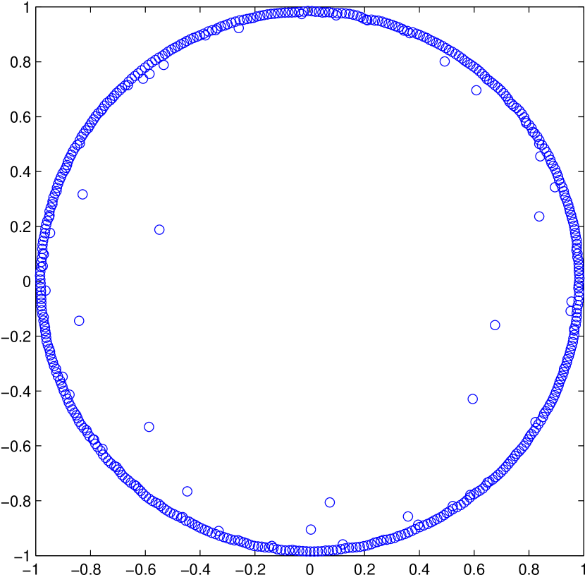
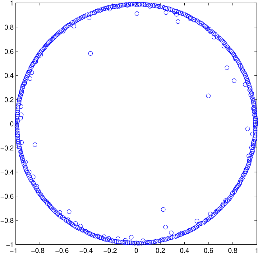
Figure 1. On the left hand side $\delta=10^{-5}$ and on the right hand side $\delta=10^{-4}$.

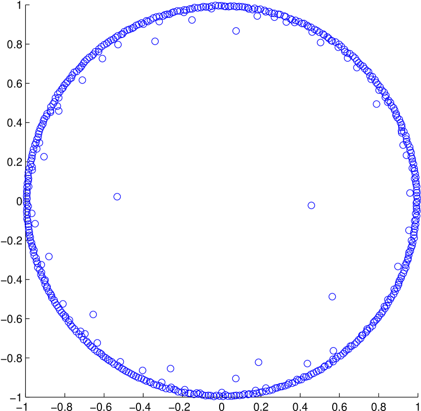
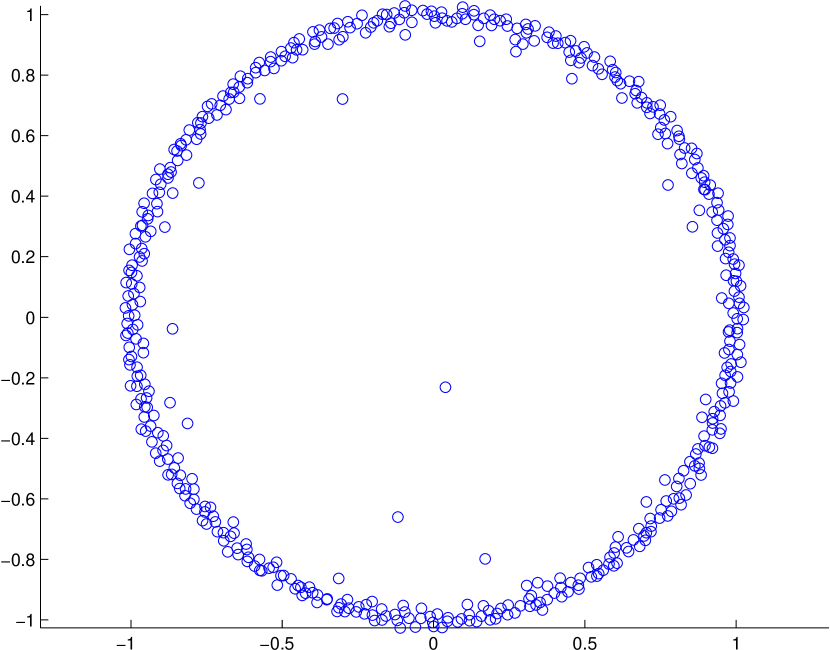
Figure 2. On the left hand side $\delta=10^{-3}$ and on the right hand side $\delta=10^{-2}$.

3. A general formula

To start with, we shall obtain a general formula (due to [20] in a similar context). Our treatment is slightly different in that we avoid the use of approximations of the delta function and also that we have more holomorphy available.

Let $g(z,Q)$ be a holomorphic function on $\Omega\times W\subset{\mathds{C}}\times{\mathds{C}}^{N^{2}}$, where $\Omega\subset\mathds{C}$, $W\subset{\mathds{C}}^{N^{2}}$ are open bounded and connected. Assume that

$$\hbox{for every }Q\in W,\ g(\cdot,Q)\not\equiv 0.$$ (3.1)

To start with, we also assume that

$$\hbox{for almost all }Q\in W,\ g(\cdot,Q)\hbox{ has only simple zeros.}$$ (3.2)

Let $\phi\in C_{0}^{\infty}(\Omega)$ and let $m\in C_{0}(W)$. We are interested in

$$K_{\phi}=\int\left(\sum_{z;\,g(z,Q)=0}\phi(z)\right)m(Q)L(dQ),$$ (3.3)

where we frequently identify the Lebesgue measure with a differential form,

$$L(dQ)\simeq(2i)^{-{N^{2}}}d\overline{Q}_{1}\wedge dQ_{1}\wedge...\wedge d\overline{Q}_{N^{2}}\wedge dQ_{N^{2}}=:(2i)^{-{N^{2}}}d\overline{Q}\wedge dQ.$$

In (3.3) we count the zeros of $g(\cdot,Q)$ with their multiplicity and notice that the integral is finite: For every compact set $K\subset W$ the number of zeros of $g(\cdot,Q)$ in $\mathrm{supp\,}\phi$, counted with their multiplicity, is uniformly bounded, for $Q\in K$. This follows from Jensen’s formula.

Now assume,

$$g(z,Q)=0\Rightarrow d_{Q}g\neq 0.$$ (3.4)

Then

$$\Sigma:=\{(z,Q)\in\Omega\times W;\,g(z,Q)=0\}$$

is a smooth complex hypersurface in $\Omega\times W$ and from (3.2) we see that

$$K_{\phi}=\int_{\Sigma}\phi(z)m(Q)(2i)^{-{N^{2}}}d\overline{Q}\wedge dQ,$$ (3.5)

where we view $(2i)^{-{N^{2}}}d\overline{Q}\wedge dQ$ as a complex $({N^{2}},{N^{2}})$-form on $\Omega\times W$, restricted to $\Sigma$, which yields a non-negative differential form of maximal degree on $\Sigma$.

Before continuing, let us eliminate the assumption (3.2). Without that assumption, the integral in (3.3) is still well-defined. It suffices to show (3.5) for all $\phi\in\mathcal{C}_{0}^{\infty}(\Omega_{0}\times W_{0})$ when $\Omega_{0}\times W_{0}$ is a sufficiently small open neighborhood of any given point $(z_{0},Q_{0})\in\Omega\times W$. When $g(z_{0},Q_{0})\neq 0$ or $\partial_{z}g(z_{0},\Omega_{0})\neq 0$ we already know that this holds, so we assume that for some $m\geq 2$, $\partial_{z}^{k}g(z_{0},Q_{0})=0$ for $0\leq k\leq m-1$, $\partial_{z}^{m}g(z_{0},Q_{0})\neq 0$.

Put $g_{\varepsilon}(z,Q)=g(z,Q)+\varepsilon$, $\varepsilon\in\mathrm{neigh}(0,\mathds{C})$. By Weierstrass’ preparation theorem, if $\Omega_{0},W_{0}$ and $r>0$ are small enough,

$$g_{\varepsilon}(z,Q)=k(z,Q,\varepsilon)p(z,Q,\varepsilon)\quad\text{in }\Omega_{0}\times W_{0}\times D(0,r),$$

where $k$ is holomorphic and non-vanishing, and

$$p(z,Q,\varepsilon)=z^{m}+p_{1}(Q,\varepsilon)z^{m-1}+\dots+p_{m}(Q,\varepsilon).$$

Here, $p_{j}(Q,\varepsilon)$ are holomorphic, and $p_{j}(0,0)=0$.

The discriminant $D(Q,\varepsilon)$ of the polynomial $p(\cdot,Q,\varepsilon)$ is holomorphic on $W_{0}\times D(0,r)$. It vanishes precisely when $p(\cdot,Q,\varepsilon)$ - or equivalently $g_{\varepsilon}(\cdot,Q)$ - has a multiple root in $\Omega_{0}$.

Now for $0<|\varepsilon|\ll 1$, the $m$ roots of $g_{\varepsilon}(\cdot,Q_{0})$ are simple, so $D(Q_{0},\varepsilon)\neq 0$. Thus, $D(\cdot,\varepsilon)$ is not identically zero, so the zero set of $D(\cdot,\varepsilon)$ in $W_{0}$ is of measure $0$ (assuming that we have chosen $W_{0}$ connected). This means that for $0<|\varepsilon|\ll 1$, the function $g_{\varepsilon}(\cdot,Q)$ has only simple roots in $\Omega$ for almost all $Q\in W_{0}$.

Let $\Sigma_{\epsilon}$ be the zero set of $g_{\epsilon}$, so that $\Sigma_{\epsilon}\to\Sigma$ in the natural sense. We have

$$\int\left(\sum_{z;\,g_{\epsilon}(z,Q)=0}\phi(z)\right)m(Q)(2i)^{-{N^{2}}}d\overline{Q}\wedge dQ=\int_{\Sigma_{\epsilon}}\phi(z)m(Q)(2i)^{-{N^{2}}}d\overline{Q}\wedge dQ$$

for $\phi\in\mathcal{C}_{0}^{\infty}(\Omega_{0}\times W_{0})$, when $\epsilon>0$ is small enough, depending on $\phi$, $m$. Passing to the limit $\epsilon=0$ we get (3.5) under the assumptions (3.1), (3.4), first for $\phi\in\mathcal{C}_{0}^{\infty}(\Omega_{0}\times W_{0})$, and then by partition of unity for all $\phi\in\mathcal{C}_{0}^{\infty}(\Omega\times W)$. Notice that the result remains valid if we replace $m(Q)$ by $m(Q)1_{B}(Q)$ where $B$ is a ball in $W$.

Now we strengthen the assumption (3.4) by assuming that we have a non-zero $Z(z)\in{\mathds{C}}^{N^{2}}$ depending smoothly on $z\in\Omega$ (the dependence will actually be holomorphic in the application below) such that

$$g(z,Q)=0\Rightarrow\left(\overline{Z}(z)\cdot\partial_{Q}\right)g(z,Q)\neq 0.$$ (3.6)

We have the corresponding orthogonal decomposition

$$Q=Q(\alpha)=\alpha_{1}\overline{Z}(z)+\alpha^{\prime},\quad\alpha^{\prime}\in\overline{Z}(z)^{\perp},\ \alpha_{1}\in\mathds{C},$$

and if we identify unitarily $\overline{Z}(z)^{\perp}$ with ${\mathds{C}}^{{N^{2}}-1}$ by means of an orthonormal basis $e_{2}(z),...,e_{N^{2}}(z)$, so that $\alpha^{\prime}=\sum_{2}^{N^{2}}\alpha_{j}e_{j}(z)$ we get global coordinates $\alpha_{1},\alpha_{2},...,\alpha_{N^{2}}$ on $Q$-space.

By the implicit function theorem, at least locally near any given point in $\Sigma$, we can represent $\Sigma$ by $\alpha_{1}=f(z,\alpha^{\prime})$, $\alpha^{\prime}\in\overline{Z}(z)^{\perp}\simeq{\mathds{C}}^{{N^{2}}-1}$, where $f$ is smooth. (In the specific situation below, this will be valid globally.) Clearly, since $z,\alpha_{2},...,\alpha_{N^{2}}$ are complex coordinates on $\Sigma$, we have on $\Sigma$ that

$$\frac{1}{(2i)^{N^{2}}}d\overline{Q}\wedge dQ=J(f)\frac{d\overline{z}\wedge dz}{2i}(2i)^{1-N^{2}}d\overline{\alpha}_{2}\wedge d\alpha_{2}\wedge...\wedge d\overline{\alpha}_{N^{2}}\wedge d\alpha_{N^{2}}$$

with the convention that

$$J(f)\frac{d\overline{z}\wedge dz}{2i}\geq 0,\quad(2i)^{1-N^{2}}d\overline{\alpha}_{2}\wedge d\alpha_{2}\wedge...\wedge d\overline{\alpha}_{N^{2}}\wedge d\alpha_{N^{2}}>0.$$

Thus

$$\begin{split}K_{\phi}=\int\phi(z)m\left(f(z,\alpha^{\prime})\overline{Z}(z)+\alpha^{\prime}\right)J(f)(z,\alpha_{2},...,\alpha_{N^{2}})\times\\ (2i)^{-{N^{2}}}d\overline{z}\wedge dz\wedge d\overline{\alpha}_{2}\wedge d\alpha_{2}\wedge...\wedge d\overline{\alpha}_{N^{2}}\wedge d\alpha_{N^{2}}.\end{split}$$ (3.7)

The Jacobian $J(f)$ is invariant under any $z$-dependent unitary change of variables, $\alpha_{2},...,\alpha_{N^{2}}\mapsto\widetilde{\alpha}_{2},...,\widetilde{\alpha}_{N^{2}}$, so for the calculation of $J(f)$ at a given point $(z_{0},\alpha_{0}^{\prime})$, we are free to choose the most appropriate orthonormal basis $e_{2}(z),...,e_{N^{2}}(z)$ in $\overline{Z}(z)^{\perp}$ depending smoothly on $z$. We write (3.7) as

$$K_{\phi}=\int\phi(z)\Xi(z)\frac{d\overline{z}\wedge dz}{2i},$$ (3.8)

where the density $\Xi(z)$ is given by

$$\begin{split}\Xi(z)=\int_{\alpha^{\prime}=\sum_{2}^{N^{2}}\alpha_{j}e_{j}(z)}m(f(z,\alpha^{\prime})\overline{Z}(z)+\alpha^{\prime})J(f)(z,\alpha_{2},...,\alpha_{N^{2}})\times\\ (2i)^{1-{N^{2}}}d\overline{\alpha}_{2}\wedge d\alpha_{2}\wedge...\wedge d\overline{\alpha}_{N^{2}}\wedge d\alpha_{N^{2}}.\end{split}$$ (3.9)

Before continuing, let us give a brief overview on the organization of following sections:

In Section 4 we will set up an auxiliary Grushin problem yielding the effective function $g$ as above. Section 5 deals with the appropriate choice of coordinates $Q$ and the calculation of the Jacobian $J(f)$. Finally, in Section 6 we complete the proof of Theorem 2.2.

4. Grushin problem for the perturbed Jordan block

4.1. Setting up an auxiliary problem

Following [16], we introduce an auxiliary Grushin problem. Define $R_{+}:{\mathds{C}}^{N}\to{\mathds{C}}$ by

$$R_{+}u=u_{1},\ u=(u_{1}\ ...\ u_{N})^{\mathrm{t}}\in{\mathds{C}}^{N}.$$ (4.1)

Let $R_{-}:\,{\mathds{C}}\to{\mathds{C}}^{N}$ be defined by

$$R_{-}u_{-}=(0\ 0\ ...\ u_{-})^{\mathrm{t}}\in{\mathds{C}}^{N}.$$ (4.2)

Here, we identify vectors in ${\mathds{C}}^{N}$ with column matrices. Then for $|z|<1$, the operator

$${\mathcal{A}}_{0}=\begin{pmatrix}A_{0}-z&R_{-}\\ R_{+}&0\end{pmatrix}:{\mathds{C}}^{N+1}\to{\mathds{C}}^{N+1}$$ (4.3)

is bijective. In fact, identifying

$${\mathds{C}}^{N+1}\simeq\ell^{2}([1,2,...,N+1])\simeq\ell^{2}({\mathds{Z}}/(N+1){\mathds{Z}}),$$

we have ${\mathcal{A}}_{0}=\tau^{-1}-z\Pi_{N}$, where $\tau u(j)=u(j-1)$ (translation by 1 step to the right) and $\Pi_{N}u=1_{[1,N]}u$. Then ${\mathcal{A}}_{0}=\tau^{-1}(1-z\tau\Pi_{N})$, $(\tau\Pi_{N})^{N+1}=0$,

$${\mathcal{A}}_{0}^{-1}=(1+z\tau\Pi_{N}+(z\tau\Pi_{N})^{2}+...+(z\tau\Pi_{N})^{N})\circ\tau.$$

Write

$${\mathcal{E}}_{0}:={\mathcal{A}}_{0}^{-1}=:\begin{pmatrix}E^{0}&E_{+}^{0}\\ E_{-}^{0}&E_{-+}^{0}\end{pmatrix}.$$

Then

$$E^{0}\simeq\Pi_{N}(1+z\tau\Pi_{N}+...(z\tau\Pi_{N})^{N-1})\tau\Pi_{N},$$ (4.4)

$$E_{+}^{0}=\begin{pmatrix}1\\ z\\ ..\\ z^{N-1}\end{pmatrix},\ E_{-}^{0}=\begin{pmatrix}z^{N-1}&z^{N-2}&...&1\end{pmatrix},$$ (4.5)

$$E_{-+}^{0}=z^{N}.$$ (4.6)

A quick way to check (4.5), (4.6) is to write $\mathcal{A}_{0}$ as an $(N+1)\times(N+1)$-matrix where we moved the last line to the top, with the lines labeled from $0$ ($\equiv N+1\mod(N+1)\mathds{Z}$) to $N$ and the columns from $1$ to $N+1$.

Continuing, we see that

$$\|E^{0}\|\leq G(|z|),\ \|E_{\pm}^{0}\|\leq G(|z|)^{\frac{1}{2}},\ \|E_{-+}^{0}\|\leq 1,$$ (4.7)

where $\|\cdot\|$ denote the natural operator norms and

$$G(|z|):=\min\left(N,\frac{1}{1-|z|}\right)\asymp 1+|z|+|z|^{2}+...+|z|^{N-1}.$$ (4.8)

Next, consider the natural Grushin problem for $A_{\delta}$. If $\delta\|Q\|G(|z|)<1$, we see that

$${\mathcal{A}}_{\delta}=\begin{pmatrix}A_{\delta}-z&R_{-}\\ R_{+}&0\end{pmatrix}$$ (4.9)

is bijective with inverse

$${\mathcal{E}}_{\delta}=\begin{pmatrix}E^{\delta}&E_{+}^{\delta}\\ E_{+}^{\delta}&E_{-+}^{\delta}\end{pmatrix},$$

where

$$\begin{split}E^{\delta}=&E^{0}-E^{0}\delta QE^{0}+E^{0}(\delta QE^{0})^{2}-...=E^{0}(1+\delta QE^{0})^{-1},\\ E_{+}^{\delta}=&E_{+}^{0}-E^{0}\delta QE_{+}^{0}+(E^{0}\delta Q)^{2}E_{+}^{0}-...=(1+E^{0}\delta Q)^{-1}E^{0}_{+},\\ E_{-}^{\delta}=&E_{-}^{0}-E_{-}^{0}\delta QE^{0}+E_{-}^{0}(\delta QE^{0})^{2}-...=E_{-}^{0}(1+\delta QE^{0})^{-1},\\ E^{\delta}_{-+}=&E^{0}_{-+}-E_{-}^{0}\delta QE_{+}^{0}+E_{-}^{0}\delta QE^{0}\delta QE_{+}^{0}-...\\ &=E_{-+}^{0}-E_{-}^{0}\delta Q(1+E^{0}\delta Q)^{-1}E_{+}^{0}.\end{split}$$ (4.10)

We get

$$\begin{split}&\|E^{\delta}\|\leq\frac{G(|z|)}{1-\delta\|Q\|G(|z|)},\ \|E_{\pm}^{\delta}\|\leq\frac{G(|z|)^{\frac{1}{2}}}{1-\delta\|Q\|G(|z|)},\\ &|E_{-+}^{\delta}-E_{-+}^{0}|\leq\frac{\delta\|Q\|G(|z|)}{1-\delta\|Q\|G(|z|)}.\end{split}$$ (4.11)

Indicating derivatives with respect to $\delta$ with dots and omitting sometimes the super/sub-script $\delta$, we have

$$\dot{{\mathcal{E}}}=-{\mathcal{E}}\dot{{\mathcal{A}}}{\mathcal{E}}=-\begin{pmatrix}EQE&EQE_{+}\\ E_{-}QE&E_{-}QE_{+}.\end{pmatrix}$$ (4.12)

Integrating this from 0 to $\delta$ yields

$$\|E^{\delta}-E^{0}\|\leq\frac{G(|z|)^{2}\delta\|Q\|}{(1-\delta\|Q\|G(|z|))^{2}},\quad\|E_{\pm}^{\delta}-E_{\pm}^{0}\|\leq\frac{G(|z|)^{\frac{3}{2}}\delta\|Q\|}{(1-\delta\|Q\|G(|z|))^{2}}.$$ (4.13)

We now sharpen the assumption that $\delta\|Q\|G(|z|)<1$ to

$$\delta\|Q\|G(|z|)<1/2.$$ (4.14)

Then

$$\begin{split}&\|E^{\delta}\|\leq 2G(|z|),\ \|E_{\pm}^{\delta}\|\leq 2G(|z|)^{\frac{1}{2}},\\ &|E_{-+}^{\delta}-E_{-+}^{0}|\leq 2\delta\|Q\|G(|z|).\end{split}$$ (4.15)

Combining this with the identity $\dot{E}_{-+}=-E_{-}QE_{+}$ that follows from (4.12), we get

$$\|\dot{E}_{-+}+E_{-}^{0}QE_{+}^{0}\|\leq 16G(|z|)^{2}\delta\|Q\|^{2},$$ (4.16)

and after integration from $0$ to $\delta$,

$$E_{-+}^{\delta}=E_{-+}^{0}-\delta E_{-}^{0}QE_{+}^{0}+{\mathcal{O}}(1)G(|z|)^{2}(\delta\|Q\|)^{2}.$$ (4.17)

Using (4.5), (4.6) we get with $Q=(q_{j,k})$,

$$E_{-+}^{\delta}=z^{N}-\delta\sum_{j,k=1}^{N}q_{j,k}z^{N-j+k-1}+{\mathcal{O}}(1)G(|z|)^{2}(\delta\|Q\|)^{2},$$ (4.18)

still under the assumption (4.14).

4.2. Estimates for the effective Hamiltonian

We now consider the situation at the beginning of Section 2:

$$A_{\delta}=A_{0}+\delta Q,\ Q=(q_{j,k}(\omega))_{j,k=1}^{N},\ q_{j,k}(\omega)\sim{\mathcal{N}}_{\mathds{C}}(0,1)\hbox{ independent.}$$

In the following, we often write $|\cdot|$ for the Hilbert-Schmidt norm $\lVert\cdot\rVert_{\mathrm{HS}}$. As we recalled in (2.2), we have

$$|Q|\leq C_{1}N\hbox{ with probability }\geq 1-e^{-N^{2}},$$ (4.19)

and we shall work under the assumption that $|Q|\leq C_{1}N$. We let $|z|<1$ and assume:

$$\delta NG(|z|)\ll 1.$$ (4.20)

Then with probability $\geq 1-e^{-N^{2}}$, we have (4.14), (4.18) which give for $g(z,Q):=E_{-+}^{\delta}$,

$$g(z,Q)=z^{N}+\delta(Q|\overline{Z}(z))+{\mathcal{O}}(1)(G(|z|)\delta N)^{2}.$$ (4.21)

Here, $Z$ is given by

$$Z=\left(z^{N-j+k-1}\right)_{j,k=1}^{N}.$$ (4.22)

A straight forward calculation shows that

$$|Z|=\sum_{0}^{N-1}|z|^{2\nu}=\frac{1-|z|^{2N}}{1-|z|^{2}}=\frac{1-|z|^{N}}{1-|z|}\,\,\frac{1+|z|^{N}}{1+|z|},$$ (4.23)

and in particular,

$$\frac{G(|z|)}{2}\leq|Z|\leq G(|z|).$$ (4.24)

The middle term in (4.21) is bounded in modulus by $\delta|Q||Z|\leq\delta C_{1}NG(|z|)$ and we assume that $|z|^{N}$ is much smaller than this bound:

$$|z|^{N}\ll\delta C_{1}NG(|z|).$$ (4.25)

More precisely, we work in a disc $D(0,r_{0})$, where

$$r_{0}^{N}\leq C^{-1}\delta C_{1}NG(r_{0})\leq C^{-2},\quad r_{0}\leq 1-N^{-1}$$ (4.26)

and $C\gg 1$. In fact, the first inequality in (4.26) can be written $m(r_{0})\leq C^{-1}\delta C_{1}N$ and $m(r)=r^{N}(1-r)$ is increasing on $[0,1-N^{-1}]$ so the inequality is preserved if we replace $r_{0}$ by $|z|\leq r_{0}$. Similarly, the second inequality holds after the same replacement since $G$ is increasing.

In view of (4.20), we see that

$$\left(G(|z|)\delta N\right)^{2}\ll\delta G(|z|)N$$

is also much smaller than the upper bound on the middle term.

By the Cauchy inequalities,

$$d_{Q}g=\delta Z\cdot dQ+{\mathcal{O}}(1)G(|z|)^{2}\delta^{2}N.$$ (4.27)

The norm of the first term is $\asymp\delta G\gg G^{2}\delta^{2}N$, since $G\delta N\ll 1$. (When applying the Cauchy inequalities, we should shrink the radius $R=C_{1}N$ by a factor $\theta<1$, but we have room for that, if we let $C_{1}$ be a little larger than necessary to start with.)

Writing

$$Q=\alpha_{1}\overline{Z}(z)+\alpha^{\prime},\ \alpha^{\prime}\in\overline{Z}(z)^{\perp}\simeq{\mathds{C}}^{{N^{2}}-1},$$

we identify $g(z,Q)$ with a function $\widetilde{g}(z,\alpha)$ which is holomorphic in $\alpha$ for every fixed $z$ and satisfies

$$\widetilde{g}(z,\alpha)=z^{N}+\delta|Z(z)|^{2}\alpha_{1}+{\mathcal{O}}(1)G(|z|)^{2}\delta^{2}N^{2},$$ (4.28)

while (4.27) gives

$$\partial_{\alpha_{1}}\widetilde{g}(z,\alpha)=\delta|Z(z)|^{2}+{\mathcal{O}}(1)G(|z|)^{3}\delta^{2}N,$$ (4.29)

and in particular,

$$\left|\partial_{\alpha_{1}}\widetilde{g}\right|\asymp\delta G(|z|)^{2}.$$

This derivative does not depend on the choice of unitary identification $\overline{Z}^{\perp}\simeq{\mathds{C}}^{{N^{2}}-1}$. Notice that the remainder in (4.28) is the same as in (4.21) and hence a holomorphic function of $(z,Q)$. In particular it is a holomorphic function of $\alpha_{1},...,\alpha_{N^{2}}$ for every fixed $z$ and we can also get (4.29) from this and the Cauchy inequalities. In the same way, we get from (4.28) that

$$\partial_{\alpha_{j}}\widetilde{g}(z,\alpha)={\mathcal{O}}(1)G(|z|)^{2}\delta^{2}N,\ j=2,...,{N^{2}}.$$ (4.30)

The Cauchy inequalities applied to (4.21) give,

$$\partial_{z}g(z,Q)=Nz^{N-1}+\delta Q\cdot\partial_{z}Z(z)+{\mathcal{O}}(1)\frac{(G(|z|)\delta N)^{2}}{r_{0}-|z|}.$$ (4.31)

Then, for $\widetilde{g}(z,\alpha_{1},\alpha^{\prime})=g(z,\alpha_{1}\overline{Z}(z)+\alpha^{\prime})$, $\alpha^{\prime}=\sum_{2}^{N^{2}}\alpha_{j}e_{j}$ we shall see that

$$\begin{split}\partial_{z}\widetilde{g}=Nz^{N-1}+\delta\alpha_{1}\partial_{z}\left(|Z|^{2}\right)+{\mathcal{O}}(1)\frac{(G\delta N)^{2}}{r_{0}-|z|}+{\mathcal{O}}(1)G^{2}\delta^{2}N\left|\sum_{2}^{N^{2}}\alpha_{j}\partial_{z}e_{j}\right|,\end{split}$$ (4.32)

$$\begin{split}\partial_{\overline{z}}\widetilde{g}=&\delta\alpha_{1}\partial_{\overline{z}}\left(|Z|^{2}\right)+{\mathcal{O}}(1)G^{2}\delta^{2}N\left|\alpha_{1}\overline{\partial_{z}Z}+\sum_{2}^{N^{2}}\alpha_{j}\partial_{\overline{z}}e_{j}\right|.\end{split}$$ (4.33)

The leading terms in (4.32), (4.33) can be obtained formally from (4.28) by applying $\partial_{z}$, $\partial_{\overline{z}}$ and we also notice that

$$\partial_{z}|Z|^{2}=\overline{Z}\cdot\partial_{z}Z,\ \ \partial_{\overline{z}}|Z|^{2}=Z\cdot\overline{\partial_{z}Z}.$$

However it is not clear how to handle the remainder in (4.28), so we verify (4.32), (4.33), using (4.27), (4.31):

$$\begin{split}&\partial_{z}\widetilde{g}=\partial_{z}g+d_{Q}g\cdot\sum_{2}^{N^{2}}\alpha_{j}\partial_{z}e_{j}=\\ &Nz^{N-1}+\delta Q\cdot\partial_{z}Z+{\mathcal{O}}(1)\frac{(G\delta N)^{2}}{r_{0}-|z|}+(\delta Z\cdot dQ+{\mathcal{O}}(1)G^{2}\delta^{2}N)\cdot\sum_{2}^{N^{2}}\alpha_{j}\partial_{z}e_{j}\\ &=Nz^{N-1}+\delta\alpha_{1}\partial_{z}\left(|Z|^{2}\right)+\delta\sum_{2}^{N^{2}}\alpha_{j}e_{j}\cdot\partial_{z}Z+\delta Z\cdot\sum_{2}^{N^{2}}\alpha_{j}\partial_{z}e_{j}\\ &\hskip 142.26378pt+\hbox{ the remainders in (\ref{ed.27})}.\end{split}$$

The 3d and the 4th terms in the last expression add up to

$$\delta\partial_{z}\left(\sum_{2}^{N^{2}}\alpha_{j}e_{j}\cdot Z\right)=\delta\partial_{z}(0)=0,$$

and we get (4.32).

Similarly,

$$\begin{split}&\partial_{\overline{z}}\widetilde{g}=d_{Q}g\cdot\left(\alpha_{1}\overline{\partial_{z}Z}+\sum_{2}^{N^{2}}\alpha_{j}\partial_{\overline{z}}e_{j}\right)\\ &=\left(\delta Z\cdot dQ+{\mathcal{O}}(1)G^{2}\delta^{2}N\right)\cdot\left(\alpha_{1}\overline{\partial_{z}Z}+\sum_{2}^{N^{2}}\alpha_{j}\partial_{\overline{z}}e_{j}\right).\end{split}$$

Up to remainders as in (4.33), this is equal to

$$\delta\alpha_{1}Z\cdot\overline{\partial_{z}Z}+\delta\sum_{2}^{N^{2}}\alpha_{j}Z\cdot\partial_{\overline{z}}e_{j} =\delta\alpha_{1}\partial_{\overline{z}}\left(|Z|^{2}\right)+\delta\sum_{2}^{N^{2}}\alpha_{j}\partial_{\overline{z}}\left(Z\cdot e_{j}\right)$$

$$=\delta\alpha_{1}\partial_{\overline{z}}\left(|Z|^{2}\right).$$

Here, we know that

$$|Z(z)|=\sum_{0}^{N-1}(z\overline{z})^{\nu}=:K(z\overline{z}),$$

$$\begin{split}\partial_{z}\left(|Z(z)|^{2}\right)&=2KK^{\prime}\overline{z},\\ \partial_{\overline{z}}\left(|Z(z)|^{2}\right)&=2KK^{\prime}z.\end{split}$$ (4.34)

Observe also that $K(t)\asymp G(t)$ and that $G(|z|)\asymp G(|z|^{2})$.

The following result implies that $K^{\prime}(t)$ and $K(t)^{2}$ are of the same order of magnitude.

Proposition 4.1.

For $k\in{\mathds{N}}$, $2\leq N\in{\mathds{N}}\cup\{+\infty\}$, $0\leq t<1$, we put

$$M_{N,k}(t)=\sum_{\nu=1}^{N-1}\nu^{k}t^{\nu},$$ (4.35)

so that $K(t)=K_{N}(t)=M_{N,0}(t)+1$, $K^{\prime}(t)\asymp M_{N-1,1}(t)+1$. For each fixed $k\in{\mathds{N}}$, we have uniformly with respect to $N$, $t$:

$$M_{\infty,k}(t)\asymp\frac{t}{(1-t)^{k+1}},$$ (4.36)

$$M_{\infty,k}(t)-M_{N,k}(t)\asymp\frac{t^{N}}{1-t}\left(N+\frac{1}{1-t}\right)^{k}.$$ (4.37)

For all fixed $C>0$ and $k\in{\mathds{N}}$, we have uniformly,

$$M_{N,k}(t)\asymp M_{\infty,k}(t),\hbox{ for }0\leq t\leq 1-\frac{1}{CN},\ N\geq 2.$$ (4.38)

Notice that under the assumption in (4.38), the estimate (4.37) becomes

$$M_{\infty,k}(t)-M_{N,k}(t)\asymp\frac{t^{N}N^{k}}{1-t}.$$

We also see that in any region $1-{\mathcal{O}}(1)/N\leq t<1$, we have

$$M_{N,k}(t)\asymp N^{k+1},$$

so together with (4.38), (4.36), this shows that

$$M_{N,k}(t)\asymp t\min\left(\frac{1}{1-t},N\right)^{k+1}.$$ (4.39)

Proof.

The statements are easy to verify when $0\leq t\leq 1-1/{\mathcal{O}}(1)$ and the $N$-dependent statements (4.37), (4.38) are clearly true when $N\leq{\mathcal{O}}(1)$. Thus we can assume that $1/2\leq t<1$ and $N\gg 1$.

Write $t=e^{-s}$ so that $0<s\leq 1/{\mathcal{O}}(1)$ and notice that $s\asymp 1-t$. For $N\in{\mathds{N}}$, we put

$$P_{N,k}(s)=\sum_{\nu=N}^{\infty}\nu^{k}e^{-\nu s},$$ (4.40)

so that

$$P_{N,k}(s)=\begin{cases}M_{\infty,k}(t)\hbox{ when }N=1,\\ M_{\infty,k}(t)-M_{N,k}(t)\hbox{ when }N\geq 2.\end{cases}$$ (4.41)

We regroup the terms in (4.40) into sums with $\asymp 1/s$ terms where $e^{-\nu s}$ has constant order of magnitude:

$$P_{N,k}(s)=\sum_{\mu=1}^{\infty}\Sigma(\mu),\quad\Sigma(\mu)=\sum_{N+\frac{\mu-1}{s}\leq\nu<N+\frac{\mu}{s}}\nu^{k}e^{-\nu s}.$$

Here, since the sum $\Sigma(\mu)$ consists of $\asymp 1/s$ terms of the order $\nu^{k}e^{-(Ns+\mu)}$,

$$\Sigma(\mu)\asymp e^{-(Ns+\mu)}\sum_{N+\frac{\mu-1}{s}\leq\nu<N+\frac{\mu}{s}}\nu^{k}\asymp e^{-(Ns+\mu)}\frac{(Ns+\mu)^{k}}{s^{k+1}}.$$

Hence,

$$\begin{split}P_{N,k}(s)&\asymp\frac{e^{-Ns}}{s^{k+1}}\sum_{\mu=1}^{\infty}e^{-\mu}(Ns+\mu)^{k}\\ &\asymp\frac{e^{-Ns}}{s^{k+1}}(Ns+1)^{k}=\frac{e^{-Ns}}{s}\left(N+\frac{1}{s}\right)^{k}.\end{split}$$

Recalling (4.41) and the fact that $s\asymp 1-t$, $1/2\leq t<1$, we get (4.36) when $N=1$ and (4.37) when $N\geq 2$.

It remains to show (4.38) and it suffices to do so for $1/2\leq t\leq 1-C/N$, $N\gg 1$ and for $C\geq 1$ sufficiently large but independent of $N$. Indeed, for $1-C/N\leq t\leq 1-1/{\mathcal{O}}(N)$, both $M_{N,k}(t)$ and $M_{\infty,k}(t)$ are $\asymp N^{1+k}$. We can also exclude the case $k=0$ where we have explicit formulae.

To get the equivalence (4.38) for $1/2\leq t\leq 1-C/N$, $k\geq 1$, it suffices, in view of (4.36), (4.37), to show that for such $t$ and for $N\gg 1$, we have

$$\frac{N^{k}t^{N}}{1-t}\leq\frac{1}{D}\frac{1}{(1-t)^{k+1}},$$

for any given $D\geq 1$, provided that $C$ is large enough. In other terms, we need

$$t^{N}(1-t)^{k}\leq\frac{1}{D}N^{-k},\hbox{ for }\frac{1}{2}\leq t\leq 1-\frac{C}{N},$$

when $C=C(D)$ is large enough and $N\geq N(C)\gg 1$. The left hand side in this inequality is an increasing function of $t$ on the interval $[0,1/\left(1+k/N\right)]$. If $t\leq 1-C/N\leq 1/(1+k/N)$ (which is fulfilled when $C\geq 2k$ and $N\gg N(C)$) it is

$$\leq\left(1-\frac{C}{N}\right)^{N}\left(\frac{C}{N}\right)^{k}=\left(1+{\mathcal{O}}_{C}\left(\frac{1}{N}\right)\right)e^{-C}C^{k}N^{-k}.$$

This is $\leq N^{-k}/D$ if $C\geq C(D)$, $N\geq N(C)$. ∎

For simplicity we will restrict the attention to the region

$$|z|\leq r_{0}-1/N,$$ (4.42)

where $G\asymp(1-|z|)^{-1}$, $G^{\prime}\asymp(1-|z|)^{-2}$.

It follows from the calculation (5.6) below, that

$$|\partial_{z}Z|^{2}=\left(\frac{2}{t}\left(K(t\partial_{t})^{2}K+(t\partial_{t}K)^{2}\right)\right)_{t=|z|^{2}}.$$

This is $\asymp 1$ for $|z|\leq 1/2$ and for $1/2\leq|z|<1-1/N$ it is in view of Proposition 4.1 and the subsequent observation

$$\asymp M_{N,0}M_{N,2}+M_{N,1}^{2}\asymp\frac{1}{(1-t)^{4}},\ t=|z|^{2}.$$

In the region (4.42) we get:

$$|Z^{\prime}(z)|\asymp G(|z|)^{2}.$$ (4.43)

(4.34), (4.42), (4.43) will be used in (4.32), (4.33).

Combining the implicit function theorem and Rouché’s theorem to (4.28),we see that for $|\alpha^{\prime}|<C_{1}N$, $\alpha^{\prime}=\sum_{2}^{N}\alpha_{j}e_{j}\in\overline{Z}(z)^{\perp}$, the equation

$$\widetilde{g}(z,\alpha_{1},\alpha^{\prime})=0$$ (4.44)

has a unique solution

$$\alpha_{1}=f(z,\alpha^{\prime})\in D(0,C_{1}N/G(|z|)).$$ (4.45)

Here, we also use (4.20), (4.25). Moreover, $f$ satisfies

$$f(z,\alpha^{\prime})=-\frac{z^{N}}{\delta|Z|^{2}}+{\mathcal{O}}(1)\delta N^{2}={\mathcal{O}}(1)\left(\frac{|z|^{N}}{\delta G^{2}}+\delta N^{2}\right).$$ (4.46)

Differentiating the equation (4.44) (where $\alpha_{1}=f$) we get

$$\partial_{z}\widetilde{g}+\partial_{\alpha}\widetilde{g}\partial_{z}f=0,\ \partial_{\overline{z}}\widetilde{g}+\partial_{\alpha}\widetilde{g}\partial_{\overline{z}}f=0.$$

Hence,

$$\begin{cases}\partial_{z}f=-\left(\partial_{\alpha_{1}}\widetilde{g}\right)^{-1}\partial_{z}\widetilde{g},\\ \partial_{\overline{z}}f=-\left(\partial_{\alpha_{1}}\widetilde{g}\right)^{-1}\partial_{\overline{z}}\widetilde{g}.\end{cases}$$ (4.47)

Since $\widetilde{g}$ is holomorphic in $\alpha_{1},\alpha^{\prime}$ and in $\alpha_{1},\alpha_{2},...,\alpha_{N^{2}}$, we see that $f$ is holomorphic in $\alpha^{\prime}$ and in $\alpha_{2},...,\alpha_{N^{2}}$ Applying $\partial_{\alpha_{2}},...,\partial_{\alpha_{N^{2}}}$ to (4.44), we get

$$\partial_{\alpha_{j}}f=-\left(\partial_{\alpha_{1}}\widetilde{g}\right)^{-1}\partial_{\alpha_{j}}\widetilde{g},\ 2\leq j\leq{N^{2}}.$$ (4.48)

Combining (4.29) in the form,

$$\partial_{\alpha_{1}}\widetilde{g}(z,\alpha)=(1+{\mathcal{O}}(G(|z|)\delta N))\delta|Z(z)|^{2},$$

(4.30), (4.32), (4.33) with (4.47) and (4.48), we get

$$\begin{split}&\partial_{z}f=-\frac{(1+{\mathcal{O}}(G\delta N))}{\delta|Z(z)|^{2}}\times\\ &\left(Nz^{N-1}+\delta f\partial_{z}\left(|Z|^{2}\right)+{\mathcal{O}}\left(G^{2}\delta^{2}N\right)\left|\sum_{2}^{N^{2}}\alpha_{j}\partial_{z}e_{j}\right|+{\mathcal{O}}(1)\frac{(G\delta N)^{2}}{r_{0}-|z|}\right).\end{split}$$ (4.49)

$$\begin{split}\partial_{\overline{z}}f=&-\frac{(1+{\mathcal{O}}(G\delta N))}{\delta|Z(z)|^{2}}\times\\ &\left(\delta f\partial_{\overline{z}}\left(|Z|^{2}\right)+{\mathcal{O}}\left(G^{2}\delta^{2}N\right)\left|f\overline{\partial_{z}Z}+\sum_{2}^{N^{2}}\alpha_{j}\partial_{\overline{z}}e_{j}\right|\right),\end{split}$$ (4.50)

$$\partial_{\alpha_{j}}f={\mathcal{O}}(1)\frac{G^{2}\delta^{2}N}{\delta G^{2}}={\mathcal{O}}(\delta N),\ 2\leq j\leq{N^{2}}.$$ (4.51)

From (4.34) and the observation prior to Proposition 4.1 we know that

$$\partial_{z}\left(|Z|^{2}\right),\ \partial_{\overline{z}}\left(|Z|^{2}\right)\asymp G(|z|)^{3}|z|.$$

Recall also that $|Z|\asymp G(|z|)$. Using this in (4.49), (4.50), we get

$$\begin{split}\partial_{z}f=&\frac{{\mathcal{O}}(1)}{\delta G^{2}}\times\\ &\left(N|z|^{N-1}+\delta|f|G^{3}|z|+{\mathcal{O}}\left(G^{2}\delta^{2}N\right)\left|\sum_{2}^{N^{2}}\alpha_{j}\partial_{z}e_{j}\right|+{\mathcal{O}}(1)\frac{G^{2}\delta^{2}N^{2}}{r_{0}-|z|})\right).\end{split}$$ (4.52)

5. Choosing appropriate coordinates

The next task will be to choose an orthonormal basis $e_{1}(z),e_{2},...,e_{N^{2}}(z)$ in ${\mathds{C}}^{N^{2}}$ with $e_{1}(z)=|Z(z)|^{-1}\overline{Z}(z)$ such that we get a nice control over $\sum_{2}^{N^{2}}\alpha_{j}\partial_{z}e_{j}$, $\sum_{2}^{N^{2}}\alpha_{j}\partial_{\overline{z}}e_{j}$ and such that

$${{dQ_{1}\wedge...\wedge dQ_{N^{2}}}_{|}}_{\alpha_{1}=f(z,\alpha^{\prime})}$$

can be expressed easily up to small errors. Consider a point $z_{0}\in D(0,r_{0}-N^{-1})$. We shall see below that the vectors $\overline{Z}(z)$, $\overline{\partial_{z}Z}(z)$ are linearly independent for every $z\in D(0,1)$

Proposition 5.1.

There exists an orthonormal basis $e_{1}(z),e_{2}(z),...,e_{N^{2}}(z)$ in ${\mathds{C}}^{N^{2}}$, depending smoothly on $z\in\mathrm{neigh\,}(z_{0})$ such that

$$e_{1}(z)=|Z(z)|^{-1}\overline{Z}(z),$$ (5.1)

$${\mathds{C}}e_{1}(z_{0})\oplus{\mathds{C}}e_{2}(z_{0})={\mathds{C}}\overline{Z}(z_{0})\oplus\overline{\partial_{z}Z}(z_{0}),$$ (5.2)

$$e_{j}(z)-e_{j}(z_{0})={\mathcal{O}}((z-z_{0})^{2}),\ j\geq 3.$$ (5.3)

Proof.

We choose $e_{1}(z)$ as in (5.1). Let $e_{3}(z_{0}),...,e_{N^{2}}(z_{0})$ be an orthonormal basis in $\left({\mathds{C}}\overline{Z}(z_{0})\oplus{\mathds{C}}\overline{\partial_{z}Z}(z_{0})\right)^{\perp}$. Then we get an orthonormal family $e_{3}(z),...,e_{N^{2}}(z)$ in $e_{1}(z)^{\perp}$ in the following way:

Let $V_{0}$ be the isometry ${\mathds{C}}^{{N^{2}}-2}\to{\mathds{C}}^{N^{2}}$, defined by $V_{0}\nu_{j}^{0}=e_{j}(z_{0})$, $j=3,...,{N^{2}}$, where $\nu_{3}^{0},...,\nu_{N^{2}}^{0}$ is the canonical basis in ${\mathds{C}}^{{N^{2}}-2}$ with a non-canonical labeling. Let $\pi(z)u=(u|e_{1}(z))e_{1}(z)$ be the orthogonal projection onto ${\mathds{C}}e_{1}(z)$. For $z\in\mathrm{neigh\,}(z_{0},{\mathds{C}})$, let $V(z)=(1-\pi(z))V_{0}$. Then $f_{j}(z)=V(z)\nu_{j}^{0}$, $j=3,...,{{N^{2}}}$ form a linearly independent system in $e_{1}(z)^{\perp}$ and we get an orthonormal system of vectors that span the same hyperplane in $e_{1}(z)^{\perp}$ by Gram orthonormalization,

$$e_{j}(z)=V(z)(V^{*}(z)V(z))^{-\frac{1}{2}}\nu_{j}^{0},\ 3\leq j\leq{N^{2}}.$$

We have

$$V(z)\nu_{j}^{0}=(1-\pi(z))e_{j}(z_{0})=e_{j}(z_{0})-(e_{j}(z_{0})|e_{1}(z))e_{1}(z),$$

$$(e_{j}(z_{0})|e_{1}(z))=\frac{(e_{j}(z_{0})|\overline{Z}(z))}{|Z(z)|}={\mathcal{O}}((z-z_{0})^{2}),$$

since $(e_{j}(z_{0})|\overline{Z}(z))=e_{j}(z_{0})\cdot Z(z)=:k(z)$ is a holomorphic function of $z$ with $k(z_{0})=(e_{j}(z_{0})|\overline{Z}(z_{0}))=0$, $k^{\prime}(z_{0})=(e_{j}(z_{0})|\overline{\partial_{z}Z}(z_{0}))=0$. Thus, $V(z)=V(z_{0})+{\mathcal{O}}(z-z_{0})^{2})$ and we conclude that (5.3) holds. Let $e_{2}(z)$ be a normalized vector in $(e_{1}(z),e_{3}(z),e_{4}(z),...,e_{N^{2}}(z))^{\perp}$ depending smoothly on $z$. Then $e_{1}(z),e_{2}(z),...,e_{N^{2}}(z)$ is an orthonormal basis and since $e_{3}(z_{0}),...,e_{N^{2}}(z_{0})$ are orthogonal to $\overline{Z}(z_{0}),\overline{\partial Z}(z_{0})$ by construction, we get (5.2). ∎

We can make the following explicit choice:

$$e_{2}(z)=|f_{2}|^{-1}f_{2},\ f_{2}=\overline{\partial_{z}Z}(z)-\sum_{j\neq 2}(\overline{\partial_{z}Z}(z)|e_{j}(z))e_{j}(z),$$ (5.4)

so that for $z=z_{0}$,

$$e_{2}(z_{0})=|f_{2}(z_{0})|^{-1}f_{2}(z_{0}),\ f_{2}(z_{0})=\overline{\partial_{z}Z}(z_{0})-(\overline{\partial_{z}Z}(z_{0})|e_{1}(z_{0}))e_{1}(z_{0}).$$ (5.5)

We next compute some scalar products and norms with $Z$ and $\partial_{z}Z$. Recall that $Z(z)=\left(z^{N-j+k-1}\right)_{j,k=1}^{N}$ and that $|Z(z)|=K(|z|^{2})$, $K(t)=\sum_{0}^{N-1}t^{\nu}$. Repeating basically the same computation, we get

$$z\partial_{z}Z=\left((N-j+k-1)z^{N-j+k-1}\right)_{j,k=1}^{N},$$

and

$$\begin{split}&|z\partial_{z}Z|^{2}=\sum_{j,k=1}^{N}(N-j+k-1)^{2}|z|^{2(N-j+k-1)}=\sum_{\nu,\mu=0}^{N-1}(\nu+\mu)^{2}|z|^{2(\nu+\mu)}\\ &=\sum_{0}^{N-1}\nu^{2}|z|^{2\nu}\sum_{0}^{N-1}|z|^{2\mu}+2\sum_{0}^{N-1}\nu|z|^{2\nu}\sum_{0}^{N-1}\mu|z|^{2\mu}+\sum_{0}^{N-1}|z|^{2\nu}\sum_{0}^{N-1}\mu^{2}|z|^{2\mu}\\ &=2\left(K(t\partial_{t})^{2}K+(t\partial_{t}K)^{2}\right)_{t=|z|^{2}}.\end{split}$$ (5.6)

Similarly,

$$\begin{split}(z\partial_{z}Z|Z)=&\sum_{j,k=1}^{N}(N-j+k-1)|z|^{2(N-j+k-1)}\\ =&\sum_{\nu=0}^{N-1}\sum_{\mu=1}^{N-1}(\nu+\mu)|z|^{2(\nu+\mu)}\\ =&2(Kt\partial_{t}K)_{t=|z|^{2}}.\end{split}$$

Then, by a straight forward calculation,

$$|\partial_{z}Z|^{2}-\frac{|(\partial_{z}Z|Z)|^{2}}{|Z|^{2}}=\left(\frac{2}{t}\left(K(t\partial_{t})^{2}K-(t\partial_{t}K)^{2}\right)\right)_{t=|z|^{2}}$$ (5.7)

Here,

$$\begin{split}\frac{2}{t}\left(K(t\partial_{t})^{2}K-(t\partial_{t}K)^{2}\right)&=\frac{2}{t}\sum_{0}^{N-1}t^{\nu}\sum_{0}^{N-1}\nu^{2}t^{\nu}-\frac{2}{t}\left(\sum_{0}^{N-1}\nu t^{\nu}\right)^{2}\\ =\sum_{\nu,\mu=0}^{N-1}\left(\nu^{2}+\mu^{2}-2\nu\mu\right)t^{\nu+\mu-1}&=\sum_{\nu,\mu=0}^{N-1}(\nu-\mu)^{2}t^{\nu+\mu-1}\\ &=\sum_{k=0}^{2N-3}a_{k,N}t^{k},\end{split}$$

where

$$a_{k,N}=\sum_{\begin{subarray}{c}\nu+\mu-1=k\\ 0\leq\nu,\mu\leq N-1\end{subarray}}(\nu-\mu)^{2}.$$

We observe that

$$a_{k,N}\leq{\mathcal{O}}(1)(1+k)^{3}\hbox{ uniformly with respect to }N,$$

$$a_{k,N}=a_{k,\infty}\hbox{ is independent of }N\hbox{ for }k\leq N-2,$$

$$a_{k,\infty}\geq(1+k)^{3}/{\mathcal{O}}(1).$$

We conclude that

$$\frac{1}{C}\left(1+M_{N-1,3}\right)\leq\frac{2}{t}\left(K(t\partial_{t})^{2}K-(t\partial_{t}K)^{2}\right)\leq C\left(1+M_{2N-2,3}\right)$$

and (4.39) shows that the first and third members are of the same order of magnitude,

$$\asymp 1+M_{N,3}(t)\asymp\min\left(\frac{1}{1-t},N\right)^{4}$$

which is $\asymp 1+M_{\infty,3}(t)$, for $0\leq t\leq 1-1/N$. From this and Proposition 4.1 we get:

Proposition 5.2.

We have

$$\frac{2}{t}(K(t\partial_{t})^{2}K-(t\partial_{t}K)^{2})\asymp K^{4},\ 0<t\leq 1-1/N,$$ (5.8)

where we recall that $K=K_{N}$ depends on $N$ and that

$$K_{N}=K_{\infty}-\frac{t^{N}}{1-t}.$$

We have

$$\begin{cases}t\partial_{t}K_{N}=t\partial_{t}K_{\infty}+{\mathcal{O}}\left(\frac{Nt^{N}}{1-t}\right),\ &t\leq 1-\frac{1}{N},\\ (t\partial_{t})^{2}K_{N}=(t\partial_{t})^{2}K_{\infty}+{\mathcal{O}}\left(\frac{N^{2}t^{N}}{1-t}\right),\ &t\leq 1-\frac{1}{N},\end{cases}$$ (5.9)

and it follows that

$$\frac{2}{t}\left(K_{N}(t\partial_{t})^{2}K_{N}-(t\partial_{t}K_{N})^{2}\right)-\frac{2}{t}\left(K_{\infty}(t\partial_{t})^{2}K_{\infty}-(t\partial_{t}K_{\infty})^{2}\right)$$

$$={\mathcal{O}}\left(\frac{N^{2}t^{N}}{(1-t)^{2}}\right),$$ (5.10)

for $t\leq 1-1/N$.

Proposition 5.2 and (5.7) give

$$|\partial_{z}Z|^{2}-\frac{|(\partial_{z}Z|Z)|^{2}}{|Z|^{2}}\asymp K(|z|^{2})^{4}.$$ (5.11)

This implies that $\partial_{z}Z$, $Z$ are linearly independent.

Assume that

$$|\nabla_{z}e_{1}(z)|={\mathcal{O}}(m)$$

for some weight $m\geq 1$. We shall see below that this holds when $m=K(|z|^{2})$. Then $\|\nabla_{z}\Pi\|={\mathcal{O}}(m)$ and hence $\|\nabla_{z}V\|={\mathcal{O}}(m)$. It follows that $\|\nabla_{z}(V^{*}(z)V(z))\|={\mathcal{O}}(m)$. By standard (Cauchy-Riesz) functional calculus, using also that $\|V(z)^{-1}\|={\mathcal{O}}(1)$, we get $\|\nabla_{z}(V^{*}(z)V(z))^{-\frac{1}{2}}\|={\mathcal{O}}(m)$. Hence $\|\nabla_{z}U(z)\|={\mathcal{O}}(m)$, where $U(z)=V(z)(V^{*}(z)V(z))^{-1/2}$ is the isometry appearing in the proof of Proposition 5.1. Since $\nabla_{z}e_{j}=(\nabla_{z}U(z))\nu_{j}^{0}$, we conclude that $\|\nabla_{z}U(z)\|={\mathcal{O}}(m)$, so

$$\left|\sum_{3}^{N^{2}}\alpha_{j}\nabla_{z}e_{j}\right|\leq{\mathcal{O}}(m)\|\alpha\|_{{\mathds{C}}^{{N^{2}}-2}}.$$ (5.12)

We next show that we can take $m=K(|z|^{2})$. We have

$$\nabla_{z}e_{1}=\frac{\nabla_{z}\overline{Z}}{|Z|}-\frac{\nabla_{z}|Z|}{|Z|^{2}}\overline{Z}=\frac{\nabla_{z}\overline{Z}}{K}-\frac{K^{\prime}\nabla_{z}(z\overline{z})}{K^{2}}\overline{Z}.$$ (5.13)

By (5.6),

$$|\partial_{z}Z|=\left(\frac{2}{t}\left(K(t\partial_{t})^{2}K+(t\partial_{t}K)^{2}\right)\right)^{\frac{1}{2}}_{t=|z|^{2}}={\mathcal{O}}(K^{2}).$$

Since $Z$ is holomorphic, this leads to the same estimates for $|\nabla_{z}Z|$ and $|\nabla_{z}\overline{Z}|$, and $|\partial_{z}^{2}Z|=\mathcal{O}(K^{3})$, for $|z|<1-N^{-1}$, by the Cauchy inequalities. Using this in (5.13), we get

$$|\nabla_{z}e_{1}|={\mathcal{O}}(K).$$ (5.14)

Thus we can take $m=K(|z|^{2})$ in (5.12). Let $f_{2}$ be the vector in (5.4) so that $e_{2}(z)=|f_{2}|^{-1}f_{2}$. Recall that $e_{j}=U(z)\nu_{j}^{0}$, where we now know that $\|\nabla_{z}U(z)\|={\mathcal{O}}(K)$. Write,

$$\nabla_{z}f_{2}=\nabla_{z}\overline{\partial_{z}Z}-\sum_{j\neq 2}\left((\nabla_{z}\overline{\partial_{z}Z}|e_{j})e_{j}+(\overline{\partial_{z}Z}|\nabla_{z}e_{j})e_{j}+(\overline{\partial_{z}Z}|e_{j})\nabla_{z}e_{j}\right).$$

Here, $|\nabla_{z}\overline{\partial_{z}Z}|={\mathcal{O}}(K^{3})$, as we have just seen. It is also clear that the term for $j=1$ in the sum above is ${\mathcal{O}}(K^{3})$. It remains to study $|\mathrm{I}+\mathrm{II}+\mathrm{III}|\leq|\mathrm{I}|+|\mathrm{II}|+|\mathrm{III}|$, where

$$\begin{split}\mathrm{I}&=\sum_{3}^{N^{2}}(\nabla_{z}\overline{\partial_{z}Z}|e_{j})e_{j},\\ \mathrm{II}&=\sum_{3}^{N^{2}}(\overline{\partial_{z}Z}|\nabla_{z}e_{j})e_{j},\\ \mathrm{III}&=\sum_{3}^{N^{2}}(\overline{\partial_{z}Z}|e_{j})\nabla_{z}e_{j}.\end{split}$$

Here, $|\mathrm{I}|\leq|\nabla_{z}\overline{\partial_{z}Z}|={\mathcal{O}}(K^{3})$ and by (5.12) we have $|\mathrm{III}|\leq{\mathcal{O}}(K)|\overline{\partial_{z}Z}|={\mathcal{O}}(K^{3})$. Further,

$$\begin{split}\mathrm{II}&=\sum_{3}^{N^{2}}(\overline{\partial_{z}Z}|(\nabla_{z}U(z))\nu_{j}^{0})e_{j}\\ &=\sum_{3}^{N^{2}}((\nabla_{z}U(z))^{*}\overline{\partial_{z}Z}|\nu_{j}^{0})e_{j},\end{split}$$

so

$$|\mathrm{II}|=|(\nabla_{z}U(z))^{*}\overline{\partial_{z}Z}|={\mathcal{O}}(K)K^{2}={\mathcal{O}}(K^{3}).$$

Thus,

$$|\nabla_{z}f_{2}|={\mathcal{O}}(K^{3}).$$ (5.15)

Recall from (5.5) that for $z=z_{0}$,

$$f_{2}=\overline{\partial_{z}Z}-(\overline{\partial_{z}Z}|e_{1})e_{1},$$

$$|f_{2}|^{2}=|\partial_{z}Z|^{2}-\frac{|(\partial_{z}Z|Z)|^{2}}{|Z|},$$

so by (5.11),

$$|f_{2}(z_{0})|\asymp K(|z_{0}|^{2})^{2},$$

Hence,

$$|f_{2}(z)|\asymp K^{2},\ z\in\mathrm{neigh\,}(z_{0}).$$

From this, (5.4) and (5.11), we conclude first that $\nabla_{z}|f_{2}|=\mathcal{O}(K^{3})$ and then that

$$|\nabla_{z}e_{2}|={\mathcal{O}}(K).$$ (5.16)

This completes the proof of the fact that we can take $m=K$ above. In particular (5.12) holds with $m=K(|z|^{2})\asymp G(|z|)$, so

$$\left|\sum_{2}^{N^{2}}\alpha_{j}\partial_{z}e_{j}\right|\leq{\mathcal{O}}(1)G|\alpha|\leq{\mathcal{O}}(1)GN,$$ (5.17)

where we used the assumption that $|Q|\leq C_{1}N$ in the last step.

Combining this with (4.52), (4.51), (4.46), (4.34) and the observation prior to Proposition 4.1, we get

$$\begin{split}\partial_{z}f&=\frac{{\mathcal{O}}(1)}{\delta G^{2}}\left(N|z|^{N-1}+\delta\left(\frac{|z|^{N}}{\delta G^{2}}+\delta N^{2}\right)G^{3}+G^{2}\delta^{2}NGN+\frac{G^{2}\delta^{2}N^{2}}{r_{0}-|z|}\right)\\ &={\mathcal{O}}(1)\left(\frac{N|z|^{N-1}}{\delta G^{2}}+\frac{|z|^{N}}{\delta G}+G\delta N^{2}+\frac{\delta N^{2}}{r_{0}-|z|}\right).\end{split}$$

In the last parenthesis the second term is dominated by the first one and the third term is dominated by the fourth. If we recall that $r_{0}-|z|\geq 1/N$, we get

$$\partial_{z}f={\mathcal{O}}(1)\left(\frac{N|z|^{N-1}}{\delta G^{2}}+\delta N^{3}\right).$$ (5.18)

Similarly, from (4.50), (4.43) we get

$$\begin{split}\partial_{\overline{z}}f&=\frac{{\mathcal{O}}(1)}{\delta G^{2}}\left(\delta\left(\frac{|z|^{N}}{\delta G^{2}}+\delta N^{2}\right)G^{3}+G^{2}\delta^{2}N\left(\left(\frac{|z|^{N}}{\delta G^{2}}+\delta N^{2}\right)G^{2}+GN\right)\right)\\ &={\mathcal{O}}(1)\left(\frac{|z|^{N}}{\delta G}+\delta N^{2}G+N|z|^{N}+G^{2}\delta^{2}N^{3}+G\delta N^{2}\right).\end{split}$$

Using (4.20), we get

$$\partial_{\overline{z}}f={\mathcal{O}}(1)\left(\frac{|z|^{N}}{\delta G}+\delta N^{2}G\right),$$ (5.19)

see (4.46). This will be used together with the estimates $\partial_{\alpha_{j}}f={\mathcal{O}}(\delta N)$ in (4.51).

The differential form $dQ_{1}\wedge dQ_{2}\wedge...\wedge dQ_{N^{2}}$ will change only by a factor of modulus one if we express $Q$ in another fixed orthonormal basis and we will choose for that the basis $e_{1}(z_{0}),...,e_{N^{2}}(z_{0})$:

$$Q=\sum_{1}^{N^{2}}Q_{k}e_{k}(z_{0}),\ \ Q_{k}=(Q|e_{k}(z_{0})).$$

Write

$$Q=\alpha_{1}\underbrace{\overline{Z}(z)}_{|Z(z)|e_{1}(z)}+\sum_{2}^{N^{2}}\alpha_{k}e_{k}(z)$$

and restrict to $\alpha_{1}=f(z,\alpha_{2},...,\alpha_{N^{2}})$, where we sometimes identify $\alpha^{\prime}\in\overline{Z}(z)^{\perp}$ with $(\alpha_{2},...,\alpha_{N^{2}})$:

$${{Q}_{|}}_{\alpha_{1}=f(z,\alpha^{\prime})}=f(z,\alpha^{\prime})\overline{Z}(z)+\sum_{2}^{N^{2}}\alpha_{k}e_{k}(z).$$

Then,

$$Q_{j}=f(\overline{Z}(z)|e_{j}(z_{0}))+\sum_{k=2}^{N^{2}}\alpha_{k}(e_{k}(z)|e_{j}(z_{0})),$$

$$\begin{split}dQ_{j}=&(d_{z}f+d_{\alpha^{\prime}}f)(\overline{Z}(z)|e_{j}(z_{0}))+f(d_{z}\overline{Z}(z)|e_{j}(z_{0}))\\ &+\sum_{k=2}^{N^{2}}\alpha_{k}(d_{z}e_{k}(z)|e_{j}(z_{0}))+\sum_{k=2}^{N^{2}}d\alpha_{k}(e_{k}(z)|e_{j}(z_{0})).\end{split}$$

Taking $z=z_{0}$ until further notice, we get with $\alpha^{\prime}=(\alpha_{2},...,\alpha_{N^{2}})$:

$$dQ_{j}=(d_{z}f+d_{\alpha^{\prime}}f)(\overline{Z}|e_{j})+f(\overline{\partial_{z}Z}|e_{j})d\overline{z}+\alpha_{2}(d_{z}e_{2}|e_{j})+\begin{cases}d\alpha_{j},\ j\geq 2,\\ 0,\ j=1\end{cases}.$$

Here, we used (5.3). The first term to the right is equal to $(d_{z}f+d_{\alpha^{\prime}}f)|\overline{Z}|$ when $j=1$ and it vanishes when $j\geq 2$. The second term vanishes for $j\geq 3$, by (5.2). The third term is equal to $-\alpha_{2}(e_{2}|d_{z}e_{j})$ (by differentiation of the identity $(e_{2}|e_{j})=\delta_{2,j}$) and it vanishes for $j\geq 3$ (remember that we take $z=z_{0}$). Thus, for $z=z_{0}$:

$$\begin{split}dQ_{1}&=|\overline{Z}|(d_{z}f+d_{\alpha^{\prime}}f)+f(\overline{\partial_{z}Z}|e_{1})d\overline{z}-\alpha_{2}(e_{2}|d_{z}e_{1}),\\ dQ_{2}&=d\alpha_{2}+f(\overline{\partial_{z}Z}|e_{2})d\overline{z}-\alpha_{2}(e_{2}|d_{z}e_{2}),\\ dQ_{j}&=d\alpha_{j},\ j\geq 3.\end{split}$$

When forming $dQ_{1}\wedge d\overline{Q}_{1}\wedge...\wedge dQ_{N^{2}}\wedge d\overline{Q}_{N^{2}}$ we see that the terms in $d\alpha_{j}$ for $j\geq 3$ in the expression for $dQ_{1}$ will not contribute, so in that expression we can replace $d_{\alpha^{\prime}}f$ by $\partial_{\alpha_{2}}fd\alpha_{2}$. Using (5.18), (5.19), (4.51), (4.46), (4.43) this gives, where “$\equiv$” means equivalence up to terms that do not influence the $2{N^{2}}$ form above:

$$\begin{split}dQ_{1}\equiv&-\alpha_{2}(e_{2}|d_{z}e_{1})+{\mathcal{O}}(1)\left(\frac{N|z|^{N-1}}{\delta G}+G\delta N^{3}\right)dz\\ &+{\mathcal{O}}(1)\left(\frac{|z|^{N}}{\delta}+G^{2}\delta N^{2}\right)d\overline{z}+{\mathcal{O}}(\delta NG)d\alpha_{2}.\end{split}$$

Similarly, using also (5.16),

$$\begin{split}dQ_{2}=d\alpha_{2}+{\mathcal{O}}\left(\frac{|z|^{N}}{\delta}+\delta N^{2}G^{2}+|\alpha_{2}|G\right)d\overline{z}+{\mathcal{O}}\left(|\alpha_{2}|G\right)dz.\end{split}$$

When computing $dQ_{1}\wedge dQ_{2}$ we notice that the terms in $dz\wedge d\overline{z}$ will not contribute to the $2N^{2}$-form $dQ_{1}\wedge d\overline{Q}_{1}\wedge...\wedge dQ_{N^{2}}\wedge d\overline{Q}_{N^{2}}$. We get

$$\begin{split}dQ_{1}\wedge dQ_{2}\equiv&-\alpha_{2}(e_{2}|d_{z}e_{1})\wedge d\alpha_{2}\\ &+{\mathcal{O}}(1)\left(\frac{N|z|^{N-1}}{\delta G}+G\delta N^{3}+|\alpha_{2}|\delta NG^{2}\right)dz\wedge d\alpha_{2}\\ &+{\mathcal{O}}(1)\left(\frac{|z|^{N}}{\delta}+G^{2}\delta N^{2}+|\alpha_{2}|\delta NG^{2}\right)d\overline{z}\wedge d\alpha_{2}.\end{split}$$ (5.20)

Here,

$$\begin{split}(e_{2}|d_{z}e_{1})&=\left(e_{2}|d_{z}\left(|Z|^{-1}\right)\overline{Z}\right)=\left(e_{2}||Z|^{-1}d_{z}\overline{Z}\right)+\left(e_{2}|d_{z}\left(|Z|^{-1}\right)\overline{Z}\right)\\ &=|Z|^{-1}\left(e_{2}|\overline{\partial_{z}Z}d\overline{z}\right)+0=|Z|^{-1}(e_{2}|\overline{\partial_{z}Z})dz,\end{split}$$

so the first term in (5.20) is equal to

$$-\frac{\alpha_{2}}{|Z|}(e_{2}|\overline{\partial_{z}Z})dz\wedge d\alpha_{2}={\mathcal{O}}(1)\alpha_{2}Gdz\wedge d\alpha_{2}.$$

Notice that $dQ_{1}\wedge d\overline{Q}_{1}\wedge dQ_{2}\wedge d\overline{Q}_{2}=-dQ_{1}\wedge dQ_{2}\wedge d\overline{Q}_{1}\wedge d\overline{Q}_{2}$. From (5.20) and its complex conjugate we get

$$\begin{split}&dQ_{1}\wedge d\overline{Q}_{1}\wedge dQ_{2}\wedge d\overline{Q}_{2}\\ &\equiv\left(-\frac{|\alpha_{2}|^{2}}{|Z|^{2}}\left|\left(e_{2}|\overline{\partial_{z}Z}\right)\right|^{2}+{\mathcal{O}}(1)\left(\frac{N|z|^{N-1}}{\delta G}+G\delta N^{3}+|\alpha_{2}|\delta NG^{2}\right)^{2}\right.\\ &\left.+{\mathcal{O}}(1)|\alpha_{2}|G\left(\frac{N|z|^{N-1}}{\delta G}+G\delta N^{3}+|\alpha_{2}|G^{2}\delta N\right)\right)dz\wedge d\overline{z}\wedge d\alpha_{2}\wedge d\overline{\alpha}_{2}.\end{split}$$

Proposition 5.3.

We express $Q$ in the canonical basis in ${\mathds{C}}^{N^{2}}$ or in any other fixed orthonormal basis. Let $e_{1}(z),...,e_{N^{2}}(z)$ be an orthonormal basis in ${\mathds{C}}^{N^{2}}$ depending smoothly on $z$ and with $e_{1}(z)=|Z(z)|^{-1}\overline{Z}(z)$, ${\mathds{C}}e_{1}(z)\oplus{\mathds{C}}e_{2}(z)={\mathds{C}}\overline{Z}(z)\oplus\overline{\partial_{z}Z}(z)$. Write $Q=\alpha_{1}\overline{Z}(z)+\sum_{2}^{N^{2}}\alpha_{j}e_{j}(z)$, and recall that the hypersurface

$$\{(z,Q)\in D(0,r_{0}-1/N)\times B(0,C_{1}N);\,E_{-+}^{\delta}(z,Q)=0\}$$

is given by (4.45) with $f$ as in (4.46). Then the restriction of $dQ\wedge d\overline{Q}$ to this hypersurface, is given by

$$\begin{split}&dQ\wedge d\overline{Q}=J(f)dz\wedge d\overline{z}\wedge d\alpha^{\prime}\wedge d\overline{\alpha}^{\prime},\\ &J(f)=-\frac{|\alpha_{2}|^{2}}{|Z|^{2}}\left|\left(e_{2}|\overline{\partial_{z}Z}\right)\right|^{2}+{\mathcal{O}}(1)\left(\frac{N|z|^{N-1}}{\delta G}+G\delta N^{3}+|\alpha_{2}|\delta NG^{2}\right)^{2}\\ &\phantom{J(f)=}+{\mathcal{O}}(1)|\alpha_{2}|G\left(\frac{N|z|^{N-1}}{\delta G}+G\delta N^{3}+|\alpha_{2}|G^{2}\delta N\right).\end{split}$$ (5.21)

Here $\alpha^{\prime}=(\alpha_{2},...,\alpha_{N^{2}})$, $d\alpha^{\prime}\wedge d\overline{\alpha}^{\prime}=d\alpha_{2}\wedge d\overline{\alpha}_{2}\wedge...\wedge d\alpha_{N^{2}}\wedge d\overline{\alpha}_{N^{2}}$.

6. Proof of Theorem 2.2

Let $Q\in{\mathds{C}}^{N^{2}}$ be an $N\times N$ matrix whose entries are independent random variables $\sim{\mathcal{N}}_{\mathds{C}}(0,1)$, so that the corresponding probability measure is

$$\pi^{-N^{2}}e^{-|Q|^{2}}(2i)^{-N^{2}}d\overline{Q}_{1}\wedge dQ_{1}\wedge...\wedge d\overline{Q}_{N^{2}}\wedge dQ_{N^{2}}=\frac{1}{(2\pi i)^{N^{2}}}e^{-|Q|^{2}}d\overline{Q}\wedge dQ.$$

We are interested in

$$K_{\phi}={\mathds{E}}\left(1_{B_{{\mathds{C}}^{N^{2}}}}(0,1)\sum_{\lambda\in\sigma(A_{0}+\delta Q)}\phi(\lambda)\right),\ \ \phi\in C_{0}(D(0,r_{0}-1/N),$$ (6.1)

which is of the form (3.3) with

$$m(Q)=1_{B_{{\mathds{C}}^{N^{2}}}}(Q)\pi^{-N^{2}}e^{-|Q|^{2}},$$ (6.2)

so we have (3.8), (3.9) with $J(f)$ as in (5.21) and $f$ as in (4.45). More explicitly,

$$\Xi(z)=\int_{|f|^{2}|Z(z)|^{2}+|\alpha^{\prime}|^{2}\leq C_{1}^{2}N^{2}}\pi^{-N^{2}}e^{-|f(z,\alpha^{\prime})|^{2}|Z(z)|^{2}-|\alpha^{\prime}|^{2}}J(f)(z,\alpha^{\prime})L(d\alpha^{\prime}).$$

By (4.46), (4.20), (4.25) :

$$|f|\leq\mathcal{O}(1)\frac{N}{G}\left(\frac{|z|^{N}}{\delta NG}+\delta NG\right)\ll\frac{N}{G}.$$

We now strengthen (4.20), (4.25) to the assumption

$$\frac{|z|^{N}}{\delta NG}+\delta NG\ll\frac{1}{N},\hbox{ for all }z\in D(0,r_{0}),$$ (6.3)

implying that $|f|G\ll 1$, for all $z\in D(0,r_{0})$. Equivalently, by the same reasoning as after (4.26), $r_{0}$ should satisfy

$$\frac{r_{0}^{N}}{\delta NG(r_{0})}+\delta NG(r_{0})\ll\frac{1}{N}.$$ (6.4)

Then

$$e^{-|f(z,\alpha^{\prime})|^{2}|Z(z)|^{2}}=1+{\mathcal{O}}(1)N^{2}\left(\frac{|z|^{N}}{\delta NG}+\delta NG\right)^{2},$$

and using (5.21), we get

$$\begin{split}\Xi(z)=&\left(1+{\mathcal{O}}(1)N^{2}\left(\frac{|z|^{N}}{\delta NG}+\delta NG\right)^{2}\right)\times\\ &\frac{|(e_{2}|\overline{\partial_{z}Z})|^{2}}{|Z|^{2}}\int_{|(f|Z|,\alpha^{\prime})|\leq C_{1}N}|\alpha_{2}|^{2}e^{-|\alpha^{\prime}|^{2}}\pi^{1-N^{2}}L(d\alpha^{\prime})\\ &+{\mathcal{O}}(1)\int e^{-|\alpha^{\prime}|^{2}}\left(\frac{N|z|^{N-1}}{\delta G}+G\delta N^{3}+|\alpha_{2}|\delta NG^{2}\right)^{2}\pi^{1-N^{2}}L(d\alpha^{\prime})\\ +&{\mathcal{O}}(1)\int e^{-|\alpha^{\prime}|^{2}}|\alpha_{2}|G\left(\frac{N|z|^{N-1}}{\delta G}+G\delta N^{3}+|\alpha_{2}|\delta NG^{2}\right)\pi^{1-N^{2}}L(d\alpha^{\prime}).\end{split}$$

Since $|f||Z|\ll N$, the first integral is equal to

$$\int_{\mathds{C}}\frac{1}{\pi}|w|^{2}e^{-|w|^{2}}L(dw)+{\mathcal{O}}\left(e^{-N^{2}/{\mathcal{O}}(1)}\right)=1+{\mathcal{O}}\left(e^{-N^{2}/{\mathcal{O}}(1)}\right).$$

The sum of the other two integrals is equal to

$$\begin{split}&{\mathcal{O}}(1)\left(\left(\frac{N|z|^{N-1}}{\delta G}+G\delta N^{3}+\delta NG^{2}\right)^{2}+G\left(\frac{N|z|^{N-1}}{\delta G}+G\delta N^{3}+\delta NG^{2}\right)\right)\\ &={\mathcal{O}}(1)\left(\left(\frac{N|z|^{N-1}}{\delta G}+G\delta N^{3}\right)^{2}+G\left(\frac{N|z|^{N-1}}{\delta G}+G\delta N^{3}\right)\right).\end{split}$$

Noticing that

$$\frac{|(e_{2}|\overline{\partial_{z}Z})|^{2}}{|Z|^{2}}={\mathcal{O}}(G^{2}),$$

we deduce that

$$\begin{split}\Xi(z)=&\frac{|(e_{2}|\overline{\partial_{z}Z})|^{2}}{|Z|^{2}}\\ &+{\mathcal{O}}(1)\left(G^{2}N^{2}\left(\frac{|z|^{N-1}}{\delta G^{2}}+\delta N^{2}\right)^{2}+G^{2}N\left(\frac{|z|^{N-1}}{\delta G^{2}}+\delta N^{2}\right)\right).\end{split}$$ (6.5)

We next study the leading term in (6.5), given by

$$\frac{|(\overline{\partial_{z}Z}|e_{2})|^{2}}{\pi|Z|^{2}}.$$ (6.6)

Since $\overline{\partial_{z}Z}$ belongs to the span of $e_{1}=\overline{\partial_{z}Z}/|Z|$ and $e_{2}$, we have

$$|(\overline{\partial_{z}Z}|e_{2})|^{2}=|\overline{\partial_{z}Z}|^{2}-|(\overline{\partial_{z}Z}|e_{1})|^{2},$$

so the leading term (6.6) is

$$\frac{1}{\pi|Z|^{2}}\left(|\overline{\partial_{z}Z}|^{2}-\frac{|(\overline{\partial_{z}Z}|\overline{Z})|^{2}}{|Z|^{2}}\right),$$

which by (5.7) is equal to

$${\frac{2}{\pi t}\left(\frac{(t\partial_{t})^{2}K}{K}-\frac{(t\partial_{t}K)^{2}}{K^{2}}\right)}_{t=|z|^{2}}.$$ (6.7)

Here, $K=K_{N}(t)=\sum_{0}^{N-1}t^{\nu}$ is the function appearing in Proposition 5.2. Let us first compute the limiting quantity obtained by replacing $K=K_{N}$ in (6.7) by $K_{\infty}=1/(1-t)$. Since $\partial_{t}K_{\infty}=K_{\infty}^{2}$, we get

$$t\partial_{t}K_{\infty}=tK_{\infty}^{2},\ \ (t\partial_{t})^{2}K_{\infty}=tK_{\infty}^{2}+2t^{2}K_{\infty}^{3},$$

and

$$\frac{2}{\pi t}\left(\frac{(t\partial_{t})^{2}K_{\infty}}{K_{\infty}}-\frac{(t\partial_{t}K_{\infty})^{2}}{K_{\infty}^{2}}\right)=\frac{2}{\pi}K_{\infty}^{2}=\frac{2}{\pi}\frac{1}{(1-t)^{2}}.$$ (6.8)

We next approximate the expression (6.7) with (6.8), using (5.2) and the fact that $K=(1+{\mathcal{O}}(t^{N}))K_{\infty}$ (uniformly with respect to $N$). The expression (6.7) is equal to

$$\begin{split}&\frac{2}{\pi tK^{2}}(K(t\partial_{t})^{2}K-(t\partial_{t}K)^{2})\\ &=\frac{2(1+{\mathcal{O}}(t^{N}))}{\pi tK_{\infty}^{2}}\left(K_{\infty}(t\partial_{t})^{2}K_{\infty}-(t\partial_{t}K_{\infty})^{2}+{\mathcal{O}}(N^{2}t^{N}K_{\infty}^{2})\right).\end{split}$$

Here,

$$(t\partial_{t}K_{\infty})^{2}={\mathcal{O}}(t^{2}K_{\infty}^{4}),\ \ K_{\infty}(t\partial_{t})^{2}K_{\infty}={\mathcal{O}}(tK_{\infty}^{3}+t^{2}K_{\infty}^{4}),$$

so the last expression becomes,

$$\frac{2}{\pi t}\left(\frac{(t\partial_{t})^{2}K_{\infty}}{K_{\infty}}-\frac{(t\partial_{t}K_{\infty})^{2}}{K_{\infty}^{2}}\right)+{\mathcal{O}}(t^{N}K_{\infty}+t^{N+1}K_{\infty}^{2}+t^{N-1}N^{2}),$$

where the first two terms in the remainder are dominated by the last one. We conclude that the difference between the expressions (6.7) and (6.8) is ${\mathcal{O}}(t^{N-1}N^{2})$, and using also (6.5), we get,

$$\begin{split}\Xi(z)=&\frac{2}{\pi(1-|z|^{2})^{2}}+{\mathcal{O}}(|z|^{2(N-1)}N^{2})\\ &+{\mathcal{O}}(1)\left(G^{2}N^{2}\left(\frac{|z|^{N-1}}{\delta G^{2}}+\delta N^{2}\right)^{2}+G^{2}N\left(\frac{|z|^{N-1}}{\delta G^{2}}+\delta N^{2}\right)\right).\end{split}$$ (6.9)

The remainder term can be written

$${\mathcal{O}}(G^{2})\left(\frac{|z|^{2(N-1)}N^{2}}{G^{2}}+\frac{|z|^{2(N-1)}N^{2}}{\delta^{2}G^{4}}+\delta^{2}N^{6}+\frac{|z|^{N-1}N}{\delta G^{2}}+\delta N^{3}\right).$$

By (6.3), $\frac{1}{\delta G}\gg N^{2}$, so the second term is

$$\gg\frac{|z|^{2(N-1)}N^{2}}{G^{2}}N^{4},$$

which is much larger than the first term. We now strengthen (6.3) to

$$\frac{|z|^{N-1}}{\delta G^{2}}+\delta N^{2}\ll\frac{1}{N},$$

or equivalently to

$$\frac{|z|^{N-1}N}{\delta G^{2}}+\delta N^{3}\ll 1.$$ (6.10)

Then remainder in (6.9) becomes

$${\mathcal{O}}(G^{2})\left(\frac{|z|^{N-1}N}{\delta G^{2}}+\delta N^{3}\right),$$

and (6.9) becomes

$$\Xi(z)=\frac{2}{\pi(1-|z|^{2})^{2}}\left(1+{\mathcal{O}}\left(\frac{|z|^{N-1}N}{\delta G^{2}}+\delta N^{3}\right)\right),$$ (6.11)

which concludes the proof of Theorem 2.2.