Combining spectroscopic and photometric surveys using angular cross-correlations I: Algorithm and modelling

Abstract

Weak lensing (WL) clustering is studied using 2D (angular) coordinates, while redshift space distortions (RSD) and baryon acoustic oscillations (BAO) use 3D coordinates, which requires a model dependent conversion of angles and redshifts into comoving distances. This is the first paper of a series, which explore modelling multi-tracer galaxy clustering (of WL, BAO and RSD), using only angular (2D) cross-correlations in thin redshift bins. This involves evaluating many thousands cross-correlations, each a multidimensional integral, which is computationally demanding. We present a new algorithm that performs these calculations as matrix operations.

Nearby narrow redshift bins are intrinsically correlated, which can be used to recover the full (radial) 3D information. We show that the Limber approximation does not work well for this task. In the exact calculation, both the clustering amplitude and the RSD effect increase when decreasing the redshift bin width. For narrow bins, the cross-correlations has a larger BAO peak than the auto-correlation because smaller scales are filtered out by the radial redshift separation. Moreover, the BAO peak shows a second (ghost) peak, shifted to smaller angles. We explore how WL, RSD and BAO contribute to the cross-correlations as a function of the redshift bin width and present a first exploration of non-linear effects and signal-to-noise ratio on these quantities. This illustrates that the new approach to clustering analysis provides new insights and is potentially viable in practice.

1 Introduction

Galaxy surveys provide data for constraining cosmological models. In the next years and decades, the constrains will improve from current and upcoming surveys. The completed CFHTls survey (stage-II) measured shear in the 155 sq. deg. wide fields to $i<24.5$ (Kilbinger et al., 2013; Heymans et al., 2013; Fu et al., 2008). The dark energy survey has completed the first year of data and plan to observe 5000 sq deg to $i<24.1$ over the next four years. Another examples of ongoing WL survey are KIDS & HSC, which aim to map about 1500 sq. deg each to different depths. In the next decade EUCLID (Laureijs et al., 2011; Amendola et al., 2013; Amiaux et al., 2012) and LSST (Ivezic et al., 2008; LSST Science Collaboration et al., 2009) will provide the next generation (stage-IV) of deep lensing surveys, both covering around 15000 sq. deg.

For spectroscopic surveys, the Wiggle-Z measured almost 240000 galaxies over 1000 sq. degrees in the redshift range $0.2<z<1.0$ (Parkinson et al., 2012), while the BOSS survey mapped the redshift of 1.5 million galaxy to $z\approx 0.7$ in 10000 sq. deg (Anderson et al., 2014). A stage IV spectroscopic survey is DESI (Levi et al., 2013), which is a merge of the previous BigBoss (Schlegel et al., 2009, 2011) and DESpec collaborations (Abdalla et al., 2012). Expected starting in 2018 at the Mayall telescope, DESI aims at measuring RSD and BAO through targeting 20 million galaxies and cover between 14000 to 18000 sq.deg. Also, a new generation of narrow band cosmological surveys will start in the next years. Through 40 narrow band filter, e.g. the PAU survey will achieve a high accuracy (0.3 %) photo-z for $i_{AB}\sim 23$ (Martí et al., 2014). The PAUcam in addition contains u,g,r,i,z filters, so the survey provides a deep photometric ($i_{AB}<24.1$) over the same area.

How do overlapping photometric and spectroscopic surveys change the constraints on dark energy and modified gravity? A photometric survey with imaging is ideal for WL, while RSD and BAO benefit from the accurate spectroscopic redshifts. Combining the spectroscopic and photometric surveys bring additional benefit. Two overlapping surveys allow cross-correlation of data, e.g. the foreground spectroscopic galaxies with the background shear. Further, the overdensities in both surveys trace the same underlying matter which allows for sample variance cancellations.

Several groups (Bernstein & Cai, 2011; Gaztañaga et al., 2012; Cai & Bernstein, 2012; Kirk et al., 2013; Font-Ribera et al., 2013; de Putter, Doré & Takada, 2013), including the authors, have investigated the effect of overlapping galaxy surveys and find different results for the benefits. This paper follows up our previous paper (Gaztañaga et al., 2012), where we studied overlapping galaxy surveys by combining a 3D $P(k)$ for spectroscopic surveys and 2D Cl estimators for photometric surveys. When doing this, there is the risk of overcounting overlapping modes and not including the full covariance between them. Here, to simplify the combination and to avoid assuming a cosmology, both surveys are analyzed using the same angular cross-correlations. In this respect, our approach is similar to that in Asorey et al. (2012); Kirk et al. (2013), but including all the elements in Gaztañaga et al. (2012). The redshift bin projection in angular correlation removes some radial information within the bin. However Asorey et al. (2012) showed that angular cross-correlations in narrow bins recover the bulk of the available information.

Section 3  discusses the numerical implementation of the equations for evaluating the angular correlations. The computational time is especially important for parameter constraints, which often require $10^{5}$ to $10^{6}$ sample points in the parameter space. Including the RSD and lensing for many thin redshift bins are computationally challenging, especially when also including multiple galaxy populations, different measurements and finally the cross correlations between all of them. Further subsection 3.7 discusses partial calculations as a method for evaluating the results.

In section 4 we study the effect of Limber approximation, BAO, RSD and the redshift bin width on the auto and cross-correlations. Analyzing the spectroscopic sample require narrow redshift bins to capture the radial information. The redshift bin thickness has a large impact on RSD and BAO for both the auto and cross-correlations. Understanding these are essential to interpret the forecast in the following papers in this series. Especially we note the BAO signal is stronger in the cross-correlations between redshift bins than in the auto-correlations. The last subsection focus on the expected error bars.

This paper is the first in a three part series. In this article we study the modelling of the correlations function. The second article forecast the dark energy and growth constraints for galaxy clustering, RSD and weak lensing. In the third article we investigate the dependence on bias assumptions. A separate paper compare the constraints for overlapping and non-overlapping photometric and spectroscopic surveys.

2 Angular correlation function

2.1 Angular correlation in Fourier space.

The observables considered here are fluctuations in galaxy number counts $\delta_{g}$ and galaxy shapes (or ellipticity) $\delta_{\gamma}$. These fluctuations are subject to intrinsic large scale structure (or intrinsic alignments), RSD and WL

$$\delta=\delta^{I}+\delta^{RSD}+\delta^{WL}$$ (1)

Calculation of the intrinsic correlations and the contribution of redshift space distortions are described for example in Padmanabhan et al. (2007). Following the notation of Crocce, Cabré & Gaztañaga (2011) the angular correlation in Fourier space can be calculated by

$$C_{l}=\frac{1}{2\pi^{2}}\int 4\pi k^{2}dk~{} P(k)~{}\psi_{l}^{2}(k)$$ (2)

For the intrinsic component of galaxy number counts, the kernel $\psi_{l}(k)$ is

$$\psi_{l}(k)=\int dz~{}\phi(z)~{}D(z)~{}b(z,k)~{}j_{l}(kr(z))$$ (3)

Here $P(k)$ is the power spectrum of the underlying dark matter distribution, $\phi(z)$ is the galaxy selection function (normalized galaxy redshift distribution in our sample), $D(z)$ is the linear growth of structure and $j_{l}$ the spherical Bessel function. Galaxy overdensities are related to the matter overdensities through the relation

$$\delta_{g}(z,k)=D(z)~{}b(z,k)~{}\delta_{m}(z=0,k)$$ (4)

where $\delta_{g}$ and $\delta_{m}$ are the galaxy and matter overdensities. Therefore the power spectrum $P(k)$ can be expressed as $P(k)=D^{2}b^{2}P_{m}(k)$. The bias ($b$) relates the galaxy and matter overdensities, with details being discussed in paper-III.

Including redshift space distortions adds an additional contribution

$$\psi_{l}(k)=\psi_{l}(k)^{Real}+\psi_{l}(k)^{RSD}$$ (5)

to the real space contribution (Fisher, Scharf & Lahav, 1994; Fisher et al., 1995; Taylor & Heavens, 1995). The RSD term in linear theory is given by Kaiser (1987); Hamilton (1998)

$$\psi_{l}^{\text{RSD}} = \int dz~{}f(z)~{}\phi(z)~{}D(z)$$

$$[L_{0}(l)~{}j_{l}(kr)+L_{1}(l)~{}j_{l-2}(kr)+L_{2}(l)~{}j_{l-2}(kr)]$$

$$L_{0}(l) \equiv \frac{(2l^{2}+2l-1)}{(2l+3)(2l-1)}$$

$$L_{1}(l) \equiv -\frac{l(l-1)}{(2l-1)(2l+1)}$$

$$L_{2}(l) \equiv -\frac{(l+1)(l+2)}{(2l+1)(2l+3)}$$ (6)

where $f(z)$ in the growth rate, which we write as $f(z)\equiv\Omega_{m}(z)^{\gamma}$. Note that we assumed that velocities are the same for the galaxies as for matter, so there is no bias term in the RSD contribution.

Weak gravitational lensing changed the galaxy ellipticities and the number densities through magnification effects. Both of these can be described by the convergence field $\kappa$. The convergence in a redshift bin $j$ caused by dark matter lenses at z is (Bartelmann & Schneider, 2001)

$$p_{\kappa_{j}}(z)\equiv\frac{3\Omega_{m0}H_{0}r(z)}{2H(z)a(z)r_{0}}\int_{z}^{\infty}dz^{\prime}\frac{r(z^{\prime};z)}{r(z^{\prime})}\phi(z^{\prime})$$ (7)

where $\Omega_{m0}$ and $H_{0}$ are the matter density and Hubble distance at $z=0$. The quantity $r(z^{\prime};z)$ is the angular diameter distance between $z^{\prime}$ and $z$. In order to estimate the lensing power spectrum, we can use Eq. 2 and to evaluate the lensing kernel we need to replace $\phi(z)$ by $p_{k_{j}}(z)$ in Eq. 3 (with $b=1$), i.e.:

$$\psi_{l}(k)=\int dz~{}p_{\kappa_{j}}(z)~{}D(z)~{}j_{l}(kr(z))$$ (8)

Gravitational lensing changes the observed number counts through two effects. A galaxy observed close to a foreground matter overdensity will appear brighter, which change the number of galaxies entering a magnitude limited sample. This change depends on the slope of the number counts ($s_{n}$). Weak lensing magnification also affects the area. The observed area in the background of a matter overdensity will appear larger and would reduce the galaxy density for a fixed number of galaxies. Combining these two effects the change in $\delta_{g}$ from weak lensing magnification is

$$\delta^{WL}_{g}\propto 5s_{n}(z_{i})-2$$ (9)

where the slope of the number counts $s_{n}$ comes from

$$s_{n}(z_{i})\equiv\frac{dlog_{10}N_{n}(<m,z_{i})}{dm}$$ (10)

and $N_{n}(<m,z_{i})$ is the number of galaxies at redshift $z_{i}$ with apparent magnitudes less than $m$. Therefore the lensing component of galaxy number count fluctuations in Eq. 1 is

$$\delta^{WL}_{g}\approx(5s-2)\delta_{\kappa}\equiv\alpha\delta_{\kappa}$$ (11)

where the last equivalence defines $\alpha$. For simplicity, the galaxy ellipticity $\gamma$, is assumed here to be directly proportional to $\kappa$ ($\delta^{WL}_{\gamma}=2\delta_{\kappa}$), but we could in principle easily include additive and multiplicative observational biases in the calculation.

2.2 The Limber approximation

Two approximations greatly simplify the evaluation of the analytic correlation functions. The first one is the narrow bin approximation, assuming no redshift evolution within a redshift bin. For narrow bins it can be a good approximation. Second is the Limber approximation, using the relation (Limber, 1954; Loverde & Afshordi, 2008; Jeong, Komatsu & Jain, 2009)

$$\frac{2}{\pi}\int k^{2}dk~{}j_{l}(kr)~{}j(kr^{\prime})=\frac{\delta^{D}(r-r^{\prime})}{r^{2}}$$ (12)

can remove one additional integration. The symbols $r$ and $r^{\prime}$ are the distances to the two redshifts to correlate. In the case of $r\neq r^{\prime}$, which is the case for cross-correlations between redshift bins, the contribution is zero for the Limber approximation. Later we will compare the exact calculations and the Limber approximation in detail.

In the notation $C_{A_{i}B_{j}}$ then $A$ and $B$ is the observable, i.e. galaxies ($g$) or shear ($\gamma$). An additional letter behind $g$ (e.g. gF) indicates a specific galaxy population. The indices $i$ and $j$ denote the redshift bin and $i=j$ is the auto-correlation, while $i\neq j$ is a cross correlations. Below follow a short summary of the formula given in (Gaztañaga et al., 2012). To simplify the notation we define

$$\mathcal{P}(k,z)\equiv\frac{P(k,z)}{r_{H}(z)r^{2}(z)}$$ (13)

where $\mathcal{P}(k,z)$ is the power spectrum and $r_{H}(z)\equiv\partial r(z)/\partial z$. The galaxy clustering can then be written

$$C_{gn_{i}gm_{j}}\approx[b_{n_{i}}b_{m_{j}}\frac{\delta^{K}_{ij}}{\Delta_{i}}+\alpha_{m_{j}}b_{n_{i}}p_{ij}]\mathcal{P}_{i}+\alpha_{n_{i}}\alpha_{m_{j}}C_{\kappa_{i}\kappa_{j}}(l)$$ (14)

where $b$ are the galaxy biases, $\delta^{K}_{ij}$ is the Kronecker delta. The second term is the correlation between the intrinsic galaxy lenses and the magnified galaxy counts. This magnification term include the lensing potential

$$p_{ij}=\frac{3\Omega_{m0}H_{0}}{2H(z_{i})a_{i}}\frac{r_{i}r(z_{j};z_{i})}{r_{0}r_{j}}$$ (15)

which is evaluated in the narrow bin approximation. As before, the $r(z;z^{\prime})$ notation indicates an angular diameter distance between $z$ and $z^{\prime}$. The term $\Omega_{m0}$ denote the matter density at $z=0$ and $r_{0}=c/H_{0}$. Last term in (14) correlates magnified lenses with magnifies sources. In practice the two first terms dominate.

The galaxy-shear correlation is

$$C_{gn_{i}\gamma_{j}}\approx b_{n_{i}}p_{ij}P_{i}+2\alpha_{n_{i}}C_{\kappa_{i}\kappa_{j}}$$ (16)

when $z_{i}<z_{j}$, otherwise zero. Finally, there is the $C_{\kappa\kappa}$ term,

$$C_{\kappa_{i}\kappa_{j}}\approx\int_{0}^{z_{i}}\frac{dz}{r_{H}}{(\frac{3\Omega_{m}H_{0}}{2Har_{0}})}^{2}\frac{r(z_{i};z)r(z_{j};z)}{r_{i}r_{j}}\mathcal{P}(k,z)$$ (17)

which is proportional to the shear-shear ($C_{\gamma\gamma}=C_{\kappa\kappa}/4$) signal and is also part of the calculations for $C_{gg}$ and $C_{g\kappa}$ in Eq. 14 and 16. One integration remains, since the lensing is affected by all the matter in front of the redshift bin. Using a thin bin and only integrating over the lens or source bin would lead to wrong results (Gaztañaga et al., 2012). When showing correlation with the Limber approximation, we use the expressions above.

3 Algorithm for 2D correlations

3.1 Motivation

Estimating the angular correlation function involves integrating equation (2) using (3) and (6) for the intrinsic and RSD contributions, and then (7) to add lensing. For the intrinsic and redshift space distortion the calculations are three dimensional integrals, two for each of the redshift bins and one over scale. When adding lensing one should, to be correct, use two more integration, corresponding to the dark matter lensing the source and the lens redshift. This section looks at how to collapse the multi dimensional integrals into matrix multiplications. It results in a both efficient and understandable algorithm.

Next level of complication includes using multiple observations, like galaxy counts and shear, splitting tracers into multiple populations and doing the analysis with a large number of redshift bins. One could approach this problem by constructing a function or equivalent returning the correlation for a given observation, tracer and pair of redshift bins. But this approach is not very efficient. In general organizing a code introducing additional layers help the organization, while removing layers improve the speed. Part of this section discusses how to simultaneously calculate the correlations for different tracers, observations and pairs of redshift bins. The idea is to save time by reusing parts of the calculations.

Multiple dimensional integration over spherical Bessel functions are a potential source for numerical errors. Two common approaches for testing the accuracy is to compare against other codes and to increase resolution settings within the code. We have of course tried both. A third approach is to inspecting if partial results of the calculations make sense. In subsection 3.7 we discuss how this can be done in practice and explore potential problems in the integration.

One alternative to do these calculations is to use publicly available software like CAMB Sources (Challinor & Lewis, 2011a, b) or CLASS (Lesgourgues, 2011a; Blas, Lesgourgues & Tram, 2011b; Lesgourgues, 2011b; Lesgourgues & Tram, 2011; Blas, Lesgourgues & Tram, 2011a; Tram & Lesgourgues, 2013). But these only became available in 2011 after the project had already started. Moreover, integrating the codes to be able to use arbitrary $n(z)$, bias parameterization, different galaxy populations and magnification slopes would itself be a significant addition. We hope the formalism provided here gives another view on how to evaluate the correlations in Fourier space, which is also quite efficient and produce very fast results for a give accuracy.

3.2 Implementation

As detailed in section 2, the starting point is that the fluctuations, in both galaxy counts $\delta_{g}$ and galaxy shear $\delta_{\gamma}$, are made up of three contributions: intrinsic, redshift space and lensing:

$$\delta_{A}(k,z)=\delta_{A}^{I}(k,z)+\delta_{A}^{RSD}(k,z)+\delta_{A}^{\text{WL}}(k,z).$$ (18)

where $A$ can be one of the two probes: $A=g$ for galaxy counts or $A=\gamma$ for shear ellipticity in galaxies. When correlating these overdensities in two redshift bins labeled $i$ and $j$:

$$C_{ij}(l)=\int dk\int_{\text{Bin}\>i}dz_{i}\int_{\text{Bin}\>j}dz_{j}\left<\delta(k,z_{i}),\delta(k,z_{j})\right>$$ (19)

Thus, the final correlation includes nine different terms for each probe or cross-combination (i.e. $\delta_{g}\delta_{g}$, $\delta_{\gamma}\delta_{\gamma}$ and $\delta_{g}\delta_{\gamma}$), which are not all equally important. For the time being all the effects will be included in the calculation without further approximation. Following this general approach leads to a simple implementation with a good performance.

3.3 Tomographic integration

Numerical deterministic integration of a function $f$ over a finite interval can be expressed as

$$\int dy~{}f(y)=\sum_{x}w_{x}f(y_{x})$$ (20)

where $w_{i}$ is a set of weights and $y_{i}$ is a set of sample points, which differs between algorithms. Adaptive algorithms are often on the form above and then subdividing the integral domain where the required accuracy has not been achieved.

Ignoring multiple tracers and different probes by now, the integration to evaluate the Cls can be written as

$$C_{ij}(l)=\int dk~{}G_{i}(k)~{}G_{j}(k)\equiv\sum_{x}~{}w_{x}~{}G_{i}(k_{x})~{}G_{j}(k_{x})$$ (21)

where the form of $G(k)$ follows from Eq.2 and $i$ and $j$ denote two redshift bins. One could evaluate the integral (21) for each pair $(i,j)$ of redshift bins. Alternatively by defining

$$H_{sx}\equiv\sqrt{w_{x}}~{}G_{s}(k_{x})$$ (22)

the integration (21) can be rewritten in terms of (22) as

$$C_{ij}(l)=\sum_{x}H_{ix}H_{jx}.$$ (23)

In this form the matrix $H$ can be constructed once and then used to compute the correlations between all bins. More importantly, the form (23) is closely related to the matrix product. If we consider $C$ to be a matrix where $C_{ij}$ is the correlation between bin $i$ and $j$, the whole $C$ can be calculated as

$$C=HH^{T}$$ (24)

where $T$ denotes the transpose. The calculations are normally expressed as loops over $i$, $j$ and $k$. Expressing the operations as matrix multiplication makes it possible to evaluate the expression using DGEMM from level-3 BLAS. This is particularly important in higher level languages, like Python, where looping is very slow. Also FORTRAN, c and c++ should benefit since DGEMM has highly efficient implementations like MKL from Intel and the open source OpenBlas. In addition the expressions looks readable and require less lines of code.

One suitable algorithm for evaluating oscillating integrands is the Clenshaw-Curtis (CC) quadrature. The appendix B includes a brief introduction and how to handle changes of integral domain for the tomographic integration and here we include the explicit integration formulas.

Using the CC-algorithm one needs to split (24) into two parts

$$C=H^{+}{(H^{+})}^{T}+H^{-}{(H^{-})}^{T}$$ (25)

where

$$H^{+}_{sx} =\sqrt{k_{w}\mathcal{W}_{x}}G_{s}(\bar{k}+k_{w}\cos{\frac{n\pi}{n}})$$ (26)

$$H^{-}_{sx} =\sqrt{k_{w}\mathcal{W}_{x}}G_{s}(\bar{k}-k_{w}\cos{\frac{n\pi}{n}})$$ (27)

$$\bar{k} =\frac{1}{2}(k_{min}+k_{max})$$ (28)

$$k_{w} =\frac{1}{2}(k_{max}-k_{min})$$ (29)

and the weights $\mathcal{W}$ are given in the appendix B.

3.4 Intrinsic correlations and RSD.

This subsection focus on the expression for $G$ in equation 21, taking into account the intrinsic correlation and RSD contribution, while next subsection explains the lensing contribution.

The integration over the redshift binning can be done through the relations

$$G^{I}_{i} =\tilde{G}\int_{\text{Bin i}}dz\psi^{I}(z,k)$$ (31)

$$G^{RSD}_{i} =\tilde{G}\int_{\text{Bin i}}dz\psi^{RSD}(z,k)$$ (32)

$$\tilde{G} =\frac{2}{\pi}k\sqrt{P(k)}$$ (33)

using equations (2), (3) and (2.1). As stated earlier, the goal is to express the integration through matrix multiplication. First the redshift range where some bin has support is divided into a grid. For narrow top-hat bins one can simply use the bins themselves. The function $\phi_{i}(z)$ in Eq. 3 denote the probability of a galaxy in bin $i$ having true redshift $z$. In photometric surveys the bins are not top-hat, but are for each bin given by a probability distribution. The probability is found by binning in photometric redshift and the comparing with the spec-z in the calibration sample.

The probability distributions are then combined into one matrix

$$\phi\equiv\begin{pmatrix}\phi_{00}&\phi_{01}&\dots&\phi_{0n}\\ \phi_{10}&\phi_{11}&\dots&\phi_{1n}\\ \dots&\dots&\dots&\dots\\ \phi_{n0}&\phi_{n1}&\dots&\phi_{nn}\\ \end{pmatrix}$$ (34)

where $\phi_{ij}$ is the part of $\phi_{i}$ overlapping with the underlying grid bin $j$. In the case of narrow non-overlapping redshift bins using the bins itself as a grid, then $\phi_{ij}=\delta_{ij}\phi_{ij}$. Integration in redshift is also done using the Clenshaw-Curtis algorithm inside each of the redshift grid bins. The evaluation points in redshift, using $N_{z}$ integration points inside grid bin $j$, are

$$z^{+}_{jx} \equiv\bar{z}_{j}+z^{w}_{j}\cos{\frac{n\pi}{N_{z}}}$$ (35)

$$z^{-}_{jx} \equiv\bar{z}_{j}-z^{w}_{j}\cos{\frac{n\pi}{N_{z}}}$$ (36)

$$\bar{z}_{j} \equiv\frac{1}{2}(z_{j}^{Min}+z_{j}^{Max})$$ (37)

$$z^{w}_{j} \equiv\frac{1}{2}(z_{j}^{Max}+z_{j}^{Min})$$ (38)

with $z^{+}_{j}$ and $z^{-}_{jx}$ denoting two contribution to the integral over bin $j$. In practice one concatenates the two 1D arrays $z^{+}_{j}$ and $z^{-}_{jx}$ into a larger array before evaluating the probability functions.

One also needs weights for integrating over the redshift bins. The weight arrays $w_{i}...w_{ngrid}$ for each of the $ngrid$ redshift grid bins are then concatenated into the array

$$\mathcal{W}_{z}\equiv[w_{0},w_{1},\dots,w_{ngrid}].$$ (40)

If one uses the same number of integration points in each bin, as we do, then the operation reduces to repeating the same weight matrix $ngrid$ times. The probability functions (34) and (40) can then be combined into

$$(W^{Gal})_{ij}=\phi~{}\mathcal{W}_{z}$$ (41)

where the multiplication is with the second index in $\phi$. Integration over redshift bins in (32) and (33) can, dropping the superscript, be written as

$$G=\phi~{}y(z,k)$$ (42)

where the $z$ binning is the one used for the redshift grid when evaluating $\phi$. The function $y(z,k)$ is defined through $\psi(z,k)=\phi(z,k)y(z,y)$, and can explicitly be written as

$$y^{I}(z,k)=\tilde{G}(k)~{}D(z)~{}b(z,k)~{}j_{l}(kr(z)).$$ (43)

In the case of redshift space distortions one should add a similar term

$$y^{RSD}(z,k)= \enskip\tilde{G}(k)~{}f(z)~{}D(z)~{}[L_{0}(l)j_{l}(kr)$$ (44)

$$+L_{1}(l)~{}j_{l-2}(kr)+L_{2}(l)~{}j_{l-2}(kr)]$$

where $L_{0}(l)$, $L_{1}(l)$ and $L_{2}(l)$ are defined in (2.1). To implement this, one can construct splines of the spherical Bessel functions. Instead of evaluating $j_{l}$, $j_{l-2}$ and $j_{l+2}$, the linear combination used in (44) is calculated once and then stored in splines.

3.5 Weak gravitational lensing

Weak gravitational lensing affects the galaxy shapes and counts at the source redshift from the foreground matter, while the intrinsic correlations and RSD contributions are caused by the matter overdensities at the same redshift. In addition to integration over the scale and the two redshift bins, evaluating the lensing contribution require integrating over the foreground dark matter. While five dimensional integrals sounds tricky, they can be evaluated efficiently by reusing terms and considering the correlations between all redshift bins at once.

To include the lensing effect described in Eq. (7), we use

$$\eta(z_{j},z_{i})\equiv\frac{3\Omega_{m0}H_{0}r(z)}{2H(z)a(z)r_{0}}\frac{r(z^{\prime};z)}{r(z^{\prime})}$$ (45)

where $z_{i}$ is the lens and $z_{j}$ the source redshift. Defining the second index for the lens redshift allows to later add lensing using left multiplication. The lensing contribution is then

$$G^{WL} \equiv(\phi\mathcal{W}_{z})~{}(\tilde{\eta}\mathcal{W}_{z})~{}y^{Mat}$$ (46)

$$y^{Mat}(z,k) \equiv\tilde{G}~{}D(z)~{}j_{l}(kr(z))$$ (47)

where $\tilde{\eta}(z_{j},z_{i})\equiv\alpha(z_{j})\eta(z_{j},z_{i})$ either include the magnification factor for galaxy counts or is set to unity for cosmic shear. When evaluating $\eta$ one use the same redshift binning as $\phi$. In this notation the same $\phi$ is also used for the intrinsic correlations and redshift space distortions. The disadvantage is that we need to use the highest redshift resolution required. However this allows us to reuse e.g. the evaluated spherical Bessel functions $j_{l}$, for all contributions to the overdensities.

3.6 Combining multiple terms

In the previous subsections the focus was an efficiently evaluation the cross-correlations including the intrinsic correlation, RSD and weak lensing. These contributions were included in the terms $G^{I}$, $G^{RSD}$ and $G^{WL}$ and to account for all effects we just have to sum them

$$G=G^{I}+G^{RSD}+G^{WL}\\$$ (48)

and calculate the $C_{l}$ (Eq. 24). These calculations alone could require 7 nested loops, if implemented in a straight forward and naive approach. In addition a forecast or MCMC run require the following layers

• Cosmological parameters

• l value

• Galaxy population in Bin 1

• Galaxy population in Bin 2

• Observable in Bin 1

• Observable in Bin 2

The efficiency of the integration depends on the matrix order. Matrix multiplication is an associative operation, i.e.

$$A(BC)=(AB)C$$ (49)

where $A$, $B$ and $C$ are matrices. In term of implementation the order affects the number of the operations. Assume the matrix dimensions are

$$A =k\times m$$ (50)

$$B =m\times n$$ (51)

$$C =n\times s$$ (52)

Evaluating $A(BC)$ require $mns+kms$ operations, while (AB)C require $kmn+kns$ operations. Depending on the k,m,n values one ordering is the most efficient. For the accuracy used in our implementation, we calculated the number of operations needed for different orders of integrating using the default resolution in redshift, scale and around 100 redshift bins. The most efficient choice was first integrating out lensing, then binning in redshift and last integrating over the scale. This order was in previous subsections reflected both in the formulas and in the presentation.

3.7 Investigating partial calculations.

The previous subsections described an algorithm for calculating the 2D correlations in Fourier space including the intrinsic correlation, redshift space distortions and lensing. In addition to comparing the resulting Cls with public software, one can directly check steps of the calculations. The algorithm first integrates over all redshift variables and last over the scale. In the notation of Eq.24, one can construct a cumulative sum

$$C_{ij}^{\text{Partial}}(k_{\text{c}})=\sum_{x}^{k(x)<k_{\text{c}}}H_{ix}H_{xj}$$ (53)

of the correlations, where $k(x)<k_{\text{c}}$ means the sum of indices $x$ until the one corresponding to $k_{\text{c}}$. Note: the $k_{\text{c}}$ used in Eq. 53 is only defined to see which scales contribute to a correlation and is not the maximum $k$ considered in the forecast.

In the case of insufficient integral precision in redshift, the numerical artifacts often enters at high $k$ due to the product $kr(z)$ in $\psi_{l}(k)$ (Eq. 3). These errors can create serious problems for Fisher matrices, where high precision is needed are easily detectable looking at $C^{\text{Partial}}$, but difficult to spot looking at the final correlations.

In the remainder of this subsection we present figures of $C^{\text{partial}}$ for counts-counts auto and cross-correlations, and counts-shear, shear-shear auto-correlations. These figures are not only useful for detecting errors, but also helps to understand which scales contributes to the correlations. The fiducial cosmological model used is $\Lambda CDM$ with $\Omega_{m}=0.25$, $\Omega_{b}=0.044$, $\Omega_{DE}=0.75$, $h=0.7$, $w_{0}=-1$, $w_{a}=0$, $n_{s}=0.95$ and $\sigma_{8}=0.8$ corresponding to the values used in the MICE simulations (Fosalba et al., 2008; Crocce et al., 2010). Galaxies are bias through the relation $b(z)=2+2(z-0.5)$, except for the thick redshift bins in Fig. 5 which has a galaxy bias of $b(z)=1.2+0.4(z-0.5)$. These bias values are chosen to exactly match the Bright and Faint population introduced in paper-II. The power spectrum used is Eisenstein-HU (EH) (Eisenstein & Hu, 1998).

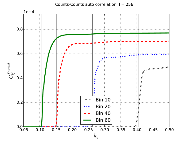
Figure 1: Cumulative contribution to Counts-Counts auto-correlations at $l=256$ from different scales ($C^{\text{Partial}}$). The correlations includes k-values until the limit displayed on the x-axis. Lines in figure corresponds to the redshift bins $0.22<z_{10}<0.23$, $0.34<z_{20}<0.36$, $0.64<z_{40}<0.65$ and $1.00<z_{60}<1.02$

Fig. 1 includes four $C^{\text{Partial}}$ lines for the auto correlations at $l=256$ of galaxy counts in four narrow redshift bins. These auto-correlations include redshift space distortions and a sub-dominant magnification term. From the Limber approximation, one expects the largest contribution from $k=(l+1/2)/\chi(z_{m})$, where $\chi(z_{m})$ is the mean comoving distance of the redshift bin. For the fiducial cosmology one expect the main contribution to the correlations around $k=0.40,0.26,0.15,0.11$ Mpc $h^{-1}$ for the redshift bins $z=0.23,0.35,0.65,1.01$ as shown by the vertical lines in Fig. 1. The estimated scale for the main contribution to the correlation agrees well with the figure.

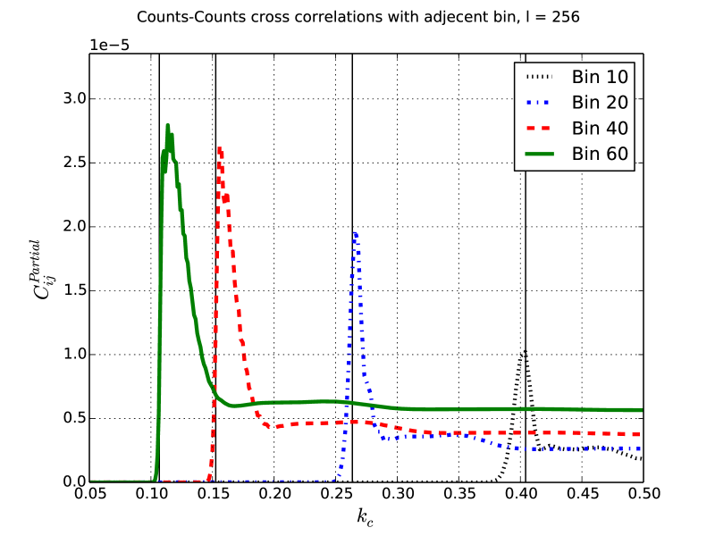
Figure 2: Cumulative contribution to Counts-Counts cross-correlations at $l=256$ from different scales ($C^{\text{Partial}}$). The correlations includes k-values until the limit displayed on the x-axis. The first correlation is between $0.22<z_{10}<0.23$ and $0.23<z_{11}<0.24$, the second between $0.34<z_{20}<0.36$ and $0.36<z_{21}<0.37$, the third between $0.64<z_{40}<0.65$ and $0.65<z_{41}<0.67$, and the fourth between $1.00<z_{60}<1.02$, and $1.02<z_{61}<1.04$.

In figure 2 four thin redshift bins are cross-correlated with the adjacent redshift bin. Each cross-correlation in the figure corresponds to one auto correlation in Fig. 1. Comparing the two figures, similar scales contribute to both the auto and cross-correlations. A characteristic feature of the cross-correlation is the sharp peak. An auto-correlation has only positive contribution as a function of scale, while for a cross-correlation the spherical Bessel functions are slightly out of phase. This results in $k$ values with negative contributions and result in a filtering of small scales (see 4.2.2).

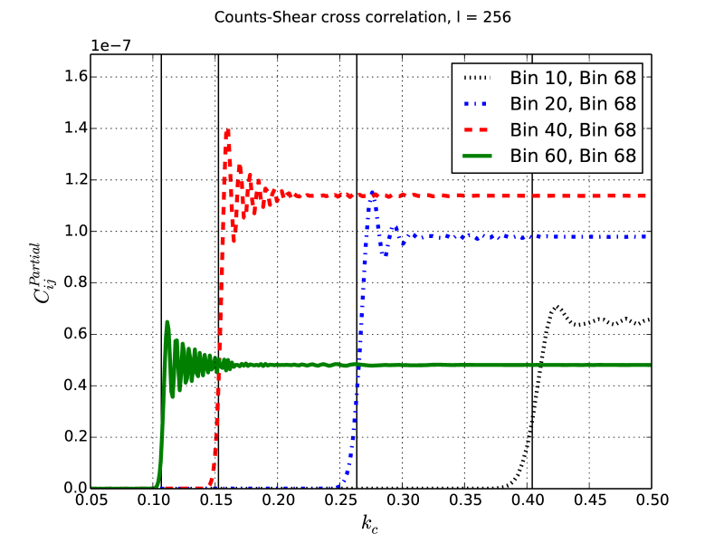
Figure 3: Cumulative contribution to Counts-Shear cross-correlations at $l=256$ from different scales ($C^{\text{Partial}}$). The correlations includes k-values until the limit displayed on the x-axis. For all the correlations the background is $1.16<z_{68}<1.19$, while the foreground redshift bins are $0.22<z_{10}<0.23$, $0.34<z_{20}<0.36$, $0.64<z_{40}<0.65$ and $1.00<z_{60}<1.02$

Fig. 3 cross-correlate overdensities of foreground galaxies with background shear. All lines use the source redshift bin $1.16<z<1.19$, while the foreground redshift bins equals the foreground bins in the previous two figures (Fig. 1 and 2). The scales contributing to the counts-shear cross correlation is precisely the ones contributing to the auto correlation. That is expected from looking at the Limber equations for counts-counts Eq. 14 and counts-shear Eq. 16, both including the power spectrum evaluated at $k=(l+0.5)/\chi(z_{m})$. Further, in the auto-correlation the amplitude increases with redshift because galaxy bias increase with redshift. For counts-shear the correlation peaks with redshift and is lower for the highest redshift bin. This effect comes from the lensing efficiency (Eq. 15), which has a similar peak in redshift. One can also see oscillations around the peak in $k$. These oscillations comes from the galaxy counts being negatively correlated with a redshift range of nearby matter which again lenses the background shear.

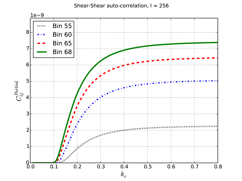
Figure 4: Cumulative contribution to Shear-Shear auto-correlations at $l=256$ from different scales ($C^{\text{Partial}}$). The correlations includes k-values until the limit displayed on the x-axis. Lines correspond to the following thin redshift bins: $0.90<z_{55}<0.92$, $1.00<z_{60}<1.02$, $1.10<z_{65}<1.12$, $1.16<z_{68}<1.19$

Fig. 4 is the shear-shear auto-correlation for four redshift bins. These redshift bins differ from previous figures (Fig. 1 and 2) since the lensing signal is stronger for higher redshift. The signal results from a range of scales because the lensing kernel is broad and the shear-shear correlations convolve two lensing kernels. This is in contrast to the counts-counts and counts-shear which peaks around a specific scale. Even if the lensing kernel is broad, correlating with a narrow foreground redshift bin results in a contribution from a narrow range of scales. Therefore one often describe the shear-shear as a 2D signal, while counts-counts and counts-shear being 3D.

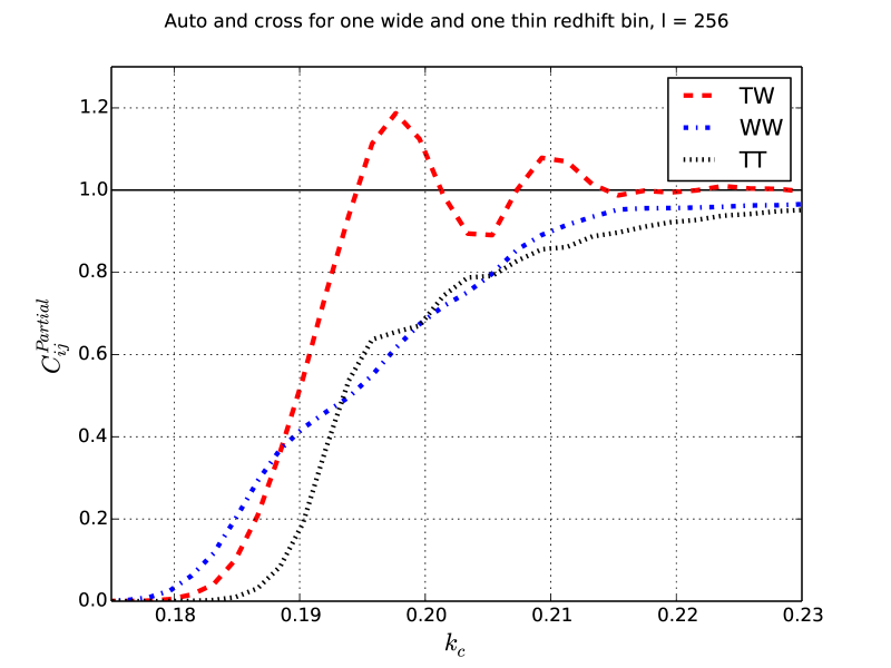
Figure 5: Cumulative contribution for different scales. Auto correlations and the cross correlations for two overlapping thin and thick redshift bins. The thin redshift bin (label T) $0.497<z<0.512$ and the thick one (label W) $0.44<z<0.54$. These bins are selected to include $z=0.5$ and the thick bin is 6.7x wider than the thin redshift bin. To show all three lines together, they are normalized to 1 at the asymptotic value and the scale range is limited.

Fig. 5 includes the count-count auto-correlation for a thin and a thick overlapping redshift bin, together with their cross-correlation. As expected, the thick redshift bin has contributions from a wider range of scales. For a decreasing redshift bin width the correlations does not approach a delta function in scale. Further, as seen in the decline of $C^{\text{Partial}}$, cross-correlations of overlapping redshift bins has both positive and negative contributions. One can understand the effect by decomposing the cross-correlation in the overlapping and non-overlapping regions in redshift. For the overlapping part the cross-correlation behaves similar to the auto-correlation in figure 1, while the non-overlapping parts are like the cross-correlations between adjacent bins in figure 2. The cross-correlation of overlapping bins combines these contributions, but is closer to the auto-correlation which has the strongest signal.

3.8 Converting Cls to $w(\theta)$

So far, this paper has expressed the correlations in Fourier space. Equivalently they could be defined and calculated in $w(\theta)$, which is the 2D correlation function in configuration space. Converting from Cls to $w(\theta)$ is a linear combination (Dodelson, 2003)

$$w(\theta)=\sum_{l}\frac{2l+1}{4\pi}C(l)L_{l}(\cos{\theta})$$ (54)

where $L_{l}$ is the Legendre polynomial of order $l$. The sum is theoretically infinite, while in practice one sum until the result converges. In this subsection we explicitly show how to convert from Cls to $w(\theta)$ using matrix multiplication, to convert multiple correlations in one multiplication. This is afterwards extended to also efficiently integrate of the angular bins in one multiplication.

Let $C_{xl}$ be the 2D correlations in Fourier space stored with the first (x) and second (l) index respectively being the observable and the l-value. Converting from Cl to $w(\theta)$ is done through the matrix multiplication

$$w_{xi}=\sum_{l}C_{xl}S_{li}$$ (55)

where $S$ is defined by

$$S_{li}\equiv\frac{2l+1}{4\pi}L_{l}(\cos{\theta_{i}}).$$ (56)

and $\theta_{i}$ denote the mean of angular bin $i$. The angular bins has a thickness, therefore the correct solution is

$$w[\theta_{A},\theta_{B}]=\frac{1}{\theta_{B}-\theta_{A}}\int_{\theta_{A}}^{\theta_{B}}d\theta w(\theta)$$ (57)

when considering $w(\theta)$ in an angular bin $[\theta_{A},\theta_{B}]$. When using a linear binning in angle, this effect can often be neglected, but results in problems at large angles if using logarithmic spacing in angle and too few bins. The formulas for the integration below uses the Clenshaw-Curtis algorithm.

To integrating over angular bins we first define

$$k_{m} \equiv\cos{\left(\frac{m\pi}{\text{N}_{\text{wbin}}}\right)}$$ (58)

$$x^{\pm}[\theta_{A},\theta_{B}]_{n} \equiv\theta_{B}+\frac{1}{2}(\pm k_{m}-1)(\theta_{B}-\theta_{A})$$ (59)

where $\text{N}_{\text{wbin}}$ is the number of integration points inside each angle bin. The expressions $x^{\pm}$ are the integral points for the two contributions to the integration over an angular bin $[\theta_{A},\theta_{B}]$. If $A$ and $B$ denote the edges of the angular bins and $n$ the number of angular bins, then

$$\theta^{\text{Int}}\equiv\left(x^{-}[\theta_{0},\theta_{1}]\mid x^{+}[\theta_{0},\theta_{1}]\mid\dots\mid x^{-}[\theta_{\text{n}},\theta_{\text{n}+1}]\mid x^{+}[\theta_{\text{n}},\theta_{\text{n}+1}]\right)\\$$ (60)

gives a vector with all intermediate angles in the integration for all angular bins. The integration weights is combined in

$$\phi^{\text{Int}}\equiv\left(\begin{array}[]{ccccccc}w&w&&&&&\\ &&w&w&&&\\ \dots&&\dots&&\dots&&\dots\\ &&&&&w&w\end{array}\right)$$ (61)

where the non-included entries are zero and the matrix is block diagonal. Converting from Cl to $w(\theta)$, also integrating over angle, is done using

$$S^{\prime} \equiv S(\phi^{\text{Int}})^{T}$$ (62)

$$w =C_{l}^{T}S^{\prime}$$ (63)

One could instead use a simpler algorithm leading to less complicated formulas. A key to implementing these formulas is using a mathematical library or language with user friendly array calculations. For example with Numpy (Python library), Eq. 61 can be reduced to a one-line expression. Constructing $s^{\prime}$ is compared to calculating the correlations very fast. In addition these formulas requires estimating $S^{\prime}$ only once for one specific angular bin and maximum summation value in l. When estimating a Fisher matrix or running a MCMC chain, these matrices only needs to be computed once.

4 Impact of Limber, RSD and BAO

First we quantify the importance of using the exact integrals instead of the Limber approximation. Then we study in detail the effects of RSD and BAO on the auto correlations and cross-correlations. In particular because the importance of these effects depends strongly on the redshift bin width. Since a 2D analysis is most widely applied to photometric surveys in broad redshift bins (i.e. $\Delta z\approx 0.1$), it is important to investigate here the effect for the narrower redshift bins ($\Delta z=0.01$) that we are proposing to constrain cosmological models including the effects of BAO and RSD in paper-II. Galaxies are bias through the relation $b(z)=2+2(z-0.5)$, except for the fixed bin in Fig. 23.

The first and second subsection focuses respectively on the auto and cross-correlations. For many of the figures, the same correlations are presented both in Fourier space (Cl) and configuration space $w(\theta)$. Cl plots are directly related to the formalism presented in section 2, but the effect of e.g. BAO are easier to understand using $w(\theta)$. For forecasts the Cls are preferred, since the Gaussian, unmasked and full-sky covariance is block diagonal in l-values. For analyzing data one might prefer $w(\theta)$, since Fourier space correlations can be harder to interpret. Therefore, we include $w(\theta)$ plots to make this section more general than only supporting the forecast.

Signal-to-noise and error bars is an essential part of observational physics. Decades of preparation and billions of dollars are spent, taking a narrow perspective, to reduce the error bars on the measured correlations to improve constraints on cosmological parameters. Effects entering in the correlations are mostly interesting when being comparable large to the error bars. A naively promising signal, might be uninteresting due to low signal-to-noise. The last subsection study the signal-to-noise and the errors on the correlations.

A special case is cross-correlations between partially overlapping bins, which has traits of both auto and cross correlations. These and the non-linear effects are studied in appendix A.

4.1 Auto correlations

4.1.1 Comparing effects as a function of bin width.

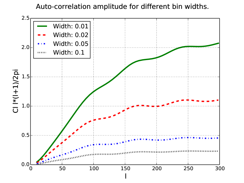
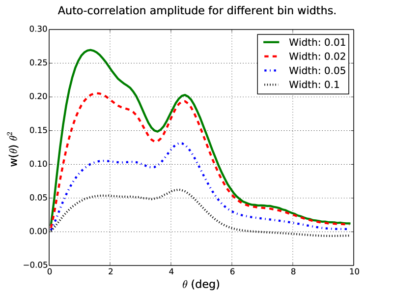
Figure 6: The amplitude of auto-correlations for different redshift bin widths. In both panels the redshift bin centred in $z=0.5$, with the four lines corresponding to redshift bin widths $\Delta z=0.01,0.02,0.05,0.1$. The top and bottom panels correspond respectively to Cl and $w(\theta)$, with the y-label indicating prefactors.

Fig. 6 show the Cl and $w(\theta)$ auto-correlations for different bin width $\Delta z$ . We can see how the amplitude of the overall correlations and the contrast of the BAO wiggles in $C_{l}$ or BAO peak in $w(\theta)$ decrease as we increase $\Delta z$.

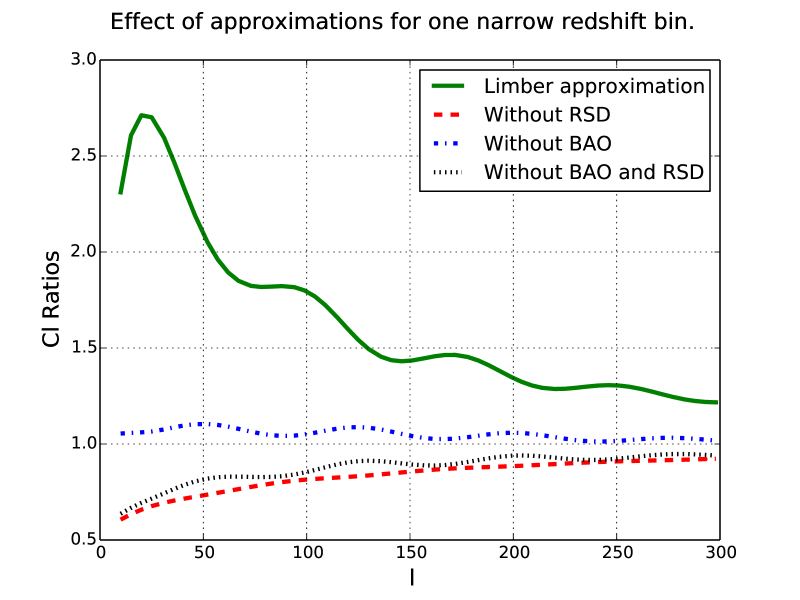
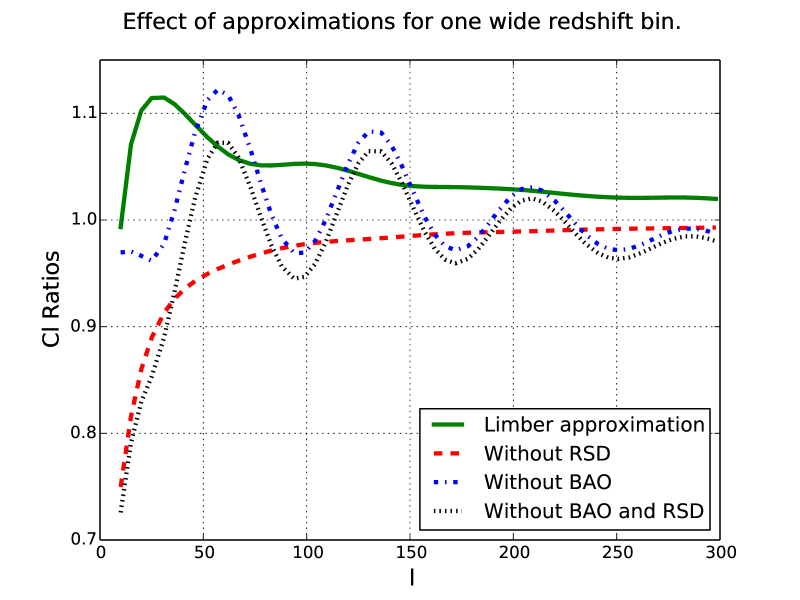
Figure 7: Comparison of the effect of Limber approximations, redshift space distortions and BAO The redshift bin is centred around $z=0.5$ and width $\Delta z=0.01$ (top) or $\Delta z=0.1$ (bottom). Ratios plotted with respect to the exact fiducial calculation (including RSD and BAO), except for the Limber case. Since the Limber approximation is in real space, the ratio is with respect to the real space correlations (i.e. without RSD).

The continues line in Fig. 7 shows the ratio of the Limber approximation to the exact calculation (both without RSD) for $C_{l}$, with the top and bottom panel respectively using a narrow ($\Delta z=0.01$) and wide ($\Delta z=0.1$) redshift bin. All the correlations are centred around $z=0.5$. The other lines show the ratio after removing RSD (dashed), BAO (dot-dashed) or both (dotted). For RSD the ratio is below one, meaning the redshift space distortions contribute positively to the correlations. Including the correlations for two bin widths in Fig.7, show how the relative size of different effects depend on the redshift bin width.

When comparing the effects in a wide and narrow redshift bin, the largest effect comes from the inaccuracy of the Limber approximation in narrow bins. The Limber approximation is known to break down for thin bins. This can be seen in Eq. 14, where the division on the redshift bin width would result in infinite correlations for infinitely thin bins. At $l=150$ the Limber approximations account for $3\%$ for bin width 0.01, which can be tolerated depending on the survey accuracy, while for a narrow redshift bin the effect is close to $50\%$. Which for all purposes is too large.

4.1.2 Limber approximation

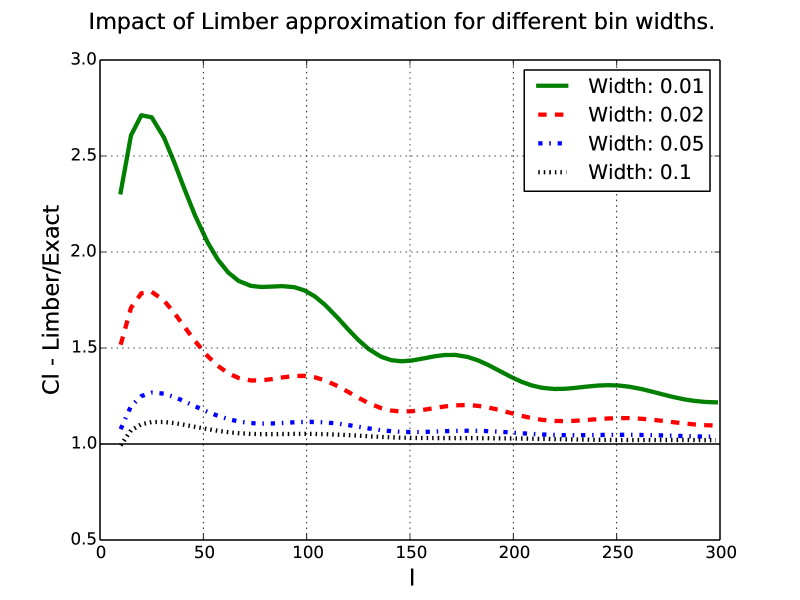
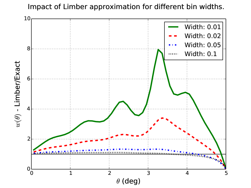
Figure 8: The lines corresponds to bin width 0.01, 0.02, 0.05 and 0.1, centred in $z=0.5$. Both the exact calculations and the Limber approximation is in real space.

The Fig. 8 includes in real space the ratio of the Limber approximation to the exact calculations for both the Cls and $w(\theta)$. From the ratios of the correlations in Fourier space, there is a huge difference is using a wide or a narrow redshift bin. A goal of the forecast in paper-II is to include radial information in the spectroscopic sample. Next subsection show how cross-correlation between adjacent redshift bins which can be used for measuring radial correlation and this requires bins $\Delta z=0.01(1+z)$ for our choice of kmax. From Fig. 8, for our purpose the Limber approximations is unusable even for the auto-correlations.

4.1.3 Redshift space distortions

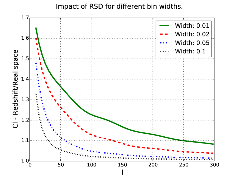
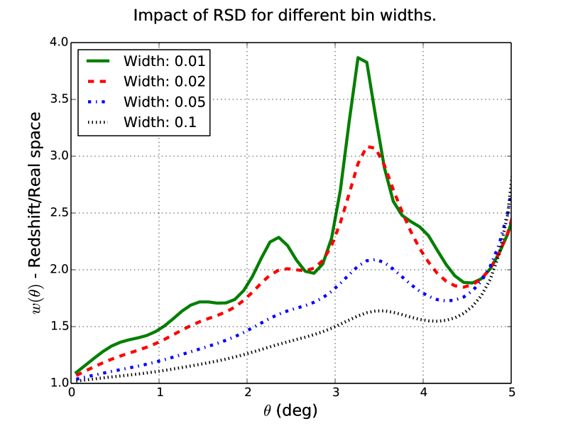
Figure 9: Redshift/real-space ratio in Fourier (top) and configuration space (bottom). The lines corresponds to redshift bin width $\Delta z=0.01,0.01,0.02,0.05,0.1$, centred around $z=0.5$. In this figure ratios about unity means RSD increase the amplitude.

Redshift space distortions (RSD) do not change the angular positions of galaxies, but they do change their angular correlation when selected in observed redshift bins as large-scale motions move structures across the boundaries in a spatially coherent way (see section 2 and references therein). Fig. 9 study the redshift to real-space ratio when varying the redshift bin width. When analyzing galaxy clustering in photometric surveys, the standard approach use 2D-correlations in thick redshift bins. A broad band photo-z scatter RMS is around $0.01(1+z)$ to $0.05(1+z)$ depending e.g. on the magnitude, filters, exposure times and calibration sample. Because of the photo-z scatter, analyzing the data in narrower bins would give little improvements. With narrow bins one would need to model photo-z transitions between redshift bins and their uncertainty (Gaztañaga et al., 2012). For a spectroscopic survey one can analyze the data in narrow bins.

The effect of RSD result in a significant amplitude increase as shown in Fig. 9. A lower bin width results in a higher amplitude. For low values, $10<l<30$, the effect for the broad bin ($\Delta z=0.1$) is $10-30\%$, while the effect is $45-50\%$ for the narrow bin ($\Delta z=0.01$). More importantly, the scales affected depend on the bin width. For the thick redshift (top panel), redshift space distortions only contribute significantly for $l<50$, while for $\Delta z=0.01$ the effect is still  10% at $l=300$. Physically, the redshift space distortions in the 2D-correlations is a boundary effect. When decreasing the bin width, the bulk decrease and the RSD boundary effect becomes more important. This is why Fig.9 looks similar to Fig.8, as the Limber approximation also can be cast as a boundary effect in real space.

In configuration space (Fig. 9, bottom panel), the redshift to real space ratio peaks around 3.5 degrees, shifting only slightly depending on the bin width. For the thinnest bin ($\Delta z=0.01$), the RSD/real space ratio nearly doubles compared to 3 degrees. Increasing the bin width cause the peak to flatten. The higher contribution around 3.5 degrees is caused by BAO in redshift space. From Eq.2.1, the RSD contribution in Fourier space consist of three contributions proportional to spherical Bessel functions of different orders. A small l-value shift give an angular shift in $w(\theta)$. This result in a BAO contribution in $w(\theta)$ which is shifted in angle. We label this contribution the Ghost BAO peak and study its cosmology dependence in subsection 4.1.5.

4.1.4 Baryon acoustic oscillations (BAO)

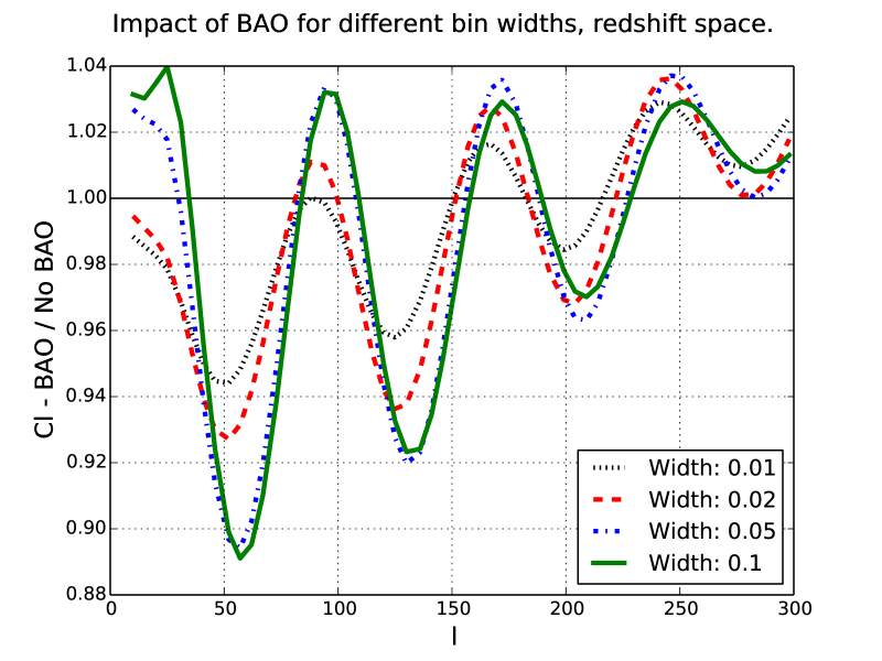
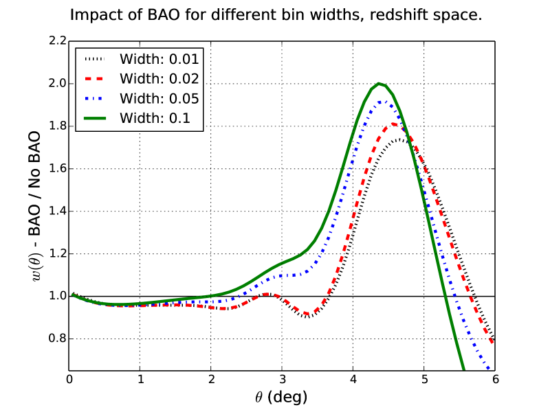
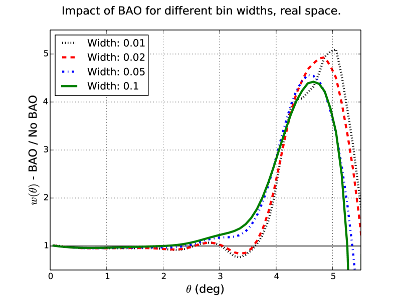
Figure 10: The ratio of correlations including BAO wiggles to a model removing the BAO peak in the EH power spectrum. The first two panels show the ratios in redshift space for Cl and $w(\theta)$. To discuss the effect of redshift space distortions on the BAO peak, the third panel shows the angular correlation in real space. All correlations uses a mean redshift of $z=0.5$ and the bin widths $\Delta z=0.01,0.02,0.05,0.1$.

The three panels in Fig. 10 are included to study the impact of BAO. The first panel show the correlations in Fourier space. One can see how including BAO or using a no-wiggles models leads to oscillation in the ratios. The middle panel shows how the $w(\theta)$ correlation peak around 4.5 degrees for $z=0.5$, shifting towards lower angles for higher redshifts. One see the effect of BAO in redshift space increases when using wider redshift bin. This is counterintuitive, since integrating over the redshift bin results in a convolution in angle. This effect can be understood from redshift space distortions. The bottom panel displays the same ratios in real space, where thicker redshift bins leads to a slight decrease in the BAO signal and a shift in the angle due to projection scales. Including redshift space distortions increases the correlation amplitude, but lower the BAO ratio. The last effect enters since the RSD effect is stronger at lower angles than where BAO peak. For thin bins contribution of redshift space distortions has a narrower peak, which explains why thick bins see a higher contribution on BAO in redshift space.

4.1.5 The Ghost BAO peak

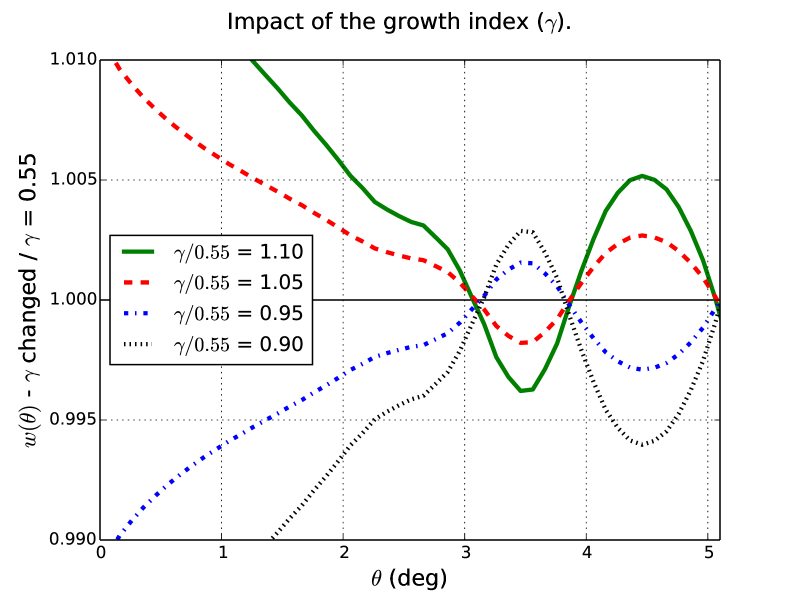
Figure 11: The $w(\theta)$ auto-correlation ratio between a changed growth rate parameter and GR cosmology ($\gamma=0.55$). The auto-correlation use a thin bin ($\Delta z=0.01$), centred in $z=0.5$. Values of $\gamma$ in the ratios are $\pm 5\%,\pm 10\%$ of the fiducial value (see legend).

Fig. 11 illustrates the cosmological dependence of the Ghost BAO peak. As shown in Fig. 9, the RSD contribution peaks at different angular values when measured in narrow redshift bins. In previous figures we assumed the growth rate $\gamma=0.55$ of general relativity. Modified gravity models can change the growth rate (Bueno Belloso, García-Bellido & Sapone, 2011). Increasing $\gamma$ leads to a higher amplitude of the clustering, while lowering the effect of redshift space distortions. This follows from $\frac{\partial D}{\partial f}<0$ and $f\equiv\Omega_{m}(z)^{\gamma}$. In Fig. 11, for higher $\gamma$ the correlations increase for all angles, except around 3.5 degrees where the RSD contribution peaks. While being interesting, note that the amplitude difference is low and the effect might be difficulty to measure.

4.2 Cross correlations between redshift bins

The auto-correlations are the correlation of an observable with itself. Examples are the shear-shear or counts-counts correlation of overdensities in the same redshift bin. A cross-correlation can either come from correlating different quantities as galaxy populations or using different redshift bins for the same quantity. Correlating foreground galaxies with the background shear (Hu & Jain, 2004) or correlating two populations of galaxies (McDonald & Seljak, 2009; Asorey, Crocce & Gaztanaga, 2013) are examples of cross-correlations. In the previous subsection we studied the auto-correlation of galaxy counts in narrow redshift bins. This subsection focus on the 2D cross-correlations between galaxy counts in nearby redshift bins.

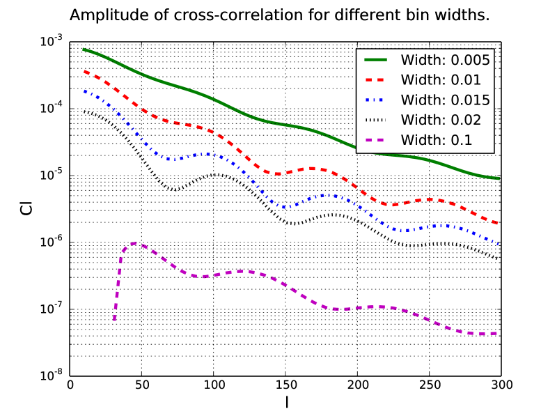
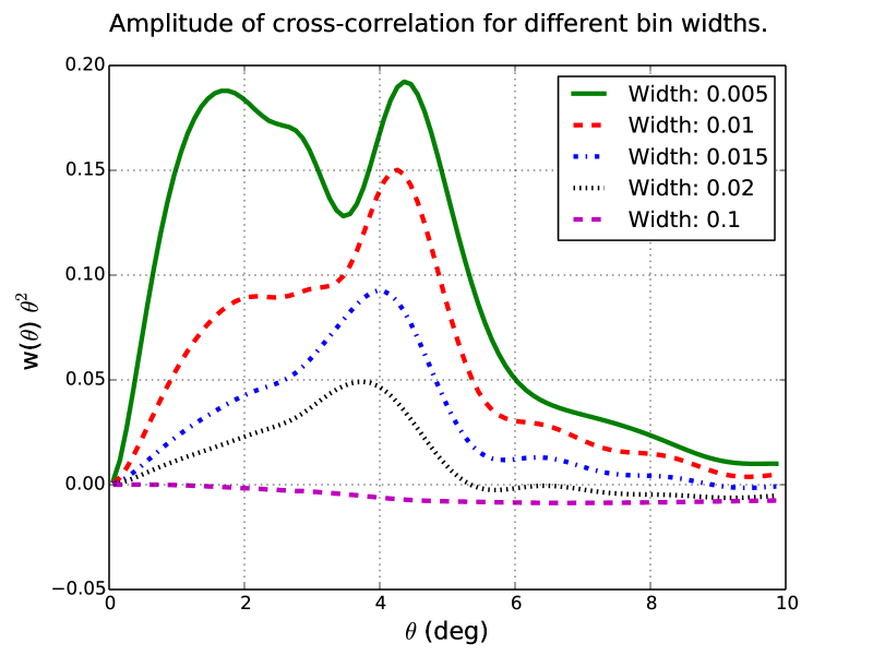
Figure 12: Amplitude of cross-correlations between adjacent redshift bins with equal redshift width. The first redshift bin starts at $z=0.5$ and the five lines correspond to biw width $\Delta z/(1+z)=0.005,0.01,0.015,0.02,0.1$. The top and bottom panels respectively respectively show the Cls and $w(\theta)$ correlations. Here $\Delta z=0.01$ corresponds to the default forecast binning of a spectroscopic sample, while $\Delta z/(1+z)=0.005$ is included to motivate the potential gain by using even thinner redshift bins.

4.2.1 Amplitude of correlations and comparing effects

The intrinsic correlations between two redshift bins is weaker than the auto-correlations and depends strongly on the separation between the redshift bins. Note that the redshift bin cross-correlation presented here are due to correlation of the matter distribution and not from bins overlapping in photo-z space. This distinction is important if studying photo-z surveys in wide redshift bins. The observed cross-correlations $\tilde{C}_{ij}$ including photo-z effects are approximately (Gaztañaga et al., 2012)

$$\tilde{C}_{ij}\simeq r_{ij}C_{jj}+r_{ji}C_{ii}+r_{ii}r_{jj}C_{ij}$$ (64)

where $r_{ij}$ is the fraction of galaxies actually in bin $j$, but observed in bin $i$ due to photo-z inaccuracies. If the two first terms dominate, then the cross-correlations are dominated by the tail of the redshift distribution and not the intrinsic cross-correlation.

Fig. 12 shows the cross-correlations where the first bin starts at $z=0.5$ and the adjacent of two bins. When increasing the bin width from $0.005$ to $0.02$, which is a factor of 4, the amplitude change with an order of magnitude in Fourier space. The rapid decline with increasing bin widths is also seen in the angular correlations. In addition one see a trend where the small scales are affected more than the BAO scale. The amplitude double at 2 degrees using a width of 0.005 instead of 0.01, while the change is 30% at the BAO peak.

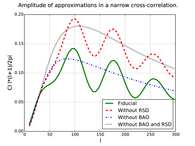
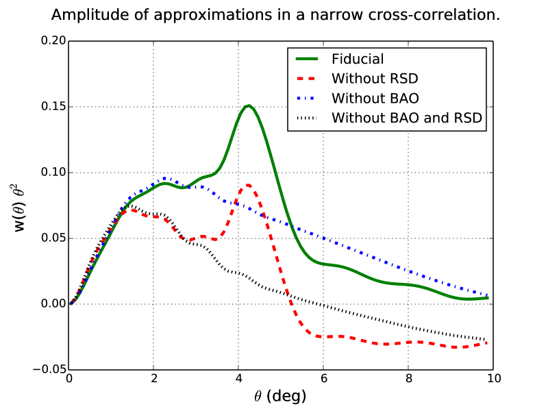
Figure 13: Cross-correlations between adjacent redshift bins. Both bins are $\Delta z=0.01(1+z)$ wide and the first bin starts at $z=0.5$. The four lines include different effects, with the fiducial line including both RSD and BAO. The top and bottom panel respectively show Cls and $w(\theta)$.

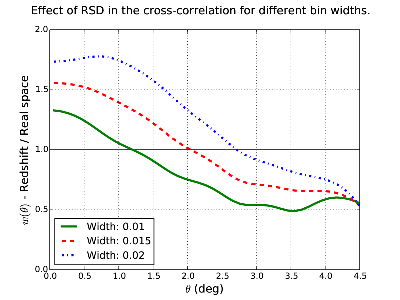
Figure 14: Redshift/real space ratios for the cross-correlation of galaxy counts between adjacent bins. The first bin starts at $z=0.5$ and the three lines corresponds to $\Delta z/(1+z)=0.01,0.015,0.02$. Ratios below unity mean the redshift space distortions suppress the cross-correlations.

Fig. 13 demonstrates how the cross-correlations are affected by BAO, RSD and both effect together. These effects are also strong in the cross-correlations. In the auto-correlations the effect of redshift space distortions increased when decreasing the redshift bin width. Fig. 14 show the effect of RSD for 3 different bin widths. The effect of RSD depend strongly on the separation. Also, for thinner bins the RSD suppresses the signal down to smaller angles.

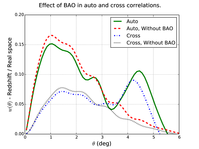
Figure 15: Effect of BAO in the auto and cross correlations. The auto correlations starts at $z=0.5$ with $\Delta z=0.01(1+z)$. In the cross-correlation the second bin is the adjacent bins, which also use $\Delta z=0.01(1+z)$. Both the auto and cross-correlations are shown with and without BAO.

4.2.2 Baryon Acoustic Oscillations.

A characteristic effect in the cross-correlations is an enhancement of BAO. While the effect is present in Fourier space, the physical explanation is simpler in configuration space. Fig. 15 show together an auto- and cross-correlation with and without BAO. Around 1 degree the auto and cross correlations differs by a factor of 2, while they are comparable around the BAO peak. A geometrical interpretation follows from the galaxy pair separation. The galaxy pair separation $r$ can be decomposed into

$$r^{2}=r_{\parallel}^{2}+r_{\perp}^{2}$$ (65)

where $r_{\parallel}$ and $r_{\perp}$ are the distance parallel and perpendicular to the line of sight. The $r_{\perp}$ is measured in an angular separation $\theta$ (on the sky) and converted to a distance through $r_{\perp}\approx\chi(z)\theta$, with $\chi(z)$ being the comoving distance to the closest galaxy. Looking at one fixed angle for the BAO scale corresponds roughly to selecting galaxy pairs with one transverse separation. Galaxy pairs within a thin redshift bins are mostly radially separated around the BAO scale, therefore measuring the angular diameter distances. The cross-correlations between close redshift bins is dominated by the radial BAO, therefore measuring the comoving distance (Gaztañaga, Cabré & Hui, 2009).

The auto and cross-correlations differ radically in the $r_{\parallel}$ distribution of galaxy pairs. For the auto-correlation in $\Delta R$ wide top-hat bins, the probability is highest for zero radial separation and decreases linear towards zero at the bin edges. In the cross-correlation of adjacent bins, the highest probability corresponds to $r_{||}=\Delta R$ and decreases linearly towards the lowest and highest separations. For cross-correlations the redshift bin separation act as a filter around a characteristic distance. In Fig.15, the result can be seen from the small scales being suppressed, while the change is less around the BAO scale.

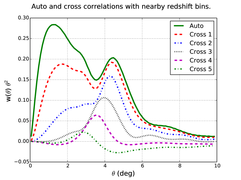
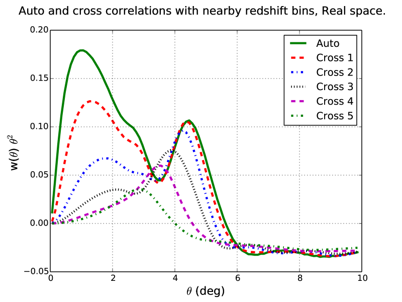
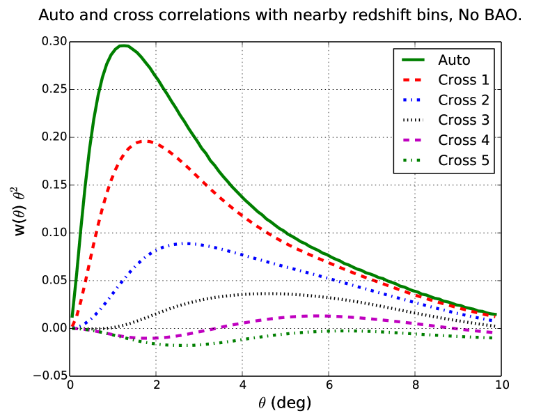
Figure 16: The auto and cross-correlations between close redshift bins. The first redshift bin always starts at $z=0.5$ and all the redshift bin widths are $\Delta z=0.005(1+z)$. We show the auto correlation (auto) and correlation with the adjacent bin (cross 1) and the four next closest redshift bins at higher redshift. In the legend ”corr n” means the redshift bin index of the two observable differs with n, i.e. 1 is the adjacent bin. The top, middle and bottom panels show respectively the fiducial, real space and no-wiggle correlations.

The cross-correlations filter away small scales also when the bins are separated, although the distribution of radial distances ($r_{\parallel}$) changes. Fig.16 include the cross-correlations between more bins. For larger redshift bin separation the suppression of small scales in the cross-correlations become stronger. On the other hand, for the BAO scale the first cross-correlations are comparable to the auto-correlation. Here the gap between two redshift bins introduce a lower limit on the galaxy pair separation. As the separation between the bins increase, the distance filtered out gradually grows above the BAO scale of 150 Mpc. For larger separation, as seen in the last cross-correlations, the peak is also affected.

For angles above 3.5 deg., the last cross-correlation in Fig. 16 becomes negative. Unlike the auto-correlation which is positive (for the relevant angles), the cross-correlation can also be negative. In Fourier space (Cls), the negative cross-correlations can be understood from the spherical Bessel function in Eq.2 and 3. For an infinitesimal thin redshift bin the fluctuations $\delta_{l}(z,k)$ are proportional to $j_{l}(kr(z))$, where $r(z)$ is the comoving distance to the redshift bin. When cross-correlating two redshifts the oscillations might be out of phase, which generates a negative contribution. The integral over the redshift bins is (in real space) a linear superpositition of two such Bessel functions. For thick bins negative contributions average out and thin redshift bins increase the probability of finding negative correlations.

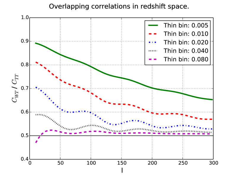
Figure 17: Ratio $C_{WT}/C_{TT}$ where W and T are a wide and thin bin. Both bins are centred around $z=0.5$, with $\Delta Z_{Thick}=2\Delta Z_{Thin}$. The lines corresponds to using $\Delta z/(1+z)=0.005,0.01,0.02,0.04,0.08$ for the thinnest redshift bin.

4.2.3 Partial overlapping bins

The correlations discussed so far has either been auto-correlations or cross-correlations of non-overlapping redshift bins. One can for galaxy counts use a multi-tracer strategy and split the galaxy sample into different populations. For example including two galaxy populations with very different bias reduce the sample variance. In the forecast we use the spectroscopic and photometric surveys as two different populations. The spectroscopic binning is 7 times thinner (than the photometric sample) to capture the radial information. When cross-correlating overlapping photometric and spectroscopic surveys, it naturally leads to cross-correlations of redshift bins with different width.

Fig. 17 show the cross-correlation of galaxy counts in two overlapping redshift bins with $\Delta Z_{Wide}=2\Delta Z_{Thin}$. The ratio shown is $C_{WT}/C_{TT}$, where T and W respectively denotes wide and thin bins. In the Limber approximation, the auto-correlation is inverse proportional to the bin width. If all the correlation of the overlapping cross-correlation is due to galaxy pairs in the overlapping region, one expect $C_{WT}/C_{TT}=0.5$ for the Limber approximation in real space. For the relatively thick bins of $\Delta z=0.04,0.05$, the ratio is close to the Limber ratio (0.5). Cross-correlation of thinner bins increases the ratio. For the three thin redshift bins of 0.005, 0.01 and 0.02 the overlapping correlation is higher than what is expected from counting galaxy pairs in the overlapping region. When using two overlapping bins, the galaxies are not only correlating inside the overlapping redshift region, therefore increasing the correlation.

4.3 Errors and signal to noise.

The cosmic variance errors when assuming Gaussian fluctuations are (Dodelson, 2003)

$$Cov(C_{ij},C_{mn}) =N^{-1}(l)\left(C_{im}C_{jn}+C_{in}C_{jm}\right)$$ (66)

$$Var(C_{ij}) =N^{-1}(l)\left(C_{ii}C_{jj}+C_{ij}^{2}\right)$$ (67)

$$Var(C_{ii}) =2N^{-1}(l)C_{ii}^{2}$$ (68)

where $N(l)=2f_{sky}(2l+1)$ is the number of modes and $f_{sky}$ is the sky fraction covered by the survey. The first line give the general covariance expression, while the second and third line respectively give the variance for an auto and cross-correlation. Additionally the counts-counts correlation ($C_{g_{i}g_{j}}$) include a shot-noise from sampling a finite number of galaxies and shape measurement errors affect the shear-shear correlations. Let $\tilde{C}$ and $C$ respectively denote the correlations including or not the measurement errors. The observed correlations are

$$\tilde{C}_{g_{i}g_{j}} =C_{g_{i}g_{j}}+\delta_{ij}\frac{1}{N_{i}}$$ (69)

$$\tilde{C}_{\gamma_{i}\gamma_{j}} =C_{\gamma_{i}\gamma_{j}}+\delta_{ij}\frac{\sigma^{2}_{\gamma}}{N_{i}}$$ (70)

where $N_{i}$ is the observed galaxy number in bin $i$ per stereo-radian and $\sigma_{\gamma}^{2}$ is the average shear measurement variance.

Fiducially to match the forecast, we assume a 0.4 gal/sq.arcmin. dense sample magnitude limited to $i_{AB}<22.5$ and a galaxy bias of $b(z)=2+2(z-0.5)$. The correlation in this subsection use $z=0.5$, which means $b=2$. These values are selected to match the spectroscopic sample in the forecast. Note that the errors shown in Fig.24 are dominated by cosmic variance. The exact $n(z)$ details (see paper-II) is therefore less important. All signal-to-noise (S/N ) plots assume 1000 sq.deg. survey area.

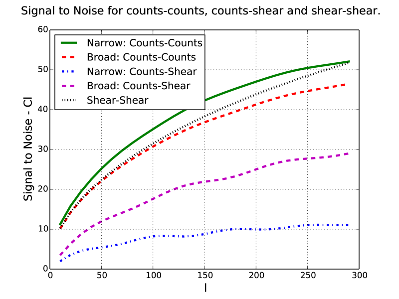
Figure 18: Signal-to-Noise for different types of correlation. Two galaxy populations are included, a foreground population for measuring galaxy counts and a background population for Faint galaxies. In two lines corresponding to Count-Counts and Counts-Shear, a thin bin of $\Delta z=0.001$, $z=0.5$ is used, while the other two uses a thick bin of $\Delta z=0.01$, $z=0.5$. The background bin at $z=1.1$ is $\Delta z=0.15$ wide. Last the figure show the Shear-Shear S/N ratio for the background shear used for both the Counts-Shear correlations.

Fig.18 show the S/N for different counts-counts, counts-shear and shear-shear correlations. An important point of this figure is to compare how the redshift bin width affect the S/N . Therefore the counts-counts and counts-shear correlations are both shown with a thin and a thick foreground bin (see caption). For zero shot-noise, the S/N of the counts-counts auto-correlations are

$$(S/N)[C_{g_{i}g_{i}}]\equiv\sqrt{N(l)/2}$$ (71)

which is independent of the redshift bin width. The two count-counts auto correlation lines differs in shot-noise covering different redshifts since one set of bins are wider. Except this, the signal to noise for the two auto-correlations does not depend on the redshift bin width. The counts-shear S/N is directly dependent on the lens bin width. From the Limber approximation, the counts-counts auto-correlation in the variance is inversely proportional to the bin width ($C_{ii}\propto 1/\Delta_{i}$). On the other hand, the counts-shear signal is independent of the foreground bin width when ignoring the cosmological evolution in the lens bin. Combined these two expressions lead to

$$(S/N)[C_{g_{i}\gamma}]\propto\sqrt{\Delta_{i}}$$ (72)

where $\Delta_{i}$ is the redshift bin width. This means the S/N of a single counts-shear cross-correlation decrease when using a thinner lens redshift bin. In Fig. 18, the two counts-shear S/N lines use $\Delta z=0.01$ and $\Delta z=0.1$ wide lens bins. A cross-correlation with 10 times thinner redshift bins should result in around 3 times lower S/N . While each correlation becomes noisier when decreasing the lens bin width, the reduced width allow for more bins. The number of bins is proportional to $1/\Delta_{i}$. Therefore the combined S/N for all counts-shear correlations scale with $\sqrt{\Delta_{i}}$. In addition thinner lens bins has the advantage of less projection in redshift.

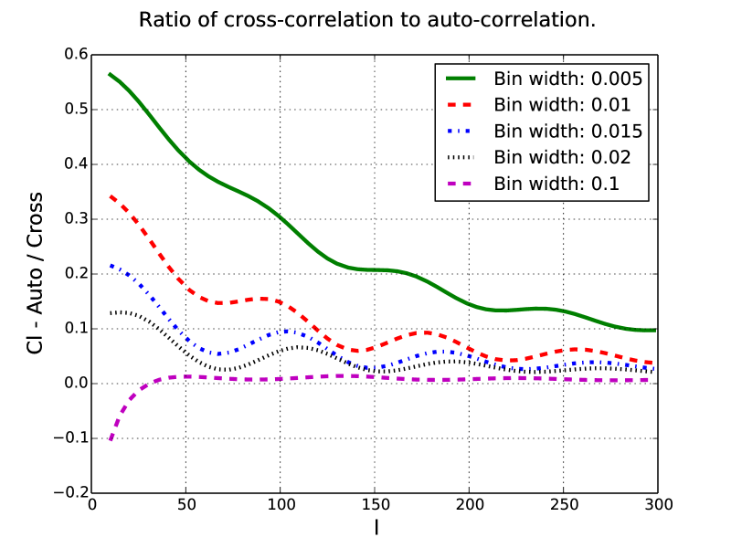
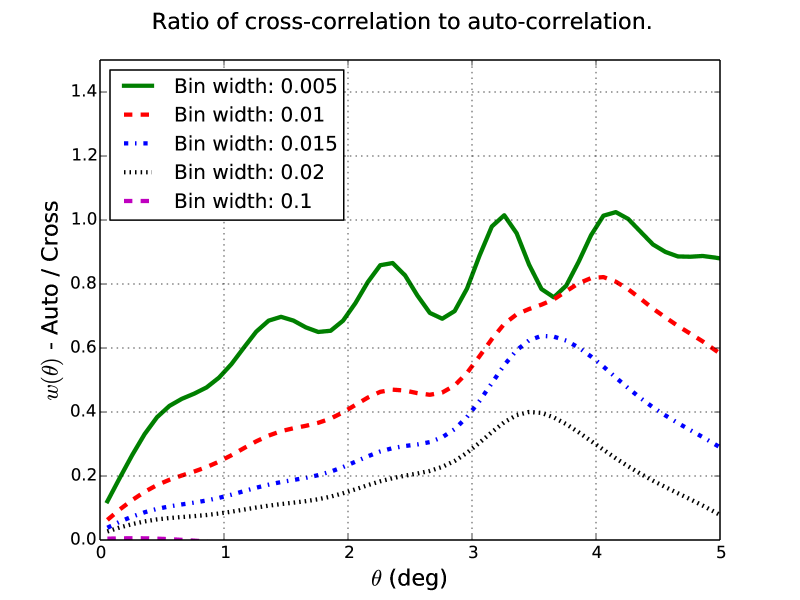
Figure 19: Auto/cross-correlation ratio for galaxy counts. The auto-correlation bin starts at $z=0.5$, with the four lines corresponding to $\Delta z=0.005,0.01,0.015,0.02$. The cross-correlation is between the auto-correlation bin and the adjacent bin at higher redshift. Both redshift bins are equally wide. In the top and bottom panel, the figure respectively show the ratio in Fourier and configuration space.

Subsection 4.2 studied the galaxy counts cross-correlation between adjacent redshift bins. These correlations can, if the S/N is sufficient, measure radial information. The S/N for the cross-correlations between different redshift bins are directly related to the cross/auto correlations ratio. This follow from

$$\frac{(S/N)[C_{ij}]}{(S/N)[C_{ii}]} =\sqrt{2}\frac{C_{ij}}{C_{ii}}\frac{C_{ii}}{\sqrt{C_{ii}C_{jj}+C_{ij}^{2}}}$$ (73)

$$\approx\sqrt{2}\frac{C_{ij}}{C_{ii}}{\left(1+{(\frac{C_{ij}}{C_{ii}})}^{2}\right)}^{-1/2}$$ (74)

$$\approx\sqrt{2}\frac{C_{ij}}{C_{ii}}$$ (75)

where the second and third line respectively use $C_{ii}\approx C_{jj}$ and $C_{ij}<<C_{ii}$. Approximating the auto-correlations ($C_{ii}\approx C_{jj}$) works for equally wide and thin bins. When $C_{ii}/C_{ij}=2.1,6.9$ the last approximation is respectively accurate to 10% and 1%. The S/N ratio can be understood from the cross-correlation variance being dominated by the auto-correlation variance.

Fig.19 top panel show the ratio $C_{ij}/C_{ii}$ for various bin widths. When increasing the bin width, the ratio decline quickly due to $C_{ij}$ being sensitive to the redshift bin separation. If using $\Delta z=0.005$ instead of $\Delta z=0.01$, the $C_{ij}/C_{ii}$ ratio doubles. The bottom panel show the $w_{ij}(\theta)/w_{ii}(\theta)$ ratios. Another interesting aspect is looking at $w(\theta)$ the cross-correlations are having a high signal at large angles. For example the cross-correlation with bin-width of 0.01 is $40\%$ of the auto-correlation at 2 degrees and $80\%$ at 4 degrees. This means the cross-correlations is gaining a higher signal to noise at larger angles.

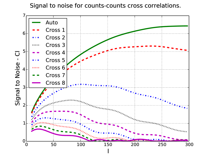
Figure 20: Cross-correlations between very narrow redshift bins. All bins are $\Delta z=0.001(1+z)$ wide and the first redshift bin start at $z=0.5$. The auto-correlation is for the first redshift bin, while ”Cross X” corresponds to a cross-correlation of the first bin with a bin separated by X time $\Delta z$.

To illustrate the effect of cross-correlations, Fig. 20 shows the signal-to-noise for extremely thin redshift bins. These redshift bins are $\Delta z=0.001(1+z)$ wide, which would correspond to 694 redshift bins for $0.1<z<1.2$. From the figure, one see there is a sharp drop in S/N when increasing the distance between the redshift bins. Also, the change is lower at low l-values, which make the cross-correlations more important at large scales. For the forecast in $\Delta z=0.01(1+z)$ wide bins, the main contribution comes from the auto-correlation and cross-correlation with the adjacent bin.

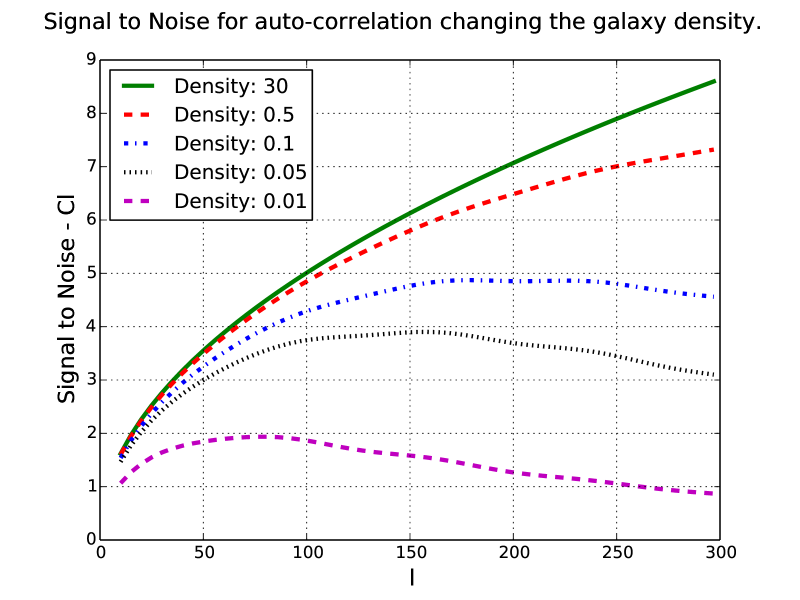
Figure 21: Signal-to-noise for different galaxy densities. The auto-correlation redshift bin is centred in $z=0.5$ and is $\Delta zz=0.01(1+z)$ wide. The S/N is calculated for 0.01, 0.05, 0.1, 0.5 and 30 gal/sq.arcmin in the full sample. In addition 50% is removed to simulate various cuts.

Finally Fig. 21 shows the S/N for auto-correlations in the redshift bin $z=0.5$, $\Delta z=0.01(1+z)$ for different densities. The upper line with 30 gal/sq.arcmin, which is lower than the expected LSST density of 40 gal/sq.arcmin (LSST Science Collaboration et al., 2009), is approximately noiseless for the counts-counts auto-correlation. A line with 0.5 gal/sq.arcmin is close to the spectroscopic density used in the forecast (0.4 gal/sq.arcmin). For the l-values considered for the forecast ($l\leq 300$), the dense spectroscopic sample has a S/N close to the noiseless limit. These conclusions does however vary with lmax and also with the redshift one study.

5 Conclusion

In this paper we have studied the modelling of galaxy clustering, RSD and WL with angular cross-correlations. Lensing is often studied using 2D correlations, while clustering and RSD is analyzed with the 3D power spectrum. Combining WL, large scale structure and RSD is from a theoretical viewpoint significantly easier using the angular correlation functions. Directly constructing observable in angles (or multipoles) and redshifts avoids the model assumptions that are needed in a 3D analysis when converting distances. Moreover, the expression for the covariance is straight forward. Using only angular correlations avoids double counting transverse information and can naturally account for potential redshift uncertainties in the LSS analysis by migration matrices (Gaztañaga et al., 2012).

One practical concern is the efficiency of implementing a computer code for predicting the angular correlation function. Analyzing a spectroscopic sample using 2D-correlations requires a large number of redshift bins to capture the radial information. In section 3 we introduced an algorithm specialised on calculating the cross-correlations between many redshift bins and with multiple tracers. Instead of calculating each correlation separately, all correlations are calculated at once. This allows for reusing parts of the calculations and extensive use of matrix multiplication. In particular, the integration between all correlation of redshift bins is expressed using a matrix products. Being formulated in terms of array operations and matrix multiplications allows for an efficient implementation, even in high level languages (e.g. Python) with bindings to high performance linear algebra implementations.

Section 4 began with studying the effect of BAO, RSD and the Limber approximation for the auto and cross-correlations. For the auto-correlation of $\Delta z=0.1$ thick bins, the Limber approximation can be sufficient for a small area survey. In narrow redshift bins ($\Delta z=0.01$), which is needed for the forecast, the Limber approximation completely breaks down. Redshift space distortions leads to 30% larger amplitude for the galaxy counts auto-correlations in broad bins. For thin bins ($\Delta z=0.01$), the RSD effect can result in 2.5-3 times higher auto-correlations at low multipoles. In addition for thinner bins the effect of redshift space distortions clearly shows a peak in angle. We showed that this second peak, which we named the ghost BAO peak, results from the BAO peak being shifted in redshift space.

The cross-correlation of nearby redshift bins unexpectedly has a larger BAO contribution than the auto-correlations. When cross-correlating two redshift bins, the bin separation affects the radial pair separation. In cross-correlations the most probable radial galaxy separation is the distance between the mean of the two redshift bins. Therefore cross-correlations include pairs with higher radial separation, which suppress small-scale clustering and lead to a larger BAO contribution. Galaxy pairs within a thin redshift bins are mostly radially separated around the BAO scale, therefore measuring the angular diameter distances. The cross-correlations between close redshift bins is dominated by the radial BAO, which measures the comoving distance (Gaztañaga, Cabré & Hui, 2009). We have also shown in section 4.3 that the signal-to-noise (S/N ) is larger in the cross-correlation at BAO scales.

We also studied the S/N for different correlations. The counts-counts correlations has the highest signal-to-noise, while the counts-shear and shear-shear correlation have a lower S/N ratio. In the count-shear correlation the bin width of the galaxy counts in the lens bin directly affects the noise, while the signal is only affected by projection effects. Each correlation of narrow bins has a lower signal-to-noise. However the total S/N is higher since the thinner bins result in more counts-shear cross-correlations. Finally we looked at the sensitivity of galaxy density for the counts-counts auto-correlations. For a dense galaxy sample (0.4 gal/sq.arcmin), used for the spectroscopic sample in the forecast, the S/N for $z=0.5$ is close to the noiseless limit.

Altogether our results show that this new approach to clustering analysis, using angular cross-correlations in narrow redshift bins, is potentially viable: it recovers all the 3D information (Asorey et al., 2012; Asorey, Crocce & Gaztanaga, 2013), it can be predicted with a fast algorithms and it contains new insights of physical effects such as WL, RSD and BAO. In the following papers of this series we will present different applications and results using the formalism presented here.

Appendix A Auto and cross correlations

A.1 Redshift space distortions

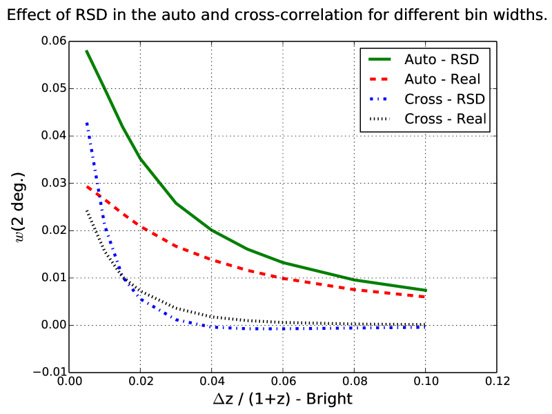
Figure 22: Contribution of RSD for the auto- and cross-correlations with the adjacent bin when varying the redshift bin width. Both redshift bins are equally wide (at $z=0$), with the width given on the x-axis. The correlations are shown at 2 degrees and the first redshift bin starts at $z=0.5$.

The RSD dependence on the redshift bin width is illustrated in Fig.22. An additional redshift from peculiar line-of-sight velocities can move galaxies between redshift bins, which cause the RSD signal. In thin redshift bins more galaxies move between the bins, therefore thin bins increase the RSD signal. For the thinnest bin ($\Delta z=0.005$) the auto-correlation has double the amplitude in redshift compared to real space. When increasing the bin width, both the signal and fraction of RSD signal decrease. For cross-correlations, the redshift space distortions can contribute positive or negatively, depending on the bin width. In this configuration, below $\Delta z\approx 0.015$ the RSD increase the cross-correlation, which suppressing the signal for wider redshift bins. For thick redshift bins ($\Delta z=0.05-0.1$) the cross-correlations is negative in redshift space.

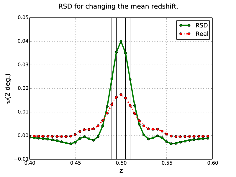
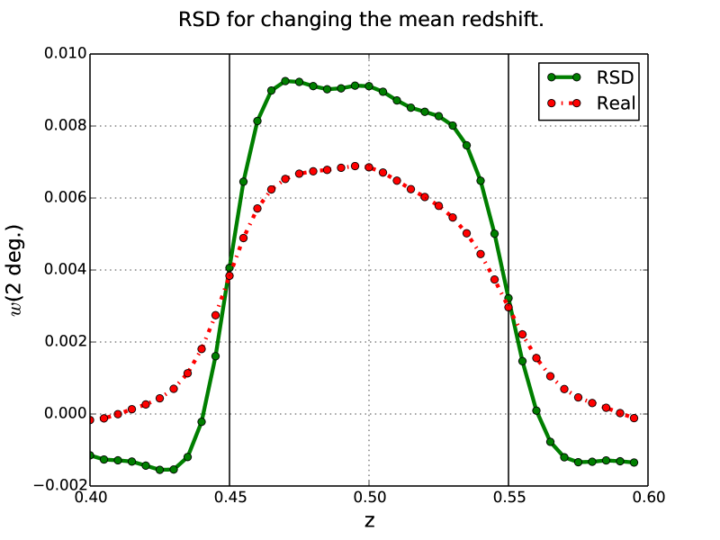
Figure 23: The cross-correlation when changing one bin position. In both panels, one redshift bin is fixed at $z=0.5$ and the second redshift mean vary as indicated on the x-axis. The top panel correlate two thin ($\Delta z=0.01$) redshift bins. The two inner vertical lines ($z=0.495,0.505$) mark the fixed redshift bin, while the two outer lines ($z=0.49,0.51$) mark when the bins have no redshift overlap. In the bottom panel, the fixed bin is thick ($\Delta z=0.1$), while the varying bin is thin ($\Delta z=0.01$). In the fixed bin, the bias $b(z)=1.2+0.4(z-0.5)$ is used. Here the vertical lines ($z=0.45,0.55$) mark the fixed bin. The two lines show the correlation in redshift and real space.

Fig. 23 shows a $w(\theta)$ cross-correlation amplitude when shifting one redshift bin, while the other is centred around $z=0.5$. In the top panel, both redshift bins are $\Delta z=0.01$ wide and the inner vertical lines mark the fixed bin. For two narrow and fully overlapping bins, the signal double in redshift space. When reducing the amount of overlap, both the clustering in real space and redshift space decreases. The two outer vertical lines marks having redshift bins side by side. In this configuration, the correlations are still positive. For larger separation the redshift space distortions suppress the signal, which was also seen in Fig. 22.

In the bottom panel the fixed bin is thick ($\Delta z=0.1$), while the bin changing position is still thin ($\Delta z=0.01$). For fully overlapping bins and close centers the signal is fairly flat. When the thin bin move closer to the edge, but they still overlap, the signal falls off sharply. The decrease in the cross-correlation amplitude comes from removing part of the non-overlapping cross-correlations between the bins. When the bins move apart, the signal clearly becomes negative in redshift space.

A.2 Non-linear effects

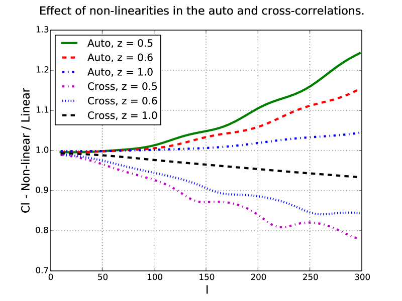
Figure 24: The impact of non-linear effect in the auto and cross-correlations for different redshifts. The figure show non-linear/linear correlation function ratio, with non-linear including Halofit contributions to the linear EH power spectrum. All redshift bins are $\Delta z=0.01(1+z)$ wide, the cross-correlation is with the adjacent bins and the redshifts $z=0.5,0.6,1.0$ give the start of the first redshift bin.

Non-linear gravitational effects enhance the dark matter power spectrum on small scales. The EH and CAMB (Lewis, Challinor & Lasenby, 2000) power spectrum models only the linear power spectrum. For modelling the non-linear effects, one can create fitting formulas based on n-body simulations or use pertubation theory. The Halofit-II power spectrum model is based on a series of simulations to model non-linear gravitational effects (Smith et al., 2003; Takahashi et al., 2012). To include the Halofit only require implementing the model and providing a linear power spectrum, for which we use the Eisenstein-Hu.

Fig. 24 shows the non-linear/linear Cl ratios. The ratios are for auto and adjacent cross-correlations in the redshift bins $z=0.5,0.6,1.0$ and with $\Delta z=0.01$. The non-linear effects in the power spectrum increase with the comoving wavenumber ($k\equiv l/\chi(z)$). As expected, the effect increase with l and lower redshifts has the highest non-linear contributions. The oscillations seen are due to the BAO. In the cross-correlations, the non-linear effects suppress the signal. Previously, we showed (Fig. 2) how counts-counts cross-correlations in narrow bins has both a positive and negative contribution from different scales. Since higher k-values contribute negatively and the non-linear effect increase with scale, this leads to non-linear effects suppressing the cross-correlations.

Appendix B Clenshaw-Curtis integration

B.1 Overview

The Clenshaw-Curtis integration algorithm expands the integrand in Chebyshev polynomials and works well for oscillating integrals. Integrating $f$ over the interval $[-1,1]$ can be approximated

$$\int_{-1}^{1}f(x)dx\approx\sum_{n=0}^{N/2}\mathcal{W}_{n}{f(\cos[n\pi/N])+f(-\cos[n\pi/N])}$$ (76)

where $N$ is the number of integration points. The coefficients $\mathcal{W}_{n}$ are given by

$$d_{i} =\begin{cases}1&i=0\\ \frac{1}{1-N^{2}}&i=N/2-1\\ \frac{1}{1-{(2i)}^{2}}&\text{Otherwise}\end{cases}$$ (77)

$$D_{ij} =\frac{2}{N}\cos{\left(\frac{2ij\pi}{N}\right)}$$ (78)

$$\mathcal{W} =D^{T}d$$ (79)

where the last equation uses matrix multiplication.The integration in Eq.76 can be transformed to different integration limits. For example when integrating over scales, one have

$$\int_{k_{min}}^{k_{max}}f(k)dk=k_{w}\int_{-1}^{1}f(\bar{k}+k_{w}x)dx$$ (80)

where the integration variable is defined by $k=\bar{k}+k_{w}x$, $\bar{k}\equiv\frac{1}{2}(k_{min}+k_{max})$ and $k_{w}\equiv\frac{1}{2}(k_{max}-k_{min})$.

B.2 Change of integral domain for the tomographic integration.

The Cl integrand is on the form $f(x)\equiv G_{i}(x)G_{j}(x)$. When trying to integrate by multiplication, the expansion Eq.76 into two terms creates an additional complication. Expanding the terms, one find

$$\begin{split}\int_{-1}^{1}G_{i}(x)G_{j}(x)dx=&\sum_{n=0}^{N/2}G_{i}(\cos(n\pi/N))G_{j}(\cos(n\pi/N))\\ &+G_{i}(\cos(-n\pi/N))G_{j}\left(-\cos(n\pi/N)\right).\end{split}$$ (81)

Through defining

$$y^{+}_{in} =G_{i}(\cos(n\pi/N))$$ (82)

$$y^{+}_{jn} =G_{i}(-\cos(n\pi/N))$$ (83)

the integration can be written

$$\int_{-1}^{1}G_{i}(x)G_{j}(x)dx=\sum_{n}w_{n}(y^{+}_{in}y^{+}_{jn}+y^{-}_{in}y^{-}_{jn}).$$ (84)

References

- Abdalla et al. (2012) Abdalla F. et al., 2012, ArXiv e-prints
- Amendola et al. (2013) Amendola L. et al., 2013, Living Reviews in Relativity, 16, 6
- Amiaux et al. (2012) Amiaux J. et al., 2012, SPIE Astronomical Telescopes and Instrumentation Proceedings SPIE8442-32, 2012
- Anderson et al. (2014) Anderson L. et al., 2014, MNRAS, 439, 83
- Asorey et al. (2012) Asorey J., Crocce M., Gaztañaga E., Lewis A., 2012, MNRAS, 427, 1891
- Asorey, Crocce & Gaztanaga (2013) Asorey J., Crocce M., Gaztanaga E., 2013
- Bartelmann & Schneider (2001) Bartelmann M., Schneider P., 2001, Phys. Rep., 340, 291
- Bernstein & Cai (2011) Bernstein G. M., Cai Y.-C., 2011, MNRAS, 416, 3009
- Blas, Lesgourgues & Tram (2011a) Blas D., Lesgourgues J., Tram T., 2011a, CLASS: Cosmic Linear Anisotropy Solving System. Astrophysics Source Code Library
- Blas, Lesgourgues & Tram (2011b) Blas D., Lesgourgues J., Tram T., 2011b, J. Cosmology Astropart. Phys, 7, 34
- Bueno Belloso, García-Bellido & Sapone (2011) Bueno Belloso A., García-Bellido J., Sapone D., 2011, J. Cosmology Astropart. Phys, 10, 10
- Cai & Bernstein (2012) Cai Y.-C., Bernstein G., 2012, MNRAS, 422, 1045
- Challinor & Lewis (2011a) Challinor A., Lewis A., 2011a, CAMB Sources: Number Counts, Lensing & Dark-age 21cm Power Spectra The linear power spectrum of observed source number counts. Astrophysics Source Code Library
- Challinor & Lewis (2011b) Challinor A., Lewis A., 2011b, Phys. Rev. D, 84, 043516
- Crocce, Cabré & Gaztañaga (2011) Crocce M., Cabré A., Gaztañaga E., 2011, MNRAS, 414, 329
- Crocce et al. (2010) Crocce M., Fosalba P., Castander F. J., Gaztañaga E., 2010, MNRAS, 403, 1353
- Crocce, Scoccimarro & Bernardeau (2012) Crocce M., Scoccimarro R., Bernardeau F., 2012
- de Putter, Doré & Takada (2013) de Putter R., Doré O., Takada M., 2013, ArXiv e-prints
- Dodelson (2003) Dodelson S., 2003, Modern cosmology
- Eisenstein & Hu (1998) Eisenstein D. J., Hu W., 1998, ApJ, 496, 605
- Fisher et al. (1995) Fisher K. B., Huchra J. P., Strauss M. A., Davis M., Yahil A., Schlegel D., 1995, ApJS, 100, 69
- Fisher, Scharf & Lahav (1994) Fisher K. B., Scharf C. A., Lahav O., 1994, MNRAS, 266, 219
- Font-Ribera et al. (2013) Font-Ribera A., McDonald P., Mostek N., Reid B. A., Seo H.-J., Slosar A., 2013, ArXiv e-prints
- Fosalba et al. (2008) Fosalba P., Gaztañaga E., Castander F. J., Manera M., 2008, MNRAS, 391, 435
- Fu et al. (2008) Fu L. et al., 2008, A&A, 479, 9
- Gaztañaga, Cabré & Hui (2009) Gaztañaga E., Cabré A., Hui L., 2009, MNRAS, 399, 1663
- Gaztañaga et al. (2012) Gaztañaga E., Eriksen M., Crocce M., Castander F. J., Fosalba P., Marti P., Miquel R., Cabré A., 2012, MNRAS, 422, 2904
- Hamilton (1998) Hamilton A. J. S., 1998, in Astrophysics and Space Science Library, Vol. 231, The Evolving Universe, Hamilton D., ed., p. 185
- Heymans et al. (2013) Heymans C. et al., 2013, MNRAS, 432, 2433
- Hu & Jain (2004) Hu W., Jain B., 2004, Phys. Rev. D, 70, 043009
- Ivezic et al. (2008) Ivezic Z. et al., 2008, ArXiv e-prints
- Jeong, Komatsu & Jain (2009) Jeong D., Komatsu E., Jain B., 2009, Phys. Rev. D, 80, 123527
- Kaiser (1987) Kaiser N., 1987, MNRAS, 227, 1
- Kilbinger et al. (2013) Kilbinger M. et al., 2013, MNRAS, 430, 2200
- Kirk et al. (2013) Kirk D., Lahav O., Bridle S., Jouvel S., Abdalla F. B., Frieman J. A., 2013, ArXiv e-prints
- Laureijs et al. (2011) Laureijs R. et al., 2011, ArXiv e-prints
- Lesgourgues (2011a) Lesgourgues J., 2011a, ArXiv e-prints
- Lesgourgues (2011b) Lesgourgues J., 2011b, ArXiv e-prints
- Lesgourgues & Tram (2011) Lesgourgues J., Tram T., 2011, J. Cosmology Astropart. Phys, 9, 32
- Levi et al. (2013) Levi M. et al., 2013
- Lewis, Challinor & Lasenby (2000) Lewis A., Challinor A., Lasenby A., 2000, ApJ, 538, 473
- Limber (1954) Limber D. N., 1954, ApJ, 119, 655
- Loverde & Afshordi (2008) Loverde M., Afshordi N., 2008, Phys. Rev. D, 78, 123506
- LSST Science Collaboration et al. (2009) LSST Science Collaboration et al., 2009, ArXiv e-prints
- Martí et al. (2014) Martí P., Miquel R., Castander F. J., Gaztañaga E., Eriksen M., Sánchez C., 2014, MNRAS, 442, 92
- McDonald & Seljak (2009) McDonald P., Seljak U., 2009, J. Cosmology Astropart. Phys, 10, 7
- Padmanabhan et al. (2007) Padmanabhan N. et al., 2007, MNRAS, 378, 852
- Parkinson et al. (2012) Parkinson D. et al., 2012, Phys. Rev. D, 86, 103518
- Schlegel et al. (2011) Schlegel D. et al., 2011, ArXiv e-prints
- Schlegel et al. (2009) Schlegel D. J. et al., 2009, ArXiv e-prints
- Smith et al. (2003) Smith R. E. et al., 2003, MNRAS, 341, 1311
- Takahashi et al. (2012) Takahashi R., Sato M., Nishimichi T., Taruya A., Oguri M., 2012, ApJ, 761, 152
- Taylor & Heavens (1995) Taylor A. N., Heavens A. F., 1995, in American Institute of Physics Conference Series, Vol. 336, Dark Matter, Holt S. S., Bennett C. L., eds., pp. 381–385
- Tram & Lesgourgues (2013) Tram T., Lesgourgues J., 2013, J. Cosmology Astropart. Phys, 10, 2