1

Relations among Some Low Rank Subspace
Recovery Models

Hongyang Zhang^†, Zhouchen Lin^†, Chao Zhang^†, Junbin Gao^‡
†Key Laboratory of Machine Perception (MOE), School of EECS, Peking University, Beijing 100871, China.
^‡School of Computing and Mathematics, Charles Sturt University, Bathurst, NSW 2795, Australia.
Keywords: Low Rank, Relations among Models, $\ell_{2,1}$ Filtering Algorithm

Abstract

Recovering intrinsic low dimensional subspaces from data distributed on them is a key preprocessing step to many applications. In recent years, there has been a lot of work that models subspace recovery as low rank minimization problems. We find that some representative models, such as Robust Principal Component Analysis (R-PCA), Robust Low Rank Representation (R-LRR), and Robust Latent Low Rank Representation (R-LatLRR), are actually deeply connected. More specifically, we discover that once a solution to one of the models is obtained, we can obtain the solutions to other models in closed-form formulations. Since R-PCA is the simplest, our discovery makes it the center of low rank subspace recovery models. Our work has two important implications. First, R-PCA has a solid theoretical foundation. Under certain conditions, we could find better solutions to these low rank models at overwhelming probabilities, although these models are non-convex. Second, we can obtain significantly faster algorithms for these models by solving R-PCA first. The computation cost can be further cut by applying low complexity randomized algorithms, e.g., our novel $\ell_{2,1}$ filtering algorithm, to R-PCA. Experiments verify the advantages of our algorithms over other state-of-the-art ones that are based on the alternating direction method.

1 Introduction

Subspaces are the most commonly assumed structure for high dimensional data due to their simplicity and effectiveness. For example, motion (Tomasi and Kanade, 1992), face (Belhumeur et al., 1997; Belhumeur and Kriegman, 1998; Basri and Jacobs, 2003), and texture (Ma et al., 2007) data have been known to be well characterized by low dimensional subspaces. There has been a lot of effort on robustly recovering the underlying subspaces of data. The most widely adopted approach is Principal Component Analysis (PCA). Unfortunately, PCA is known to be fragile to large noises or outliers. So much work has been devoted to improving the robustness of PCA (Gnanadesikan and Kettenring, 1972; Huber, 2011; Fischler and Bolles, 1981; De La Torre and Black, 2003; Ke and Kanade, 2005), among which the Robust PCA (R-PCA) (Wright et al., 2009; Chandrasekaran et al., 2011; Candès et al., 2011) is probably the only one with theoretical guarantees. Candès et al. (2011); Chandrasekaran et al. (2011); Wright et al. (2009) proved that under certain conditions the ground truth subspace can be exactly recovered with an overwhelming probability. Later work (Hsu et al., 2011) gave a justification of R-PCA in the case where the spatial pattern of the corruptions is deterministic.

Although R-PCA has found wide applications, such as video denoising, background modeling, image alignment, photometric stereo, and texture representation (see e.g., Wright et al., 2009; De La Torre and Black, 2003; Ji et al., 2010; Peng et al., 2010; Zhang et al., 2012), it only aims at recovering a single subspace that spans the whole data. To identify finer structure of data, the multiple subspaces recovery problem should be considered, which aims at clustering data according to the subspaces they lie in. This problem has attracted a lot of attention in recent years (Vidal, 2011). Rank minimization methods account for a large class of subspace clustering algorithms, where rank is connected to the dimensions of subspaces. Representative rank minimization based methods include Low Rank Representation (LRR) (Liu and Yan, 2011; Liu et al., 2013), Robust Low Rank Representation (R-LRR) (Wei and Lin, 2010; Vidal and Favaro, 2014) , Latent Low Rank Representation (LatLRR) (Liu et al., 2010; Zhang et al., 2013a) and its robust version (R-LatLRR) (Zhang et al., 2014). Nowadays, subspace clustering algorithms, including these low rank methods, have been widely applied, e.g., to motion segmentation (Gear, 1998; Costeira and Kanade, 1998; Vidal and Hartley, 2004; Yan and Pollefeys, 2006; Rao et al., 2010), image segmentation (Yang et al., 2008; Cheng et al., 2011), face classification (Ho et al., 2003; Vidal et al., 2005; Liu and Yan, 2011; Liu et al., 2013), and system identification (Vidal et al., 2003; Zhang and Bitmead, 2005; Paoletti et al., 2007).

1.1 Our Contributions

In this paper, we show that some of the low rank subspace recovery models are actually deeply connected, even though they were proposed independently and targeted different problems (single or multiple subspaces recovery). Our discoveries are based on a characteristic of low rank recovery models. Namely, they may have closed-form solutions. Such a characteristic has not been found in sparsity based models, e.g., Sparse Subspace Clustering (Elhamifar and Vidal, 2009).

There are two main contributions of this paper:

• We find a close relation between R-LRR (Wei and Lin, 2010; Vidal and Favaro, 2014) and R-PCA (Wright et al., 2009; Candès et al., 2011), showing that, surprisingly, their solutions are mutually expressible. Similarly, R-LatLRR (Zhang et al., 2014) and R-PCA are closely connected too. Namely, their solutions are also mutually expressible. Our analysis allows an arbitrary regularizer for the noise term.

• Since R-PCA is the simplest low rank recovery model, our analysis naturally positions R-PCA at the center of existing low rank recovery models. In particular, we propose to first apply R-PCA to the data and then use the solution of R-PCA to obtain the solution for other models. This approach has two important implications. First, although R-LRR and R-LatLRR are non-convex problems, under certain conditions we can obtain better solutions with an overwhelming probability. Namely, if the noiseless data are sampled from a union of independent subspaces and the dimension of the subspace containing the union of subspaces is much smaller than the dimension of the ambient space, we are able to recover exact subspaces structure as long as the noises are sparse (even the magnitudes of noise are arbitrarily large). Second, solving R-PCA is much faster than solving other models. The computation cost could be further cut if we solve R-PCA by randomized algorithms. For example, we propose the $\ell_{2,1}$ filtering algorithm to solve R-PCA when the noise term uses $\ell_{2,1}$ norm (see Table 1 for definition). Experiments verify the significant advantages of our algorithms.

The remainder of this paper is organized as follows. Section 2 reviews the representative low rank models for subspace recovery. Section 3 gives our theoretical results, i.e., the inter-expressibility among the solutions of R-PCA, R-LRR, and R-LatLRR. In Section 4, we present detailed proofs of our theoretical results. Section 5 gives two implications of our theoretical analysis, i.e., better solutions and faster algorithms. We show the experimental results on both synthetic and real data in Section 6. Finally, we conclude the paper.

2 Related Work

In this section, we review a number of existing low rank models for subspace recovery.

2.1 Notations and Naming Conventions

Before start, we define some notations that we will use. Table 1 summarizes the main notations that will appear in this paper.

Table 1: Summary of main notations used in this paper.

Notations	Meanings
Capital letter	A matrix.
$m$, $n$	Size of the data matrix $M$.
$n_{(1)}$, $n_{(2)}$	$n_{(1)}=\max\{m,n\}$, $n_{(2)}=\min\{m,n\}$.
$\log$	Natural logarithm.
$I$, $\boldsymbol{0}$, $\boldsymbol{1}$	The identity matrix, all-zero matrix, and all-one vector.
$e_{i}$	Vector whose ith entry is 1 and others are 0s.
$M_{:j}$	The $j$th column of matrix $M$.
$M_{ij}$	The entry at the $i$th row and $j$th column of matrix $M$.
$M^{T}$	Transpose of matrix $M$.
$M^{\dagger}$	Moore-Penrose pseudo-inverse of matrix $M$.
$|M|$	$|M|_{ij}=|M_{ij}|$, $i=1,...,m,j=1,...,n$.
$||\cdot||_{2}$	Euclidean norm for a vector, $||v||_{2}=\sqrt{\sum_{i}v_{i}^{2}}$.
$||\cdot||_{*}$	Nuclear norm of a matrix (the sum of its singular values).
$||\cdot||_{\ell_{0}}$	$\ell_{0}$ norm of a matrix (the number of non-zero entries).
$||\cdot||_{\ell_{2,0}}$	$\ell_{2,0}$ norm of a matrix (the number of non-zero columns).
$||\cdot||_{\ell_{1}}$	$\ell_{1}$ norm of a matrix, $||M||_{\ell_{1}}=\sum_{i,j}|M_{ij}|$.
$||\cdot||_{\ell_{2,1}}$	$\ell_{2,1}$ norm of a matrix, $||M||_{\ell_{2,1}}=\sum_{j}||M_{:j}||_{2}$.
$||\cdot||_{F}$	Frobenius norm of a matrix, $||M||_{F}=\sqrt{\sum_{i,j}M_{ij}^{2}}$.

Since this paper involves multiple subspace recovery models, to minimize confusion we name the models that minimize rank functions and nuclear norms as the original model and the relaxed model, respectively. We also name the models that utilize the denoised data matrices for dictionaries as robust models, with a prefix “R-”.

2.2 Robust Principal Component Analysis

Robust Principal Component Analysis (R-PCA) (Wright et al., 2009; Candès et al., 2011) is a robust version of PCA. R-PCA aims at recovering a hidden low dimensional subspace from the observed high dimensional data which have unknown sparse corruptions. The low dimensional subspace and sparse corruptions correspond to a low rank matrix $A_{0}$ and a sparse matrix $E_{0}$, respectively. So the mathematical formulation of R-PCA is as follows:

$$\min_{A,E}\mbox{rank}(A)+\lambda||E||_{\ell_{0}},\ \ \mbox{s.t.}\ \ X=A+E,$$ (1)

where $X=A_{0}+E_{0}\in\mathbb{R}^{m\times n}$ is the observation with data samples being its columns and $\lambda>0$ is a regularization parameter.

Since solving the original R-PCA is NP-hard, which prevents the practical use of R-PCA, Candès et al. (2011) proposed solving its convex surrogate, called Principal Component Pursuit or relaxed R-PCA by our naming conventions, defined as follows:

$$\min_{A,E}||A||_{*}+\lambda||E||_{\ell_{1}},\ \ \mbox{s.t.}\ \ X=A+E.$$ (2)

This relaxation makes use of two facts. First, the nuclear norm is the convex envelope of rank within the unit ball of matrix operation norm. Second, the $\ell_{1}$ norm is the convex envelope of the $\ell_{0}$ norm. Candès et al. (2011) further proved that when the rank of the structure component $A_{0}$ is $O(n/\log^{2}m)$ and $A_{0}$ is non-sparse (see incoherent conditions (37a) and (37b)), and the number of non-zeros of the noise matrix $E_{0}$ is $O(mn)$ (it is remarkable that the magnitudes of noise could be arbitrarily large), the solution of the convex relaxed R-PCA problem (2) perfectly recovers the ground truth data matrix $A_{0}$ and noise matrix $E_{0}$ with an overwhelming probability.

2.3 Low Rank Representation

While R-PCA works well for a single subspace with sparse corruptions, it is unable to identify multiple subspaces, which is the main target of the subspace clustering problem. To overcome this drawback, Liu et al. (2010, 2013) proposed Low Rank Representation (LRR) modeled as follows:

$$\min_{Z,E}\mbox{rank}(Z)+\lambda||E||_{\ell_{2,0}},\ \mbox{s.t.}\ X=XZ+E.$$ (3)

The idea of LRR is to self-express the data, i.e., using data itself as the dictionary, and then find the lowest-rank representation matrix, supposing that the corruptions are sparse. The pattern in the optimal $Z$, i.e., block diagonal structure, can help identify the subspaces.

Again, due to the NP-hardness of the original LRR, Liu et al. (2010, 2013) proposed solving the relaxed LRR instead:

$$\min_{Z,E}||Z||_{*}+\lambda||E||_{\ell_{2,1}},\ \mbox{s.t.}\ X=XZ+E,$$ (4)

where the $\ell_{2,1}$ norm is the convex envelope of the $\ell_{2,0}$ norm. They proved that if the fraction of corruptions does not exceed a threshold, the row space of the ground truth $Z$ and the indices of non-zero columns of the ground truth $E$ can be exactly recovered (Liu et al., 2013).

2.4 Robust Low Rank Representation (Robust Shape Interaction and Low Rank Subspace Clustering)

As mentioned above, LRR uses the data matrix itself as the dictionary to represent data samples. This is not very reasonable when the data contain severe noises or outliers. To remedy this issue, Wei and Lin (2010) suggested using denoised data as the dictionary to express itself, resulting in the following model:

$$\min_{Z,E}\mbox{rank}(Z)+\lambda||E||_{\ell_{2,0}},\ \mbox{s.t.}\ X-E=(X-E)Z.$$ (5)

It is called the original Robust Shape Interaction (RSI) model. Again, it has a relaxed version:

$$\min_{Z,E}||Z||_{*}+\lambda||E||_{\ell_{2,1}},\ \mbox{s.t.}\ X-E=(X-E)Z,$$ (6)

by replacing rank and $\ell_{2,0}$ with their respective convex envelopes.

Note that the relaxed RSI is still non-convex due to its bilinear constraint, which may cause difficulty in finding its globally optimal solution. Wei and Lin (2010) first proved the following result on the relaxed noiseless LRR, which is also the noiseless version of the relaxed RSI.

Proposition 1.

The solution to relaxed noiseless LRR (RSI):

$$\min_{Z}\|Z\|_{*},\ \ \mbox{s.t.}\ \ A=AZ,$$ (7)

is unique and given by $Z^{*}=V_{A}V_{A}^{T}$, where $U_{A}\Sigma_{A}V_{A}^{T}$ is the skinny SVD of $A$.

Remark 1.

$V_{A}V_{A}^{T}$ can also be written as $A^{\dagger}A$. (7) is a relaxed version of the original noiseless LRR:

$$\min_{Z}\mbox{rank}(Z),\ \ \mbox{s.t.}\ \ A=AZ.$$ (8)

$V_{A}V_{A}^{T}$ is called the Shape Interaction Matrix in the field of structure from motion (Costeira and Kanade, 1998). Hence model (5) is named Robust Shape Interaction. $V_{A}V_{A}^{T}$ is block diagonal when the column vectors of $A$ lie strictly on independent subspaces. The block diagonal pattern reveals the structure of each subspace and therefore offers the possibility of subspace clustering.

Wei and Lin (2010) proposed to first solve the optimal $A^{*}$ and $E^{*}$ from

$$\min_{A,E}||A||_{*}+\lambda||E||_{\ell_{2,1}},\ \ \mbox{s.t.}\ \ X=A+E,$$ (9)

which we call the column sparse relaxed R-PCA since it is the convex relaxation of the original problem:

$$\min_{A,E}\mbox{rank}(A)+\lambda||E||_{\ell_{2,0}},\ \ \mbox{s.t.}\ \ X=A+E.$$ (10)

Then Wei and Lin (2010) used $(Z^{*},E^{*})$ as the solution to the relaxed RSI problem (6), where $Z^{*}$ is the Shape Interaction Matrix of $A^{*}$ by Proposition 1. In this way, they deduced the optimal solution. We will prove in Section 4 that this is indeed true and actually holds for arbitrary functions on $E$.

It is worth noting that Xu et al. (2012) proved that problem (9) is capable of exactly recognizing the sparse outliers and simultaneously recovering the column space of the ground truth data under rather broad conditions. Our former work (Zhang et al., 2015) further showed that the parameter $\lambda=1/\sqrt{\log n}$ guarantees the success of the model, even when the rank of the intrinsic matrix and the number of non-zero columns of the noise matrix are almost $O(n)$, where $n$ is the column number of the input.

As a closely connected work of RSI, Favaro et al. (2011) and Vidal and Favaro (2014) proposed a similar model, called Low Rank Subspace Clustering (LRSC):

$$\min_{Z,A,E}||Z||_{*}+\lambda||E||_{\ell_{1}},\ \mbox{s.t.}\ X=A+E,A=AZ.$$ (11)

One can see that LRSC only differs from RSI (6) by the norm of $E$. The other difference is that LRSC adopts the alternating direction method (ADM) (Lin et al., 2011) to solve (11).

In order not to confuse the readers and to highlight that both RSI and LRSC are robust versions of LRR, in the sequel we call them Robust LRR (R-LRR) instead as our theoretical analysis allows for arbitrary functions on $E$.

2.5 Robust Latent Low Rank Representation

Although LRR and R-LRR have been successful in applications such as face recognition (Liu et al., 2010, 2013; Wei and Lin, 2010), motion segmentation (Liu et al., 2010, 2013; Favaro et al., 2011), and image classification (Bull and Gao, 2012; Zhang et al., 2013b), they break down when the samples are insufficient, especially when the number of samples is less than the dimensions of subspaces. Liu and Yan (2011) addressed this small sample problem by introducing hidden data $X_{H}$ into the dictionary:

$$\min_{R}\|R\|_{*},\ \ \mbox{s.t.}\ \ X=[X,X_{H}]R.$$ (12)

Obviously, it is impossible to solve problem (12) because $X_{H}$ is unobserved. Nevertheless, by utilizing Proposition 1, Liu and Yan (2011) proved that $X$ can be written as $X=XZ+LX$, where both $Z$ and $L$ are low rank, resulting in the following Latent Low Rank Representation (LatLRR) model:

$$\min_{Z,L,E}\mbox{rank}(Z)+\mbox{rank}(L)+\lambda||E||_{\ell_{0}},\ \mbox{s.t.}\ X=XZ+LX+E,$$ (13)

where sparse corruptions are considered. As a common practice, its relaxed version is solved instead:

$$\min_{Z,L,E}||Z||_{*}+||L||_{*}+\lambda||E||_{\ell_{1}},\ \mbox{s.t.}\ X=XZ+LX+E.$$ (14)

As in the case of LRR, when the data is very noisy or highly corrupted, it is inappropriate to use $X$ itself as the dictionary. So Zhang et al. (2014) borrowed the idea of R-LRR to use denoised data as the dictionary, giving rise to the following Robust Latent LRR (R-LatLRR) model:

$$\min_{Z,L,E}\mbox{rank}(Z)+\mbox{rank}(L)+\lambda||E||_{\ell_{0}},\ \mbox{s.t.}\ X-E=(X-E)Z+L(X-E),$$ (15)

and its relaxed version:

$$\min_{Z,L,E}||Z||_{*}+||L||_{*}+\lambda||E||_{\ell_{1}},\ \mbox{s.t.}\ X-E=(X-E)Z+L(X-E).$$ (16)

Again the relaxed R-LatLRR model is non-convex. Surprisingly, Zhang et al. (2013a) proved that when there is no noise, both the original R-LatLRR and relaxed R-LatLRR have non-unique closed-form solutions and they described the complete solution sets. So like RSI, Zhang et al. (2013a) proposed applying R-PCA to separate $X$ into $X=A^{*}+E^{*}$. Next, they found the sparsest solution among the solution set of relaxed noiseless R-LatLRR:

$$\min_{Z,L}||Z||_{*}+||L||_{*},\ \ \mbox{s.t.}\ \ A=AZ+LA,$$ (17)

with $A$ being $A^{*}$. (17) is a relaxed version of the original noiseless R-LatLRR model:

$$\min_{Z,L}\mbox{rank}(Z)+\mbox{rank}(L),\ \ \mbox{s.t.}\ \ A=AZ+LA.$$ (18)

In Section 4, we will prove that the above two step procedure actually solves (16) correctly. More in-depth analysis will also be provided.

2.6 Other Low Rank Models for Subspace Clustering

In this subsection, we mention more low rank subspace recovery models, although they are not our focus in this paper. Also aiming at addressing the small sample issue, Liu et al. (2012) proposed Fixed Rank Representation by requiring that the representation matrix to be as close to a rank $r$ matrix as possible, where $r$ is a prescribed rank. Then the best rank $r$ matrix, which still has the block diagonal structure, is used for subspace clustering. Wang et al. (2011) extended LRR to address nonlinear multi-manifold segmentation, where the error $E$ is regularized by the square of Frobenius norm so that the kernel trick can be used. In (Ni et al., 2010), the authors augmented the LRR model with a semi-definiteness constraint on the representation matrix $Z$. In contrast, the representation matrices by R-LRR and R-LatLRR are both naturally semi-definite as they are Shape Interaction Matrices.

3 Main Results – Relations among Low Rank Models

In this section, we present the hidden connections among representative low rank recovery models: R-PCA, R-LRR, and R-LatLRR, although they appear different and have been proposed for different purposes. Actually, our analysis holds for more general models where the regularization on noise term $E$ can be arbitrary. More specifically, the generalized models are:

$$\min_{A,E}\mbox{rank}(A)+\lambda f(E),\ \ \mbox{s.t.}\ \ X=A+E,$$ (19)

$$\min_{A,E}\|A\|_{*}+\lambda f(E),\ \ \mbox{s.t.}\ \ X=A+E,$$ (20)

$$\min_{Z,E}\mbox{rank}(Z)+\lambda f(E),\ \mbox{s.t.}\ X-E=(X-E)Z,$$ (21)

$$\min_{Z,E}||Z||_{*}+\lambda f(E),\ \mbox{s.t.}\ X-E=(X-E)Z,$$ (22)

$$\min_{Z,L,E}\mbox{rank}(Z)+\mbox{rank}(L)+\lambda f(E),\ \ \mbox{s.t.}\ \ X-E=(X-E)Z+L(X-E),$$ (23)

$$\min_{Z,L,E}||Z||_{*}+||L||_{*}+\lambda f(E),\ \ \mbox{s.t.}\ \ X-E=(X-E)Z+L(X-E),$$ (24)

where $f$ is any function. For brevity, we still call (19)-(24) the original R-PCA, relaxed R-PCA, original R-LRR, relaxed R-LRR, original R-LatLRR, and relaxed R-LatLRR, respectively, without mentioning “generalized.”

We show that the solutions to the above models are mutually expressible, i.e., if we have a solution to one of the models, we will obtain the solutions to other models in closed-form formulations. We will further show in Section 5 that such mutual expressibility is useful.

It suffices to show that the solutions of the original R-PCA and those of other models are mutually expressible, i.e., letting the original R-PCA hinge all the above models. We summarize our results as the following theorems.

Theorem 1 (Connection between the original R-PCA and the original R-LRR).

For any minimizer $(A^{*},E^{*})$ of the original R-PCA problem (19), suppose $U_{A^{*}}\Sigma_{A^{*}}V_{A^{*}}^{T}$ is the skinny SVD of the matrix $A^{*}$. Then $((A^{*})^{\dagger}A^{*}+SV_{A^{*}}^{T},E^{*})$ is the optimal solution to the original R-LRR problem (21), where $S$ is any matrix such that $V_{A^{*}}^{T}S=0$. Conversely, provided that $(Z^{*},E^{*})$ is an optimal solution to the original R-LRR problem (21), $(X-E^{*},E^{*})$ is a minimizer of the original R-PCA problem (19).

Theorem 2 (Connection between the original R-PCA and the relaxed R-LRR).

For any minimizer $(A^{*},E^{*})$ of the original R-PCA problem (19), the relaxed R-LRR problem (22) has an optimal solution $((A^{*})^{\dagger}A^{*},E^{*})$. Conversely, suppose that the relaxed R-LRR problem (22) has a minimizer $(Z^{*},E^{*})$, then $(X-E^{*},E^{*})$ is an optimal solution to the original R-PCA problem (19).

Remark 2.

According to Theorem 2, the relaxed R-LRR can be viewed as denoising the data first by the original R-PCA and then adopting the shape interaction matrix of the denoised data matrix as the affinity matrix. Such a procedure is exactly the same as that in (Wei and Lin, 2010) which was proposed out of heuristics and for which there was no proof provided.

Theorem 3 (Connection between the original R-PCA and the original R-LatLRR).

Let the pair $(A^{*},E^{*})$ be any optimal solution to the original R-PCA problem (19). Then the original R-LatLRR model (23) has minimizers $(Z^{*},L^{*},E^{*})$, where

$$Z^{*}=V_{A^{*}}\widetilde{W}V_{A^{*}}^{T}+S_{1}\widetilde{W}V_{A^{*}}^{T},\ \ L^{*}=U_{A^{*}}\Sigma_{A^{*}}(I-\widetilde{W})\Sigma_{A^{*}}^{-1}U_{A^{*}}^{T}+U_{A^{*}}\Sigma_{A^{*}}(I-\widetilde{W})S_{2},$$ (25)

$\widetilde{W}$ is any idempotent matrix and $S_{1}$ and $S_{2}$ are any matrices satisfying:

1. $V_{A}^{T}S_{1}=0$ and $S_{2}U_{A}=0$; and

2. rank$(S_{1})\leq$rank$(\widetilde{W})$ and rank$(S_{2})\leq$rank$(I-\widetilde{W})$.

Conversely, let $(Z^{*},L^{*},E^{*})$ be any optimal solution to the original R-LatLRR (23). Then $(X-E^{*},E^{*})$ is a minimizers of the original R-PCA problem (19).

Theorem 4 (Connection between the original R-PCA and the relaxed R-LatLRR).

Let the pair $(A^{*},E^{*})$ be any optimal solution to the original R-PCA problem (19). Then the relaxed R-LatLRR model (24) has minimizers $(Z^{*},L^{*},E^{*})$, where

$$Z^{*}=V_{A^{*}}\widehat{W}V_{A^{*}}^{T},\ \ L^{*}=U_{A^{*}}(I-\widehat{W})U_{A^{*}}^{T},$$ (26)

and $\widehat{W}$ is any block diagonal matrix satisfying:

1. its blocks are compatible with $\Sigma_{A^{*}}$, i.e., if $[\Sigma_{A^{*}}]_{ii}\not=[\Sigma_{A^{*}}]_{jj}$ then $[\widehat{W}]_{ij}$=0; and

2. both $\widehat{W}$ and $I-\widehat{W}$ are positive semi-definite.

Conversely, let $(Z^{*},L^{*},E^{*})$ be any optimal solution to the relaxed R-LatLRR (24). Then $(X-E^{*},E^{*})$ is a minimizer of the original R-PCA problem (19).

Figure 1 illustrates our theorems by putting the original R-PCA at the center of the low rank subspace clustering models under consideration.

Figure 1: Visualization of the relationship among problem (21), (22), (23), (24), and (19), where an arrow means that a solution to one problem could be used to express a solution (or solutions) to the other problem in a closed form.

By the above theorems, we can easily have the following corollary.

Corollary 1.

The solutions to the original R-PCA (19), original R-LRR (21), relaxed R-LRR (22), original R-LatLRR (23), and relaxed R-LatLRR (24) are all mutually expressible.

Remark 3.

According to the above results, once we obtain a globally optimal solution to the original R-PCA (19), we can obtain globally optimal solutions to the original and relaxed R-LRR and R-LatLRR problems. Although in general solving the original R-PCA (19) is NP hard, under certain condition (see Section 5.1) its globally optimal solution can be obtained with an overwhelming probability by solving the relaxed R-PCA (20). If one solves the original and relaxed R-LRR or R-LatLRR directly, e.g., by ADM, there is no analysis on whether their globally optimal solutions can be attained, due to their non-convex nature. In this sense, we say that we can obtain a better solution for the original and relaxed R-LRR and R-LatLRR if we reduce them to the original R-PCA. Our numerical experiments in Section 6.1 testify to our claims.

4 Proofs of Main Results

In this section, we provide detailed proofs of the four theorems in the previous section.

4.1 Connection between R-PCA and R-LRR

The following lemma is useful throughout the proof of Theorem 1.

Lemma 1 (Zhang et al. (2013a)).

Suppose $U_{A}\Sigma_{A}V_{A}^{T}$ is the skinny SVD of $A$. Then the complete solutions to (8) are $Z^{*}=A^{\dagger}A+SV_{A}^{T}$, where $S$ is any matrix such that $V_{A}^{T}S=0$.

Using Lemma 1, we can prove Theorem 1.

Proof.

(Theorem 1) We first prove the first part of the theorem. Since $(A^{*},E^{*})$ is a feasible solution to problem (19), it is easy to check that $((A^{*})^{\dagger}A^{*}+SV_{A^{*}}^{T},E^{*})$ is also feasible to (21) by using a fundamental property of Moore-Penrose pseudo-inverse: $YY^{\dagger}Y=Y$. Now suppose that $((A^{*})^{\dagger}A^{*}+SV_{A^{*}}^{T},E^{*})$ is not an optimal solution to (21). Then there exists an optimal solution to (21), denoted by $(\widetilde{Z},\widetilde{E})$, such that

$$\mbox{rank}(\widetilde{Z})+\lambda f(\widetilde{E})<\mbox{rank}((A^{*})^{\dagger}A^{*}+SV_{A^{*}}^{T})+\lambda f(E^{*})$$ (27)

and meanwhile $(\widetilde{Z},\widetilde{E})$ is feasible: $X-\widetilde{E}=(X-\widetilde{E})\widetilde{Z}$. Since $(\widetilde{Z},\widetilde{E})$ is optimal to problem (21), by Lemma 1, we fix $\widetilde{E}$ and have

$$\begin{split}\mbox{rank}(\widetilde{Z})+\lambda f(\widetilde{E})&=\mbox{rank}((X-\widetilde{E})^{\dagger}(X-\widetilde{E}))+\lambda f(\widetilde{E})\\ &=\mbox{rank}(X-\widetilde{E})+\lambda f(\widetilde{E}).\end{split}$$ (28)

On the other hand,

$$\mbox{rank}((A^{*})^{\dagger}A^{*}+SV_{A^{*}}^{T})+\lambda f(E^{*})=\mbox{rank}(A^{*})+\lambda f(E^{*}).$$ (29)

From (27), (28), and (29), we have

$$\mbox{rank}(X-\widetilde{E})+\lambda f(\widetilde{E})<\mbox{rank}(A^{*})+\lambda f(E^{*}),$$ (30)

which leads to a contradiction with the optimality of $(A^{*},E^{*})$ to R-PCA (19).

We then prove the converse, also by contradiction. Suppose that $(Z^{*},E^{*})$ is a minimizer to the original R-LRR problem (21), while $(X-E^{*},E^{*})$ is not a minimizer to the R-PCA problem (19). Then there will be a better solution to problem (19), termed $(\widetilde{A},\widetilde{E})$, which satisfies

$$\mbox{rank}(\widetilde{A})+\lambda f(\widetilde{E})<\mbox{rank}(X-E^{*})+\lambda f(E^{*}).$$ (31)

Fixing $E$ as $E^{*}$ in (21), by Lemma 1 and the optimality of $Z^{*}$, we infer that

$$\begin{split}\mbox{rank}(X-E^{*})+\lambda f(E^{*})&=\mbox{rank}((X-E^{*})^{\dagger}(X-E^{*}))+\lambda f(E^{*})\\ &=\mbox{rank}(Z^{*})+\lambda f(E^{*}).\end{split}$$ (32)

On the other hand,

$$\mbox{rank}(\widetilde{A})+\lambda f(\widetilde{E})=\mbox{rank}(\widetilde{A}^{\dagger}\widetilde{A})+\lambda f(\widetilde{E}),$$ (33)

where we have utilized another property of the Moore-Penrose pseudo-inverse: rank($Y^{\dagger}Y$)=rank(Y). Combining (31), (32), and (33), we have

$$\mbox{rank}(\widetilde{A}^{\dagger}\widetilde{A})+\lambda f(\widetilde{E})<\mbox{rank}(Z^{*})+\lambda f(E^{*}).$$ (34)

Notice that $(\widetilde{A}^{\dagger}\widetilde{A},\widetilde{E})$ satisfies the constraint of the original R-LRR problem (21) due to $\widetilde{A}+\widetilde{E}=X$ and $\widetilde{A}(\widetilde{A}^{\dagger}\widetilde{A})=\widetilde{A}$. The inequality (34) leads to a contradiction with the optimality of the pair $(Z^{*},E^{*})$ for R-LRR.

Thus we finish the proof. ∎

Now we prove Theorem 2. Proposition 1 is critical for the proof.

Proof.

(Theorem 2) The proof is similar to that of Theorem 1. The only difference is that we need to use Proposition 1 rather than Lemma 1. ∎

4.2 Connection between R-PCA and R-LatLRR

Now we prove the mutual expressibility between the solutions of R-PCA and R-LatLRR. Our former work (Zhang et al., 2013a) gives the complete closed-form solutions to noiseless R-LatLRR problems (18) and (17), which are both critical to our proofs.

Lemma 2 (Zhang et al. (2013a)).

Suppose $U_{A}\Sigma_{A}V_{A}^{T}$ is the skinny SVD of a denoised data matrix $A$. Then the complete solutions to the original noiseless R-LatLRR problem (18) are as follows:

$$Z^{*}=V_{A}\widetilde{W}V_{A}^{T}+S_{1}\widetilde{W}V_{A}^{T}\ \mbox{and}\ L^{*}=U_{A}\Sigma_{A}(I-\widetilde{W})\Sigma_{A}^{-1}U_{A}^{T}+U_{A}\Sigma_{A}(I-\widetilde{W})S_{2},$$ (35)

where $\widetilde{W}$ is any idempotent matrix and $S_{1}$ and $S_{2}$ are any matrices satisfying:

1. $V_{A}^{T}S_{1}=0$ and $S_{2}U_{A}=0$; and

2. rank$(S_{1})\leq$rank$(\widetilde{W})$ and rank$(S_{2})\leq$rank$(I-\widetilde{W})$.

Now we are ready to prove Theorem 3.

Proof.

(Theorem 3) The proof is similar to that of Theorem 1. The only difference is that we need to use Lemma 2 rather than Lemma 1. ∎

The following lemma is helpful for proving the connection between the R-PCA (19) and the relaxed R-LatLRR (24).

Lemma 3 (Zhang et al. (2013a)).

Suppose $U_{A}\Sigma_{A}V_{A}^{T}$ is the skinny SVD of a denoised data matrix $A$. Then the complete optimal solutions to the relaxed noiseless R-LatLRR problem (17) are as follows:

$$Z^{*}=V_{A}\widehat{W}V_{A}^{T}\ \mbox{and}\ L^{*}=U_{A}(I-\widehat{W})U_{A}^{T},$$ (36)

where $\widehat{W}$ is any block diagonal matrix satisfying:

1. its blocks are compatible with $\Sigma_{A}$, i.e., if $[\Sigma_{A}]_{ii}\not=[\Sigma_{A}]_{jj}$ then $[\widehat{W}]_{ij}$=0; and

2. both $\widehat{W}$ and $I-\widehat{W}$ are positive semi-definite.

Now we are ready to prove Theorem 4.

Proof.

(Theorem 4) The proof is similar to that of Theorem 1. The only difference is that we need to use Lemma 3 rather than Lemma 1. ∎

Finally, viewing R-PCA as a hinge we connect all the models considered in Section 3. We now prove Corollary 1.

Proof.

(Corollary 1) According to Theorems 1, 2, 3, and 4, the solution to R-PCA and those of other models are mutually expressible. Next, we build the relationships among (21), (22), (23), and (24). For simplicity, we only take (21) and (22) for example. The proofs of the remaining connections are similar.

Suppose $(Z^{*},E^{*})$ is optimal to the original R-LRR problem (21). Then based on Theorem 1, $(X-E^{*},E^{*})$ is an optimal solution to the R-PCA problem (19). Then Theorem 2 concludes that $((X-E^{*})^{\dagger}(X-E^{*}),E^{*})$ is a minimizer of the relaxed R-LRR problem (22). Conversely, suppose that $(Z^{*},E^{*})$ is optimal to the relaxed R-LRR problem (22). By Theorems 1 and 2, we conclude that $((X-E^{*})^{\dagger}(X-E^{*})+SV_{X-E^{*}}^{T},E^{*})$ is an optimal solution to the original R-LRR problem (21), where $V_{X-E^{*}}$ is the matrix of right singular vectors in the skinny SVD of $X-E^{*}$ and $S$ is any matrix satisfying $V_{X-E^{*}}^{T}S=0$. ∎

5 Applications of the Theoretical Analysis

In this section, we discuss pragmatic values of our theoretical results in Section 3. As one can see in Figure 1, we put R-PCA at the center of all the low rank models under consideration because it is the simplest one among all, which implies that we prefer deriving solutions of other models from that of R-PCA. For simplicity, we call our two step approach, i.e., first reducing to R-PCA and then expressing desired solution by the solution of R-PCA, as REDU-EXPR method. There are two advantages of REDU-EXPR.

• We could obtain better solutions to other low rank models (cf. Remark 3). R-PCA has a solid theoretical foundation. Candès et al. (2011) proved that under certain conditions solving the relaxed R-PCA (2), which is convex, can recover the ground truth solution at an overwhelming probability (See Section 5.1). Xu et al. (2012); Zhang et al. (2015) also proved similar results for column sparse relaxed R-PCA (9) (See Section 5.2). Then by the mutual-expressibility of solutions, we could also obtain globally optimal solutions to other models. In contrast, the optimality of a solution is uncertain if we solve other models using specific algorithms, e.g., ADM (Lin et al., 2011), due to their non-convex nature.

• We could have much faster algorithms for other low rank models. Due to the simplicity of R-PCA, solving R-PCA is much faster than other models. In particular, the expensive $O(mn^{2})$ complexity of matrix-matrix multiplication (between $X$ and $Z$ or $L$) could be avoided. Moreover, there are low complexity randomized algorithms for solving R-PCA, making the computational cost of solving other models even lower. In particular, we propose an $\ell_{2,1}$ filtering algorithm for column sparse relaxed R-PCA ((20) with $f(E)=\|E\|_{\ell_{2,1}}$). If one is directly faced with other models, it is non-trivial to design low complexity algorithms (either deterministic or randomized).

In summary, based on our analysis we could achieve low rankness based subspace clustering with better performance and faster speed.

5.1 Better Solution for Subspace Recovery

As stated above, reducing to R-PCA could help overcome the non-convexity issue of the low rank recovery models we consider. We defer the numerical verification of this claim until Section 6.1. In this subsection, we discuss the theoretical conditions under which reducing to R-PCA succeeds for subspace clustering problem.

We focus on the application of Theorem 2, which shows that given the solution $(A^{*},E^{*})$ to R-PCA problem (19), the optimal solution to relaxed R-LRR problem (22) is presented by $((A^{*})^{\dagger}A^{*},E^{*})$. Note that $(A^{*})^{\dagger}A^{*}$ is called the Shape Interaction Matrix in the field of structure from motion, and has been proven to be block diagonal by (Costeira and Kanade, 1998) when the column vectors of $A^{*}$ lie strictly on independent subspaces and the sampling number of $A^{*}$ from each subspace is larger than the subspace dimension (Liu et al., 2013). The block diagonal pattern reveals the structure of each subspace and hence offers the possibility of subspace clustering. Thus to illustrate the success of our approach, the remainder is to show that under which conditions R-PCA problem exactly recovers the noiseless data matrix, or correctly recognizes the indices of noises. We discuss the cases where the corruptions are sparse element-wise noises, sparse column-wise noises, and dense Gaussian noises, respectively.

5.1 Sparse Element-wise Noises

Suppose each column of the data matrix is an observation. In the case where the corruptions are sparse element-wise noises, we assume that the positions of the corrupted elements sparsely and uniformly distribute on the input matrix. In this case, we consider the usage of $\ell_{1}$ norm, i.e., model (2) to remove the corruptions.

Candès et al. (2011) gave certain conditions under which model (2) exactly recovers the noiseless data $A_{0}$ from the corrupted observations $X=A_{0}+E_{0}\in\mathbb{R}^{m\times n}$. We apply them to the success conditions of our approach. Firstly, to avoid the possibility that the low rank part $A_{0}$ is sparse, $A_{0}$ needs to satisfy the following incoherent conditions:

$$\ \ \ \ \ \ \ \ \ \ \ \ \ \max_{i}||V_{0}^{T}e_{i}||_{2}\leq\sqrt{\frac{\mu r}{n}},$$ (37a)

$$\max_{i}||U_{0}^{T}e_{i}||_{2}\leq\sqrt{\frac{\mu r}{m}},\ \ ||U_{0}V_{0}^{T}||_{\infty}\leq\sqrt{\frac{\mu r}{mn}},$$ (37b)

where $U_{0}\Sigma_{0}V_{0}^{T}$ is the skinny SVD of $A_{0}$, $r=\mbox{rank}(A_{0})$, and $\mu$ is a constant. The second assumption for the success of the algorithm is that the dimension of the sum of the subspaces is sufficiently low and the support number $s$ of the noise matrix $E_{0}$ is not too large. Namely,

$$\mbox{rank}(A_{0})\leq\rho_{r}\frac{n_{(2)}}{\mu(\log n_{(1)})^{2}}\ \ \ \ \mbox{and}\ \ \ \ s\leq\rho_{s}mn,$$ (38)

where $\rho_{r}$ and $\rho_{s}$ are numerical constants. Under these conditions, Candès et al. (2011) justified that relaxed R-PCA (2) with $\lambda=1/\sqrt{n_{(1)}}$ exactly recovers the noiseless data $A_{0}$. Thus the algorithm of reducing to R-PCA succeeds, as long as the subspaces are independent and the sampling number from each subspace is larger than the subspace dimension (Liu et al., 2013).

5.2 Sparse Column-wise Noises

In more general case, the noises exist in small number of columns, i.e., each non-zero column of $E_{0}$ corresponds to a corruption. In this case, we consider the usage of $\ell_{2,1}$ norm, i.e., model (9) to remove the corruptions.

There have been several literatures that investigated the theoretical conditions under which column sparse relaxed R-PCA (9) succeeds (Xu et al., 2012; Chen et al., 2011; Zhang et al., 2015). To the best of our knowledge, our discovery in (Zhang et al., 2015) gave the broadest range under which model (9) exactly identifies the indices of noises. Notice that it is impossible to recover a corrupted sample into its right subspace, since the magnitude of noises here can be arbitrarily large. Moreover, for the observations like

$$M=\begin{bmatrix}0&1&1&\cdots&1&0&0&\cdots&0\\ 0&0&0&\cdots&0&1&1&\cdots&1\\ 1&0&0&\cdots&0&0&0&\cdots&0\\ \vdots&\vdots&\vdots&&\vdots&\vdots&\vdots&&\vdots\\ 0&0&0&\cdots&0&0&0&\cdots&0\\ \end{bmatrix},$$ (39)

where the first column is the corrupted sample while others are noiseless, it is even harder to identify that the ground truth of the first column of $M$ belongs to the space Range$(e_{1})$ or the space Range$(e_{2})$. So we remove the corrupted observation identified by the algorithm rather than exactly recovering its ground truth, and use the remaining noiseless data to reveal the real subspaces structure.

According to our discovery (Zhang et al., 2015), the success of model (9) requires the incoherence as well. However, only the condition (37a) is needed, which is sufficient to guarantee that the low rank part cannot be column sparse. Similarly, to avoid the column sparse part being low rank when the number of its non-zero columns is comparable to $n$, we assume $||\mathcal{B}(E_{0})||\leq\sqrt{\log n}/4$, where $\mathcal{B}(E_{0})=\{H:\mathcal{P}_{\mathcal{I}^{\perp}}(H)=\mathbf{0};H_{:j}=[E_{0}]_{:j}/||[E_{0}]_{:j}||_{2},[E_{0}]_{:j}\in\mathcal{I}$}, $\mathcal{I}=\{j:[E_{0}]_{:j}\not=\mathbf{0}\}$, and $\mathcal{P}_{\mathcal{I}^{\perp}}$ is a projection onto the complement of $\mathcal{I}$. The dimension of the sum of the subspaces also requires to be low and the column support number $s$ of the noise matrix $E_{0}$ is not too large. More specifically,

$$\mbox{rank}(A_{0})\leq\rho_{r}\frac{n_{(2)}}{\mu\log n_{(1)}}\ \ \ \ \mbox{and}\ \ \ \ s\leq\rho_{s}n,$$ (40)

where $\rho_{r}$ and $\rho_{s}$ are numerical constants. Note that the range of the successful rank$(A_{0})$ in (40) is broader than that of (38), and has been proved to be tight (Zhang et al., 2015). Moreover, to avoid $[A_{0}+E_{0}]_{:j}$ lying in an incorrect subspace, we assume $[E_{0}]_{:j}\not\in\mbox{Range}(A_{0})$ for $\forall j\in\mathcal{I}$. Under these conditions, our theorem justifies that column sparse relaxed R-PCA (9) with $\lambda=1/\sqrt{\log n_{(1)}}$ exactly recognizes the indices of noises. Thus our approach succeeds.

5.3 Dense Gaussian Noises

Assume that the data $A_{0}$ lies in an $r$-dimension subspace where $r$ is relatively small. For dense Gaussian noises, we consider the usage of squared Frobenius norm, leading to the following relaxed R-LRR problem:

$$\min_{A,Z}||Z||_{*}+\lambda||E||_{F}^{2},\ \ \mbox{s.t.}\ \ A=AZ,\ \ X=A+E.$$ (41)

We quote the following result from (Favaro et al., 2011), which gave the closed-form solution to the problem (41). Based on our results in Section 3, we give a new proof.

Corollary 2 (Favaro et al. (2011)).

Let $X=U\Sigma V^{T}$ be the SVD of the data matrix $X$. Then the optimal solution to (41) is given by $A^{*}=U_{1}\Sigma_{1}V_{1}^{T}$ and $Z^{*}=V_{1}V_{1}^{T}$, where $\Sigma_{1}$, $U_{1}$, and $V_{1}$ correspond to the top $r=\arg\min_{k}k+\lambda\sum_{i>k}\sigma_{i}^{2}$ singular values and singular vectors of $X$, respectively.

Proof.

The optimal solution to problem

$$\min_{A}\mbox{rank}(A)+\lambda||X-A||_{F}^{2},$$ (42)

is $A^{*}=U_{1}\Sigma_{1}V_{1}^{T}$, where $\Sigma_{1}$, $U_{1}$, and $V_{1}$ correspond to the top $r=\arg\min_{k}k+\lambda\sum_{i>k}\sigma_{i}^{2}$ singular values and singular vectors of $X$, respectively. This can be easily seen by probing different rank $k$ of $A$ and observing that $\min\limits_{\mbox{\small rank}(A)\leq k}||X-A||_{F}^{2}=\sum_{i>k}\sigma_{i}^{2}$.

Next, according to Theorem 2, where $f$ is chosen as the squared Frobenius norm, the optimal solution to problem (41) is given by $A^{*}=U_{1}\Sigma_{1}V_{1}^{T}$ and $Z^{*}=(A^{*})^{\dagger}A^{*}=V_{1}V_{1}^{T}$ as claimed. ∎

Corollary 2 offers us an insight into the relaxed R-LRR (41): we can first solve the classical PCA problem with parameter $r=\arg\min_{k}k+\lambda\sum_{i>k}\sigma_{i}^{2}$ and then adopt the Shape Interaction Matrix of the denoised data matrix as the affinity matrix for subspace clustering. This is consistent with the well-known fact that, empirically and theoretically, PCA is capable of effectively dealing with the small, dense Gaussian noises. Note that one needs to tune the parameter $\lambda$ in problem (41) in order to obtain a suitable parameter $r$ for the PCA problem.

5.4 Other Cases

Although our approach works well under rather broad conditions, as mentioned above, it might fail in some cases, e.g., the noiseless data matrix is not low rank. However, for certain data structure, the following numerical experiment shows that reducing to R-PCA correctly identifies the indices of noises even though the ground truth data matrix is of full rank. The synthetic data are generated as follows. In the linear space $\mathbb{R}^{5D}$, we construct five independent $D$ dimensional subspaces $\{S_{i}\}_{i=1}^{5}$, whose bases $\{U_{i}\}_{i=1}^{5}$ are randomly generated column orthonormal matrices. Then $20D$ points are sampled from each subspace by multiplying its basis matrix with a $D\times 20D$ Gaussian distribution matrix, whose entries are i.i.d. $\mathcal{N}(0,1)$. Thus we obtain a $5D\times 100D$ structured sample matrix without noise, and the noiseless data matrix is of rank $5D$. We then add $15\%$ column-wise Gaussian noises whose entries are i.i.d. $\mathcal{N}(0,1)$ on the noiseless matrix, and solve model (9) with $\lambda=1/\sqrt{\log(100D)}$. Table 2 reports the Hamming distance between the ground truth indices and the identified indices by model (9), under different input sizes. It shows that reducing to R-PCA succeeds for structured data distributions even when the dimension of the sum of the subspaces is equal to that of the ambient space. In contrast, the algorithm fails for unstructured data distributions, e.g., the noiseless data is $5D\times 100D$ Gaussian matrix whose element is totally random, obeying i.i.d. $\mathcal{N}(0,1)$. Since the main focus of the paper is the relations among several low rank models and the success conditions are within the research of R-PCA, the theoretical analysis on how data distribution influences the success of R-PCA will be our future work.

Table 2: Exact identification of indices of noises on the matrix $M\in\mathbb{R}^{5D\times 100D}$. Here rank$(A_{0})=5D$, $||E_{0}||_{2,0}=15D$, and $\lambda=1/\sqrt{\log(100D)}$. $\mathcal{I}^{*}$ refers to the indices obtained by solving model (9) and $\mathcal{I}_{0}$ refers to the ground truth indices of noises.

$D$	dist$(\mathcal{I}^{*},\mathcal{I}_{0})$	$D$	dist$(\mathcal{I}^{*},\mathcal{I}_{0})$	$D$	dist$(\mathcal{I}^{*},\mathcal{I}_{0})$	$D$	dist$(\mathcal{I}^{*},\mathcal{I}_{0})$
5	0	10	0	50	0	100	0

5.2 Fast Algorithms for Subspace Recovery

Representative low rank subspace recovery models, like LRR and LatLRR, are solved by ADM (Lin et al., 2011) and the complexity is $O(mn^{2})$ (Liu et al., 2010; Liu and Yan, 2011; Liu et al., 2013). For LRR, by employing linearized ADM (LADM) and some advanced tricks for computing partial SVD, the resulted algorithm is of $O(rn^{2})$ complexity, where $r$ is the rank of optimal $Z$. We show that our REDU-EXPR approach can be much faster.

We take a real experiment for an example. We test face image clustering on the extended YaleB database, which consists of 38 persons with 64 different illuminations for each person. All the faces are frontal and thus images of each person lie in a low dimensional subspace (Belhumeur et al., 1997). We generate the input data as follows. We reshape each image into a 32,256 dimensional column vector. Then the data matrix $X$ is $32,256\times 2,432$. We record the running times and the clustering accuracies of relaxed LRR (Liu et al., 2010, 2013) and relaxed R-LRR (Favaro et al., 2011; Wei and Lin, 2010). LRR is solved by ADM. For R-LRR we test three algorithms. The first one is traditional ADM, i.e., updating $A$, $E$, and $Z$ alternately by minimizing the augmented Lagrangian function of relaxed R-LRR:

$$L(A,E,Z)=||Z||_{*}+\lambda f(E)+\langle X-E-A,Y_{1}\rangle+\langle A-AZ,Y_{2}\rangle+\frac{\mu}{2}(||X-E-A||_{F}^{2}+||A-AZ||_{F}^{2}).$$ (43)

The second algorithm is partial ADM, which updates $A$, $E$, and $Z$ by minimizing the partial augmented Lagrangian function:

$$L(A,E,Z)=||Z||_{*}+\lambda f(E)+\langle X-E-A,Y\rangle+\frac{\mu}{2}||X-E-A||_{F}^{2},$$ (44)

subject to $A=AZ$. This method is adopted by Favaro et al. (2011). A key difference between partial ADM and traditional ADM is that the former updates $A$ and $Z$ simultaneously by utilizing Corollary 2. For more details, please refer to (Favaro et al., 2011). The third method is REDU-EXPR. It is adopted by Wei and Lin (2010). Except the ADM method for solving R-LRR, we run the codes provided by their respective authors.

One can see from Table 3 that REDU-EXPR is significantly faster than ADM based method. Actually, solving R-LRR by ADM did not converge. We want to point out that the partial ADM method utilized the closed-form solution shown in Corollary 2. However, its speed is still much inferior to that of REDU-EXPR.

Table 3: Unsupervised face image clustering results on the Extended YaleB database.

Model	Method	Accuracy	CPU Time (h)
LRR	ADM	-	$>$10
R-LRR	ADM	-	did not converge
R-LRR	partial ADM	-	$>$10
R-LRR	REDU-EXPR	61.6365%	0.4603

For large scale data, neither $O(mn^{2})$ nor $O(rn^{2})$ is fast enough. Fortunately, for R-PCA it is relatively easily to design low complexity randomized algorithms to further reduce its computational load. Liu et al. (2014) has reported an efficient randomized algorithm called $\ell_{1}$ filtering to solve R-PCA when $f(E)=\|E\|_{\ell_{1}}$. The $\ell_{1}$ filtering is completely parallel and its complexity is only $O(r^{2}(m+n))$ – linear to the matrix size. In the following, we sketch the $\ell_{1}$ filtering algorithm (Liu et al., 2014), and in the same spirit propose a novel $\ell_{2,1}$ filtering algorithm for solving column sparse R-PCA (10), i.e., R-PCA with $f(E)=\|E\|_{2,1}$.

5.1 Outline of $\ell_{1}$ Filtering Algorithm (Liu et al., 2014)

The $\ell_{1}$ filtering algorithm aims at solving the R-PCA problem (19) with $f(E)=\|E\|_{1}$. There are two main steps. The first step is to recover a seed matrix. The second step is to process the rest part of data matrix by $\ell_{1}$-norm based linear regression.

Recovery of a Seed Matrix

Assume that the target rank $r$ of the low rank component $A$ is very small compared with the size of the data matrix, i.e., $r\ll\min\{m,n\}$. By randomly sampling an $s_{r}r\times s_{c}r$ submatrix $X^{s}$ from $X$, where $s_{r},s_{c}>1$ are oversampling rates, we partition the data matrix $X$, together with the underlying matrix $A$ and the noise $E$, into four parts (for simplicity we assume that $X^{s}$ is at the top left corner of $X$):

$$X=\begin{bmatrix}X^{s}&X^{c}\\ X^{r}&\widetilde{X}^{s}\end{bmatrix},\quad A=\begin{bmatrix}A^{s}&A^{c}\\ A^{r}&\widetilde{A}^{s}\end{bmatrix},\quad E=\begin{bmatrix}E^{s}&E^{c}\\ E^{r}&\widetilde{E}^{s}\end{bmatrix}.$$ (45)

We firstly recover the seed matrix $A^{s}$ of the underlying matrix $A$ from $X^{s}$ by solving a small scale relaxed R-PCA problem:

$$\min_{A^{s},E^{s}}||A^{s}||_{*}+\lambda^{s}||E^{s}||_{\ell_{1}},\ \ \mbox{s.t.}\ \ X^{s}=A^{s}+E^{s},$$ (46)

where $\lambda^{s}=1/\sqrt{\max\{s_{r}r,s_{c}r\}}$ which is suggested in (Candès et al., 2011) for exact recovery of the underlying $A^{s}$. This problem can be efficiently solved by ADM (Lin et al., 2011).

$\ell_{1}$ Filtering

Since rank$(A)=r$ and $A^{s}$ is a randomly sampled $s_{r}r\times s_{c}r$ submatrix of $A$, with an overwhelming probability rank$(A^{s})=r$. So $A^{c}$ and $A^{r}$ must be represented as linear combinations of the columns or rows in $A^{s}$. Thus we obtain the following $\ell_{1}$-norm based linear regression problems:

$$\min_{Q,E^{c}}||E^{c}||_{\ell_{1}},\ \ \mbox{s.t.}\ \ X^{c}=A^{s}Q+E^{c},$$ (47)

$$\min_{P,E^{r}}||E^{r}||_{\ell_{1}},\ \ \mbox{s.t.}\ \ X^{r}=P^{T}A^{s}+E^{r}.$$ (48)

As soon as $A^{c}=A^{s}Q$ and $A^{r}=P^{T}A^{s}$ are computed, the generalized Nystr$\ddot{\mbox{o}}$m method (Wang et al., 2009) gives

$$\widetilde{A}^{s}=P^{T}A^{s}Q.$$ (49)

Thus we recover all the submatrices in $A$. As shown in (Liu et al., 2014), the complexity of this algorithm is only $O(r^{2}(m+n))$ without considering the reading and writing time.

5.2 $\ell_{2,1}$ Filtering Algorithm

$\ell_{1}$ filtering is for entry sparse R-PCA. For R-LRR, we need to solve column sparse R-PCA. Unlike the $\ell_{1}$ case which breaks the whole matrix into four blocks, the $\ell_{2,1}$ norm requires viewing each column in a holistic way. So we can only partition the whole matrix into two blocks. We inherit the idea of $\ell_{1}$ filtering to propose a randomized algorithm, called $\ell_{2,1}$ filtering, to solve column sparse R-PCA. It also consists of two steps. We first recover a seed matrix and then process the remaining columns via $\ell_{2}$ norm based linear regression, which turns out to be a least square problem.

Recovery of a Seed Matrix

The step of recovering a seed matrix is nearly the same as that of the $\ell_{1}$ filtering method, except that we only partition the whole matrix into two blocks. Suppose the rank of $A$ is $r\ll\min\{m,n\}$. We randomly sample $sr$ columns of $X$, where $s>1$ is an oversampling rate. These $sr$ columns form a submatrix $X_{l}$. For brevity, we assume that $X_{l}$ is the leftmost submatrix of $X$. Then we may partition $X$, $A$, and $E$ as follows:

$$X=[X_{l},X_{r}],\quad E=[E_{l},E_{r}],\quad A=[A_{l},A_{r}],$$

respectively. We could firstly recover $A_{l}$ from $X_{l}$ by a small scale relaxed column sparse R-PCA problem:

$$\min_{A_{l},E_{l}}||A_{l}||_{*}+\lambda_{l}||E_{l}||_{\ell_{2,1}},\ \ \mbox{s.t.}\ \ X_{l}=A_{l}+E_{l},$$ (50)

where $\lambda_{l}=1/\sqrt{\log(sr)}$ (Zhang et al., 2015).

$\ell_{2,1}$ Filtering

After the seed matrix $A_{l}$ is obtained, since rank$(A)=r$ and with an overwhelming probability rank$(A_{l})=r$, the columns of $A_{r}$ must be linear combinations of $A_{l}$. So there exists a representation matrix $Q\in\mathbb{R}^{sr\times(n-sr)}$ such that

$$A_{r}=A_{l}Q.$$ (51)

On the other hand, the part $E_{r}$ of noise should still be column sparse. So we have the following $\ell_{2,1}$ norm based linear regression problem:

$$\min_{Q,E_{r}}||E_{r}||_{\ell_{2,1}},\ \ \mbox{s.t.}\ \ X_{r}=A_{l}Q+E_{r}.$$ (52)

If (52) is solved directly by using ADM (Liu et al., 2012), the complexity of our algorithm will be nearly the same as that of solving the whole original problem. Fortunately, we can solve (52) column-wise independently due to the separability of $\ell_{2,1}$ norms.

Let $x_{r}^{(i)}$, $q^{(i)}$, and $e_{r}^{(i)}$ represent the $i$th column of $X_{r}$, $Q$, and $E_{r}$, respectively ($i=1,2,\cdots,n-sr$). Then problem (52) could be decomposed into $n-sr$ subproblems:

$$\min_{q^{(i)},e_{r}^{(i)}}||e_{r}^{(i)}||_{2},\ \ \mbox{s.t.}\ \ x_{r}^{(i)}=A_{l}q^{(i)}+e_{r}^{(i)},\ i=1,\cdots,n-sr.$$ (53)

As least square problems, (53) has closed-form solutions $q^{(i)}=A_{l}^{\dagger}x_{r}^{(i)},i=1,\cdots,n-sr$. Then $Q^{*}=A_{l}^{\dagger}X_{l}$ and the solution to the original problem (52) is $(A_{l}^{\dagger}X_{r},X_{r}-A_{l}A_{l}^{\dagger}X_{r})$. Interestingly, it is the same solution if replacing the $\ell_{2,1}$ norm in (52) with the Frobenius norm.

Note that our target is to recover the right patch $A_{r}=A_{l}Q^{*}$. Let $U_{A_{l}}\Sigma_{A_{l}}V_{A_{l}}^{T}$ be the skinny SVD of $A_{l}$, which is available when solving (50). Then $A_{r}$ could be written as

$$A_{r}=A_{l}Q^{*}=A_{l}A_{l}^{\dagger}X_{r}=U_{A_{l}}U_{A_{l}}^{T}X_{r}.$$ (54)

We may first compute $U_{A_{l}}^{T}X_{r}$ and then $U_{A_{l}}(U_{A_{l}}^{T}X_{r})$. This little trick reduces the complexity of computing $A_{r}$.

The Complete Algorithm

Algorithm 1 summarizes our $\ell_{2,1}$ filtering algorithm for solving column sparse R-PCA.

Algorithm 1 $\ell_{2,1}$ Filtering Algorithm for Column Sparse R-PCA

  Input: Observed data matrix $X$ and estimated rank $r$.

  1. Randomly sample $sr$ columns from $X$ to form $X_{l}$.

  2. Solve small scale relaxed R-PCA (50) by ADM and obtain SVD of $A_{l}$: $U_{A_{l}}\Sigma_{A_{l}}V_{A_{l}}^{T}$.

  3. Recover $A_{r}=A_{l}Q$ by solving (52), whose solution is $A_{r}=U_{A_{l}}(U_{A_{l}}^{T}X_{r})$.

  Output: Low rank component $A=[A_{l},A_{r}]$ and column sparse matrix $E=X-A$.

As soon as the solution $(A,E)$ to column sparse R-PCA is solved, we can obtain the representation matrix of R-LRR $Z$ by $Z=A^{\dagger}A$. Note that we should not compute $Z$ naively as it is written, whose complexity will be more than $O(mn^{2})$. A more clever way is as follows. Suppose $U_{A}\Sigma_{A}V_{A}^{T}$ is the skinny SVD of $A$, then $Z=A^{\dagger}A=V_{A}V_{A}^{T}$. On the other hand, $A=U_{A_{l}}[\Sigma_{A_{l}}V_{A_{l}}^{T},U_{A_{l}}^{T}X_{r}]$. So we only have to compute the row space of $\hat{A}=[\Sigma_{A_{l}}V_{A_{l}}^{T},U_{A_{l}}^{T}X_{r}]$, where $U_{A_{l}}^{T}X_{r}$ has been saved in Step 3 of Algorithm 1. This can be easily done by doing LQ decomposition (Golub and Van Loan, 2012) of $\hat{A}$: $\hat{A}=LV^{T}$, where $L$ is lower triangular and $V^{T}V=I$. Then $Z=VV^{T}$. Since LQ decomposition is much cheaper than SVD, the above trick is very efficient and all the matrix-matrix multiplications are $O(r^{2}n)$. The complete procedure for solving R-LRR problem (6) is described in Algorithm 2.

Algorithm 2 Subspace Clustering Based on the relaxed R-LRR Model (6)

  Input: Observed data matrix $X$, estimated rank $r$.

  1. Solve relaxed column sparse R-PCA (20) with $f(E)=\|E\|_{\ell_{2,1}}$ by Algorithm 1.

  2. Conduct LQ decomposition on the matrix $\hat{A}=[\Sigma_{A_{l}}V_{A_{l}}^{T},U_{A_{l}}^{T}X_{r}]$ as $\hat{A}=LV^{T}$.

  3. Get the affinity matrix by $|Z|=|VV^{T}|$ and conduct spectral clustering.

  Output: Label for each data point.

Unlike LRR, the optimal solution to R-LRR problem (6) is symmetric and thus we could directly use $|Z|$ as the affinity matrix instead of $|Z|+|Z^{T}|$. After that, we can apply spectral clustering algorithms, such as Normalized Cut, to cluster each data point into its corresponding subspace.

Complexity Analysis

In Algorithm 1, Step 2 requires $O(r^{2}m)$ time and Step 3 requires $2rmn$ time. Thus the whole complexity of the $\ell_{2,1}$ filtering algorithm for solving column sparse R-PCA is $O(r^{2}m)+2rmn$. In Algorithm 2 for solving the relaxed R-LRR problem (6), as just analyzed, Step 1 requires $O(r^{2}m)+2rmn$ time. The LQ decomposition in Step 2 requires $6r^{2}n$ time at the most (Golub and Van Loan, 2012). Computing $VV^{T}$ in Step 3 requires $rn^{2}$ time. Thus the whole complexity for solving (6) is $O(r^{2}m)+6r^{2}n+2rmn+rn^{2}$. As most of low rank subspace clustering models require $O(mn^{2})$ time to solve, due to SVD or matrix-matrix multiplication in every iteration, our algorithm is significantly faster than state-of-the-art methods.

6 Experiments

In this section, we use experiments to illustrate the applications of our theoretical analysis.

6.1 Comparison of Optimality on Synthetic Data

In this subsection, we compare the two algorithms, partial ADM  (Favaro et al., 2011) and REDU-EXPR (Wei and Lin, 2010), which we have mentioned in Section 5.2, for solving the non-convex relaxed R-LRR problem (6). Since the traditional ADM is not-convergent, we do not compare with it. Because we only want to compare the quality of solutions produced by the two methods, for REDU-EXPR we temporarily do not use the $\ell_{2,1}$ filtering algorithm introduced in Section 5 to solve column sparse R-PCA.

The synthetic data are generated as follows. In the linear space $\mathbb{R}^{1000}$, we construct five independent four dimensional subspaces $\{S_{i}\}_{i=1}^{5}$, whose bases $\{U_{i}\}_{i=1}^{5}$ are randomly generated column orthonormal matrices. Then 200 points are uniformly sampled from each subspace by multiplying its basis matrix with a $4\times 200$ Gaussian distribution matrix, whose entries are i.i.d. $\mathcal{N}(0,1)$. Thus we obtain a $1,000\times 1,000$ sample matrix without noise.

We compare the clustering accuracies as the percentage of corruptions increases, where noises uniformly distributed on $(-0.6,0.6)$ are added at uniformly distributed positions. We run the test ten times and compute the mean clustering accuracy. Figure 2 presents the comparison on the accuracy, where all the parameters are tuned to be the same, i.e., $\lambda=1/\sqrt{\log 1000}$. One can see that R-LRR solved by REDU-EXPR is much more robust to column sparse corruptions than by partial ADM.

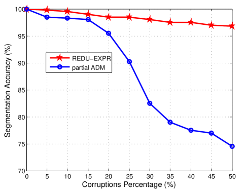
Figure 2: Comparison of accuracies of solutions to relaxed R-LRR (6) computed by REDU-EXPR (Wei and Lin, 2010) and partial ADM (Favaro et al., 2011), where the parameter $\lambda$ is adopted as $1/\sqrt{\log n}$ and $n$ is the input size. The program is run by 10 times and the average accuracies are reported.

To further compare the optimality, we also record the objective function values computed by the two algorithms. Since both algorithms aim at achieving the low rankness of the affinity matrix and the column sparsity of the noise matrix, we compare the objective function of the original R-LRR (5), i.e.,

$$\mathcal{F}(Z,E)=\mbox{rank}(Z)+\lambda||E||_{\ell_{2,0}}.$$ (55)

As shown in Table 4, R-LRR by REDU-EXPR could obtain smaller rank$(Z)$ and objective function than those of partial ADM. Table 4 also shows the CPU times (in seconds). One can see that REDU-EXPR is significantly faster than partial ADM when solving the same model.

Table 4: Comparison of robustness and speed between partial ADM (LRSC) (Favaro et al., 2011) and REDU-EXPR (RSI) (Wei and Lin, 2010) methods for solving R-LRR when the percentage of corruptions increases. All the experiments are run ten times and the $\lambda$ is set to be the same: $\lambda=1/\sqrt{\log n}$, where $n$ is the data size.

Noise Percentage (%)	0	10	20	30	40	50
Rank($Z$) (partial ADM)	20	30	30	30	30	30
Rank($Z$) (REDU-EXPR)	20	20	20	20	20	20
$||E||_{\ell_{2,0}}$ (partial ADM)	0	99	200	300	400	500
$||E||_{\ell_{2,0}}$ (REDU-EXPR)	0	100	200	300	400	500
Objective (partial ADM)	20.00	67.67	106.10	144.14	182.19	220.24
Objective (REDU-EXPR)	20.00	58.05	96.10	134.14	172.19	210.24
Time (s, partial ADM)	4.89	124.33	126.34	119.12	115.20	113.94
Time (s, REDU-EXPR)	10.67	9.60	8.34	8.60	9.00	12.86

6.2 Comparison of Speed on Synthetic Data

In this subsection, we show the great speed advantage of our REDU-EXPR algorithm in solving low rank recovery models. We compare the algorithms to solve relaxed R-LRR (6). We also present the results of solving LRR by ADM for reference, although it is a slightly different model. Except our $\ell_{2,1}$ filtering algorithm, all the codes run in this test are offered by the authors of Liu et al. (2013), Liu and Yan (2011), and Favaro et al. (2011).

The parameter $\lambda$ is set for each method so that the highest accuracy is obtained. We generate clean data as we did in Section 6.1. The only differences are the choice of the dimension of the ambient space and the number of points sampled from subspaces. We compare the speed of different algorithms on corrupted data, where the noises are added in the same way as in (Liu et al., 2010) and (Liu et al., 2013). Namely, the noises are added by submitting to 5% column-wise Gaussian noises with zero means and $0.1||x||_{2}$ standard deviation, where $x$ indicates corresponding vector in the subspace. For REDU-EXPR, with or without using $\ell_{2,1}$ filtering, the rank is estimated at its exact value, twenty, and the over-sampling parameter $s_{c}$ is set to be ten. As the data size goes up, the CPU times are shown in Table 5. When the corruptions are not heavy, all the methods in this test achieve 100% accuracy. We can see that REDU-EXPR consistently outperforms ADM based methods. By $\ell_{2,1}$ filtering, the computation time is further reduced. The advantage of $\ell_{2,1}$ filtering is more salient when the data size is larger.

Table 5: Comparison of CPU time (seconds) between LRR (Liu et al., 2010, 2013) solved by ADM, R-LRR solved by partial ADM (LRSC) (Favaro et al., 2011), R-LRR solved by REDU-EXPR without using $\ell_{2,1}$ filtering (RSI) (Wei and Lin, 2010), and R-LRR solved by REDU-EXPR using $\ell_{2,1}$ filtering as the data size increases. In this test, REDU-EXPR with $\ell_{2,1}$ filtering is significantly faster than other methods and its computation time grows at most linearly with the data size.

Data Size	LRR	R-LRR	R-LRR	R-LRR
	(ADM)	(partial ADM)	(REDU-EXPR)	(filtering REDU-EXPR)
$250\times 250$	33.0879	4.9581	1.4315	0.6843
$500\times 500$	58.9177	7.2029	1.8383	1.0917
$1,000\times 1,000$	370.1058	24.5236	6.1054	1.5429
$2,000\times 2,000$	$>$3600	124.3417	28.3048	2.4426
$4,000\times 4,000$	$>$3600	411.8664	115.7095	3.4253

6.3 Test on Real Data – AR Face Database

Now we test different algorithms on real data, the AR Face database, to classify face images. The AR face database contains 2,574 color images of 99 frontal faces. All the faces are with different facial expressions, illumination conditions, and occlusions (e.g. sun glasses or scarf, see Figure 3), thus the AR database is much harder than the YaleB database for face clustering. So we replace the spectral clustering (Step 3 in Algorithm 2) with a linear classifier. The classification is done as follows:

$$\min_{W}||H-WF||_{F}^{2}+\gamma||W||_{F}^{2},$$ (56)

which is simply a ridge regression and the regularization parameter $\gamma$ is fixed at 0.8, where $F$ is the feature data and $H$ is the label matrix. The classifier is trained as follows. We first run LRR or R-LRR on the original input data $X\in\mathbb{R}^{m\times n}$ and obtain an approximately block diagonal matrix $Z\in\mathbb{R}^{n\times n}$. View each column of $Z$ as a new observation and separate the columns of $Z$ into two parts, where one part corresponds to the training data and the other corresponds to the test data. We train the ridge regression model by the training samples and use the obtained $W$ to classify the test samples.

Figure 3: Examples of images with severe occlusions in the AR database. The images in the same column belong to the same person.

Unlike the existing literatures, e.g., Liu et al. (2010, 2013), which manually removed severely corrupted images and shrank the input images to small-sized ones in order to reduce the computation load, our experiment uses all the full-sized face images. So the size of our data matrix is $19,800\times 2,574$, where each image is reshaped as a column of the matrix, 19,800 is the number of pixels in each image, and 2,574 is the total number of face images. We test LRR (Liu et al., 2010, 2013) (solved by ADM) and relaxed R-LRR (solved by partial ADM (Favaro et al., 2011), REDU-EXPR (Wei and Lin, 2010), and REDU-EXPR with $\ell_{2,1}$ filtering) for both classification accuracy and speed. Table 6 shows the results, where the parameters have been tuned to be the best. Since ADM based method requires too long time to converge, we terminate it after sixty hours. This experiment testifies to the great speed advantage of REDU-EXPR and $\ell_{2,1}$ filtering. Note that with $\ell_{2,1}$ filtering the speed of REDU-EXPR is three times faster than that without $\ell_{2,1}$ filtering, and the accuracy is not compromised.

Table 6: Comparison of classification accuracy and speed on the AR database with the task of face image classification. For fair comparison of both the accuracy and the speed for different algorithms, the parameters are tuned to be the best according to the classification accuracy and we observe the CPU time.

Model	Method	Accuracy	CPU Time (h)
LRR	ADM	-	$>$10
R-LRR	partial ADM	-	$>$10
R-LRR	REDU-EXPR	90.1648%	0.5639
R-LRR	REDU-EXPR with $\ell_{2,1}$ filtering	90.5901%	0.1542

Conclusion and Future Work

In this paper, we investigate the connections among solutions of some representative low rank subspace recovery models, including R-PCA, R-LRR, R-LatLRR, and their convex relaxations. We show that their solutions can be mutually expressed in closed forms. Since R-PCA is the simplest model, it naturally becomes a hinge to all low rank subspace recovery models. Based on our theoretical findings, under certain conditions we are able to find better solutions to low rank subspace recovery models and also significantly speed up finding their solutions numerically, by solving R-PCA first and then express their solutions by that of R-PCA in closed forms. Since there are randomized algorithms for R-PCA, e.g., we propose the $\ell_{2,1}$ filtering algorithm for column sparse R-PCA, the computation complexities for solving existing low rank subspace recovery models can be much lower than the existing algorithms. Extensive experiments on both synthetic and real world data testify to the utility of our theories.

As shown in Section 5.4, our approach may succeed even when the conditions of Section 5.1, 5.2, and 5.3 do not hold. The theoretical analysis on how data distribution influences the success of our approach will be our future work.

Acknowledgments

The authors thank Rene Vidal for valuable discussions. Hongyang Zhang and Chao Zhang are supported by National Key Basic Research Project of China (973 Program) 2011CB302400 and National Nature Science Foundation of China (NSFC grant, no. 61071156). Zhouchen Lin is supported by 973 Program of China (grant no. 2015CB3525), NSF China (grant nos. 61272341 and 61231002), and Microsoft Research Asia Collaborative Research Program. Junbin Gao is supported by the Australian Research Council (ARC) through the grant DP130100364.

References

- Avron et al. (2010) Avron, H., Maymounkov, P., and Toledo, S. (2010). Blendenpik: Supercharging LAPACK’s least-squares solver. SIAM Journal on Scientific Computing, 32(3):1217–1236.
- Basri and Jacobs (2003) Basri, R. and Jacobs, D. (2003). Lambertian reflectance and linear subspaces. IEEE Transactions on Pattern Analysis and Machine Intelligence, 25(2):218–233.
- Belhumeur et al. (1997) Belhumeur, P., Hespanha, J., and Kriegman, D. (1997). Eigenfaces vs. Fisherfaces: Recognition using class specific linear projection. IEEE Transactions on Pattern Analysis and Machine Intelligence, 19(7):711–720.
- Belhumeur and Kriegman (1998) Belhumeur, P. and Kriegman, D. (1998). What is the set of images of an object under all possible illumination conditions? International Journal of Computer Vision, 28(3):245–260.
- Bull and Gao (2012) Bull, G. and Gao, J. (2012). Transposed low rank representation for image classification. In IEEE International Conference on Digital Image Computing Techniques and Application, pages 1–7.
- Candès et al. (2011) Candès, E., Li, X., Ma, Y., and Wright, J. (2011). Robust principal component analysis? Journal of the ACM, 58(3):11.
- Chandrasekaran et al. (2011) Chandrasekaran, V., Sanghavi, S., Parrilo, P., and Willsky, A. (2011). Rank-sparsity incoherence for matrix decomposition. SIAM Journal on Optimization, 21(2):572–596.
- Chen et al. (2011) Chen, Y., Xu, H., Caramanis, C., and Sanghavi, S. (2011). Robust matrix completion and corrupted columns. In International Conference on Machine Learning, pages 873–880.
- Cheng et al. (2011) Cheng, B., Liu, G., Wang, J., Li, H., and Yan, S. (2011). Multi-task low-rank affinity pursuit for image segmentation. In IEEE International Conference on Computer Vision, pages 2439–2446.
- Costeira and Kanade (1998) Costeira, J. and Kanade, T. (1998). A multibody factorization method for independently moving objects. International Journal of Computer Vision, 29(3):159–179.
- De La Torre and Black (2003) De La Torre, F. and Black, M. (2003). A framework for robust subspace learning. International Journal of Computer Vision, 54(1):117–142.
- Elhamifar and Vidal (2009) Elhamifar, E. and Vidal, R. (2009). Sparse subspace clustering. In IEEE Conference on Computer Vision and Pattern Recognition, pages 2790–2797.
- Favaro et al. (2011) Favaro, P., Vidal, R., and Ravichandran, A. (2011). A closed form solution to robust subspace estimation and clustering. In IEEE Conference on Computer Vision and Pattern Recognition, pages 1801–1807.
- Fischler and Bolles (1981) Fischler, M. and Bolles, R. (1981). Random sample consensus: a paradigm for model fitting with applications to image analysis and automated cartography. Communications of the ACM, 24(6):381–395.
- Gear (1998) Gear, W. (1998). Multibody grouping from motion images. International Journal of Computer Vision, 29(2):133–150.
- Gnanadesikan and Kettenring (1972) Gnanadesikan, R. and Kettenring, J. (1972). Robust estimates, residuals, and outlier detection with multiresponse data. Biometrics, 28(1):81–124.
- Golub and Van Loan (2012) Golub, G. and Van Loan, C. (2012). Matrix computations, volume 3. Johns Hopkins University Press.
- Ho et al. (2003) Ho, J., Yang, M., Lim, J., Lee, K., and Kriegman, D. (2003). Clustering appearances of objects under varying illumination conditions. In IEEE Conference on Computer Vision and Pattern Recognition, pages 313–320.
- Hsu et al. (2011) Hsu, D., Kakade, S. M., and Zhang, T. (2011). Robust matrix decomposition with sparse corruptions. IEEE Transactions on Information Theory, 57(11):7221–7234.
- Huber (2011) Huber, P. (2011). Robust statistics. Springer.
- Ji et al. (2010) Ji, H., Liu, C., Shen, Z., and Xu, Y. (2010). Robust video denoising using low-rank matrix completion. In IEEE Conference on Computer Vision and Pattern Recognition, pages 1791–1798.
- Ke and Kanade (2005) Ke, Q. and Kanade, T. (2005). Robust -norm factorization in the presence of outliers and missing data by alternative convex programming. In IEEE Conference on Computer Vision and Pattern Recognition, pages 739–746.
- Lin et al. (2011) Lin, Z., Liu, R., and Su, Z. (2011). Linearized alternating direction method with adaptive penalty for low-rank representation. In Advances in Neural Information Processing Systems, pages 612–620.
- Liu et al. (2013) Liu, G., Lin, Z., Yan, S., Sun, J., and Ma, Y. (2013). Robust recovery of subspace structures by low-rank representation. IEEE Transactions on Pattern Analysis and Machine Intelligence, 35(1):171–184.
- Liu et al. (2010) Liu, G., Lin, Z., and Yu, Y. (2010). Robust subspace segmentation by low-rank representation. In International Conference on Machine Learning, pages 663–670.
- Liu and Yan (2011) Liu, G. and Yan, S. (2011). Latent low-rank representation for subspace segmentation and feature extraction. In IEEE International Conference on Computer Vision, pages 1615–1622.
- Liu et al. (2012) Liu, R., Lin, Z., De la Torre, F., and Su, Z. (2012). Fixed-rank representation for unsupervised visual learning. In IEEE Conference on Computer Vision and Pattern Recognition, pages 598–605.
- Liu et al. (2014) Liu, R., Lin, Z., Su, Z., and Gao, J. (2014). Linear time principal component pursuit and its extensions using filtering. Neurocomputing, 142:529–541.
- Ma et al. (2007) Ma, Y., Derksen, H., Hong, W., and Wright, J. (2007). Segmentation of multivariate mixed data via lossy data coding and compression. IEEE Transactions on Pattern Analysis and Machine Intelligence, 29(9):1546–1562.
- Mahoney (2011) Mahoney, M. W. (2011). Randomized algorithms for matrices and data. Foundations and Trends in Machine Learning, 3(2):123–224.
- Ni et al. (2010) Ni, Y., Sun, J., Yuan, X., Yan, S., and Cheong, L. (2010). Robust low-rank subspace segmentation with semidefinite guarantees. In IEEE International Conference on Data Mining Workshops.
- Paoletti et al. (2007) Paoletti, S., Juloski, A., Ferrari-Trecate, G., and Vidal, R. (2007). Identification of hybrid systems—a tutorial. European Journal of Control, 13(2–3):242–260.
- Peng et al. (2010) Peng, Y., Ganesh, A., Wright, J., Xu, W., and Ma, Y. (2010). RASL: Robust alignment by sparse and low-rank decomposition for linearly correlated images. In IEEE Conference on Computer Vision and Pattern Recognition, pages 763–770.
- Rao et al. (2010) Rao, S., Tron, R., Vidal, R., and Ma, Y. (2010). Motion segmentation in the presence of outlying, incomplete, or corrupted trajectories. IEEE Transactions on Pattern Analysis and Machine Intelligence, 32(10):1832–1845.
- Tomasi and Kanade (1992) Tomasi, C. and Kanade, T. (1992). Shape and motion from image streams under orthography—a factorization method. International Journal of Computer Vision, 9(2):137–154.
- Vidal (2011) Vidal, R. (2011). Subspace clustering. IEEE Signal Processing Magazine, 28(2):52–68.
- Vidal and Favaro (2014) Vidal, R. and Favaro, P. (2014). Low rank subspace clustering. Pattern Recognition Letters, 43:47–61.
- Vidal and Hartley (2004) Vidal, R. and Hartley, R. (2004). Motion segmentation with missing data using PowerFactorization and GPCA. In IEEE Conference on Computer Vision and Pattern Recognition, pages 85–105.
- Vidal et al. (2005) Vidal, R., Ma, Y., and Sastry, S. (2005). Generalized principal component analysis (GPCA). IEEE Transactions on Pattern Analysis and Machine Intelligence, 27(12):1945–1959.
- Vidal et al. (2003) Vidal, R., Soatto, S., Ma, Y., and Sastry, S. (2003). An algebraic geometric approach to the identification of a class of linear hybrid systems. In IEEE International Conference on Decision and Control, pages 167–172.
- Wang et al. (2009) Wang, J., Dong, Y., Tong, X., Lin, Z., and Guo, B. (2009). Kernel Nystrm method for light transport. ACM SIGGRAPH, pages 1–10.
- Wang et al. (2011) Wang, J., Saligrama, V., and Castan, D. (2011). Structural similarity and distance in learning. In Annual Allerton Conference on Communication, Control, and Computing, pages 744–751.
- Wei and Lin (2010) Wei, S. and Lin, Z. (2010). Analysis and improvement of low rank representation for subspace segmentation. http://arxiv.org/abs/1107.1561.
- Wright et al. (2009) Wright, J., Ganesh, A., Rao, S., Peng, Y., and Ma, Y. (2009). Robust principal component analysis: Exact recovery of corrupted low-rank matrices via convex optimization. In Advances in Neural Information Processing Systems, pages 2080–2088.
- Xu et al. (2012) Xu, H., Caramanis, C., and Sanghavi, S. (2012). Robust PCA via outlier pursuit. IEEE Transaction on Information Theory, 58(5):3047–3064.
- Yan and Pollefeys (2006) Yan, J. and Pollefeys, M. (2006). A general framework for motion segmentation: Independent, articulated, rigid, non-rigid, degenerate and nondegenerate. In European Conference on Computer Vision, volume 3954, pages 94–106.
- Yang et al. (2008) Yang, A., Wright, J., Ma, Y., and Sastry, S. (2008). Unsupervised segmentation of natural images via lossy data compression. Computer Vision and Image Understanding, 110(2):212–225.
- Zhang and Bitmead (2005) Zhang, C. and Bitmead, R. (2005). Subspace system identification for training-based MIMO channel estimation. Automatica, 41(9):1623–1632.
- Zhang et al. (2013a) Zhang, H., Lin, Z., and Zhang, C. (2013a). A counterexample for the validity of using nuclear norm as a convex surrogate of rank. In European Conference on Machine Learning and Principles and Practice of Knowledge Discovery in Databases, volume 8189, pages 226–241.
- Zhang et al. (2015) Zhang, H., Lin, Z., Zhang, C., and Chang, E. (2015). Exact recoverability of robust PCA via outlier pursuit with tight recovery bounds (to appear). In AAAI Conference on Artificial Intelligence.
- Zhang et al. (2014) Zhang, H., Lin, Z., Zhang, C., and Gao, J. (2014). Robust latent low rank representation for subspace clustering. Neurocomputing, 145:369–373.
- Zhang et al. (2013b) Zhang, Y., Jiang, Z., and Davis, L. (2013b). Learning structured low-rank representations for image classification. In IEEE Conference on Computer Vision and Pattern Recognition, pages 676–683.
- Zhang et al. (2012) Zhang, Z., Ganesh, A., Liang, X., and Ma, Y. (2012). TILT: Transform-invariant low-rank textures. International Journal of Computer Vision, 99(1):1–24.