JET BENDING AND VELOCITY PROFILES

Abstract

In this study, we consider the problem of geometry of curved jets. We work with a simplified two-dimensional kinematical model assuming that the jet velocity is varying. We prescribe the velocity variation and study two cases concerning parsec and kilo-parsec scale jets by applying some simplified numerical simulations. For parsec scale jets, we use some general expressions and derive the shape of jets for certain numerical cases. For kilo-parsec scale jets, we study the cases of 4C53.37 and 1159+583 of Abell 2220 and Abell 1446 galaxy clusters, respectively, in an effort to test our model and compare our numerical results with observational data.

Keywords: galaxies: jets (bending, parsec scale, kilo-parsec scale, velocity variation); individual objects (4C53.37, 1159+583, Abell 2220, Abell 1446)

1 Introduction

Jets are an interesting issue in astrophysics. We know how they are produced and propagate through space, but there are still some questions regarding their interaction with their environment. In theory, galactic jets seem to be streams of plasma directed perpendicular to an accretion disk surrounding a supermassive black hole. Observations reveal curved jets. Such jet bending is due to the interaction of the jet with a nebula, a gas cloud, a density anisotropy, or any other cause that can be expressed as a pressure gradient while the jet is journeying through the galactic center or the intergalactic medium.

The bending of a jet depends on its velocity and on the external pressure gradient ([1], Secs. I and III). Assuming that (i) the pressure gradient is distance-dependent ([2], Fig. 5.4),

$$P=\,\frac{P_{0}}{1+y^{2}/y^{2}_{0}}\,,$$ (1)

where $P_{0}$ and $y_{0}$ are model parameters, and that (ii) this behaviour is the same for any jet, then the difference in jet bending is due to the velocity profile.

Even though small scale jets are usually considered to be accelerating to speeds near the speed of light, velocities for parsec and kilo-parsec scales are of order $\sim 10^{3}\,\mathrm{km\,s^{-1}}$ (cf. [3], Table 1); and they are generally considered constant. For galactic jets owing to AGN, which can reach lengths of up to a few mega-parsecs, it is probably of lower significance to consider time-varying velocities. Still, given the scales involved, we cannot assume that they are constant, especially when their interaction with the pressure gradient is taken into account. Accordingly, we have to examine two scenarios: either an accelerating jet, until it becomes relativistic or destroyed after interacting with an external pressure, or a decelerating one.

2 Jet Model

For our jet model, we adopt a two-dimensional kinematical model ([2], Eq. 5.17; we use here the definitions and symbols of this investigation),

$$\frac{d^{2}f}{dx^{2}}\,\left[1+\left(\frac{df}{dx}\right)^{2}\right]^{-3/2}=\,\frac{1}{\rho u^{2}}\,\,\frac{\partial P}{\partial R}|_{\perp},$$ (2)

where ([2], Eq. 5.18)

$$\frac{\partial P}{\partial R}|_{\perp}=\sin(a)\,\,\frac{\partial P}{\partial x}\,-\,\cos(a)\,\,\frac{\partial P}{\partial y},$$ (3)

with ([2], Eq. 5.19)

$$\tan(a)=\,\frac{df}{dx}.$$ (4)

Assuming that the pressure gradient is a function of the $y$-coordinate, we obtain the dimensionless form ([2], Eq. 5.22)

$$x=x_{0}+\int^{y}_{0}\left[L\,e^{-2P(f)/\rho\,u^{2}}-1\right]^{-1/2}\,df,$$ (5)

where $x_{0}$ is the integration constant and $L$ a parameter associated with the angle the jet meets the pressure gradient ([2], Eq. 5.23),

$$\tan(i)=\left(L-1\right)^{-1/2}.$$ (6)

There is a critical value $L_{\mathrm{crit}}$ ([2], remarks following Eq. (5.27) and Fig. 5.5), such that, when below that value, the jet stops propagating forward and returns towards its source.

3 The Computations

To compile our code, we use the gfortran compiler, licensed under the GNU General Public License (GPL; http://www.gnu.org/licenses/gpl.html). gfortran is the name of the GNU Fortran compiler belonging to the GNU Compiler Collection (GCC; http://gcc.gnu.org/). In our computer, it has been installed by the TDM-GCC “Compiler Suite for Windows” (http://tdm-gcc. tdragon.net/), which is free software distributed under the terms of the GPL. Subroutines required for standard numerical procedures are taken from the SLATEC Common Mathematical Library, which is an extensive public-domain Fortran Source Code Library, incorporating several public-domain packages. The full SLATEC release is available in http://netlib.org/slatec/. In particular, to compute integrals we use the subroutine DGAUS8, which integrates real functions in one variable along finite intervals on the basis of an adaptive 8-point Legendre-Gauss algorithm, and which is appropriate for high accuracy integrations.

4 Parsec and Kilo-parsec Scale Jets

After some preliminary tests of the code, we examine four different cases for the velocity profile. Two cases have to do with an accelerating jet (linear and nonlinear), and further two with a decelerating one (linear and nonlinear). For the nonlinear case we adopt a simplified exponential behaviour,

$$u=u_{0}\,\mathrm{exp}(\pm y).$$ (7)

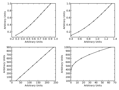
Figure 1: Velocity profiles corresponding to four cases. Top left: accelerating exponentially. Top right: accelerating linearly. Bottom left: decelerating exponentially. Bottom right: decelerating linearly.

We examine several velocity profiles and scales for all cases and show their graphs in Fig. 1. Regarding the form we expect to have for this model, it is clear that the jets must be decelerating linearly, a conclusion also derived in [4] (Sec. 3.3). With that result in mind, we proceed in examining the cases for parsec and kilo-parsec scale jets.

4.1 Parsec scale jets

In the case of parsec scale jets, we assume that the bending is caused by an external pressure gradient interacting with the jet while moving through the galactic center. We examine sixteen different sets of parameters. In detail, we introduce four “velocity coefficients”, $\lambda_{1}=0.1$, $\lambda_{2}=0.4$, $\lambda_{3}=0.7$, $\lambda_{4}=1.0$, in order for the velocity to vary from one to two orders of magnitude ([4], Sec. 4)

$$u_{i}=u_{0}-\lambda_{i}\,y$$ (8)

In addition, for each velocity coefficient $\lambda_{i}$, we use four values of the parameter $L$, $L_{1}=2.718$, $L_{2}=4$, $L_{3}=6.8482$, $L_{4}=10.475$, corresponding to angles $i_{1}=\pi/2$, $i_{2}=\pi/4$, $i_{3}=\pi/8$, and $i_{4}=\pi/10$, respectively. Numerical experiments with several angles show that these particular values lead to distinguishable graphs (since close angles yield almost identical curves).

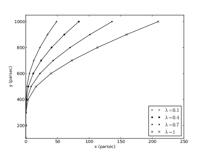
Figure 4: Jet paths with interaction constant $L=6.8284$ for all velocity coefficients $\lambda_{i}$.

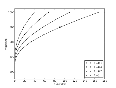
Figure 5: Jet paths with interaction constant $L=10.472$ for all velocity coefficients $\lambda_{i}$.

Numerical results for $\lambda_{1}=0.1$ and $\lambda_{2}=0.4$ are given in Table 1; and for $\lambda_{3}=0.7$, $\lambda_{4}=1.0$ in Table 2. Grouping according to the interaction angle, Fig. 2 shows the case $L_{1}=2.718$, Fig. 3 the case $L_{2}=4$, Fig. 4 the case $L_{3}=6.8482$, and Fig. 5 deals with the case $L_{4}=10.472$. All $X$ and $Y$ values are given in pc.

We can see how the velocity affects the shape of the jet, and how the interaction angle affects the final length of the jet. Moreover , in all cases computed, all values $X$ corresponding to $Y=100$ pc are of order(s) below the accuracy of the computations, so considered to be zero. All $X$ values corresponding to $Y=200$ pc are of order(s) $10^{-4}$—$10^{-6}$. These values correspond to a diversion of approximately $10^{7}$—$10^{9}$ km; even thought it is very small compared to the scale of the jets, it cannot be neglected. We can conclude that the bending of the jet begins at a distance between 100 pc and 200 pc from the source.

Knowing the speed of the jet, and reducing observational data to scale, we can draw information and conclusion about the velocity variation and interaction angle.

4.2 Kilo-parsec scale jets

We consider the well-known jets of the structures 4C53.37 and 1159+583 in the galaxy clusters Abell 2220 and Abell 1446, respectively. The bending of the jets is now due to the relative movement of the galaxy through the “intercluster medium” (ICM). Since, in this case, we have a much larger scale (hundreds of kilo-parsecs), we adopt a nonrelativistic hydrodynamic expression for the velocity given by the Euler equation

$$\frac{\partial u}{\partial t}+(u\nabla)u=\,-\,\frac{\nabla P}{\rho}+g.$$ (9)

Following a similar analysis as before, the expression for the velocity becomes ([6], Eq. (7); we use here the definitions and symbols of this investigation)

$$u=\left[\frac{6\,R\,k\,T\,n_{0}\,r}{\rho_{t}\,r_{c}^{2}\,\left(1+r^{2}/r_{c}^{2}\right)^{5/2}}+\,\frac{2\,R\,U^{2}_{\mathrm{gal}}\,m_{p}\,n_{0}}{\rho_{t}\,r_{t}\,\left(1+r^{2}/r_{c}^{2}\right)^{3/2}}\right]^{1/2},$$ (10)

Burns and Balonek ([6], Eq. (9)) have managed to reduce Eq. (10) to the form

$$u_{j}=U_{\mathrm{gal}}\,\left(\frac{n_{\mathrm{ICM}}}{n_{j}}\,\frac{2\,R}{h}\right)^{1/2},$$ (11)

where $u_{j}$ and $n_{j}$ are the velocity and density of the jet, $U_{\mathrm{gal}}$ the velocity of the host galaxy, $n_{\mathrm{ICM}}$ the mean intercluster density, $R$ the radius of curvature, and $h$ the distance from the source at which the interaction with the pressure gradient begins (scale height). For the case of ICM with high density, $h$ is equal to the radius of the galactic center; for the case of ICM with low density, on the other hand, $h$ coincides with the length of the jet.

Using parameters given in [6] (Secs. III, IV), we plot three different values of the density ratio $n=n_{ICM}/n_{j}$ for each jet. Results for 4C53.37 and 1159+583 are shown in Table 3 and in Figs. 6 and 7, respectively.

The observational values for $n$ in [6] are $n=0.5$ for 4C53.37, and $n=12$ for 1159+583. Figs. 6 and 7 show how the shape of the jet does change with different intercluster densities. For the case of 4C53.37 there is a formidable variation in the shape of the curves between density ratios, whereas for the case of 1159+583 the differences are small. Comparing our results with observational data given by [7] and [8] for 4C53.37 and 1159+583, respectively, and taking into account only the main jet, even though the jet in 4C53.37 seems to have lost its shape, if we imagine the path it would have followed, both jets seem to be in agreement with our computations.

5 Conclusions

Approximating a two dimensional kinematical model by some simplified simulations, we have studied the velocity profiles of large scale jets by assuming that their speed is not constant. We have seen that, when the velocity of the jet decreases linearly, the angle of interaction affects the length of the jet; and the bending begins at distances over 100 pc from the source. Regarding kilo-parsec scale jets, we can say that, morphologically, our simplified numerical simulations give results resembling relevant observations.

Table 1: Calculated values with velocity coefficients $\lambda=0.1$ and $\lambda=0.4$ for all interaction constants. $X$ and $Y$ are given in pc.

$X_{L_{1}}$	$X_{L_{2}}$	$X_{L_{3}}$	$X_{L_{4}}$	$X_{L_{1}}$	$X_{L_{2}}$	$X_{L_{3}}$	$X_{L_{4}}$	Y
$10^{-6}$	8$\times 10^{-7}$	6$\times 10^{-7}$	5$\times 10^{-7}$	5$\times 10^{-6}$	4$\times 10^{-6}$	3$\times 10^{-6}$	2$\times 10^{-6}$	200
0.012	0.01	0.007	0.006	0.039	0.032	0.025	0.02	300
0.46	0.379	0.290	0.234	1.165	0.96	0.735	0.593	400
2.983	2.459	1.881	1.519	6.590	5.43	4.154	3.354	500
9.339	7.695	5.886	4.752	18.924	15.578	11.909	9.611	600
20.261	16.681	12.753	10.293	38.739	31.84	24.307	19.603	700
35.655	29.326	22.402	18.073	65.413	53.661	40.099	32.958	800
55.059	45.234	34.520	27.836	97.950	80.191	61.015	49.128	900
77.916	63.935	48.741	39.283	135.343	110.588	84.002	67.583	1000

Table 2: Calculated values with velocity coefficients $\lambda=0.7$ and $\lambda=1$ for all interaction constants. Details as in Table 1.

$X_{L_{1}}$	$X_{L_{2}}$	$X_{L_{3}}$	$X_{L_{4}}$	$X_{L_{1}}$	$X_{L_{2}}$	$X_{L_{3}}$	$X_{L_{4}}$	Y
2.8$\times 10^{-5}$	2.3$\times 10^{-5}$	1.7$\times 10^{-5}$	1.4$\times 10^{-5}$	1.2$\times 10^{-4}$	$\times 10^{-4}$	8$\times 10^{-5}$	6$\times 10^{-5}$	200
0.11	0.098	0.075	0.06	0.326	0.269	0.206	0.166	300
2.73	2.256	1.726	1.394	5.974	4.922	3.766	3.04	400
13.559	11.165	8.537	6.89	26.086	21.445	16.374	13.207	500
35.89	29.488	22.506	18.148	63.989	52.396	39.871	32.106	600
69.59	57.017	43.408	34.961	117.964	96.157	72.893	58.599	700
113.080	92.356	70.127	56.411	184.833	150.027	113.330	90.939	800
164.509	133.962	101.468	81.524	261.536	211.517	159.302	127.648	900
222.235	180.489	136.406	109.48	345.606	278.676	209.367	167.571	1000

Table 3: Calculated values with three different density ratios. For 4C53.37: $n_{1}=0.1$, $n_{2}=0.5$, $n_{3}=1$. For 1159+583: $n_{4}=5$, $n_{5}=9$, $n_{6}=12$. Details as in Table 1.

$X_{n_{1}}$	$X_{n_{2}}$	$X_{n_{3}}$	$X_{n_{4}}$	$X_{n_{5}}$	$X_{n_{6}}$	Y
0.408	1.3$\times 10^{-6}$	0	0.016	8$\times 10^{-5}$	$10^{-6}$	150
4.933	0.013	$10^{-5}$	1.341	0.116	0.02	200
15.907	0.513	0.014	8.893	2.161	0.813	250
31.672	3.259	0.342	25.256	9.862	5.245	300
50.274	9.743	2.059	49.364	24.876	15.875	350
70.445	20.087	6.387	79.265	46.633	33.135	400
91.460	33.656	13.858	113.227	73.832	56.233	450
112.886	49.679	24.357	149.956	105.178	84.056	500
134.498	67.485	37.457	188.549	139.585	115.551	550
156.178	86.557	52.663	228.361	176.221	149.828	600

Figure 2: Jet paths with interaction constant $L=2.718$ for all velocity coefficients $\lambda_{i}$.

Figure 3: Jet paths with interaction constant $L=4$ for all velocity coefficients $\lambda_{i}$.

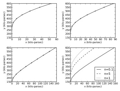
Figure 6: Jet paths for three density ratios. Top left: $n=1$. Top right: $n=0.5$. Bottom left: $n=0.1$. Bottom right: all $n$ values.

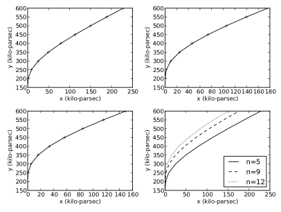
Figure 7: Jet paths for three density ratios. Top left: $n=5$. Top right: $n=9$. Bottom left: $n=12$. Bottom right: all $n$ values.

References

- [1] R. Fiedler and R. N. Henriksen, The Astrophysical Journal, 281, 554-559 (1984).
- [2] V. Icke, “From nucleus to hotspot: nine powers of ten”. In “Beams and Jets in Astrophysics”, P. A. Hughes (ed.), Cambridge University Press, 242, 232-277 (1991).
- [3] G. Pelletier and H. Sol, Monthly Notices of the Royal Astronomical Society, 254, 635-646 (1992).
- [4] D. S. De Young, The Astrophysical Journal, 371, 69-81 (1991).
- [5] A. P. Marscher, “Relativistic Jets in Active Galactic Nuclei”, American Institute of Physics Conference Series, P. A. Hughes & J. N. Bregman (eds.), Vol. 856, pp. 1-22 (2006).
- [6] J. O. Burns and T. J. Balonek, The Astrophysical Journal, 263, 546-556 (1982).
- [7] J. O. Burns and F. N. Owen, The Astronomical Journal, 85(3), 204-214 (1980).
- [8] J. O. Burns, F. N. Owen, and L. Rudnick, The Astronomical Journal, 84(11), 1683-1693 (1979).