Discovery of a periodical apoastron GeV peak in LS I $+61^{\circ}303$

Abstract

Aims. The aim of this paper is to analyse the previously discovered discontinuity of the periodicity of the GeV $\gamma$-ray emission of the radio-loud X-ray binary LS I $+61^{\circ}303$ and to determine its physical origin.

Methods. We used wavelet analysis to explore the temporal development of periodic signals. The wavelet analysis was first applied to the whole data set of available Fermi-LAT data and then to the two subsets of orbital phase intervals $\Phi=0.0-0.5$ and $\Phi=0.5-1.0$. We also performed a Lomb-Scargle timing analysis. We investigated the similarities between GeV $\gamma$-ray emission and radio emission by comparing the folded curves of the Fermi-LAT data and the Green Bank Interferometer radio data.

Results. During the epochs when the timing analysis fails to determine the orbital periodicity, the periodicity is present in the two orbital phase intervals $\Phi=0.0-0.5$ and $\Phi=0.5-1.0$. That is, there are two periodical signals, one towards periastron (i.e., $\Phi=0.0-0.5$) and another one towards apoastron ($\Phi=0.5-1.0$). The apoastron peak seems to be affected by the same orbital shift as the radio outbursts and, in addition, reveals the same two periods $P_{1}$ and $P_{2}$ that are present in the radio data.

Conclusions. The $\gamma$-ray emission of the apoastron peak normally just broadens the emission of the peak around periastron. Only when it appears at $\Phi\approx 0.8-1.0$, because of the orbital shift, it is enough detached from the first peak to become recognisable as a second orbital peak, which is the reason why the timing analysis fails. Two $\gamma$-ray peaks along the orbit are predicted by the two-peak accretion model for an eccentric orbit, that was proposed by several authors for LS I $+61^{\circ}303$.

1 Introduction

The system LS I $+61^{\circ}303$ with an orbital period  $P_{1}=26.4960\pm 0.0028\,\mathrm{days}$ (Gregory 2002) consists of a compact object and a massive star with an optical spectrum typical for a rapidly rotating B0 V star (Casares et al. 2005; Grundstrom et al. 2007).

In 2009 the first detection of orbital periodicity in high-energy gamma rays (20 MeV–100 GeV) was reported by using the Large Area Telescope (LAT) from the Fermi Gamma-Ray Space Telescope spacecraft (Abdo et al. 2009). Longer monitoring has shown (Hadasch et al. 2012; Ackermann et al. 2013) that indeed the system shows a clear periodical outburst towards periastron ($\Phi_{\rm periastron}=0.23$, Casares et al. 2005) at some epochs, but that this periodicity is not always present. This is different from the behaviour of the system in the radio band where not only periodical outbursts occur at each orbit, even if modulated with a long-term period ($P_{\rm long}$ = 1667 $\pm$ 8 d, Gregory 2002), but they also occur towards apoastron and not towards periastron as in the GeV energy band (e.g., see Fig. 2 c in Massi & Kaufman Bernadó 2009).

Along with this different behaviour between high and low energy there is a puzzling overlap. Ackermann et al. (2013) noticed that GeV data also show the long-term periodical variation affecting the radio data, but only at a specific orbital phase interval, $\Phi=0.5-1.0$, that is around apoastron.

The aim of this paper is to investigate the discontinuity in the periodicity of the GeV $\gamma$-ray emission at periastron, the relationship of its disappearance with the variation of the emission in other parts of the orbit, and finally the possible relationship between GeV and radio emission. Section 2 describes our data analysis. In Sect. 3 we present our results and in Sect. 4 our conclusions.

2 Data analysis

In this section we present the data reduction of Fermi-LAT data performed with three packages: the Fermi science tools package (version v9r33p0), the wavelet analysis, and the software Starlink.

The $\gamma$-ray data used in this analysis span the time period MJD 54683 (August 05, 2008) to MJD 56838 (June 30, 2014). We used the script like_lc.pl by Robin Corbet. Only source-event-class photons were selected for the analysis. Photons with a zenith angle greater than 100^∘ were excluded to reduce contamination from the Earth’s limb. For the diffuse emission we used the model gll_iem_v05_rev1.fit and the template iso_source_v05_rev1.txt. We used the instrument response function (IRF) P7REP/background_rev1, and the model file was generated from the 2FGL catalogue (Nolan et al. 2012), all sources within $10^{\circ}$ of LS I $+61^{\circ}303$ were included in the model. LS I $+61^{\circ}303$ was fitted with a log-parabola spectral shape and with all parameters left free for the fit, performing an unbinned maximum likelihood analysis. The other sources were fixed to their catalogue values. We produced light curves with a time bin size of one day and of five days. For all light curves we used an energy range of 100 MeV to 300 GeV.

The data were folded with the orbital phase defined as

$$\Phi=\frac{t-t_{0}}{P_{1}}-{\rm int}\left(\frac{t-t_{0}}{P_{1}}\right),$$ (1)

where $t_{0}=43366.275\,\mathrm{MJD}$ and $P_{1}=26.4960\pm 0.0028\,\mathrm{d}$ is the orbital period of the binary system (Gregory 2002).

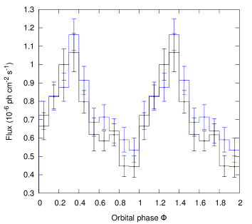
Figure 1: Folded light curve (blue) of Fig. 8 by Hadasch et al. (2012). This covers the first 8 months of Fermi-LAT observations. As comparison we give our folded data (black) from the same time interval. This time interval corresponds to $\Theta=6.79-6.92$.

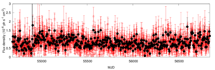
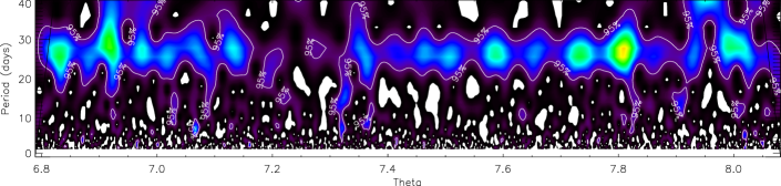
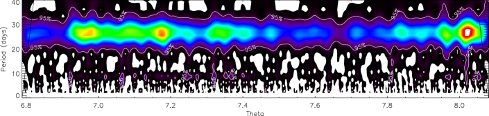
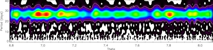
Figure 2: Wavelet analysis of Fermi-LAT data. The strength of periodicity is colour coded as indicated in the bottom bar. (a) Fermi-LAT data with a time bin of 5 d (black) are overplotted on Fermi-LAT data with a time bin of 1 d (red). The black line marks the point of flux change reported by Hadasch et al. (2012) which is also visible in our light curve. (b) Wavelet analysis for the whole data set, that is for the whole orbital interval $0.0-1.0$ (b–d use a time bin of one day). (c) Wavelet analysis for half the data set, that is for the orbital interval $\Phi=0.5-1.0$, i.e., around apoastron. (d) Wavelet for half the data set, that is for the orbital interval $\Phi=0.0-0.5$, i.e., around periastron.

We investigated the temporal evolution of the orbital periodicity by means of a wavelet analysis with Morlet function (Torrence & Compo 1998). The wavelet analysis decomposes the one-dimensional time series into a two-dimensional time-frequency space and displays the power spectrum in a two-dimensional colour-plot that shows how the Fourier periods vary in time (Torrence & Compo 1998). While the wavelet analysis was applied to the $\gamma$-ray data vs time, for a straightforward comparison with radio data, we express the $x$-axis as

$$\Theta=\frac{t-t_{0}}{P_{\rm long}}.$$ (2)

This allows a comparison with non-simultaneous radio data because the radio data are periodical in $\Theta$. We will therefore compare gamma-ray data to radio data having the same fractional part of $\Theta$. For the Lomb-Scargle timing analysis (Lomb 1976; Scargle 1982), we used the program PERIOD, which is part of the UK software Starlink. The version we used was 5.0-2 for UNIX. The wavelet analysis assumes regularly sampled data. We therefore set the data for the wavelet analysis to zero for missing flux. For the Lomb-Scargle analysis this was not necessary. As discussed in Sect. 3, the Lomb-Scargle analysis confirms and accurately determins the periodicities found with the wavelet analysis. In the Lomb-Scargle and wavelet analysis, significance levels for the spectra were determined with the Fisher randomisation, as outlined in Linnell Nemec & Nemec (1985), and with Monte Carlo simulations, as in Torrence & Compo (1998). The fundamental assumption is: if there is no periodic signal in the time series data, then the measured values are independent of their observation times and are likely to have occurred on any other order. One thousand randomized time-series were formed and the periodograms calculated. The proportion of permutations that give a peak power higher than that of the original time series would then provide an estimate of $p$, the probability that for a given frequency window there is no periodic component present in the data with this period. A derived period is defined as significant for $p<0.01$, and a marginally significant period for $0.01<p<0.10$ (Linnell Nemec & Nemec 1985).

3 Results

In this section we discuss our wavelet and Lomb-Scargle results for the gamma-ray data and compare them with previously published results (Hadasch et al. 2012; Ackermann et al. 2013). Then we compare gamma-ray data with radio data.

3.1 Wavelet and Lomb-Scargle analysis

As a general check of our data reduction we verified the consistency of the folded curve of our data with the folded curve of Hadasch et al. (2012). For this purpose we selected the same time interval as in Hadasch et al. (2012), that is 54683–54900 MJD ($\Theta=6.79-6.92$), covering the first eight months of Fermi-LAT observations. Figure 1 presents the result by Hadasch et al. (2012) and our results. We see how these independently calibrated data sets, which used different versions of the software, of the instrumental response funtion, etc., produce the same result: There is a main peak at orbital phase $\Phi\approx 0.35$.

We compare the light curve and wavelet results with previous results. The whole interval of the Fermi-LAT data used in our analysis is presented in Fig. 2 a. The point of flux change reported by Hadasch et al. (2012) is also visible in our light curve. Figure 2 b shows the wavelet analysis results for the whole data set. The orbital periodicity shows a minimum around $\Theta\approx 7.25$. This agrees with the periodograms of Fig. 7 in Hadasch et al. (2012), where the orbital periodicity is already almost absent for MJD 55044-55225 ($\Theta=7.00-7.11$) and is completely absent at MJD 55405-55586 ($\Theta=7.22-7.33$). The panels of Fig. 4 in Ackermann et al. (2013) show the decline in the orbital flux modulation in the interval MJD 55191–55698 ($\Theta=7.1-7.5$). Our Figs. 1, 2 a and 2 b therefore confirm the orbital modulation that peaks around periastron, the point of flux change at $\Theta\approx 6.95$, and the lack of orbital flux modulation at $\Theta\approx 7.25$ previously discovered and discussed in Hadasch et al. (2012) and Ackermann et al. (2013).

Now we examine the new results obtained when the wavelet analysis is performed separately for emission around periastron, $\Phi=0.0-0.5$, and emission around apoastron, $\Phi=0.5-1.0$. By comparing Fig. 2 d with Fig. 2 c it is clear that the orbital periodicity is not a characteristic of periastron emission alone, it is also present at apoastron, at least at some $\Theta$s. At $\Theta\approx 7.2$ where the wavelet analysis for the whole data set (Fig. 2 b) shows the minimum power for the orbital periodicity, a maximum is present in Fig. 2 c. Orbital flux modulation is present from $\Theta\approx$ 6.95 to $\Theta\approx$ 7.40, and at $\Theta\approx 7.95$ the periodicity is strong again, indicating a repetition consistent with the long-term period $P_{\rm long}$. This confirms the discovery of Ackermann et al. (2013) that in the orbital phase interval $\Phi=0.5-1.0$ the $\gamma$-ray flux shows periodical variation with a period equal to the long-term modulation affecting the radio outburst. In addition, our wavelet analysis shows that the emission at apoastron, affected by the long-term modulation, is orbitally modulated.

We checked the presence of the orbital and long-term periodicities that were indicated by the wavelet analysis with the Lomb-Scargle timing analysis of the data from $\Phi=0.5-1.0$. First of all, the periodogram of the subset $\Phi=0.5-1.0$, shown in Fig. 3 d, presents a periodicitiy at $1705\pm 355$ days, confirming the result of Ackermann et al. (2013) of a long-term modulation of emission around apoastron. Moreover, the periodogram shows a feature at the orbital period $P_{1}$, confirming the results of the wavelet analysis, and this feature seems to have a complex profile. The zoomed version is presented in Fig. 3 e. Figure 3 f shows the periodogram for data integrated over five days. There is one peak at $P_{1}=26.48\pm 0.08\,\mathrm{d}$ and another one at $P_{2}=26.99\pm 0.08\,\mathrm{d}$. When we consider the whole data set, which is the longest time interval of Fermi-LAT data analysed so far, $P_{\rm long}$ and $P_{2}$ are significant in the randomisations tests (i.e., the probability $p$ that there is no periodic component present in the data with these periods is for both periods $p<0.01$), even if they are rather weak features in the periodograms of Fig. 3 a, b, and c. For the emission around periastron, Figures 3 g, h, and i show the Lomb-Scargle periodograms of $\Phi=0.0-0.5$. Here the only outstanding feature is $P_{1}$.

Figure 3: Lomb-Scargle periodogram of the Fermi-LAT (with a time bin of one day). (a) Full data set: data in the orbital phase $\Phi=0.0-1.0$. (b) Zoom of Fig. 3 a. (c) Same as 3 b for data with a time bin of 5 d. The false alarm probability ($p$) resulting from randomisation tests is indicated. A period is defined as significant for $p<1\%$, and as marginally significant for $1\%<p<10\%$ (Sect. 2). (d) Half the data set: data in the orbital phase $\Phi=0.5-1.0$. The periods $P_{2}$ and $P_{\rm long}$ here present are typical periodicities in radio data (Massi & Jaron 2013). (e) Zoom of Fig. 3 d. (f) Same as 3 e for data with a time bin of 5 d. (g) Half the data set: data in the orbital phase $\Phi=0.0-0.5$. (h) Zoom of Fig. 3 g. (i) Same as 3 h for data with a time bin of 5 d.

3.2 Orbital shift

Why does the timing analysis reveal a lack of orbital modulation around $\Theta\approx 7.2$ with a peak at periastron passage when the periodicity is still present, as shown in Fig. 2 d for data at $\Phi=0.0-0.5$? And why does the orbital modulation of GeV emission towards apoastron get stronger in that $\Theta$-interval (Fig. 2 c)? Clearly, the second question is the answer to the first. Two peaks along the orbit disturb the timing analysis. The curves shown in Fig. 4 a, b, and c refer to the three consecutive $\Theta$-intervals around the minimum of Fig. 2 b, that is around the peak of Fig. 2 c: $\Theta=7.12-7.22$ (MJD 55235–55402), $\Theta=7.22-7.32$ (MJD 55402–55569), and $\Theta=7.32-7.42$ (MJD 55569–55743). In addition to the peak at periastron Fig. 4 a and Fig. 4 b show a second peak in the interval $\Phi=0.8-1.0$.

The real question therefore is why periodical emission towards apoastron is detected only at $\Theta\approx 7.2$. The important information from the Lomb-Scargle analysis is that there are two periods, $P_{1}$ and $P_{2}$, as is for radio data (Massi & Jaron 2013). We therefore examined the trend of radio data in that particular $\Theta$-interval. Figure 4 d shows the GBI data at 8 GHz at $\Theta=4.23-4.40$. The curve shows indeed a peak at $\Phi\approx 0.9$ consistent with the second peak in the GeV data in the interval $\Phi=0.8-1.0$ (Fig. 4 a-b). Figure 4 d also shows data at $\Theta=3.79-3.92$, as the GeV data of our Fig. 1. In this case, the radio data show a peak at $\Phi\approx 0.65$ consistent with the bump of emission at $\Phi\approx 0.65$ in the gamma-ray data of Fig. 1. This is the well-known phenomenon of the orbital shift of the radio outburst in LS I $+61^{\circ}303$: The largest outbursts occur at orbital phase 0.6, afterwards, with the long-term periodicity, the orbital phase of the peak of the outburst changes, as analysed by Paredes et al. (1990) in terms of orbital phase shift, by Gregory et al. (1999) in terms of timing residuals, and reproduced recently by the precessing jet model in Massi & Torricelli-Ciamponi (2014; their Fig. 4 b).

The second $\gamma$-ray peak, clearly associated with the radio outburst in terms of timing analysis, therefore also follows the same orbital shift. The second peak is therefore only detected at $\Theta\approx 7.2$, although the periodicity is indeed always present, because in that $\Theta$-interval the peak is detached enough from the first $\gamma$-ray peak to be discernable in the timing analysis.

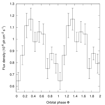
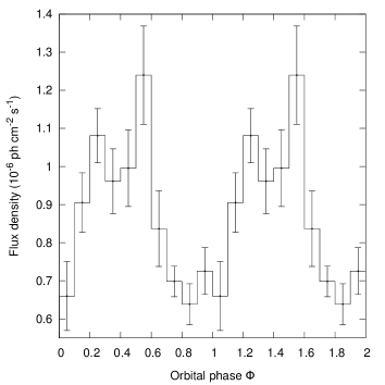
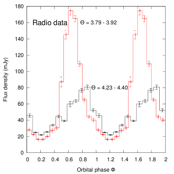
Figure 4: Apoastron peak. Fermi-LAT gamma-ray data folded with the orbital periodicity $P_{1}=26.4960\,\mathrm{d}$ for three consecutive $\Theta$-intervals. (a) $\Theta=7.12-7.22$ (MJD 55235–55402); (b) $\Theta=7.22-7.32$ (MJD 55402–55569); (c) $\Theta=7.32-7.42$ (MJD 55569–55740). (d) GBI radio data at 8 GHz folded with orbital period $P_{1}=26.4960\,\mathrm{d}$. The two $\Theta$-intervals are those considered in Fig. 1 and in this figure for Fermi-LAT data. The orbital phase of the peak of the two radio curves agrees well with those of the second peak in GeV curves.

4 Discussion and conclusion

The first eight months of the Fermi-LAT observations ($\Theta=6.79-6.93$) analysed by Hadasch et al. (2012) indicate a peak of GeV $\gamma$-ray emission close to periastron. This clear orbital modulation of the GeV gamma-ray emission is lost at some time interval (Hadasch et al. 2012; Ackermann et al. 2013). The aim of this paper was to investigate the origin of this disappearance. Our results are the following:

1. In the interval $\Theta\approx 7.2$ (Fig. 2 b) where the timing analysis fails to find the orbital periodicity in GeV $\gamma$-ray emission, there are two periodical signals, one in the orbital phase interval $\Phi=0.0-0.5$ (Fig. 2 d), that is towards periastron, the other in the interval $\Phi=0.5-1.0$ (Fig. 2 c), that is towards apoastron. This result of two GeV peaks along the orbit corroborates the two-peak accretion model for LS I $+61^{\circ}303$. The hypothesis that a compact object that accretes material along an eccentric orbit undergoes two accretion peaks along the orbit was suggested and developed by several authors for the system LS I $+61^{\circ}303$ (Taylor et al. 1992; Marti & Paredes 1995; Bosch-Ramon et al. 2006; Romero et al. 2007). The first accretion peak is predicted to occur close to the Be star and to give rise to a major high-energy outburst. The second accretion peak is predicted to occur much farther away from the Be star, where the radio outburst occurs, and a minor high-energy outburst is predicted there (Bosch-Ramon et al. 2006). The predicted periastron event corresponds well to the observed GeV peak towards periastron, the second predicted high-energy outburst, corresponds well to the here discussed apoastron peak.

2. The Lomb-Scargle analysis of emission around apoastron (Fig. 3 d, e, f) revealed the same three periodicities $P_{1_{\gamma}}=26.48\pm 0.08\,\mathrm{d}$, $P_{2_{\gamma}}=26.99\pm 0.08\,\mathrm{d}$, and $P_{{\rm long}_{\gamma}}=1705\pm 335\,\mathrm{d}$ that affect the radio emission: $P_{1_{\rm radio}}=26.4960\pm 0.0028\,\mathrm{d}$, $P_{{\rm long}_{\rm radio}}=1667\pm 8\,\mathrm{d}$ (Gregory 2002), and $P_{2_{\rm radio}}=26.92\pm 0.07\,\mathrm{d}$ (Massi & Jaron 2013).

   This second result confirms the previous result of $P_{1}$ in GeV emission around apoastron, and in addition reveals $P_{2}$, only recently discovered in the radio emission by the timing analysis of 6.7 years of Green Bank Radio Interferometer (GBI) observations at the two frequencies of 2.2 GHz and 8.3 GHz (Massi & Jaron 2013). The radio data base of GBI and the data base of Fermi-LAT cover two quite different time intervals separated by 8 yr (the last scan in the GBI database is June 2000, whereas Fermi-Lat monitoring begins in August 2008). Moreover, the two monitorings have a quite different sampling rate (GBI with up to eight observations per day and large gaps, Fermi-LAT covers the whole sky over three hours, and we integrated over one day). Nevertheless, the timing analysis gives the same three periodicities (compare our Figs. 3 d, e, f with Figs. 1 and 2 b in Massi & Jaron 2013).

   Figures 3 g, h, and i reveal a quite different characteristic for emission around periastron: the Lomb-Scargle analysis results in only one outstanding feature at $P_{1}=26.52\pm 0.08$ d. The connection of $P_{\rm long}$ with $P_{2}$ is evident from Figs. 3 g and h: the lack of $P_{2}$ (or reduction at noise level) is associated with a lack of $P_{\rm long}$ (reduced at noise level). Simulations (Massi & Jaron 2013) with $P_{1}$ and the long-term modulation cannot reproduce the observed periodogram (i.e., $P_{2}$), whereas simulations with $P_{1}$ and $P_{2}$ directly produce the long-term modulation as their beating frequency $\nu_{1}-\nu_{2}$.

   While $P_{1}$ is related to the periodical accretion peak towards apoastron described above, the period $P_{2}$ is most likely related to the precession of the radio jet of LS I $+61^{\circ}303$, see the agreement with the precessional period from VLBA astrometry, of 27–28 days (Massi et al. 2012). The hypothesis that a precessing jet, with an approaching jet with large excursions in its position angle, gives rise to appreciable Doppler boosting effects (and therefore to changes of flux density that can be detected by timing analysis) is supported by the morphology of images reported by Massi et al. (2004), Dhawan et al. (2006), and Massi et al. (2012) that showed extended radio structures changing from two-sided to one-sided morphologies at different position angles. A physical model for LS I $+61^{\circ}303$ of synchrotron emission from a precessing ($P_{2}$) jet, periodically ($P_{1}$) refilled with relativistic particles, has shown that the maximum of the long-term modulation occurs when $P_{1}$ and $P_{2}$ are synchronized, that is the jet electron density is at about its maximum and the approaching jet forms the smallest possible angle with the line of sight. This coincidence of the highest number of emitting particles and the strongest Doppler boosting of their emission occurs with the frequency of $\nu_{1}-\nu_{2}$ and creates the long-term modulation observed in LS I $+61^{\circ}303$ (Massi & Torricelli-Ciamponi 2014).

3. The folded curves of $\gamma$-ray data show that the peak at apoastron seems to be affected by the same orbital shift that affects the radio outburst. When the radio outburst occurs at orbital phase $\Phi\sim 0.65$, the first main GeV peak at periastron shows a bump at orbital phase $\Phi\sim 0.65$. When the radio outburst is shifted towards orbital phase $\Phi\approx 0.9$, the apoastron peak appears at the same orbital phases and is detached from the first main GeV peak.

We conclude that there exists a GeV peak at apoastron with the same timing characteristics and orbital shift as the radio emission. Because of the orbital shift, at some $\Theta$-intervals this GeV peak is detached enough from the periastron $\gamma$-ray peak to become discernable as a second peak, and then it influences the timing analysis. Future analyses should investigate how the radio outburst and second GeV peak are connected; constraints to these future analyses should result from a detailed investigation of the evolution of the spectrum with orbital phase to see the increase of some spectral features at various orbital phases.