Entanglement Dynamics of Quantum Oscillators
Nonlinearly Coupled to Thermal Environments

Abstract

We study the asymptotic entanglement of two quantum harmonic oscillators nonlinearly coupled to an environment. Coupling to independent baths and a common bath are investigated. Numerical results obtained using the Wangsness-Bloch-Redfield method are supplemented by analytical results in the rotating wave approximation. The asymptotic negativity as function of temperature, initial squeezing and coupling strength, is compared to results for systems with linear system-reservoir coupling. We find that due to the parity conserving nature of the coupling, the asymptotic entanglement is considerably more robust than for the linearly damped cases. In contrast to linearly damped systems, the asymptotic behavior of entanglement is similar for the two bath configurations in the nonlinearly damped case. This is due to the two-phonon system-bath exchange causing a supression of information exchange between the oscillators via the bath in the common bath configuration at low temperatures.

I Introduction

Entanglement challenges our comprehension since the 1930’s Einstein et al. (1935); Schrödinger (1935), and still remains a highly relevant topic. Problems relating to entanglement creation and manipulation are of importance for a broad range of questions related to quantum information scienceHorodecki et al. (2009), like quantum cryptographyEkert (1991), quantum dense codingBennett and Wiesner (1992), quantum computation algorithms Shor (1995) and quantum state teleportation Yurke and Stoler (1992); Bennett et al. (1993); Bose et al. (1998). In particular, recent experimental advances Bouwmeester et al. (1997); Boschi et al. (1998); Furusawa et al. (1998); Pfaff et al. (2014) pave the way for entanglement-based technology.

In this paper, asymptotic effects of nonlinear dissipation on the entanglement of harmonic oscillators are investigated and compared to the widely studied situation of linearly damped (LD) systems. In the latter the oscillators are linearly coupled to bosonic reservoirs. Such system-reservoir interactions have for instance been investigated within both Markovian Prauzner-Bechcicki (2004); Benatti and Floreanini (2006) and non-Markovian dissipation models Maniscalco et al. (2007); Liu and Goan (2007); Paz and Roncaglia (2008, 2009). For systems initially in squeezed states, high temperature entanglement Galve et al. (2010), and the exotic behavior of entanglement sudden disappearance and revival (ESDR) Yu and Eberly (2004); Serafini et al. (2004); Prauzner-Bechcicki (2004); Paz and Roncaglia (2008); Maniscalco et al. (2007) have been found.

Typically dissipation destroys quantum entanglement. However, it is known that by engineering the system-reservoir coupling, entanglement can be generated Simaan and Loudon (1978); Kronwald et al. (2013); Voje et al. (2013a). For example, one possibility to entangle initially separable states is through the introduction of multi-quanta dissipation, or nonlinear damping (NLD). Naturally occurring NLD has been reported in systems which possess strong intrinsic nonlinearities Dykman and Krivoglaz (1984). Among these are carbon-based nanomechanical systems like graphene and carbon nanotubes Eichler et al. (2011); Croy et al. (2012); Voje et al. (2013a). Additionally, there have been reports of inducing nonlinear dissipation in optomechanical systems Nunnenkamp et al. (2010); Leoński and Miranowicz (2004), and suggestions for possible emergence of NLD in solid state quantum devices Everitt et al. (2014).

In Ref. Voje et al. (2013b) we demonstrated the possibility of entanglement generation from initially separable states. Here, in the light of previous studies on linearly damped oscillator systems, we investigate how NLD affects the asymptotic state behavior of initially entangled states. For the latter we choose two-mode squeezed vacuum states Pfaff et al. (2014); Simon (2000); Prauzner-Bechcicki (2004); Braunstein and van Loock (2005). These states are entangled, Gaussian states, which approach the maximally entangled EPR-state by an increase of the squeezing parameter.

While NLD is usually accompanied by a conservative nonlinearity, it was found in Ref. Voje et al. (2013b) that a weak conservative Duffing nonlinearity did not affect the asymptotic state behavior when only the lowest lying eigenstates are occupied. Hence, we here limit the study to purely harmonic oscillators, nonlinearly coupled to either one common or two individual environments. This approach serves to isolate effect of the nonlinear relaxation behavior on the entanglement and allows a more transparent comparison with the linearly damped systems.

Compared to a linearly damped system we find that the parity protection inherent to the two-phonon exchange between the system and the reservoirs, and present in the nonlinearly damped systems, changes the asymptotic behavior in several ways. Firstly, the asymptotic decay of entanglement is considerably slower for two uncoupled oscillators. This is due to the necessity of simultaneous excitation processes of the two oscillators needed for thermal dephasing. Secondly, for individual oscillators coupled to a common bath, we do not reproduce the sharp transition between steady state entanglement and disentanglement in the infinite time limit, seen in linearly damped systems. For the linearly damped system, persistent entanglement is connected to the relative oscillator motion degree of freedom being decoupled from the bath. For the nonlinearly damped system, no such decoupling occurs. Finally, for weakly coupled oscillators, parity protection in combination with coherent oscillations in the oscillator populations due to the coupling leads to disappearance and reappearance of entanglement reminiscent of ESDR behavior.

The organization of this paper is: First, in Sec. II, we present the model Hamiltonians and derive quantum master equations (QMEs) for two separate harmonic oscillators coupled to either individual baths or a common bath. Then, in Sec. III, we present the asymptotic entanglement behavior as function of temperature, initial squeezing and dissipation rate. We compare our results on nonlinearly damped systems to previous results on linearly damped systems. In Sec. IV, we comment on some features of the asymptotic entanglement behavior of a coupled oscillator system.

II Quantum master equations for uncoupled oscillators

First we consider two different scenarios where a system of two independent harmonic oscillators with frequencies $\omega_{0}$ are coupled quadratically in position to either two individual, or one common reservoir of harmonic oscillators. The situation with two weakly coupled oscillators is discussed in section IV. For the uncoupled oscillators the Hamiltonian is $H=H_{\rm S}+H_{\rm B}+H_{\rm SB}^{\rm{cb,ib}}$. Measuring length, time and energy in units of $\sqrt{\hbar/2m\omega_{0}}$, $\omega_{0}^{-1}$ and $\hbar\omega_{0}$ respectively, we have

$$H_{\rm S}= \sum_{j=1,2}\left(\frac{1}{2}p_{j}^{2}+\frac{1}{2}\omega_{0}^{2}q_{j}^{2}\right)\;,$$ (1a)

$$H_{\rm B}= \sum_{j}\sum_{k}\omega_{jk}b^{{\dagger}}_{jk}b_{jk}\;,$$ (1b)

$$H_{\rm SB}^{\rm ib}= \sum_{j}q_{j}^{2}\sum_{k}\eta_{jk}(b^{{\dagger}}_{jk}+b_{jk})\;,$$ (1c)

$$H_{\rm SB}^{\rm cb}= \sum_{j}q_{j}^{2}\sum_{k}\eta_{k}(b^{{\dagger}}_{k}+b_{k})\;.$$ (1d)

Here, $p_{j}=\mathrm{i}\sqrt{\omega_{0}/2}(a_{j}^{{\dagger}}-a_{j})$ and $q_{j}=(a_{j}^{{\dagger}}+a_{j})/\sqrt{(2\omega_{0})}$ denote momentum and oscillation amplitude of oscillator $j$, respectively, while $a_{j}$ $(a_{j}^{{\dagger}})$ is the annihilation (creation) operator of the $j$-th oscillator.

The system-bath coupling part of the total Hamiltonian is denoted by $H_{\rm SB}^{\rm ib}$ for two individual baths, and $H_{\rm SB}^{\rm cb}$, for the common bath. For the individual bath configuration the operator $b^{\dagger}_{jk}$ ($b_{jk}$) creates (destroys) a phonon in state $k$ of reservoir $j$ with the frequency $\omega_{jk}$. The coupling strength of oscillator $j$ to reservoir state $k$ is denoted by $\eta_{jk}$. Similarly, for the common bath, the operator $b^{\dagger}_{k}$ ($b_{k}$) creates (destroys) a phonon in state $k$ of the common reservoir with the frequency $\omega_{k}$. The coupling strengths of both oscillators to the reservoir state $k$ are denoted by $\eta_{k}$.

To study the time evolution of the system we numerically solve the QMEs for the reduced density matrix $\rho$ in the weak system-reservoir coupling limit. To obtain analytical results we implement the rotating wave approximation (RWA). Below we summarize the QMEs for both bath configurations with and without RWA.

II.1 QME for coupling to individual baths

Using the Born-Markov approximation in the interaction picture with respect to $H_{\rm S}$, the general QME for the individual bath configuration is given by Breuer and Petruccione (2002)

$$\frac{\partial}{\partial t}\rho(t)= -\sum\limits_{l,j}\int\limits_{0}^{\infty}d\tau\Big{[}S_{l}(t),S_{j}(t-\tau)\rho(t)\Big{]}C_{lj}(\tau)$$ (2)

$$\>-\Big{[}\>S_{l}(t),\rho(t)S_{j}(t-\tau)\Big{]}C_{jl}(-\tau)\;.$$

The operators $S_{j}(t)=e^{\mathrm{i}H_{\rm S}t}\;(a_{j}^{{\dagger}}+a_{j})^{2}\;e^{-\mathrm{i}H_{\rm S}t}$ and $B_{j}(t)=\sum_{k}{\eta_{jk}}\left(b^{{\dagger}}_{jk}e^{\mathrm{i}\omega_{jk}t}+b_{jk}e^{-\mathrm{i}\omega_{jk}t}\right)$ allow us to rewrite the coupling Hamiltonian as $H_{\rm SB}^{\rm ib}(t)=\sum_{j=1,2}S_{j}(t)\otimes B_{j}(t)$ in the interaction picture. Assuming initial thermal equilibrium of the reservoirs, $\rho_{\rm B}=\rho_{{\rm B},1}\otimes\rho_{{\rm B},2}$, their correlation functions $C_{jl}(\tau)=\text{Tr}\,_{\rm\!B}\{B_{j}(t)B_{l}(t-\tau)\rho_{\rm B}\}$ are

$$C_{jl}(\tau)=\delta_{jl}\int\frac{d\omega}{2\pi}\kappa_{j}(\omega)\left[N(\omega)e^{\mathrm{i}\omega\tau}\right.\\ \left.+(N(\omega)+1)e^{-\mathrm{i}\omega\tau}\right]\;,$$ (3)

where $N(\omega)=(e^{\omega/k_{\rm B}T}-1)^{-1}$ is the Bose-Einstein distribution and $\kappa_{j}(\omega)=2\pi\sum_{k}|\eta_{jk}|^{2}\delta(\omega-\omega_{jk})$ are the spectral densities. The specific form of $\kappa_{j}$ depends on the microscopic details of the system-reservoir coupling. If $\kappa_{j}$ is sufficiently smooth around the frequencies of interest, the exact frequency dependence is not crucial. To be specific, we use an Ohmic spectral density, $\kappa_{j}(\omega)=\Gamma_{j}\omega/(2\omega_{0})$, where $\Gamma_{j}$ is the non-linear dissipation strength of the $j$-th bath.

Further, we define the one-sided Fourier transform of the reservoir correlation function

$$\frac{1}{2}\gamma_{j}(\omega)+\mathrm{i}\sigma_{j}(\omega)\;=\int\limits_{0}^{\infty}d\tau\;e^{\mathrm{i}\omega\tau}C_{jj}(\tau).$$ (4)

The rates $\gamma_{j}$ determine the strength of dissipation, while $\sigma_{j}$ renormalize the system Hamiltonian. For simplicity we from here on let $\omega_{0}$ denote the renormalized system frequencies and neglect the corresponding small induced conservative nonlinearity.

Using the expression of the bath correlation function (3) one finds

$$\gamma_{j}(2\omega_{0})={} \Gamma_{j}[N(2\omega_{0})+1]\;,$$ (5a)

$$\gamma_{j}(-2\omega_{0})={} \Gamma_{j}N(2\omega_{0})\;.$$ (5b)

In the RWA, equation (2) simplifies to

$$\dot{\rho} = -\frac{1}{2}\sum_{j=1,2}\Big{[}\gamma_{j}(2\omega_{0})\mathcal{L}_{1}[a_{j}^{{\dagger}2}]+\gamma_{j}(-2\omega_{0})\mathcal{L}_{1}[a_{j}^{2}]\Big{]}\rho,$$

with

$$\mathcal{L}_{1}[X_{j}]\rho = X_{j}X_{j}^{\dagger}\rho+\rho X_{j}X_{j}^{\dagger}-2X_{j}^{\dagger}\rho X_{j}.$$ (7)

II.2 QME for coupling to a common bath

For the common reservoir configuration the summation in (2) can be omitted and the general form of the common bath QME is

$$\frac{\partial}{\partial t}\rho(t)= -\int\limits_{0}^{\infty}d\tau\Big{[}S(t),S(t-\tau)\rho(t)\Big{]}C(\tau)$$ (8)

$$\>-\Big{[}\>S(t),\rho(t)S(t-\tau)\Big{]}C(-\tau),$$

where the common system and bath operators in (8) are $S(t)=\sum_{j=1,2}(a_{j}^{{\dagger}}e^{\mathrm{i}\omega_{0}t}+a_{j}e^{-\mathrm{i}\omega_{0}t})^{2}$ and $B(t)=\sum_{k}{\eta_{k}}\left(b^{{\dagger}}_{k}e^{\mathrm{i}\omega_{k}t}+b_{k}e^{-\mathrm{i}\omega_{k}t}\right)$. The correlation reservoir function is then given by $C(\tau)=\text{Tr}\,_{\rm\!B}\{B(t)B(t-\tau)\rho_{\rm B}\}$.

In this case the interaction picture RWA QME is

$$\dot{\rho} = -\frac{1}{2}\sum_{j=1,2}\Big{[}\gamma_{j}(2\omega_{0})\big{(}\mathcal{L}_{1}[a_{j}^{{\dagger}2}]+\mathcal{L}_{2}[a_{j}^{{\dagger}2}]\big{)}$$ (9)

$$+\gamma_{j}(-2\omega_{0})\big{(}\mathcal{L}_{1}[a_{j}^{2}]+\mathcal{L}_{2}[a_{j}^{2}]\big{)}\Big{]}\rho$$

with

$$\mathcal{L}_{2}[X_{j}]\rho = X_{j}X_{j-(-1)^{j}}^{\dagger}\rho+\rho X_{j}X_{j-(-1)^{j}}^{\dagger}$$

$$-2X_{j-(-1)^{j}}^{\dagger}\rho X_{j}\;.$$

The QME in (9) is similar to (II.1), but with additional cross terms by which the two sub-systems are connected via the bath.

As shown in Ref. Paz and Roncaglia (2008), coherence and entanglement of a squeezed state is better preserved in a symmetric system. We therefore consider a setup in which the dissipation rates for the two oscillators are set equal in all system-bath configurations, $\Gamma_{j}=\Gamma_{0}$. We also define $\gamma(2\omega_{0})=\gamma_{2-}$ and $\gamma(-2\omega_{0})=\gamma_{2+}$. Further, we define basis vectors $|n,i\rangle=|n\rangle_{1}\otimes|i\rangle_{2}$, denoting eigenstates with $n$ quanta in oscillator 1 and $i$ quanta in oscillator 2.

III Results for independent oscillators

In order to compare the asymptotic entanglement of nonlinearly damped independent oscillators to linearly damped ones, we solve the QME (2) numerically. We use the Wangsness-Bloch-Redfield approach in the eigenbasis of the system Hamiltonian Wangsness and Bloch (1953); Bloch (1957); Redfield (1965) in a Hilbert space truncated above $M=8$ eigenstates for each oscillator.

To facilitate the comparison, the system is initialized with the two-mode squeezed vacuum

$$\rho(0)=\hat{S}_{12}(\xi)|0,0\rangle\langle 0,0|\hat{S}^{{\dagger}}_{12}(\xi)\;,$$ (11)

where the two-mode squeezing operator is $\hat{S}_{12}(\xi)=e^{\xi a^{{\dagger}}_{1}a^{{\dagger}}_{2}-\xi^{*}a_{1}a_{2}}$ and $\xi=re^{\mathrm{i}\theta}$. In the Fock basis, using $\theta=\pi$, equation (11) becomes Drummond and Ficek (2004)

$$\rho=\frac{1}{\cosh^{2}(r)}\sum_{n,m=0}^{\infty}(-1)^{(n-m)}[\tanh(r)]^{n+m}|n,n\rangle\langle m,m|.$$ (12)

To quantify the entanglement we use the measure of negativity $\mathcal{N}=(||\rho^{{\rm T}_{1}}||_{1}-1)/2$, where $\rho^{{\rm T}_{1}}$ denotes the partial transpose of the bipartite density matrix with respect to oscillator one. The negativity corresponds to the absolute value of the sum of negative eigenvalues of $\rho^{{\rm T}_{1}}$ and vanishes for separable states Vidal and Werner (2002).

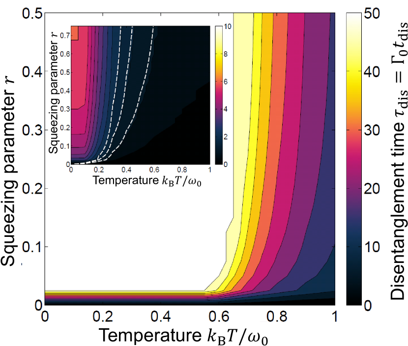
Figure 1: (Color online) Main figure: scaled disentanglement time $\tau_{\rm dis}=\Gamma_{0}t_{\rm dis}$ (colorbar) of nonlinearly damped two-mode squeezed vacuum states as function of temperature $T$ and squeezing parameter $r$, for two individual baths with simulation time $\tau_{\rm sim}=50$, damping rate $\Gamma_{0}=10^{-3}\omega_{0}$, and negativity cut-off $\varepsilon=10^{-3}$. Inset: disentanglement time $\tau_{\rm dis}$ (inset colorbar scale) of linearly damped two-mode squeezed vacuum states as function of $T$ and $r$ for two individual baths, with simulation parameters as in the main figure. The dashed lines are the contours of $\tau_{\rm dis}=\big{[}1,\frac{3}{2},2\big{]}$ (right to left), as theoretically predicted in Prauzner-Bechcicki (2004).

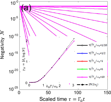
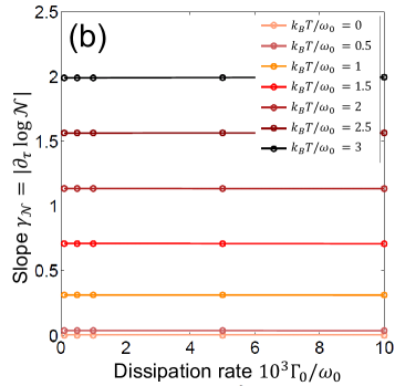
Figure 2: (a) Main figure: Time evolution of the negativity of a nonlinearly damped squeezed two-mode vacuum with squeezing parameter $r=1/20$, individual bath configuration, for temperatures $0\leq k_{\rm B}T/\omega_{0}\leq 3$ and damping rates $\Gamma_{0}=10^{-3}\omega_{0}[1/10,1/2,1,5,10]$. The graphs for the same $T$ and different $\Gamma_{0}$ overlap when plotted as function of $\tau=\Gamma_{0}t$. Inset: Slope of the negativity, $\gamma_{\mathcal{N}}=|\partial_{\tau}\log{\cal N}|$, extracted from the second half of the points in the main figure, as function of $T$ for $\Gamma_{0}=10^{-3}\omega_{0}[1/10,1/2,1,5,10]$ (color code). The dashed line is a slope fit of $2N(2\omega_{0})$. (b) Slope of the negativity $\gamma_{\mathcal{N}}=|\partial_{\tau}\log{\cal N}|$ from the inset in (a) as function of $10^{3}\Gamma_{0}/\omega_{0}$.

III.1 Asymptotic entanglement for coupling to individual baths

For the individual bath configuration and a Markovian model in the RWA, it was shown in Ref. Prauzner-Bechcicki (2004) that for finite temperatures ($T>0$) all linearly damped two-mode squeezed vacuum states disentangle within a finite time, and relax to the ground state. At $T=0$ the relaxation to the ground state occurs in the limit of infinite time. These results were further probed with non-Markovian models in Refs. Maniscalco et al. (2007); Liu and Goan (2007), lending support to the predictions of Ref. Prauzner-Bechcicki (2004). Thus, concluding that the Markovian and non-Markovian dynamics coincide for times larger than reservoir correlation times.

For NLD, earlier studies of a single oscillator systems undergoing NLD show that parity conservation brings the system to a final non-classical steady state Simaan and Loudon (1978); Voje et al. (2013a). For a bipartite system with no inter-mode coupling, it follows that the same parity conservation will, at $T=0$, bring the system into a general steady state

$$\rho(\infty) = P_{00}|00\rangle\langle 00|+P_{11}|11\rangle\langle 11|+\rho_{01,10}|01\rangle\langle 10|$$ (13)

$$+\rho_{10,10}|10\rangle\langle 10|+\Big{[}\rho_{00,11}|00\rangle\langle 11|+$$

$$\rho_{00,01}|00\rangle\langle 01|+\rho_{00,10}|00\rangle\langle 10|+\rho_{01,10}|01\rangle\langle 10|$$

$$+\rho_{01,11}|01\rangle\langle 11|+\rho_{10,11}|10\rangle\langle 11|+\rm{H.c.}\Big{]},$$

with matrix elements $\rho_{ni,mj}$ determined by the initial state. The particular initial state (12) leads to a steady state of the form (13) where several elements are zero, reducing it to

$$\rho(\infty)=P_{00}|00\rangle\langle 00|+P_{11}|11\rangle\langle 11|\\ +(\rho_{00,11}|00\rangle\langle 11|+\rm{H.c})\;.$$ (14)

The element $\rho_{00,11}$ is important for the asymptotic negativity (entanglement). While initially there are multiple off-diagonal elements contributing to the negativity $\mathcal{N}(t=0)=(e^{2|r|}-1)/2$ Paz and Roncaglia (2008), these quickly decohere, leaving only the parity protected matrix elements in (14), and the negativity saturates at $\mathcal{N}(\infty)=|\rho_{00,11}(\infty)|_{T=0}$. This can be verified through the characteristic equation for $\rho^{{\rm T}_{1}}$ of the steady state (14). For a general $M\times M$ basis size the characteristic equation is given by

$$(-\mu)^{M-4}(P_{00}-\mu)(P_{11}-\mu)(\mu^{2}-|\rho_{00,11}|^{2})=0,$$ (15)

with only one negative root $\mu=-|\rho_{00,11}|$.

Comparing the nonlinear and linear decays of squeezed states at $T=0$ one finds that the nonlinearly damped states remain entangled with a saturating negativity, whereas the linearly damped states asymptotically disentangle in the limit of $t\rightarrow\infty$. This can be seen in Fig. 1 showing the scaled disentanglement time $\tau_{\rm dis}$ (colorbar) of a nonlinearly damped (main figure) and linearly damped (inset) two-mode squeezed vacuum as function of $T$ and $r$. The results are obtained from numerical simulations. The scaled disentanglement time is defined as $\tau_{\rm dis}=\Gamma_{0}t_{\rm{dis}}$, where $t_{{\rm dis}}$ is the time at which $\mathcal{N}<\varepsilon$, and $\varepsilon$ is the negativity cut-off. Temperature is measured in units of $\hbar\omega_{0}/k_{\rm B}$. The main figure and inset have identical simulation parameters, but different disentanglement time scales (main and inset colorbars). The white, dashed lines in the inset are the theoretically predicted disentanglement times derived in Ref. Prauzner-Bechcicki (2004).

The nonlinearly and the linearly damped systems for $T>0$ both display a finite disentanglement time for all $r$. The main difference is the disentanglement time scale. The nonlinearly damped states disentangle much slower than the linearly damped states. During the chosen evolution time all LD states disentangle, while a part of the NLD states remain entangled (white region, main figure). After a longer time evolution all NLD states will eventually disentangle.

The time evolution of the negativity while relaxing to the steady state is shown in Fig. 2 (a). Here we use a constant value of $r=1/20$ for several values of $T$ and $\Gamma_{0}$. The graphs for the same $T$ and different $\Gamma_{0}$ overlap when expressed in terms of scaled time units $\tau=\Gamma_{0}t$. Initially the negativity has a rapid initial transient during which the initial squeezed state reduces to a state of the form given by Eq. (14). This is followed by a slow exponential decay.

To quantify the asymptotic decay, the inset in Fig. 2(a) shows the negativity slope $\gamma_{\mathcal{N}}=|\partial_{\tau}\log{\cal N}|$, extracted from the second half of the data in the main panel of Fig. 2(a), as function of $T$. The decay rate solely depends on $T$, which is further corroborated in Fig. 2 (b), showing the negativity slope $\gamma_{\mathcal{N}}$ from (a) as function of $10^{3}\Gamma_{0}$. As shown in appendix A, in the limit of low temperatures, within the RWA, the slope is given by the expression $\mathcal{N}(\tau)=(|\rho_{00,11}(\infty)|_{T=0})e^{-2N(2\omega_{0})\tau}$, shown as the dashed line in the inset to Fig. 2(a).

The much slower decay of the negativity in the nonlinearly damped case compared with the linearly damped system can be understood as follows: For finite temperatures the disentanglement of the nonlinearly damped squeezed vacuum states is related to the slow, thermal dephasing of the parity protected matrix element $\rho_{00,11}$. However, thermal decoherence of this element requires a simultaneous two-quanta excitation of both oscillators, a process which is less probable compared to linear decoherence, where neither an individual nor simultaneous excitation is needed to achieve a de-excitation.

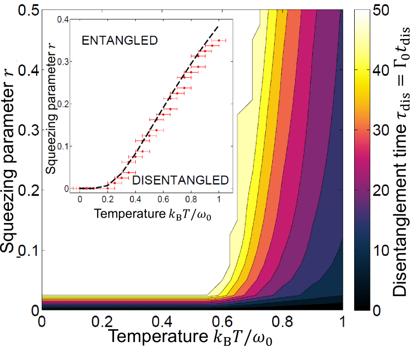
Figure 3: Main figure: disentanglement time $\tau_{\rm dis}=\Gamma_{0}t_{\rm dis}$ (colorbar) of nonlinearly damped two-mode squeezed vacuum states as function of temperature $T$ and squeezing parameter $r$, common bath, with simulation time $\tau_{\rm sim}=50$, damping rate $\Gamma_{0}=10^{-3}\omega_{0}$, and the negativity cut-off $\varepsilon=10^{-3}$. Inset: Entanglement borderline of the linearly damped two-mode squeezed vacuum states, common bath, in the phase space of $r$ and $T$. The dashed line is the theoretical prediction in Prauzner-Bechcicki (2004) and the dots with errorbars are numerical data. The simulation parameters are: $\tau_{\rm sim}=50$, $\Gamma_{0}=10^{-3}\omega_{0}$ and $\varepsilon=10^{-3}$.

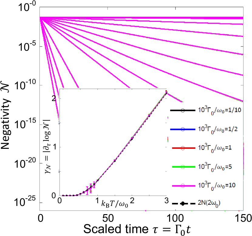
Figure 4: (Color online) Time evolution of the negativity of a nonlinearly damped squeezed two-mode vacuum with squeezing parameter $r=1/20$, common bath configuration, for temperatures $0\leq k_{\rm B}T/\omega_{0}\leq 3$ and damping rates $\Gamma_{0}=10^{-3}\omega_{0}[1/10,1/2,1,5,10]$. The inset shows the slope $\gamma_{\mathcal{N}}$ extracted from the second half of the points in the main figure, as function of $T$ for $\Gamma_{0}=10^{-3}\omega_{0}[1/10,1/2,1,5,10]$ (color code). The dashed line is the function $2N(2\omega_{0})$.

III.2 Asymptotic entanglement for coupling to a common bath

We now turn to the situation with the two independent oscillators nonlinearly coupled to a common reservoir. For a linearly damped system in this configuration, the asymptotic steady states of an initial two mode squeezed state (11) can be divided into entangled and separable states Prauzner-Bechcicki (2004); Paz and Roncaglia (2008, 2009). To which category a state will belong, depends on $r$ and $T$. This result was obtained in Ref. Prauzner-Bechcicki (2004) using Markovian dynamics and RWA and is shown in Fig. 3(inset). An interesting feature is that the system never disentangles for $T=0$. This entanglement preservation can be explained in terms of normal modes, e.g. center of mass and relative coordinates. As only the center of mass motion is affected by the dissipation to the bath, the relative motion of the oscillators evolves freely. For nonlinear system reservoir coupling, there is no decoupling of the relative oscillator motion from the bath, and we do not find any finite temperature steady state entanglement.

As seen in the main figure 3, showing the scaled disentanglement time (colorbar) of nonlinearly damped two-mode squeezed vacuum states as function of $T$ and $r$ for the common bath configuration, the asymptotic entanglement behavior is very similar to the nonlinearly damped squeezed states in the individual bath configuration. Again, the nonlinearly damped states disentangle slower than the linearly damped states in the disentangled region in the inset of Fig. 3. Like in the main panel of Fig. 1, not all states have yet disentangled for the chosen simulation time (white region), but will do so after a longer evolution.

The similarity in the behaviors stem from a supression of information exhange between the oscillators via the bath in the steady state $\rho(\infty)$ for $T\approx 0$. In the QME (9) the term $\mathcal{L}_{1}\rho$ quickly brings the initial state (11) to the steady state (14), which cannot be further affected by the term $\mathcal{L}_{2}\rho$, as $\mathcal{L}_{2}\rho(\infty)=0$. For higher temperatures, the term $\mathcal{L}_{2}\rho$ will contribute to some information exchange, but not enough to significantly alter the influence of the $\mathcal{L}_{1}\rho$-term. The qualitative evolution of the state is therefore as for the individual bath configuration. This is supported by the results in Fig. 4, displaying the slow temperature dependent negativity decay for various $T$ and $\Gamma_{0}$ (main figure), and the temperature dependent negativity decay-rates $\gamma_{\cal N}=|\partial_{\tau}\log{\cal N}|=2N(2\omega_{0})$ (inset). The derivation of the exponent can be found in appendix A and is equal to the thermal decay exponent obtained for individual baths.

IV Results for coupled oscillators

Finally, we consider two weakly coupled oscillators. Based on the results of the preceding section, the main qualitative difference between LD and NLD stems from the parity conservation for the individual oscillators. When the oscillators are coupled only the parity of the entire system is conserved. In particular, the element $\rho_{00,11}$ which we found to give the asymptotic negativity, is no longer protected and can decay via an intermediate transition to the state $\rho_{00,20}$.

Since the situation is close to the linear case, we restrict the discussion to individual baths. The system Hamiltonian (1a) is adjusted to include an inter-mode coupling term

$$H_{\rm S}=\sum_{j=1,2}\left(\frac{1}{2}p_{j}^{2}+\frac{1}{2}\omega_{j}^{2}q_{j}^{2}\right)+\sqrt{\omega_{1}\omega_{2}}\lambda q_{1}q_{2}\;.$$ (16)

The corresponding Hamiltonian in the RWA is

$$H_{\rm S,RWA}=\sum_{j=1,2}\omega_{j}a^{{\dagger}}_{j}a_{j}+\frac{\lambda}{2}a^{{\dagger}}_{j}a_{j-(-1)^{j}}\;.$$ (17)

By the same procedure as described in Sec. II, the RWA-QME for a symmetric system, $\omega_{j}=\omega_{0}$, in the weak intermode coupling limit, $\lambda\ll\omega_{0}$, obtains the form Voje et al. (2013b)

$$\dot{\rho} = -\frac{1}{2}\sum_{j=1,2}\Big{[}\gamma_{j}(2\omega_{0})\mathcal{L}_{1}[a_{j}^{{\dagger}2}]+$$

$$\gamma_{j}(-2\omega_{0})\mathcal{L}_{1}[a_{j}^{2}]\Big{]}\rho+\mathcal{D}_{12}(\lambda)\rho\;.$$

To the lowest order in $\lambda$ the oscillators are individually coupled to their respective reservoirs, and the superoperator $\mathcal{D}_{12}(\lambda)$ becomes

$$\mathcal{D}_{12}(\lambda)\rho={} \Upsilon_{+}\mathcal{L}_{1}[(n_{1}-n_{2})]\rho$$

$$-\frac{1}{2}\Upsilon_{-}\Big{[}(n_{1}-n_{2})(a^{\dagger}_{1}a_{2}-a^{\dagger}_{2}a_{1})\rho\Big{.}$$

$$-(a^{\dagger}_{1}a_{2}-a^{\dagger}_{2}a_{1})\rho(n_{1}-n_{2})$$

$$+\rho(a^{\dagger}_{1}a_{2}-a^{\dagger}_{2}a_{1})^{\dagger}(n_{1}-n_{2})$$

$$\Big{.}-(n_{1}-n_{2})\rho(a^{\dagger}_{1}a_{2}-a^{\dagger}_{2}a_{1})^{\dagger}\Big{]}\;.$$ (19)

Here $\Upsilon_{\pm}=\gamma(\lambda)\pm\gamma(-\lambda)$ with $\gamma(\lambda)=\kappa(\lambda)[N(\lambda)+1]$ and $\gamma(-\lambda)=\kappa(\lambda)N(\lambda)$.

The coupling $\lambda$ plays a dual role of contributing to oscillator interaction via $H_{\rm S}$ and to decoherence via $\mathcal{D}_{12}$. For linearly damped oscillators the decoherence terms in $\mathcal{D}_{12}$ would only arise if $\Gamma_{1}\neq\Gamma_{2}$ de Ponte et al. (2005). There is no such restriction however for the nonlinearly damped system where the superoperator $\mathcal{D}_{12}$ consists of two decoherence terms, proportional to $\Upsilon_{+}$ and $\Upsilon_{-}$ respectively. The temperature dependencies of these terms differ from those of $\gamma_{j}$. For temperatures exceeding the coupling energy, $\lambda\ll k_{\rm B}T$, we have $\Upsilon_{+}>\Upsilon_{-}$. In the low temperature limit, $\lambda\gg k_{\rm B}T$, both terms approach equal magnitudes $\Upsilon_{+}\approx\Upsilon_{-}$.

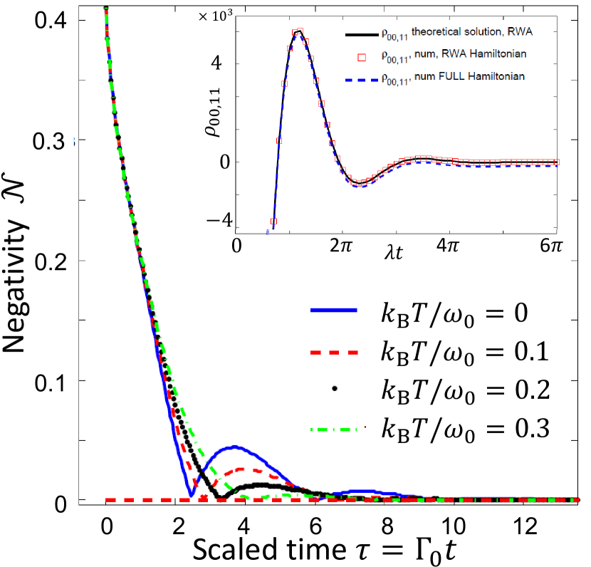
Figure 5: Decay of the negativity $\cal N$ as function of scaled time $\tau=\Gamma_{0}t$ for an initial state with squeezing parameter $r=0.3$ for different temperatures and $\lambda=\Gamma_{0}=10^{-3}\omega_{0}$. The coupling is reflected in the coherent oscillations superposed on the exponential decay towards the thermal equilibrium state. The inset shows the time evolution of $\rho_{00,11}$ of a nonlinearly damped squeezed two-mode vacuum with squeezing parameter $r=1/20$, individual bath configuration, for $T=0$ and damping rate $\lambda=\Gamma_{0}=10^{-3}\omega_{0}$.

For weakly coupled oscillators, linearly coupled to individual baths, a phase diagram separating the entangled steady states from non-entangled steady states exists (see for instance Ref. Galve et al. (2010)). Whether or not the state remains entangled depends on temperature and strength of coupling. A more in depth study, using both Markovian as well as non-Markovian evolution can be found in Ref. Liu and Goan (2007). As explained in Ref. Liu and Goan (2007), starting from an initial two-mode squeezed state, an undamped coupled oscillator system will display coherent oscillations during its time evolution with corresponding oscillations in negativity. Adding finite linear damping, results in loss of entanglement in the long time limit and suppression of coherent oscillations in the negativity.

For the case of nonlinear coupling to individual baths we find results which are similar to those in Ref. Liu and Goan (2007), with coherent oscillations reflected in the decay curve shown in Fig. 5. As can be seen, with increasing temperature the oscillations vanish but the initial rapid decay remains unaltered. The coherent oscillations can be traced back to the time evolution for $T=0$ and $\lambda>0$. In this case, after the transient rapid decay, the negativity dynamics is governed by the evolution of the $\rho_{00,11}$ matrix element. Since the two-mode squeezed vacuum only has even entries, it suffices to analyze the matrix elements with total amount of two quanta. The evolution of $\rho_{00,11}$ is influenced by the elements $\rho_{00,02}$ and $\rho_{00,20}$ which in the RWA approximation contribute to decoherence and hence the asymptotic negativity decays to zero. The detailed calculation is given in Appendix A.3. The resulting time evolution of $\rho_{00,11}$ is shown in the inset of Fig. 5.

Numerically solving the full QME at $T=0$, we see a residual nonzero negativity. This is due to the RWA-Hamiltonian ($H_{\rm S}\propto H_{0}+\lambda(a^{{\dagger}}_{1}a_{2}+a^{{\dagger}}_{2}a_{1})$) not properly reproducing the correct ground state of the coupled oscillator system since terms proportional to $a^{2}$ ($a^{\dagger}a^{\dagger}$) are neglected. Hence, the numerical results display a small residual entanglement. In the inset of Fig. 5 the comparison of the results of the numerical simulation and the RWA shows a very good agreement.

V Conclusions

We have studied the asymptotic behavior of entanglement between two harmonic oscillators when they are quadratically coupled to an environment. In particular, we have investigated to what extent phenomena, known from studying the decay of two-mode squeezed states in the corresponding linearly damped systems, change when damping is nonlinear. We find that the number parity conservation associated with pure nonlinear damping causes significant reduction of the disentanglement rate. Moreover, the equilibrium distribution is different from the standard Bose-distribution. Further, in contrast to the linearly damped systems, we find no qualitative difference between oscillators coupled to common baths and coupled to individual baths. We attribute the latter effect to the lack of a conserved quantity (relative oscillator energy) in the nonlinearly coupled system in compination with a suppressed information exhange between the oscillators at low temperatures. For weakly coupled oscillators, the number parity is no longer individually conserved, hence, the system can relax to the ground state.

The results here are obtained in the Markovian limit. Extending the study to a non-Markovian dynamics could alter the picture presented here. For instance, it is known that for linearly damped oscillator systems studied with non-Markovian dissipation models Liu and Goan (2007); Paz and Roncaglia (2008, 2009), a more detailed and complex picture of the asymptotic behavior emerges. Still, in those studies the overall characteristics obtained in the Markovian limit, for instance the division into entangled and separable steady states, remain intact.

At present it is not known whether it is possible to realize a system where the dominant dissipation mechanism at low excitation levels is purely nonlinear. However, for some dissipation mechanisms, see for instance Ref. Croy et al. (2012), symmetry can dictate that the lowest order coupling to the environment must be quadratic in the coordinates. Systems with such symmetries are thus strong candidates for studying NLD in the quantum regime. Moreover, it was suggested that engineering of NLD might be feasible Nunnenkamp et al. (2010); Leoński and Miranowicz (2004); Everitt et al. (2014). Exploiting the reduced disentanglement in systems with NLD is a promising path towards realizing entanglement based technologies.

Appendix A

A.1 Negativity exponent - individual baths.

Here it is shown that $\gamma_{\cal N}=2N(2\omega_{0})$. As argued in Sec. III.1, $\mathcal{N}(\tau)$ of a nonlinearly damped squeezed state asymptotically only depends on the density matrix element $\rho_{00,11}$. Equation (9) is used to obtain the respective equation of motion, along with equations of motion for elements $X=\sqrt{3}(\rho_{02,13}+\rho_{20,31})$, which influence $\rho_{00,11}$. By assuming that the other elements have already decayed, one obtains a set of two coupled, first order differential equations

$$\dot{\rho}_{00,11} =2\gamma_{2-}X-8\gamma_{2+}\rho_{00,11},$$ (20a)

$$\dot{X} =12\gamma_{2+}\rho_{00,11}-4aX,$$ (20b)

where $a=(\gamma_{2-}+5\gamma_{2+})$ and $\gamma_{2\pm}$ is scaled by $\Gamma_{0}$. For solutions of the form of $\rho_{00,11}\sim Ae^{r_{1}\tau}+Be^{r_{2}\tau}$ on finds,

$$r_{1,2}=-(16\gamma_{2+}+2)\pm 2[(8\gamma_{2+}+1)^{2}-2\gamma_{2+}(21\gamma_{2+}+1)]^{\frac{1}{2}}\;,$$ (21)

where $\gamma_{2-}=\gamma_{2+}+1$ was used. For low $T$, $\gamma_{2+}=N(2\omega_{0})<1$, the square root in (21) can be Taylor expanded up to second order to yield

$$r_{1}\approx-2N(2\omega_{0}),\>\>r_{2}\approx-2(15N(2\omega_{0})+2),$$ (22)

and

$$\rho_{00,11}(\tau)=Ae^{-2N(2\omega_{0})\tau}+Be^{-2(15N(2\omega_{0})+2)\tau},$$ (23)

where the first term denotes the slow thermal decay. The second term describes a rapid initial decay of the matrix element. The amplitudes are given by

$$A =\frac{\rho_{00,11}(0)(11N(2\omega_{0})+2)}{14N(2\omega_{0})+2},$$ (24a)

$$B =\rho_{00,11}(0)\Big{[}1-\frac{11N(2\omega_{0})+2}{14N(2\omega_{0})+2}\Big{]},$$ (24b)

where $\rho_{00,11}(0)$ is given by (12). Also, $A>0$ for all $r>0$ and $A\gg B$ for low $T$. Hence $\gamma_{\cal N}=2N(2\omega_{0})\tau$.

A.2 Negativity exponent - common bath.

Here we verify that the decay of entanglement, as governed by the matrix element $\rho_{00,11}$, for the individual bath case is $\gamma_{\cal N}=2N(2\omega_{0})$. With the same assumptions as for the individual baths, from equation (9) one obtains the equations of motion for the matrix elements responsible for the negativity in the common bath case

$$\dot{\rho}_{00,11} =2\sqrt{3}\gamma_{2-}Z-8\gamma_{2+}\rho_{00,11},$$ (25a)

$$\dot{Z} =8\sqrt{3}\gamma_{2+}\rho_{00,11}-8(\gamma_{2-}+3\gamma_{2+})Z,$$ (25b)

where $Z=\rho_{02,13}+\rho_{02,31}+\rho_{20,13}+\rho_{20,31}$. In this case we obtain the solution

$$\rho_{00,11}=Ce^{-2N(2\omega_{0})\tau}+De^{-2(19N(2\omega_{0})+4)\tau},$$ (26)

with the amplitudes

$$C =\frac{\rho_{00,11}(0)(15N(2\omega_{0})+4)}{18N(2\omega_{0})+4}$$ (27a)

$$D =\rho_{00,11}(0)\Big{[}1-\frac{15N(2\omega_{0})+4}{18N(2\omega_{0})+4}\Big{]},$$ (27b)

where $\rho_{00,11}(\tau=0)$ is given in (12). Also, $C>0$ for all $r>0$ and $C\gg D$ for low $T$. Hence the decay rate is again dominated by $\gamma_{\cal N}=2N(2\omega_{0})$.

A.3 Negativity evolution - individual bath, non-zero inter-mode coupling.

For $T=0$ and an inter-mode coupling $\lambda>0$ the evolution of negativity is still governed by the $\rho_{00,11}$ element. For an initially two-mode squeezed state, the equations of motion governing the evolution are

$$\dot{\rho}_{00,11} =\frac{\rm{i}\lambda}{\sqrt{2}}Y\;,$$ (28a)

$$\dot{Y} =(\rm{i}\sqrt{2}\lambda-2\sqrt{2}\Upsilon)\rho_{00,11}-(\gamma_{2-}+2\Upsilon)Y,$$ (28b)

where $Y=\rho_{00,02}+\rho_{00,20}$. For a solution of the form $\rho_{00,11}=A_{+}e^{r_{+}\tau}+A_{-}e^{r_{-}\tau}$ one finds

$$r_{\pm}=-\frac{1}{2}(\Gamma_{0}+2\Upsilon)\pm\frac{1}{2}\sqrt{(\Gamma_{0}+2\Upsilon)^{2}-4(\lambda^{2}+\rm{i}2\lambda\Upsilon)},$$ (29)

with amplitudes

$$A_{+} =-\frac{\rho_{00,11}(0)r_{-}}{(r_{+}-r_{-})}\;,$$ (30a)

$$A_{-} =\rho_{00,11}(0)\Big{[}1+\frac{r_{-}}{(r_{+}-r_{-})}\Big{]}\;.$$ (30b)

References

- Einstein et al. (1935) A. Einstein, B. Podolsky, and N. Rosen, Phys. Rev. 47, 777 (1935).
- Schrödinger (1935) E. Schrödinger, Naturwiss. 23, 807 (1935).
- Horodecki et al. (2009) R. Horodecki, P. Horodecki, M. Horodecki, and K. Horodecki, Rev. Mod. Phys. 81, 865 (2009).
- Ekert (1991) A. K. Ekert, Phys. Rev. Lett. 67, 661 (1991).
- Bennett and Wiesner (1992) C. H. Bennett and S. J. Wiesner, Phys. Rev. Lett. 69, 2881 (1992).
- Shor (1995) P. W. Shor, Phys. Rev. A 52, R2493 (1995).
- Yurke and Stoler (1992) B. Yurke and D. Stoler, Phys. Rev. A 46, 2229 (1992).
- Bennett et al. (1993) C. H. Bennett, G. Brassard, C. Crépeau, R. Jozsa, A. Peres, and W. K. Wootters, Phys. Rev. Lett. 70, 1895 (1993).
- Bose et al. (1998) S. Bose, V. Vedral, and P. L. Knight, Phys. Rev. A 57, 822 (1998).
- Bouwmeester et al. (1997) D. Bouwmeester, J.-W. Pan, K. Mattle, M. Eibl, H. Weinfurter, and A. Zeilinger, Nature 390, 575 (1997).
- Boschi et al. (1998) D. Boschi, S. Branca, F. De Martini, L. Hardy, and S. Popescu, Phys. Rev. Lett. 80, 1121 (1998).
- Furusawa et al. (1998) A. Furusawa, J. L. Sørensen, S. L. Braunstein, C. A. Fuchs, H. J. Kimble, and E. S. Polzik, Science 282, 706 (1998).
- Pfaff et al. (2014) W. Pfaff, B. J. Hensen, H. Bernien, S. B. van Dam, M. S. Blok, T. H. Taminiau, M. J. Tiggelman, R. N. Schouten, M. Markham, D. J. Twitchen, et al., Science 345, 532 (2014).
- Prauzner-Bechcicki (2004) J. S. Prauzner-Bechcicki, Journal of Physics A: Mathematical and General 37, L173 (2004).
- Benatti and Floreanini (2006) F. Benatti and R. Floreanini, Journal of Physics A: Mathematical and General 39, 2689 (2006).
- Maniscalco et al. (2007) S. Maniscalco, S. Olivares, and M. G. A. Paris, Phys. Rev. A 75, 062119 (2007).
- Liu and Goan (2007) K.-L. Liu and H.-S. Goan, Phys. Rev. A 76, 022312 (2007).
- Paz and Roncaglia (2008) J. P. Paz and A. J. Roncaglia, Phys. Rev. Lett. 100, 220401 (2008).
- Paz and Roncaglia (2009) J. P. Paz and A. J. Roncaglia, Phys. Rev. A 79, 032102 (2009).
- Galve et al. (2010) F. Galve, L. A. Pachón, and D. Zueco, Phys. Rev. Lett. 105, 180501 (2010).
- Yu and Eberly (2004) T. Yu and J. H. Eberly, Phys. Rev. Lett. 93, 140404 (2004).
- Serafini et al. (2004) A. Serafini, F. Illuminati, M. G. A. Paris, and S. De Siena, Phys. Rev. A 69, 022318 (2004).
- Simaan and Loudon (1978) H. D. Simaan and R. Loudon, J. Phys. A 11, 435 (1978).
- Kronwald et al. (2013) A. Kronwald, F. Marquardt, and A. A. Clerk, Phys. Rev. A 88, 063833 (2013).
- Voje et al. (2013a) A. Voje, A. Croy, and A. Isacsson, New Journal of Physics 15, 053041 (2013a).
- Dykman and Krivoglaz (1984) M. Dykman and M. Krivoglaz, Soviet Scientific Reviews, Section A, Physics Reviews 5, 265 (1984).
- Eichler et al. (2011) A. Eichler, J. Moser, J. Chaste, M. Zdrojek, I. Wilson-Rae, and A. Bachtold, Nat. Nanotechnol. 6, 339 (2011).
- Croy et al. (2012) A. Croy, D. Midtvedt, A. Isacsson, and J. M. Kinaret, Phys. Rev. B 86, 235435 (2012).
- Nunnenkamp et al. (2010) A. Nunnenkamp, K. Børkje, J. G. E. Harris, and S. M. Girvin, Phys. Rev. A 82, 021806 (2010).
- Leoński and Miranowicz (2004) W. Leoński and A. Miranowicz, J. Opt. B 6, S37 (2004).
- Everitt et al. (2014) M. J. Everitt, T. P. Spiller, G. J. Milburn, R. D. Wilson, and A. M. Zagoskin, Quantum Computing 1, 1 (2014).
- Voje et al. (2013b) A. Voje, A. Isacsson, and A. Croy, Phys. Rev. A 88, 022309 (2013b).
- Simon (2000) R. Simon, Phys. Rev. Lett. 84, 2726 (2000).
- Braunstein and van Loock (2005) S. L. Braunstein and P. van Loock, Rev. Mod. Phys. 77, 513 (2005).
- Breuer and Petruccione (2002) H. P. Breuer and F. Petruccione, The Theory of Open Quantum Systems (Oxford University Press, USA, 2002).
- Wangsness and Bloch (1953) R. K. Wangsness and F. Bloch, Phys. Rev. 89, 728 (1953).
- Bloch (1957) F. Bloch, Phys. Rev. 105, 1206 (1957).
- Redfield (1965) A. G. Redfield, Adv. Magn. Reson. 1, 1 (1965).
- Drummond and Ficek (2004) P. Drummond and Z. Ficek, Quantum Squeezing, Physics and Astronomy Online Library (Springer, 2004), ISBN 9783540659891.
- Vidal and Werner (2002) G. Vidal and R. F. Werner, Phys. Rev. A 65, 032314 (2002).
- de Ponte et al. (2005) M. de Ponte, M. de Oliveira, and M. Moussa, Ann. Phys. 317, 72 (2005).